An Evaluation of Spring Flows to Support theUpper San Marcos River Spring Ecosystem, Hays County, Texas

Kenneth S. SaundersKevin B. Mayes

Tim A. Jurgensen

Joseph F. TrungaleLeroy J. Kleinsasser

Karim Aziz

Jacqueline Renée FieldsRandall E. Moss

River Studies Report No. 16

Resource Protection Division

Texas Parks and Wildlife DepartmentAustin, Texas

August 2001

i

Table of Contents

An Evaluation of Spring Flows to Support the Upper San Marcos River Spring Ecosystem,Hays County, Texas

Introduction..........................................................................................................................................1

Methods ................................................................................................................................................6

Results ................................................................................................................................................12

Segment Description........................................................................................................................12Mesohabitat Description....................................................................................................................13Hydraulic Models ..............................................................................................................................15Macrophyte Data Summaries .............................................................................................................15Fish Data Summary ...........................................................................................................................16Suitability Criteria ..............................................................................................................................16Instream Habitat Model......................................................................................................................17Habitat Time Series...........................................................................................................................18Critical Depths for Z. texana ...............................................................................................................20Water Quality....................................................................................................................................20

Discussion ..........................................................................................................................................23

Historical Hydrology ..........................................................................................................................24Rich Biodiversity...............................................................................................................................24Dominance of Run-type Mesohabitats................................................................................................25Water Quality....................................................................................................................................25Recreation .......................................................................................................................................28Spring Flow and Ecosystem Characteristics........................................................................................28

Acknowledgments.............................................................................................................................30

References.........................................................................................................................................30

ii

List of Figures

FIGURE 1.—Daily mean flow based on spring flows recorded at USGS Gage #08170000 (San MarcosSprings at San Marcos, TX) for the period of record 26 May 1956–30 September 1998. Monthlyaverage naturalized flows were developed for the period from January 1934–December 1989 (HDREngineering, Inc. 1993). Daily median equal to 157 ft3/s based on USGS record. ....................................3

FIGURE 2.—Flow frequencies are based on daily spring flows recorded at USGS Gage #08170000 (SanMarcos Springs at San Marcos, TX) for the period of record 26 May 1956–30 September 1998. Barsrepresent frequency in bins (5 ft3/s) and solid line represents cumulative frequency percentage.There are 15,468 daily records for this period. ......................................................................................3

FIGURE 3.—Watershed of the upper San Marcos River................................................................................4

FIGURE 4.—Study area of the upper San Marcos River. ...............................................................................7

FIGURE 5.—Bio-grid sampling sites used for habitat availability and utilization data collection on the upperSan Marcos River. ...............................................................................................................................9

FIGURE 6.—Normalized wetted width in pool, riffle, and run mesohabitats in relation to discharge in theupper San Marcos River. Data based on all modeled cross-sections in the main channel (upper) and inthe natural channel (lower). Main channel wetted width normalized to long-term median spring flow(1956-1998). Natural channel wetted width normalized to 140 ft3/s.......................................................15

FIGURE 7.—Zizania texana percent weighted usable area (% WUA) in relation to spring flow in the upperSan Marcos River main channel segments..........................................................................................18

FIGURE 8.—Heteranthera liebmannii percent weighted usable area (% WUA) in relation to spring flow inthe upper San Marcos River main channel segments...........................................................................18

FIGURE 9.—Vallisneria americana percent weighted usable area (%WUA) in relation to spring flow in theupper San Marcos River main channel segments. ...............................................................................18

FIGURE 10.—Sagittaria platyphylla percent weighted usable area (% WUA) in relation to spring flow in theupper San Marcos River main channel segments. ...............................................................................18

FIGURE 11.—Potamogeton illinoensis percent weighted usable area (%WUA) in relation to spring flow inthe upper San Marcos River main channel segments...........................................................................18

FIGURE 12.—Spring flow ranges that contribute to above average habitat conditions based on 75thpercentile %WUA frequencies calculated from habitat time series. Vertical lines represent 25th and75th percentile spring flows...............................................................................................................19

FIGURE 13.—Spring flow ranges that contribute to average habitat conditions based on 25th-75thpercentile %WUA frequencies calculated from habitat time series. Vertical lines represent 25th and75th percentile spring flows...............................................................................................................19

FIGURE 14.—Spring flow ranges that contribute to below average habitat conditions based on 25thpercentile %WUA frequencies calculated from habitat time series. Vertical lines represent 25th and75th percentile spring flows...............................................................................................................19

FIGURE 15.—San Marcos River, temperature by station, measured hourly, Nov-1994 through May-1997.Horizontal line in box: sample median. Box top and bottom: 75th and 25th percentiles. Upper andlower fences: limits of data.................................................................................................................21

FIGURE 16.—San Marcos River, summer conditions, temperature by station, measured hourly, May-1996through Jul-1996. Horizontal line in box: sample median. Box top and bottom: 75th and 25thpercentiles. Upper and lower fences: limits of data. .............................................................................21

FIGURE 17.—San Marcos River, winter conditions, temperature by station, measured hourly, Dec-1995through Feb-1996. Horizontal line in box: sample median. Box top and bottom: 75th and 25thpercentiles. Upper and lower fences: limits of data. .............................................................................21

iii

FIGURE 18.—San Marcos River, dissolved oxygen (mg/L) by station, measured hourly, Nov-1994 throughMay-1997. Horizontal line in box: sample median. Box top and bottom: 75th and 25th percentiles.Upper and lower fences: limits of data.................................................................................................22

FIGURE 19.—San Marcos River, summer conditions, dissolved oxygen by station, measured hourly, May-1996 through Jul-1996. Horizontal line in box: sample median. Box top and bottom: 75th and 25thpercentiles. Upper and lower fences: limits of data. .............................................................................22

FIGURE 20.—San Marcos River, winter conditions, dissolved oxygen by station, measured hourly, Dec-1995 through Feb-1996. Horizontal line in box: sample median. Box top and bottom: 75th and 25thpercentiles. Upper and lower fences: limits of data. .............................................................................22

FIGURE 21.—San Marcos River, pH by station, measured hourly, Nov-1994 through May-1997. Horizontalline in box: sample median. Box top and bottom: 75th and 25th percentiles. Upper and lower fences:limits of data......................................................................................................................................22

FIGURE 22.—San Marcos River, specific conductance by station, measured hourly, Nov-1994 throughMay-1997. Horizontal line in box: sample median. Box top and bottom: 75th and 25th percentiles.Upper and lower fences: limits of data.................................................................................................23

FIGURE 23.—San Marcos River, turbidity by station, measured twice per month, Nov-1994 through May-1997. Horizontal line in box: sample median. Box top and bottom: 75th and 25th percentiles. Upperand lower fences: limits of data...........................................................................................................23

FIGURE 24.—Flowchart relating San Marcos Springs ecosystem characteristics to spring flow. Peak flowsrefer to runoff events not included in the San Marcos spring flow record (USGS Gage #08170000)........29

iv

List of Tables

TABLE 1.—Daily flow (ft3/s) statistics for USGS Gage #08170000 San Marcos Springs at San Marcos, TX.Based on period of record from May 26, 1956 to September 30, 1998...................................................2

TABLE 2.—Modified Wentworth scale substrate codes................................................................................8

TABLE 3.—Conditions at water quality sampling stations............................................................................11

TABLE 4.—Statistics for temperature, dissolved oxygen, pH, specific conductance and turbidity for SanMarcos River water quality stations 1-7. Deployment periods — Stations 1 and 2: Nov-1994 throughMay-1997; 3 and 4: Feb-1995 through Mar-1997; 5: Nov-1994 through Mar-1997; 6: Mar-1995through Mar-1997; 7: Dec-1995 through May-1997............................................................................20

TABLE 5.—Number of months that threshold temperatures are exceeded as predicted by the SNTEMPmodel for each station (3, 4, and 5). Actual flow and meteorological conditions were used for 1995 and1996. Synthetic data sets include median and minimum flow scenarios assuming normal and 85thpercentile air temperatures.. ..............................................................................................................23

TABLE 6.—San Marcos River water temperature measurements greater than or equal to 25° C.....................26

TABLE 7.—Dissolved oxygen (DO) values failing to meet TNRCC water quality standards. All data based onfirst four days of deployment following calibration. Station 7 met all DO criteria (High aquatic life use) forsegment 1808..................................................................................................................................27

TABLE 8.—Specific conductance results compared to the state surface water quality standard for totaldissolved solids (TDS). Attainment of the TDS standard is based on the mean of at least 4measurements in one year from all stations within the segment............................................................28

An Evaluation of Spring Flows to Support the Upper San Marcos RiverSpring Ecosystem, Hays County, Texas

KENNETH S. SAUNDERS, KEVIN B. MAYES, TIM A. JURGENSEN,JOSEPH F. TRUNGALE, LEROY J. KLEINSASSER, KARIM AZIZ,

JACQUELINE RENÉE FIELDS, AND RANDALL E. MOSS

Resource Protection Division, Texas Parks and Wildlife Department, Austin, Texas

Abstract.—The upper San Marcos River spring ecosystem in central Texas is fed by the EdwardsAquifer and provides habitat for a diverse aquatic community. An instream flow study was undertaken todetermine the water quantity and quality needs of this spring ecosystem. Instream habitat modelingrevealed spatial variation in habitat-spring flow relationships for target aquatic macrophytes. Spring flowsbetween 125 and 200 ft3/s, of sufficient duration, maintain average habitat conditions for all target speciesin all study segments. Empirical water quality data indicated a downstream longitudinal trend of increasingtemperature in warm months and decreasing temperature during cool months. The temperature modelpredicted that violations of temperature criteria could occur during hot summer months. Spring ecosystemcharacteristics which define the upper San Marcos River can only be maintained by a flow regime thatconsists of normal, less than normal, and greater than normal spring flows concordant with historicalduration and frequency, in addition to the full range of peak flows necessary for flushing, scouring,sediment transport, and channel maintenance.

Waters issuing from San Marcos Springs along theBalcones Fault Zone give rise to the San MarcosRiver within the city limits of San Marcos, HaysCounty, Texas. The springs are fed by the EdwardsAquifer which extends approximately 180 miles fromKinney County in the west (2000 ft mean sea level[MSL ft]) eastward to Hays County and the SanMarcos Springs (574 MSL ft). The aquifer isgeohydrologically divided into two segments, thenorthern (Barton Springs) and southern (SanAntonio) segment, which contains the San MarcosSprings (McKinney and Sharp 1995). The aquiferrecharge zone lies along the southern and easternportions of the Edwards Plateau and coversapproximately 1101 mi2 of mostly karst topography(USFWS 1996). San Marcos Springs are the secondlargest in Texas and have historically exhibited themost constant discharge of any spring system in thesouthwestern United States, never having ceasedto flow within recorded history (Brune 1981).

Uninterrupted habitation of the San MarcosSprings area by Native Americans has beendocumented from about 9500 BC (Shiner 1983).Use of the upper San Marcos River as a source ofirrigation water and as a power source to run millsbegan in the mid 1800s (Taylor 1904). Spring LakeDam was constructed in 1849 to run a mill and forirrigation purposes. By 1905 six additional dams,including Rio Vista Dam and Cummings’ Dam, hadbeen constructed for various uses. Other activitiesincluded dredging, channelization, bankstabilization, construction of diversion canals suchas Thompson's millrace and five floodcontrol/recharge structures in the upper San Marcos

watershed (USFWS 1996). Currently, the SanMarcos River and the Springs are importantrecreation attractions within the City of San Marcosand are visited by thousands annually (Bradsby1994).

The San Marcos River provides habitat for adiverse spring flow dependent aquatic community.The foundation of this aquatic ecosystem is thediverse and abundant macrophyte assemblage(Longley 1991). The aquatic community includescommon Edwards Plateau species, variousintroduced species, as well as several endemicswhich lend evidence that the system is truly unique.Spring flow (hereafter referred to as flow)characteristics include high water clarity andrelatively constant flow rates, temperatures, pH, anddissolved ion concentrations (Hannan and Dorris1970; Ogden et al. 1985; TNRCC 1996; Groeger etal. 1997; Slattery and Fahlquist 1997).

Given the historically stable nature of flow fromSan Marcos Springs, vulnerability to negative impactis greater than in other aquatic ecosystemsaccustomed to seasonal changes in water quantityand quality. The Edwards Aquifer remains theprincipal source and in some cases the sole sourceof water for a rapidly growing central Texaspopulation and for large metropolitan areas such asSan Antonio. Primary threats to the ecosysteminclude reduction and cessation of flow due topumping, poor water quality, non-point pollution,habitat modifications, the presence of a multitude ofnon-native species, impacts due to recreationalactivities and urbanization of the river corridor(USFWS 1996).

2

Conservation of the quantity and quality ofEdwards Aquifer water emanating from the springs isfundamental to the preservation of this springecosystem. In addition, stable flows provide baseflows in downstream reaches of the San Marcos andGuadalupe rivers which sustain fish and wildliferesources. When combined, the San MarcosSprings and nearby Comal Springs provideapproximately 32% of Guadalupe River base flow tothe estuarine environments of San Antonio Bay,Texas, and provide 70% or more of base flow duringdroughts (GBRA 1988).

The River Studies Program of the Texas Parks andWildlife Department initiated this instream flow studyof the upper San Marcos River in an effort tounderstand the water quantity and quality needs ofthe spring ecosystem. Study design was directed atyielding estimates of flow as well as water qualityconditions necessary to support and maintain thisunique spring run ecosystem. Objectives were to:(1) determine habitat suitability criteria for targetspecies of the aquatic community; (2) develop aninstream habitat model that simulates changes inphysical habitat in relation to flow; (3) determine howchanges in flow relate to suitable habitat for targetspecies; (4) describe trends in water quality fromempirical and simulated data sets; and (5) describeflow levels that will conserve and promote the fishand wildlife resources of the San Marcos River.

Historical hydrology.–The period of record used todevelop historical hydrology was 26 May 1956 to 30September 1998 based on daily spring flow datacollected at USGS Gage #08170000 (San MarcosRiver Springflow at San Marcos, TX). Early accountsof the San Marcos Springs describe flow asemerging with sufficient force to form a fountainthree feet high and estimates of annual streamflowfor the San Marcos River are available as far back as1892 (Brune 1981); however, records prior to 1916may not be accurate as they were likely corrupted byvarious dams and diversions (Guyton & Associates1979). Other streamflow records collectedintermittently by the USGS or estimated by theTexas Water Development Board (TWDB) prior to1956 have been used to develop a monthly-naturalized streamflow set for the period 1934-1989(HDR Engineering, Inc. 1993). In addition toincorporating pre-USGS gage data the naturalizedflow set includes adjusted flow records fordiversions and returns for the period 1956-1988.While Figure 1 indicates that 1939 and 1952 werevery dry, the drought of record, which occurredduring the summer of 1956, is within the USGSgage flow record.

Monthly median flows (Table 1) exhibit a narrowrange (147 to 182 ft3/s). The long-term mean flow forthe period of record is 167 ft3/s and the long-termmedian is 157 ft3/s. Lowest flows occur in the

summer months as a result of climatological factorsand increased seasonal pumping from the EdwardsAquifer. The lowest flow on record (46 ft3/s)occurred on 15 and 16 August 1956. Highest springflows occur in the spring and the highest spring flowon record (451 ft3/s) occurred on 12 March 1992.Figure 2 shows frequencies of observed flows. Thenarrow range of flows observed in the San MarcosRiver is again highlighted by the fact that about 60%of all observed flows were between 118 and 211ft3/s.

TABLE 1.—Daily flow (ft3/s) statistics for USGS Gage #08170000San Marcos Springs at San Marcos, TX. Based on period of recordfrom May 26, 1956 to September 30, 1998.

Month Mean Min 20a Median 80a Max

Jan 163 68 118 152 200 393Feb 167 65 119 157 200 431Mar 170 82 118 157 212 451Apr 170 89 119 162 215 439May 180 65 127 172 224 421Jun 190 54 122 182 240 427Jul 179 48 107 172 231 403Aug 164 46 114 162 210 353Sep 155 50 116 152 192 289Oct 153 59 118 152 193 310Nov 155 65 118 147 190 316Dec 160 60 118 147 206 385All Months 167 46 118 157 211 451

a - Percentile

Of 281 major springs in the state, 65 springs havedried up, the vast majority during the 20th century(Ono et al. 1983). Spring systems fed by theEdwards Aquifer account for approximately 55% ofthe water leaving the Edwards Aquifer, with theremaining 45% removed via pumping (Brown et al.1992). Pumping from the Edwards Aquifer firstbegan in the late 19th century (Maclay 1989; Ewing2000). Recharge rates have at times fallen belowwithdrawal rates causing the Edwards pool level tolower and some spring orifices (such as San PedroSprings) along the Balcones Escarpment to ceaseflowing. Given mean annual recharge rates of600,000 acre-feet (GBRA 1988) it is feared thatpumping from the Edwards Aquifer might soonexceed average annual recharge. During the 1956drought Comal Springs ceased flowing for nearly 6months and discharge from the San Marcos Springsfell to it's record low. Pumping from the EdwardsAquifer most threatens the San Marcos River springecosystem. Projections given current populationgrowth offer only a 50 to 75 percent chance ofcontinuous flow at San Marcos Springs by the year2020 (USBR 1974).

Peak flows have been altered by five floodwaterretention dams built on two creeks (Purgatory andSink Creeks) which feed the San Marcos River withinthe city limits (Figure 3).

Water quality.–Waters issuing from the SanMarcos Springs are characterized by relativelyconstant temperatures, pH, and dissolved ion

3

FIGURE 1.—Daily mean flow based on spring flows recorded at USGS Gage #08170000 (San MarcosSprings at San Marcos, TX) for the period of record 26 May 1956–30 September 1998. Monthly averagenaturalized flows were developed for the period from January 1934–December 1989 (HDR Engineering, Inc.1993). Daily median equal to 157 ft3/s based on USGS record.

FIGURE 2.—Flow frequencies are based on daily spring flows recorded at USGS Gage #08170000 (SanMarcos Springs at San Marcos, TX) for the period of record 26 May 1956–30 September 1998. Bars representfrequency in bins (5 ft3/s) and solid line represents cumulative frequency percentage. There are 15,468 dailyrecords for this period.

0

50

100

150

200

250

300

350

400

450

500

550

1930 1935 1940 1945 1950 1955 1960 1965 1970 1975 1980 1985 1990 1995 2000

USGS Gage Daily Mean

Monthly Average Naturalized Flow

Drought of Record

Daily Median

Dai

ly m

ean

sprin

g flo

w (

ft /s

)3

0%

10%

20%

30%

40%

50%

60%

70%

80%

90%

100%

45 65 85 105

125

145

165

185

205

225

245

265

285

305

325

345

365

385

405

425

445

Spring flow (ft3/s)

Cum

ulat

ive

freq

uenc

y pe

rcen

tage

0

100

200

300

400

500

600

700

Fre

quen

cyFlow is less than 125 ft3/s 25% of the time

Flow is less than 157 ft3/s 50% of the time

Flow is less than 200 ft3/s 75% of the time

4

FIGURE 3.—Watershed of the upper San Marcos River.

concentrations. Water temperatures at the springsaverage approximately 22°C (Guyton and Associates1979; Ogden et al. 1985). Temperature variabilityincreases with distance from the springs (Groeger etal. 1997). Spring discharge samples collected in1984 and 1985 (Ogden et al. 1985) yielded totalalkalinity values between 200 and 300 mg/L asCaCO3 with pH values primarily between 7 and 8,conditions which favor stable pH levels in the riverdownstream. In the upper San Marcos River, medianpH in summer 1994 ranged from 7.4 to 7.8 (Slatteryand Fahlquist 1997) with higher values noteddownstream. At the spring source carbon dioxide(CO2) levels are typically high while dissolvedoxygen (DO) levels are depressed (Groeger et al.1997). DO levels rise rapidly and approachatmospheric equilibrium downstream of Spring Lakeas a result of vigorous mixing of water at the spillway(Hannan and Dorris 1970). Downstream from SpringLake, DO measurements have generally rangedfrom 7 to 10 mg/L (TNRCC 1996; Groeger et al.1997; Slattery and Fahlquist 1997). Specificconductance at the springs has generally rangedfrom 500 to 600 µS/cm (Ogden et al. 1985; Guytonand Associates 1979). Measurements in the upperriver for the period 1990-1994 ranged from 444 to

599 µS/cm (TNRCC 1996). Median values duringsummer 1994 ranged from 577 to 590 µS/cm(Slattery and Fahlquist 1997). Turbidity levels withinthe upper river are very low, but increasedownstream (Groeger et al. 1997). Clear, thermallyconstant water combined with relatively constantnutrient levels promote an abundant aquaticmacrophyte community in the upper river. Theaquatic macrophyte community exerts significanteffect on DO and CO2 diel variation, and reducesnitrate concentrations (Groeger et al. 1997).

TNRCC designates the upper portion of the SanMarcos River (Segment 1814: extending from apoint 0.6 mile upstream of the confluence with theBlanco River in Hays County to a point 0.4 mileupstream of Loop 82 in San Marcos) as effluentlimited, suitable for contact recreation and to have anexceptional aquatic life use (TNRCC 1995).

Decreased flows are a concern relative to waterquality because parameters like water temperatureand DO could fluctuate more broadly andsignificantly reduce the proportion of springecosystem habitat in the river. Given the historicallystable nature of water quality in the system, spring-adapted species may be adversely affected by wideswings in certain parameters (USFWS 1996). Some

S anM

ar cos

0 2 4 6 8 10 12 14miles

San Marcos

Spring

Lake

Creek

Creek

Springs

N

sub-basin boundary

flood control structure

Produced by: River Studies, Resource Protection, TPWD

UPPER SAN MARCOS RIVER WATERSHED

SanM

arcos

Willow

Sink

Purgatory

5

have speculated that reduced aquifer levels mayresult in decreased water quality from intrusion ofsaline water from the “bad water zone” into thefreshwater zone, which directly feeds the springs(USFWS 1996). Decreased flows also magnifyconcerns about point and non-point sourcepollution, since the assimilative capacity of the riverwould be reduced.

Habitat.–Historic accounts of the headwaters ofthe San Marcos River describe a run-dominatedsystem (Brune 1981; Vaughn 1986). Terrell et al.(1978) described the upper San Marcos River as arapidly flowing clear river, with firm gravel substrateand many shallow areas alternating with pools.Damming of the river and associated diversions formunicipal, industrial and irrigational uses havealtered natural hydraulic conditions resulting in lossof run and riffle habitat and an increase in backwaterand pool habitat, which are characterized by lowcurrent velocity, greater depths and a tendency toaccumulate silt. Altered habitat in the lower reach ofthe upper San Marcos Spring ecosystem is likelydue in part to the presence of Cummings’ Dam,which has a noticeable physico-chemical effect onthe river (Espy, Huston and Associates 1975).Further, the authors stated that flood controlstructures designed to prevent bank-full flows,when coupled with projected decreases in springflow, would have a high probability of damaging theaquatic community. The five flood control/rechargedams in the upper San Marcos watershed (Figure 3)have reduced both the intensity and frequency ofbank-full events (USFWS 1996) and resulted inincreased levels of sedimentation (Wood and Gilmer1996).

Reductions in flow result in reduced habitat areaand altered hydraulic conditions. Long termreductions will result in adjustments in channelmorphometry and consequent redistribution ofmicrohabitats (Espy, Huston and Associates 1975).Introduced species, primarily non-native aquaticmacrophytes have further altered historic habitat(USFWS 1996).

Biology.–Continuous spring flows, exceptionalwater quality, moderate temperatures, and anaverage growing season of 254 days, have overtime allowed the diverse aquatic macrophytecommunity of the San Marcos Springs ecosystem todevelop. The macrophyte community provides bothforage and cover for fish and other aquatic species.Lemke (1989) reported 31 macrophyte species fromthe San Marcos spring ecosystem of which 23 arenative. Potamogeton illinoensis and Sagittariaplatyphylla were described as dominant species. Ofconcern is Texas wild-rice (Zizania texana), whosepopulation has declined over time and is listed byboth state and federal agencies as an endangeredspecies. Z. texana has a very limited habitat range

and exists world-wide only in the upper portions ofthe San Marcos River. It is a large perennial aquaticgrass adapted to shallow, clear, swift-flowing, andconstant temperature water (Emery 1967). At onetime the species was abundant and prolific within theupper 2.5 miles of river (Emery 1967) and was adominant species in the area upstream of SpringLake Dam during the 1930's and 40's (Watkins1930; Devall 1940). Annual surveys of arealcoverage of Z. texana indicate the population isgreatly reduced in size compared to historicdescriptions (Silveus 1933; Devall 1940; Emery1967; Beaty 1975; Emery 1977; Terrell et al. 1978;USFWS 1984; Poole and Bowles 1996). Recentfloods and dam breaches may have further reducedit's abundance (TPWD observations).

A total of 56 fish species, of which 44 are native,have been reported from the upper San MarcosRiver (GFCT 1958; Young et al. 1973; Kelsey 1997).Some such as catfish, bass, crappie, and sunfishsupport sport fishing along the entire San MarcosRiver. Listed as endangered by the USFWS and theState of Texas are the endemic San Marcosgambusia (Gambusia georgei) and the fountaindarter (Etheostoma fonticola). No San Marcosgambusia have been collected since 1982 and thespecies is considered extinct (USFWS 1996).Historically fountain darter were found from thespring source to Ottine but currently its’ distributionis from the spring source downstream to betweenthe City of San Marcos Wastewater Treatment Plant(WWTP) and the Blanco River confluence (USFWS1996). Fountain darters utilize habitats with lowcurrent velocity and dense aquatic vegetation(Schenck and Whiteside 1976; Linam 1993).

The San Marcos salamander (Eurycea nana), SanMarcos saddle-case caddisfly (Protoptila arca) andthe giant river shrimp (Macrobrachium carcinus) areof interest given their distribution, population sizeand susceptibility to anthropogenic impact (USFWS1996; Bowles et al. 2000).

Introduction of exotic species has exertedsignificant effect on the system over time and haschanged both the diversity and dominance of themacrophyte and fish communities. Species such asHydrilla verticillata, Hygrophila polysperma, andnutria (Myocaster cypus) threaten the native aquaticcommunity through foraging, competition, andalteration of habitat and community structure.Displacement of native species by introducedspecies was noted by Lemke (1989). Of theintroduced species, H. verticillata was listed as mostabundant followed by Egeria densa, Eichhorniacrassipes, Myriophyllum brasiliense, Myriophyllumspicatum, and Potamogeton crispus (Lemke 1989).Spring Lake is a source of macrophytes fordownstream portions of river and over time hassupported a variety of introduced species. Until the

6

early 1960's, Spring Lake was used as a nursery bythe aquarium plant industry (Hannan 1969), andvarious plants such as H. verticillata, E. densa, andH. polysperma were introduced. Macrophyte controlvia cutting within Spring Lake has producedclippings of many species, which float downstreamand take root, altering community structure in theriver. Consequently plant dominance over time haschanged dramatically (Watkins 1930; Devall 1940;Hannan and Dorris 1970; Lemke 1989; Lemke1999), and many native species have reduceddistributions as a result of competition withintroduced species (Lemke 1989; USFWS 1996).These problems may be exacerbated duringextended low flow conditions. Some species, suchas the giant ramshorn snail (Marisa cornuarietis),appear to increase in numbers during low flowconditions (Arsuffi et al. 1993). Redistribution ofaquatic macrophyte stands due to changinghydraulic and habitat conditions may favor non-native generalist species able to adapt more rapidly.Young et al. (1973) reported that since 1930approximately 80% of native terrestrial plant speciesalong the river's margin have been replaced byexotic species.

Recreation.—During the early 1900s, swimmingfacilities on the river, bath houses and the resort atSpring Lake were frequent leisure destinations. Theclear, clean and thermally constant water of the SanMarcos Springs lends great allure to the San Marcosarea and enhances the economic value ofrecreation. In recognition of the economic value ofthis resource the City of San Marcos passed the SanMarcos River Corridor Ordinance in 1985, whichrecognizes that “continued economic growth andquality of life of the City is dependent on a pleasingnatural environment, quality recreationalopportunities and unique natural resources within,and in close proximity to the City...”. The TexasDepartment of Commerce estimated that tourismgenerated $30 million in the San Marcos area in1991 (Wegner 1991).

State and city owned park lands from theheadwaters downstream to IH-35 provideuninterrupted access to the river and concentraterecreational use (McCoig et al. 1986). Businessessuch as canoe outfitters, tube renters and shuttleservices supply many recreational demands. McCoiget al. (1986) reported 25,000 people rentedequipment for use on the river in 1985, and Bradsby(1994) reported the Lions Club tube rental aloneprovided 26,874 rentals during the summer of1992. Highest recreational use occurred during theearly afternoon hours of summer months (Bradsby1994) and was concentrated in the area from CityPark to Rio Vista Dam (McCoig et al. 1986; Bradsby1994). The placid flow within the city limits offersexcellent conditions for beginning water

recreationists. The ecosystem provides tremendousopportunities for fishing and nature watching.

Recreational activities have direct and indirectimpacts on the San Marcos Springs ecosystem(USFWS 1996). These impacts may be exacerbatedunder low flow conditions due to reduced waterdepths. The consequent increase in recreationalcontact with aquatic macrophytes and substratedisturbance is of concern (Bradsby 1994). Breslin(1997) reported that dogs and boating accountedfor the highest percentage of visible damage to Z.texana.

Methods

Study area.—The study area encompassed theupper 5.25 miles of the San Marcos River,extending from Spring Lake Dam, downstream toCummings’ Dam. Instream habitat within Spring Lakedoes not dramatically change with respect to flow,thus this impoundment was excluded from theinstream habitat model. Based on prior knowledgeof the system and familiarity with the upper SanMarcos River, the study area was subdivided intothree segments (Figure 4) for habitat utilization datacollection and instream habitat modeling.

Study design.—The study design consisted oftwo components: an instream habitat model and awater quality element consisting of empirical waterquality data and a temperature model. The instreamhabitat model was developed from hydraulic andphysical habitat data collected at representativecross-sections, a hydraulic model, habitat suitabilitycriteria for target species, aquatic macrophyte andmesohabitat mapping, and a physical survey of thestudy area. English units were chosen as aconvention for this study because all fieldequipment used during the study were designedwith English units and published flow records werein English units. The conversion of all units to metricwas deemed unnecessary at this time.

Hydraulic and physical habitat data.—Initial surveysof the study area began in April 1993 to identifyhydraulic controls and generate rough maps ofhabitat types. Cross-sections were established ineach segment to characterize the hydraulic andphysical conditions of representative habitat types.A total of 28 cross-sections were placed within thestudy reach (Figure 4) and were marked using rebarpins with caps. Cross-section head pins were set onthe river right bank (looking downstream) and tailpins were set on the river left bank. Hydraulic dataconsisted of streambed profile elevations surveyedat stations (verticals) from pin to pin, water surfaceelevation (WSE) at right and left banks and in thecenter of the channel when appropriate, and depthand mean column velocity (Marsh McBirney Model2000 Flow Mate) at each vertical. Substrate at each

0 1 mile

xs 25

xs 24

xs 23

Aquarena Springs Drive

Hopkins

Thompson’sIsland

Glover'sIsland

SpringLake

IH-35

Spring LakeDam

Cape'sDam

Rio Vista Dam

Cummings’Dam

A. E. WoodState Fish Hatchery

City of San MarcosWastewater Treatment Plant

Segment 3

Segment 2

Segment 1

San Marcos River

Blanco River

Sewell Park

City Park

Cheatham Street

Headgate Spillway

natural channel

Thompson’s

millrace

millraceheadgate

Water Quality Stations

1

4

3

2

5

6

xs Cross-section

xs 22

xs 21

xs 20

xs 19

xs 18

xs 17

xs 16

xs 15xs 14

xs 13 xs 12

xs 11

xs 8

xs 7 xs 9

xs 5

xs 6xs 3

xs 4

xs 2

xs 0

xs 1

xs 0-1

xs 0-2

xs 0-3

WWTPOutfall

HatcheryOutfall

Study AreaUpper San Marcos River

Hays County, Texas

USGS Gage #08170000

Produced by: River Studies, Resource Protection, TPW D.

Figure 4. Study area of the upper San Marcos River.

7

downstream boundaryof temperature model

downstream boundaryof instream habitat modelHatchery

Intake

Stoke’sPark

Cape RoadWillow SpringsCreek

PurgatoryCreek

Sess om’s Creek

Sink

Cr ee

k

Union Pacific RR

8

vertical was characterized using a modifiedWentworth substrate scale (Table 2) and classifiedas either primary, secondary or tertiary based onorder of dominance. At each vertical aquaticmacrophytes present were recorded. Full sets ofhydraulic data were collected at three distinct flowlevels: 172 ft3/s—August 1993; 125 ft3/s—May-June 1994; and 81 ft3/s—August 1996. Dischargewas measured using a Price AA flow meter and

TABLE 2.—Modified Wentworth scale substrate codes.

Substrate Letter Code

Organic detritus DETRClay:≤0.004 mm CLAYSilt: >0.004 – 0.062 mm SILTSand: >0.062 – 2.0 mm SANDFine gravel: >2 – 4 mm FGRVSmall gravel: >4 – 8 mm SGRVMedium gravel: >8 – 16 mm MGRVCoarse gravel: >16 – 32 mm CGRVLarge gravel: >32 – 64 mm LGRVSmall cobble: >64 – 128 mm SCOBLarge cobble: >128 – 256 mm LCOBSmall boulder: >256 – 512 mm SBDRMedium boulder: >512 – 1024 mm MBDRLarge boulder: >1024 mm LBDRBedrock BEDR

Hydraulic model.—Cross-sections suitable forhydraulic modeling were calibrated using the IFG4hydraulic model (Milhouse et al. 1989). This modelwas used within the Riverine Habitat SimulationProgram (RHABSIM Version 2.0, Thomas R. Payneand Associates 1995), which is based on the samealgorithms and logical assumptions as PHABSIM(see Milhouse et al. 1989). Hydraulic model inputincluded streambed profile elevations, substratecharacterizations, percent of habitat each cross-section represented, SZF, and WSE-discharge pairsand current velocities from three flow levels. WSE-discharge pairs measured at higher flows wereavailable for several cross-sections. Output from thehydraulic model for each cross-section includedwetted width (the width of the wetted portion of thecross-section), WSE-discharge relationships, andvelocity simulations. WSE-discharge relationships(log/log) and velocities were modeled forunmeasured discharges (50 to 211 ft3/s for the mainchannel cross-sections and 25 to 211 ft3/s for thenatural channel cross-sections). Endpoints of themodeled discharges were within the acceptablerange of extrapolation for IFG4 (Millhouse et al.1989). The percentage of stream flow divertedthrough the millrace and natural channel wasinconsistent, thus model results for natural channelcross-sections are presented separately from mainchannel cross-section results. Current velocitysimulations were based on measured velocities fromthe highest discharge.

Habitat suitability criteria for targetspecies.—Instream habitat analysis focused onmacrophytes because they occupy a variety ofinstream habitats and are important elements in thespring ecosystem. Z. texana, P. illinoensis and S.platyphylla were selected to represent dominantplant associations present in the upper San MarcosRiver (see Lemke 1999). Heteranthera liebmanniiand Vallisneria americana were selected forevaluation of relatively shallow habitats with highcurrent velocities (e.g., riffle, fast shallow run, etc.).These five species were found in each segment.Cabomba caroliniana along with the exoticmacrophytes, H. verticillata, H. polysperma, and E.densa, were also evaluated. Although fishobservations were made, several problemshindered their utility in the analysis of instreamhabitat. For example, sample sizes were small, fishfled sampling sites due to extremely clear waterwhen approached, and not all fish could beobserved due to the density of aquatic macrophytesat many of the sampling sites. Additional fish data,when available, could be used to complement thisstudy.

To develop habitat suitability criteria for targetspecies, habitat availability and habitat utilization datawere collected from 19 March to 2 July 1996(discharge ranged from 92 to 108 ft3/s) using asampling grid (“bio-grid”) comprised of 10 m2 cellsdeployed from bank to bank. Each cell wasconsidered an independent sample. A stratifiedrandom sampling design was used to determine thelocation and number of bio-grids deployed inproportion to mesohabitat area in each segment.Locations of bio-grids were determined bygenerating random numbers to represent upstreamdistance from the lower boundary of each segment.A total of 43 bio-grids (N = 2055 cells) were used todetermine habitat availability and utilization (Figure5). At the center of each bio-grid cell, physical(substrate and cover) and hydraulic data (depth andmean column velocity) were collected. Aquaticmacrophytes were identified and quantified by areaoccupied using cover class categories (0-5%, 5-25%, 25-50%, 50-75%, 75-95%, 95-100%). Directfish observations (identification and enumeration)were made when water clarity permitted. Sixadditional bio-grids (N = 295 cells) were deployedover substantial Z. texana stands to collect habitatutilization data for this species (Figure 5) but datafrom these grids were not used to determine habitatavailability.

Habitat suitability criteria were calculated byrelating habitat utilization data for P. illinoensis, S.platyphylla, H. liebmannii and V. americana to theavailable habitat. Z. texana criteria were based ondata from the six Z. texana bio-grids. Habitat

Aquarena Springs Drive

SpringLake

Spring LakeDam

Segment 3

Segment 2

Segment 1

San Marcos River

Blanco River

Bio-grid Sampling SitesUpper San Marcos River

Hays County, Texas

Produced by: River Studies, Resource Protection, TPW D.

Figure 5. Bio-grid sampling sites used for habitat availability and utilization data collection on the upper San Marcos River.

Bio-gridZizania texana (Texas wild-rice) bio-grid

Cummings’Dam

Union Pacific RR

0 1 mile

A. E. WoodState Fish Hatchery

City of San MarcosWastewater Treatment Plant

natural channel

Thompson’s

millrace

millraceheadgate

WWTPOutfall

HatcheryOutfallHatchery

Intake

Stoke’sPark

Cape RoadWillow SpringsCreek

Thompson’sIsland

Glover'sIsland

IH-3

5

Cape'sDam

Rio Vista Dam

Cheatham Street

PurgatoryCreek

Hopkins

Sewell Park

City Park

Headgate Spillway

Sessom’s Creek

Sink

Cre ek

10

availability was determined by calculating frequencydistributions of current velocities, depths andsubstrates. Suitability criteria for each species werenormalized to a scale of 0 to 1.0 (preference index).Because habitat utilization data were collected atflows substantially less than the median, currentvelocities greater than 0.7 ft/s were not wellrepresented in habitat availability data—85% ofcurrent velocities were less than 0.71 ft/s. Thus,additional macrophyte-velocity observations,collected during cross-section surveys at relativelyhigh flows, were used to supplement currentvelocity utilization and availability frequencies.These supplemented current velocity indices wereproduced for each target species. Because depthranges and substrate categories were wellrepresented in the habitat availability data, depthand substrate indices were not supplemented.Finally, idealized habitat suitability curves weregenerated for use in the instream habitat model.Indices for depth, velocity (preference and/orsupplemented) and substrate with values greaterthan 0.5 were set to 1. Depth and velocity indiceswith values less than 0.5 were regressed oraveraged, when appropriate.

Physical survey.—An extensive physical survey ofthe study area was conducted during winter 1995and 1996 in order to take advantage of defoliatedvegetation. The extent of the survey was from theheadwaters of the San Marcos River (encompassingSpring Lake) downstream to the Westerfield(McGehee) Bridge crossing, located approximately1.8 miles downstream of the confluence with theBlanco River. Morphometric features included in thesurvey were river channel boundaries, tributaries,and anthropogenic features such as dams, intakeand outfall structures, raceways, bulkheads andspillways. Cross-section head pins and tail pins(survey accuracy was 0.1 foot or less) were tied to acommon benchmark elevation. The survey is basedon the City of San Marcos local benchmark system(Projection group NAD-83 SP Lambert, Texas planecoordinates, South Central Zone) and wasconducted using a Lietz total station, a SokkiaSDR33 electronic field book/data collector and aTopcon auto level. The survey was used to producean accurate base map of the upper San Marcos Riverupon which instream habitat and macrophytedistributions were superimposed.

Aquatic macrophyte and mesohabitatmapping.—Aquatic macrophytes were mappedduring January to March 1996 in the field usingmeasuring tapes and scale maps. Fieldmeasurements were later transferred to the basemap. Sparse or small patches of macrophytes weredenoted as a symbol and larger stands ofmacrophytes were located as polygons (see AquaticMacrophyte Map Set). Macrophyte complexes (i.e.,

associations of several species) were describedaccording to frequency of occurrence. Sevencomplexes were identified: P. illinoensis complex,E. densa complex, H. polysperma complex, C.caroliniana complex, H. verticillata complex, V.americana complex, and S. platyphylla complex. Thecomposition of macrophyte complexes aredescribed in the Aquatic Macrophyte Map Set. Z.texana mapping was conducted during Summer1995 using a Motorola LGT 1000 GPS unit.Coordinate data were corrected to TXDOT basestation datum and overlaid and ground-truthedusing the base map.

Mesohabitats were defined as areas with relativelyhomogeneous physical, hydraulic and biologicalconditions. Pools were defined as areas of deep,slow-moving water while riffles were areas of shallow,fast-moving water with disruption of the watersurface. Runs were defined as areas of moderatedepth and current velocity that were not turbulent.Some run mesohabitats were visually classified asdeep run, fast run, fast shallow run, slow run andslow shallow run. Backwaters were areas with little orno velocity and found in side channels or sloughs.Plunge pools were found immediately downstreamof dams and spillways.

Instream Habitat Model.—Hydraulic model outputwas coupled with suitability criteria for each speciesin order to assess changes in usable habitat inrelation to flow. At each modeled flow, a compositesuitability index was determined by calculating thegeometric mean of the three preference indices(depth, velocity and substrate) for each cross-section vertical and then multiplied by the arearepresented by that vertical to calculate weightedusable area (WUA). WUA calculated for each verticalwas then summed for a cross-section total. Cross-section totals were then weighted to account for themesohabitat area each cross-section represented.By summing the weighted cross-section totals,segment-specific habitat-flow relationships weredeveloped for each of the target species. Thenatural channel portion of Segment 2 was modeledindependently. However, before final relationshipswere developed each cross-section was evaluatedin light of several criteria. These criteria weredeveloped to account for (1) effects of artificialimpoundments, (2) areas dominated by dense bedsof exotic macrophytes that would precludecolonization of native species and (3) areas limitedfrom habitat use because of the absence of nativespecies.

Habitat time series were produced by coupling%WUA-Q (i.e., WUA relative to gross area vs. flow)relationships with the historical hydrology time seriesbased on a monthly time-step. In order toencompass the full range of historical flows, %WUA-Q relationships had to be extrapolated to 450 ft3/s.

11

To establish the general direction of the relationshipas flow increased a few data points were modeledbeyond the 211 ft3/s instream habitat modelendpoint. Either one or two trend lines weregenerated for each relationship depending uponhow well they fit primary (50 to 211 ft3/s) andextrapolated (> 211 ft3/s) data. Trend lines wereeither based upon logarithmic or polynomialequations. Habitat time series were developed foreach target species in each segment but were notgenerated for the natural channel portion ofSegment 2 for aforementioned limitations. Acumulative frequency plot was then generated fromeach habitat time series to determine the 75th and25th percentile %WUA frequencies. The 75th

percentile was used to identify historical flows thatwould provide above average habitat conditionswhich could contribute to the potential forexpansion (or increase in biomass/density) ofmacrophyte stands (i.e., flows that provide relativelyhigh %WUA). The 25th percentile was used toidentify historical flows that would provide less thanaverage habitat conditions which could contribute tothe potential for contraction (or decrease inbiomass/density) of macrophyte stands (i.e., flowsthat provide relatively low %WUA).

Critical depths for Z. texana.—Depth is animportant determinant of survival and growth for Z.texana (USFWS 1996; Poole and Bowles 1999).Cross-sections where Z. texana was recorded wereused in an evaluation of critical depths—defined asthose depths at which risk to the survival ofindividual stands of Z. texana increases. Thestage/discharge relationship from the hydraulicmodel was used in conjunction with streambedprofile elevations and the distribution of verticalswith Z. texana present to simulate depths at thoseverticals for the range of modeled flows. Results ofthis analysis were then coupled with critical depthcriteria to evaluate changes in Z. texana habitat inrelation to flow. Z. texana habitat available at eachcross-section was determined by summing thewidths of all verticals with Z. texana present. Therange of critical depth criteria to be evaluated wasdeveloped from Z. texana habitat utilization datacollected during this study and from personalobservations of the rapid loss of Z. texana (near IH-35) when reduced depths (≤ 0.5 ft) occurred due totwo breaches in Cape’s Dam (April 1996 andDecember 1999).

Empirical water quality data.— Water quality datacollection was initiated in November 1994 at threesites (Stations 1, 2 and 5) using data loggers,(Hydrolab Corporation), with a fourth site (Station 7)added in December 1995 (Figure 4). Dissolvedoxygen, pH, specific conductance and temperaturewere collected hourly. Data loggers were retrievedonce per month for downloading, maintenance, and

calibration following guidelines of the manufacturerand TNRCC (1994). A single turbidity sample wascollected every two weeks and analyzed using anHF Scientific DRT-15CE Turbidimeter. Threetemperature loggers (Onset Stow-away) weresubsequently deployed at additional sites (Stations3, 4 and 6; see Figure 4). Most water quality siteswere maintained until May 1997. The water qualitystations were chosen to cover the study reach andto reflect changes occurring at different distancesfrom the headwaters (Table 3).

TABLE 3.—Conditions at water quality sampling stations.

Station

Distance downstreamfrom Spring Lake

Dam (ft) Conditions

1 1,466 Run; well mixed fromturbulence at Spring LakeDam

2 8,413 At Thompson’s millracediversion; impoundedhabitat exposed to sun

3 10,296 Natural channel; shaded;run habitat

4 12,313 620 ft downstream fromthe A. E. Wood State FishHatchery outfall; shaded;run habitat

5 16,048 889 ft downstream of theSan Marcos WWTPoutfall; heavily shaded;transition from run to pool

6 26,889 In Cummings’ Lake neardam; 2,264 ft downstreamfrom the confluence withBlanco River; near bankand shaded

7 29,409 1,830 ft downstream fromCummings’ Dam; heavilyshaded in fast run

All data were graphed and examined for anomaliesresulting from equipment malfunctions, bio-fouling,or tampering. This revealed that DO sometimesdrifted during the month-long deployments, acondition that could not be attributed to actualphysicochemical changes. This drift sometimesbegan as early as a week after the sonde was placedin the water. Also, on rare occasions an extremelylow specific conductance or improbable temperaturevalue was recorded, presumably due to theinstrument being lifted out of the water by a curiousrecreationist. All such obviously invalid data weredeleted before analysis. Retained data, however,covered a variety of conditions, including stormevents and drought conditions. Data were analyzedand plotted using Statistical Analysis Systems (SAS)software for personal computers.

Temperature Model.—Water temperature wasmodeled for a variety of discharges and weatherregimes using the USFWS Stream NetworkTemperature Model (SNTEMP), developed by

12

Theurer et al. (1984). SNTEMP is a steady statemodel that predicts daily mean and maximum watertemperatures as a function of stream distance andenvironmental heat flux (Bartholow 1991). Themodel uses meteorological and hydrological dataalong with stream geometry inputs to developpredictions, whereas actual stream temperature dataare used for validation and calibration purposes(Theurer et al. 1984).

The reach covered by the SNTEMP modelextended from Spring Lake Dam to the Blanco Riverconfluence. Empirical data from Station 1 were usedas the headwater input to the model. Watertemperature for 1995 and 1996 was modeled usinghydrological and meteorological data from thoseyears. Empirical stream temperature data from 1995and 1996 were then used to evaluate model output.

Synthetic flow regimes that were modeled includemonthly medians (median flow scenario) andabsolute monthly minima (minimum flow scenario).Both scenarios used 1996 water temperatures fromStation 1 as a headwater input, that year being thewarmer of the two. These hypothetical data setswere modeled with two air temperature regimes, thenormal and the 85th percentile daily values, the latterbeing an attempt to simulate warmer than normaltemperatures.

The natural channel and Thompson’s millracedownstream of Capes Dam were not evaluatedseparately. Station 2 was not modeled since thedata largely represent Thompson’s lake and millrace.Water diversions and effluent discharges from theA.E. Wood State Fish Hatchery were included in themodel network along with WWTP discharge data.

Given the system’s stability, a monthly time stepwas used in the modeling, meaning that the modeloutput represents daily water temperatures for anaverage day within a particular month. Maximumvalues predicted by SNTEMP were not used, sincethey did not match well the observed temperaturesin the San Marcos River. SNTEMP has limitations inpredicting maximum temperatures for reasonsdiscussed by Bartholow (1997). Consequently, dailymaximum temperatures in this study were estimatedbased on linear regressions (by month) betweendaily mean and maximum water temperatures fromempirical data collected during 1995 and 1996.

Meteorological data came from Austinclimatological data summaries (NOAA 1995; 1996).Discharge data were obtained from USGSstreamflow records. Temperature and flowinformation for wastewater discharges wereobtained from the A.E. Wood State Fish Hatcheryand City of San Marcos. Diversions and releases forthe hatchery in the synthetic flow scenarios wereobtained from a proposed water use plan (personalcommunication; Todd Engeling, 2000). Streamgeometry data were obtained from several sources.

Stream widths as a function of flow were taken fromcross-sectional data. SNTEMP inputs for shadingwere based upon field data collected at cross-sections. At each cross section, a clinometer wasused to determine the topographic angle to thehorizon; a Model A spherical densiometer was usedto estimate riparian cover; and a rangefinder andtape were used to estimate the average tree height,crown diameter, and distance from the water's edge.Shade quality was measured with a hand-held lightmeter and photographic gray card as described byBartholow (1989).

Results

Segment Description

The most downstream segment (Segment 1)extended 21,809 ft from Cummings’ Dam upstreamto the confluence of the natural channel andThompson’s millrace. The majority of the segment isinfluenced by backwater effects from Cummings’Dam which, at a stage of zero flow (SZF), wouldextend upstream to cross-section 2 (Figure 4). TheBlanco River confluence and the WWTP dischargewere located in this segment. Upstream of theWWTP, habitat generally consisted of run-typemesohabitats with sand, small gravel, silt and claysubstrates and limited instream cover. Aquaticmacrophytes were relatively dense; in addition, theonly Z. texana in the segment occurred upstream ofthe WWTP. Downstream of the WWTP, deep slowrun and pool mesohabitats with clay, silt and sandsubstrates and significant instream cover (logs,snags, etc.) were common. Macrophytes weregenerally patchy and sparse due mainly to heavyshading by dense riparian canopy, reduced waterclarity and greater water depths. This segment, withit's relatively placid flow, dense riparian canopy andconsiderable instream cover offers excellent sportfishing for catfish, bass and other sunfish,considerable nature watching opportunities, and isideal for beginning boaters.

The middle segment (Segment 2) extended, intotal, 7,016 ft from the confluence of the naturalchannel and Thompson’s millrace upstream to RioVista Dam and was comprised of three portions(Figure 4). The main channel portion of Segment 2(3,435 ft) is diverted, at Cape’s Dam, throughThompson’s millrace which is 3,195 ft long yet, mostof the river’s flow continues down the naturalchannel (3,581 ft). The main channel portion ofSegment 2 consisted of a variety of run, backwater,and riffle mesohabitats with gravel, sand and cobblesubstrates. Macrophytes were generally patchy butseveral large dense beds (including Z. texana, C.caroliniana, and V. americana) were present. Poolmesohabitat resulted mostly from backwater effects

13

of Cape’s Dam and had sand and clay substrates. H.verticillata was very common in this impoundment.This portion of Segment 2 is frequently used forfishing, boating, tubing and swimming. Ripariancanopy is relatively limited. The natural channelportion also consisted of a variety of mesohabitatsincluding riffle, run, fast shallow run, fast run, andpool. Shading due to riparian canopy is heavy. Withthe exception of riffle areas in which sand, graveland cobble substrates dominated, this portion hadmostly combinations of silt, sand, small gravel andsome clay. Aquatic macrophytes in the naturalchannel were mostly sparse or patchy introducedspecies. Z. texana occurred mostly as individualplants in the Stoke’s Park area although severalplants occurred upstream. The natural channel is apopular recreation destination with fishing andswimming being primary activities. The intake andoutfall of the A. E. Wood State Fish Hatchery wasalso located in the natural channel near itsconfluence with Thompson’s millrace. Thompson’smillrace is a man-made canal mostly narrow and deepwith slow current and dense H. verticillata beds.Tubers often float the millrace pulling out at Stoke’sPark.

The upstream segment (Segment 3) extended4,883 ft upstream from Rio Vista Dam to the SpringLake Dam (Figure 4). Runs and pools comprised themajority of habitat in this segment and ripariancanopy was relatively limited. The upper portion ofthe segment from Spring Lake Dam through SewellPark had primarily sand, small gravel and siltsubstrates. Downstream of Sewell Park the segmenthad silt, clay and sand as primary substrates with theexception of a small area at City Park and under theHopkins Street bridge in which sand and gravel werecommon. Aquatic macrophytes in the segment werediverse and dense. P. illinoensis and Z. texanaformed large stands in run mesohabitats and E.densa dominated the impoundment upstream of RioVista Dam. The segment is heavily utilized byrecreationists (Bradsby 1994) for swimming, tubing,boating and fishing. The area upstream of AquarenaSprings Drive historically was heavily utilized forswimming but is currently closed to the public forsafety reasons. Record flooding in October 1998led to undermining of Spring Lake Dam.

Mesohabitat Description

A refined mesohabitat map that describes generalsediment, hydraulic and macrophyte conditions wasdeveloped based on surveys conducted fromJanuary to March 1996, bio-grid and cross-sectiondata and general field observations. Data weretransferred to the base map to facilitate thecalculation of mesohabitat areas, refine the instreamhabitat model and implement the sampling design

for habitat utilization data collection.Segment 1.—Segment 1 was the longest

segment and mesohabitats were represented bycross-sections 0-3 through 3. Profile graphs of eachcross-section for each round of measurementsinclude channel profile, depth, current velocity,substrate, mesohabitat designation and dominantvegetation types (Appendix I: Figures 1-7). Acomplete list of aquatic macrophytes observedduring cross-section surveys is located in AppendixI: Table 1.

Excluding pool mesohabitat impounded byCummings’ Dam, slow deep runs accounted for 63%of the mesohabitat area in the segment. Slow deepruns were not represented by any cross-sectionbecause a large percentage (72%) was influencedby Cummings’ Dam backwater during normal flowconditions, supported very few aquatic macrophytes(76% of sampled cells had no vegetation), and wasdensely shaded by riparian canopy. In slow deep runareas with macrophytes, dominant introducedspecies were Colocasia esculenta and H.polysperma. Filamentous algae was the dominantnative taxa. Primary substrates were clay, silt, andsand. Runs accounted for 17% of the mesohabitatand were represented by cross-sections 0-2, 0-1,and 1. Substrates were mostly sand, silt, clay, andsome fine gravel. In runs the introduced aquaticmacrophytes with the highest frequency ofoccurrence were H. polysperma, C. esculenta, H.verticillata and Cryptocoryne cf. beckettii.Filamentous algae and H. liebmannii had highestfrequencies of occurrence among native taxa. Fastrun mesohabitat accounted for 11% and wasrepresented by cross-sections 2 and 3. Substrateswere primarily sand, small gravel, silt, and clay.Introduced macrophytes included H. verticillata andH. polysperma. Natives included Z. texana, V.americana and H. liebmannii. Fast shallow runrepresented <2% of mesohabitat and wasrepresented by cross-section 0. Introduced C. cf.beckettii and H. polysperma comprised most of themacrophytes in this mesohabitat type. Substrateswere a mixture of gravels. Pool (7%), riffle (<1%) andbackwater (<1%) mesohabitats were notrepresented by cross-sections in this segment.

Segment 2.—Mesohabitats in this segment wererepresented by cross-sections 4 through 16. Profilegraphs for each cross-section are included inAppendix I: Figures 8-19. Macrophyte density wasgreater and more widespread in this segment than inSegment 1. Excluding the natural channel from areacalculations, pools accounted for 31% ofmesohabitat area and were represented by cross-section 12. Pool mesohabitat area in this segment islarge as a result of the pool habitat created by Cape’sDam. Substrates were primarily silt, sand, and clay.Common vegetation types were filamentous algae

14

and C. caroliniana among native species, and H.verticillata and H. polysperma among introducedspecies. Run mesohabitat accounted for 20% ofarea and was represented by cross-sections 11 and14. Primary substrates were sand and silt with somegravel. common non-native macrophytes were H.verticillata, H. polysperma and C. esculenta. Amongnative taxa, filamentous algae, Z. texana and V.americana were most common. Slow deep runmesohabitat covered 19% of the area, wasrepresented by cross-section 9 and occurredprimarily in Thompson’s millrace. Dominantsubstrates were silt and sand. H. verticillata, H.polysperma and C. esculenta accounted for most ofthe vegetation. Among native taxa, filamentousalgae was common. Backwater mesohabitatoccupied 11% of the area, primarily in the slough atGlover’s Island. No cross-sections were placed torepresent this mesohabitat since it mostly occurredin a side channel. Silt was the dominant substratetype. Among native macrophytes, C. caroliniana,Pistia stratiotes, and Nuphar luteum occurred mostoften, while among introduced species C. esculentaand H. polysperma dominated. Fast run mesohabitataccounted for 5% of the area and was representedby cross-section 15. Dominant substrates were sandand mixed gravel. Among native aquaticmacrophytes were Z. texana and V. americana.Introduced species included H. verticillata, H.polysperma, and C. esculenta. Riffle mesohabitatoccurred in 3% of the area and was represented bycross-section 16. Dominant substrates were mixedgravel, sand and cobble. The area was not denselyvegetated, with only sparse filamentous algae, H.liebmannii, H. verticillata and small beds of V.americana present. Fast shallow run mesohabitataccounted for slightly less than 2% of mesohabitatareas and was represented by cross-section 13.Primary substrates were sand, mixed gravel andbedrock. Native vegetation included Z. texana,filamentous algae, and V. americana. Amongintroduced macrophytes were H. polysperma, H.verticillata, and C. esculenta. Deep run mesohabitataccounted for 6% of mesohabitats and was originallyrepresented by cross-section 10; however, thecross-section was dropped from the study aftersewage line construction destroyed the head andtail pins and altered the channel. This mesohabitattype had mostly clay, sand, and silt substrate andwith dense H. verticillata beds. Plunge pool belowRio Vista Dam accounted for the remaining 3% ofthe area.

Natural channel portion of Segment 2.—Twentyone percent of the natural channel was runmesohabitat and was not represented by cross-sections. Dominant substrates were silt and sand. H.verticillata and C. esculenta were the mostcommonly encountered introduced aquatic

macrophytes. Among native macrophytes N. luteumluteum was most common. Pool mesohabitat wasrepresented by cross-section 8 and accounted for20% of area. Primary substrates were silt, sand, andclay. H. verticillata, H. polysperma, and C. esculentawere common. Fast shallow run mesohabitataccounted for 18% of area and was represented bycross-section 7. Sand and gravel were the primarysubstrates. H. verticillata, C. esculenta, and H.polysperma were the most common introducedmacrophytes while Z. texana, filamentous algae, andH. liebmannii were most common among natives.Riffle mesohabitat accounted for slightly less than17% of area and was represented by cross-sections5 and 6. Primary substrates were gravel, cobble, andsand. Native filamentous algae and Amblystegiumriparium were common. Among introduced species,H. verticillata and C. esculenta occurred most often.Fast runs accounted for 15% of mesohabitats andwere represented by cross-section 4. Primarysubstrates were sand and gravel. Filamentous algae,V. americana, and Justicia americana were commonnative taxa. Among introduced macrophytes H.verticillata, H. polysperma, and C. esculenta had thehighest frequencies of occurrence. Fast deep runmesohabitat accounted for 9% of area but was notrepresented by any cross-section. Gravel and sandwere primary substrates. Native filamentous algae,Amblystegium, Z. texana, and H. liebmannii weremore common than introduced macrophytes mostcommon of which was H. verticillata. The remainingportion of the natural channel was comprised ofplunge pool below Cape’s Dam which accounted for1% of the area.

Segment 3.—Mesohabitats in this segment wererepresented by cross-sections 17 through 25.Profile graphs for each cross-section are included inAppendix I: Figures 20-28. Run mesohabitataccounted for 25% of the area and was representedby cross-section 23 and 24. Primary substrates weresilt, sand, gravel and clay. Aquatic macrophytes werediverse with large areas of P. illinoensis, S.platyphylla, and Z. texana present. Amongintroduced species H. polysperma occurred mostoften. Fast run mesohabitat accounted for 19% ofthe area and was represented by cross-section 21.Primary substrates were sand and silt. Native P.illinoensis, S. platyphylla, filamentous algae, and Z.texana were more common than introduced speciesamong which H. polysperma, H. verticillata, and C.esculenta had highest frequencies of occurrence.Pool mesohabitat accounted for 18% of the area, inlarge part due to the impoundment created by RioVista Dam. Cross-section 17 represented poolmesohabitat which had mostly silt and sandsubstrate. H. verticillata, H. polysperma, E. densa,and C. esculenta occurred more often than anyother taxa. Filamentous algae, S. platyphylla, and C.

15

caroliniana were the most common native taxapresent. Slow run mesohabitat accounted for 16%of the area and was represented by cross-sections18 and 22. Primary substrates were silt, sand andgravel. The most common macrophytes wereintroduced species, primarily E. densa, H.polysperma, and H. verticillata. Native macrophytesincluded P. illinoensis and C. caroliniana. Some Z.texana was present. Slow shallow run accounted for4% of mesohabitats and was represented by cross-sections 19 and 20. Primary substrates were sand,silt and clay. Native taxa included Z. texana, S.platyphylla, P. illinoensis, and filamentous algae.Introduced macrophytes included H. verticillata, H.polysperma, and C. esculenta. Fast shallow runaccounted for < 1% of mesohabitats and wasrepresented by cross-section 25. Primary substratewas sand and gravel. Common native taxa werefilamentous algae, Hydrocotyle umbellata, P.illinoensis and Z. texana. Among introducedspecies, H. verticillata, H. polysperma and C.esculenta were most common. Of the remainingmesohabitat areas, deep run accounted for 13%,backwater for nearly 3%, riffle for < 1%, plunge poolfor < 1% and unclassified areas for 1%. None ofthese areas were represented by cross-sections.

Hydraulic Models

Wetted width, which decreases with decliningdischarge, may be used as a measure of habitatavailable for use by aquatic biota. Depending on thebottom profile and the stage/discharge relationshipthe amount of change varies. For example, in streamchannels with sloping edges (see Appendix I:Figure 24) the wetted width and resulting area ofavailable habitat can change significantly withchanges in discharge. In contrast, wetted widthchanges little as discharge is varied in streamchannels with vertical walls (see Appendix I: Figure27). Wetted width data from pool, run (all types), andriffle cross-sections were averaged and normalizedto long-term median values (at 157 ft3/s) to provide ageneral characterization of the effect of dischargeon the amount of each mesohabitat available.Separate analyses were conducted for the main andnatural channel cross-sections. Figure 6 illustratesthe effect of discharge on wetted width for mainchannel pool, run, and riffle mesohabitats (all threesegments combined). Run habitat showed nearlyimmediate but gradual reductions in wetted width asdischarge was reduced to 100 ft3/s. However, asflows were reduced to 50 ft3/s, more than a 10%reduction in wetted width in run mesohabitat wasobserved. Riffles exhibited an abrupt decline inwetted width at discharges less than 100 ft3/s and at50 ft3/s wetted width was reduced by 25%. Changein pool habitat exhibited a relatively gradual decline

Spring flow (ft3/s)

0.70

0.75

0.80

0.85

0.90

0.95

1.00

1.05

20 30 40 50 60 70 80 90 100 110 120 130 140 150 160 170 180 190 200 210 220

Long-term median springflow = 157 ft3/s

Main channel

Pool

Run

Riffle

Flow (ft3/s)

0.70

0.75

0.80

0.85

0.90

0.95

1.00

1.05

20 30 40 50 60 70 80 90 100 110 120 130 140 150 160 170 180 190 200 210 220

Flow = 140 ft3/s

Natural channel

Pool

Run

Riffle

FIGURE 6.—Normalized wetted width in pool, riffle, and runmesohabitats in relation to discharge in the upper San Marcos River.Data based on all modeled cross-sections in the main channel(upper) and in the natural channel (lower). Main channel wetted widthnormalized to long-term median spring flow (1956-1998). Naturalchannel wetted width normalized to 140 ft3/s.

with discharge and about 95% of pool habitatremained at 50 ft3/s. Changes in wetted width inrelation to discharge reflected different patterns inthe natural channel (Segment 2; Figure 6). Riffle andpool habitats exhibited little change in wetted widthdown to 25 ft3/s (2.8% and 1.3% reductions relativeto 140 ft3/s). Riffles and pools simulated in thenatural channel had relatively vertical walls; thus,wetted width was not expected to substantiallychange. However, wetted widths in run mesohabitatwere reduced by 8% at 25 ft3/s.

Modeled velocities produced reasonablesimulations based on evaluation of velocityadjustment factor curves (a diagnostic tool availablein RHABSIM and PHABSIM) and in comparison tomeasured velocity sets. In some cases such as indeep pools, cross-sections with variable backwatereffect, or where vegetation was extremely dense,simulations were not as accurate. Given the limitedrange of flows available to calibrate velocities and thenecessity to maintain accurate depth simulationsbecause of the abundance of sensitive shallowwater habitats WSE was not adjusted to alter velocitysimulations.

Macrophyte Data Summaries

Based upon the 43 bio-grid samples, 17 nativeand 7 introduced macrophyte species wereidentified during this study (Appendix II: Table 1).

16

Watkins (1930) described 21 aquatic macrophytes inthe upper San Marcos River, his list notably did notinclude the exotic macrophytes, E. densa, H.verticillata and H. polysperma. Hannan and Doris(1970) documented 19 species and by this time E.densa was well established in the system.Brunchmiller (1973) documented 27 species, whichincluded E. densa. Espy, Huston and Associates(1975) found 22 species of aquatic macrophytesincluding both E. densa and H. verticillata. In 1989,Lemke found 31 species of aquatic macrophyteswhich included all of the non-native species listedabove. In addition, Angerstein and Lemke (1994)reported the occurrence of the introducedmacrophyte H. polysperma. Native speciesdocumented by these previous researchers but notfound in this study include Najas guadalupensis,Potamogeton nodosus, P. pectinatus, Zannichelliapalustris, among others.

The 43 bio-grid samples indicate that amongnative taxa H. liebmannii and filamentous algae werefound in more mesohabitat types than any othernative taxa (Appendix II: Table 1). Among species oflimited distribution were Justicia americana, andMyriophyllum spp.. Z. texana was found within sixdifferent mesohabitats and most often in run andfast runs. This same pattern was observed in the sixZ. texana bio-grids sampled (Appendix II: Table 2).

Run type mesohabitats exhibited the highestspecies richness (23 species) followed by poolmesohabitat (19 species). Eleven species wereobserved in riffle mesohabitat while backwatermesohabitat only yielded nine (Appendix II: Table 1).

Within the 43 bio grids sampled H. polyspermahad the highest frequency of occurrence of anyspecies and was present in 40% of sampled cells.Using 40% as the highest frequency of occurrencepossible, a scale was developed to categorize eachspecies in terms of frequency of occurrence.Species that occurred in 4% or less of the samplecells were considered to have a “low” frequency ofoccurrence, those which occurred in more than 4%but less than 20% were considered to have“moderate” frequencies of occurrence, and specieswhich occurred in 20% or more of sampled cellswere considered to have “high” frequency ofoccurrence (Appendix II: Table 3). This scale reflectsonly the likelihood of occurrence of particular taxaand does not reflect areal coverage or abundance.

In the 43 sampled biogrids, 11 macrophytes werefound in association with Z. texana (Appendix II:Table 3). These included seven native and fourintroduced taxa. H. verticillata was found inassociation with Z. texana in 73% of sample cells andlargely mirrored Z. texana cover class. Filamentousalgae was found in association with Z. texana in 66%of sampled cells, H. polysperma in 50%, and P.illinoensis in 34% and decreased in density as Z.

texana density increased.P. illinoensis was found in association with S.

platyphylla in 87% of cells sampled, but S.platyphylla associated with P. illinoensis in only 32%of cells. H. polysperma occurred in 77% of cellscontaining S. platyphylla (Appendix II: Table 3). H.liebmannii associated mostly with H. polysperma, H.verticillata, filamentous algae and P. illinoensis. V.americana was found in association with H.polysperma, H. verticillata and P. illinoensis in mostcells.

In the six Z. texana bio-grids sampled, 14macrophytes were found in association with Z.texana (Appendix II: Table 4) of which nine werenative and five were introduced. H. verticillata wasfound in 70% of sample cells containing Z. texana,and it's vegetative cover class tended to mirror thoseof Z. texana, decreasing only slightly as Z. texanacover increased. H. polysperma was found in 61% ofcells containing Z. texana, filamentous algae in 37%,and P. illinoensis in 24%; as Z. texana cover classincreased the cover class for these taxa decreased.

Fish Data Summary

Past comprehensive fish surveys have listed morethan 50 species from the upper San Marcos River(GFCT 1958; Young et al. 1973; Kelsey 1997).Twenty-eight fish species were observed in thisstudy. Observations were made in 1,689 bio-gridcells; fish were observed in 600 cells (Appendix II:Table 5). Gambusia spp. (G. affinis and G. geiseri)and Notropis volucellus, among native species,occurred in the highest number of mesohabitats(nine & eight, respectively) and were also the mostnumerous. Lepomis auritus and Astyanaxmexicanus were the most ubiquitous introducedspecies occurring in eight and six differentmesohabitat types, respectively, and were the mostnumerous introduced species. Slow runmesohabitat exhibited the highest percentage ofcells in which fish were observed (75%; Appendix II:Table 5). Run and pool mesohabitats exhibited thehighest species richness as well as a high nativecomposition. Fast deep run mesohabitat exhibitedthe highest percentage of native species (83%).

Suitability Criteria

Habitat availability, from which habitat suitabilitycriteria were derived, is illustrated in Appendix III:Figure 1. Only criteria for Z. texana, H. liebmannii, V.americana, S. platyphylla, and P. illinoensis wereused in the instream habitat analysis. Poole andBowles (1999) reported that Z. texana was foundprimarily in shallow water habitat (< 3.3 ft). Z. texanatends to accrue silt around the basal growth asstands become more dense, causing observations

17

that Z. texana root in silt; however, substratesutilized by Z. texana in their study consisted ofcoarse to coarse-sandy soils based on core samplestaken near individual plants. Habitat preferences ofZ. texana (Appendix III: Figure 2) based upon bio-grid sampling compared reasonably well with theirfindings for depth and substrate. For Z. texana, thegreatest preference indices in depth utilizationoccurred in a range from 0.76 to 3.0 ft. Substratepreferences included sand, and fine to small gravel(roughly equivalent to coarse to coarse-sandy soils)based on visual observations. The greatest velocitypreferences in our study occurred in a range from0.41 to 1.50 ft/s and supplemental velocity indiceswere greatest in a range from 0.21 to 2.00 ft/s.

Although found in a variety of habitats, H.liebmannii exhibited the highest preferences formoderate depths, high velocities, and mainly gravelsubstrate (Appendix III: Figure 3). V. americana hadhighest preferences for fairly shallow water,moderate to high velocities, and sand and smallgravel substrates (Appendix III: Figure 4). S.platyphylla (Appendix III: Figure 5) exhibited highestpreferences for moderate to deep water with currentvelocities up to 1 ft/s over silt, sand, and gravelsubstrates. P. illinoensis (Appendix III: Figure 6)showed greatest preferences for moderate to deepwater with current velocities up to 2.5 ft/s over mainlysilt and sand substrates.

C. caroliniana, H. verticillata, H. polysperma and E.densa had preferences for a broad range of depthsand/or velocities and were typically found in silt. C.caroliniana showed little depth preference and wascommonly observed at all depths but did showpreferences for very low current velocity (0.0-0.1ft/s) (Appendix III: Figure 7) and for silt sediments. H.verticillata (Appendix III: Figure 8) and H. polysperma(Appendix III: Figure 9) occurred over a broad rangeof depths and velocities. H. verticillata utilized nearlyall substrate types. E. densa also showed little depthpreference, and was widely distributed across alldepths. E. densa showed strongest preferences forslow velocities (up to 0.5 ft/s), and silt sediments(Appendix III: Figure 10). Because these speciesshowed little habitat selectivity for measuredvariables, they were not considered appropriatetarget species for instream flow evaluation.

Instream Habitat Model

The instream habitat model consisted of hydraulicmodel output and suitability criteria for the five targetspecies. Habitat-flow relationships (i.e., %WUA vs.flow) were independently developed for eachsegment and the natural channel portion ofSegment 2. The instream habitat model was refinedby removing eight cross-sections. Three cross-sections (0-3, 9 and 18) were removed because of

hydraulic considerations (e.g., insufficient range inWSE-discharge relationships). Four cross-sectionsin Segment 1 (0-2, 0-1, 0 and 1) were removed dueto the influence of Cummings’ Dam, the lack ofcolonization potential by native macrophytes and/orthe dominance of non-natives (see AquaticMacrophytes Map 1). Thus, the downstreamboundary of the instream habitat model was locatedjust downstream of cross-section 2 (see Figure 4).Although hydraulically influenced by Cape’s Dam,cross-section 11 (Segment 2) exhibited a strongpotential for native macrophyte colonization (seeAquatic Macrophytes Map 2) and was not removed.Cross-section 17 (Segment 3) was removed due tosignificant impoundment influence from Rio VistaDam and the dominance of introduced macrophytes(see Aquatic Macrophyte Map 3).

Zizania texana.—Figure 7 illustrates %WUA for Z.texana in each segment in relation to flow. Generally,available habitat increased with increasing flow for Z.texana in Segments 2 and 3, but maximal %WUAoccurred at different flows. Maximal %WUA occurredat 120 ft3/s in Segment 3, at 190 ft3/s in Segment 2,and near 80 ft3/s in Segment 1. For Z. texana %WUAwas most sensitive to change in flow in Segment 1where it ranged from 50 to 66%. Change in flow hadless effect on %WUA in Segment 2 (31-40%) andSegment 3 (39-50%).

Heteranthera liebmannii.—Figure 8 illustrates%WUA for H. liebmannii in each segment in relationto flow. In all segments, habitat availability increasedwith increasing flow with maximums occurring at theupper end of modeled discharges. The ranges in%WUA over the modeled flows were relatively widein all three segments: 20-35% in Segment 3, 20-32% in Segment 2, and 32-54% in Segment 1.

Vallisneria americana.—Figure 9 illustratesvariability in %WUA for V. americana in all segmentsin relation to flow. Maximal %WUA occurred near 80ft3/s in Segments 1 and 3 and at 150 ft3/s inSegment 2. Segments 1 (26-44%) and 3 (28-37%)had the widest ranges in %WUA for V. americanawhile Segment 2 had a relatively narrow range (17-20%).

Sagittaria platyphylla.— Figure 10 illustrates%WUA for S. platyphylla in each segment in relationto flow. Habitat availability improved with increasingflow in Segment 3. Maximal %WUA occurred at 170ft3/s in Segment 3, 157 ft3/s in Segment 2 and at 100ft3/s in Segment 1. The widest range in %WUAoccurred in Segment 3 (37-59%) while relativelynarrow ranges in %WUA were found in Segments 1(26-34%) and 2 (43-47%).

Potamogeton illinoensis.—Figure 11 illustrates%WUA for P. illinoensis in each segment in relationto flow. In all segments, habitat availability wasgreater with increasing flow with maximumsoccurring at the upper end of modeled discharges.

18

25

30

35

40

45

50

55

60

65

70

40 50 60 70 80 90 100 110 120 130 140 150 160 170 180 190 200 210 220

% W

UA

Segment 3

Segment 2

Segment 1

Spring flow (ft3/s)

FIGURE 7.—Zizania texana percent weighted usable area (%WUA) in relation to spring flow in the upper San Marcos River mainchannel segments.

15

20

25

30

35

40

45

50

55

40 50 60 70 80 90 100 110 120 130 140 150 160 170 180 190 200 210 220

% W

UA

Segment 3

Segment 2

Segment 1

Spring flow (ft3/s)

FIGURE 8.—Heteranthera liebmannii percent weighted usablearea (% WUA) in relation to spring flow in the upper San MarcosRiver main channel segments.

15

20

25

30

35

40

45

40 50 60 70 80 90 100 110 120 130 140 150 160 170 180 190 200 210 220

% W

UA

Segment 3

Segment 2

Segment 1

Spring flow (ft3/s)

FIGURE 9.—Vallisneria americana percent weighted usable area(%WUA) in relation to spring flow in the upper San Marcos Rivermain channel segments.

20

25

30

35

40

45

50

55

60

40 50 60 70 80 90 100 110 120 130 140 150 160 170 180 190 200 210 220

% W

UA

Segment 3

Segment 2

Segment 1

Spring flow (ft3/s)

FIGURE 10.—Sagittaria platyphylla percent weighted usable area(% WUA) in relation to spring flow in the upper San Marcos Rivermain channel segments.

Spring flow (ft3/s)

35

40

45

50

55

60

65

70

75

80

40 50 60 70 80 90 100 110 120 130 140 150 160 170 180 190 200 210 220

% W

UA

Segment 3

Segment 2

Segment 1

FIGURE 11.—Potamogeton illinoensis percent weighted usablearea (%WUA) in relation to spring flow in the upper San MarcosRiver main channel segments.

Wide ranges in %WUA occurred in Segment 3 (43-77%) and Segment 1 (41-64%), while a relativelynarrow range in %WUA was exhibited in Segment 2(46-55%).

Natural channel relationships.—Because thenatural channel, in Segment 2, represents roughly7% of the study reach habitat area and dischargethrough the natural channel cannot be consistentlycorrelated with flow, limited consideration was givento habitat-discharge relationships in this portion ofSegment 2. Appendix IV: Figure 1 illustrates %WUAin relation to discharge in the natural channel for thefive target species. In the natural channel, %WUA forZ. texana was maximized at 70 ft3/s but remainedrelatively high from 50 to 110 ft3/s; as flowsexceeded 110 ft3/s suitable habitat decreasedsharply. H. liebmannii %WUA increased as dischargeincreased with a maximum occurring at 190 ft3/s; atflows less than 70 ft3/s a sharp decline in suitablehabitat occurred. V. americana %WUA was maximalat 60 ft3/s but remained relatively high between 40and 90 ft3/s. S. platyphylla %WUA was maximal at 40ft3/s but was relatively high from 30 to 110 ft3/s. P.illinoensis %WUA was greatest at 160 ft3/s butremained relatively high between 90 and 211 ft3/s.V. americana, P. illinoensis, and S. platyphyllaappear less sensitive to changes in flow in thenatural channel than Z. texana and H. liebmannii.

Habitat Time Series

Quartile (25th and 75th percentile) frequencieswere chosen to evaluate %WUA in terms of habitatquality in relationship to flow. Habitat (%WUA)frequencies greater than the 75th percentile werechosen to represent above average habitatconditions (i.e., highly suitable—potentiallycontributing to expansion or an increase in biomassdensity), while 25th to 75th percentile habitatfrequencies represent average habitat quality (i.e.,suitable—contributing to biomass and populationpersistence), and frequencies less than the 25th

percentile represent below average habitatconditions (i.e., less than suitable—potentially

19

contributing to loss). Based on these exceedencefrequencies, flow ranges responsible for thesehabitat qualities were identified for each species ineach segment (Figures 12-14). Both low and highflow ranges contributed to average (Figure 13) andbelow average habitat (Figure 14) qualities for somespecies.

Appendix IV: Figure 2 displays habitat time seriesfor Z. texana in all main channel segments. Habitattime series for Z. texana reflect the ranges observedin habitat-flow relationships and demonstrate theeffect of variable flows on habitat suitability betweensegments. Flow ranges that contributed to aboveaverage habitat quality did not overlap betweensegments (Figure 12). In Segment 1, above averagehabitat occurred when flows were less than 125 ft3/s,while in Segments 2 and 3 above average habitatconditions were at higher flow ranges. In Segment1, below average habitat conditions for Z. texanawere due to flows greater than 200 ft3/s while inSegment 2 below average habitat conditions wereattributed to flows greater than 280 ft3/s and flowsless than 110 ft3/s (Figure 14). In Segment 3, belowaverage habitat conditions were due to flows greaterthan 200 ft3/s and less than 85 ft3/s.

Appendix IV: Figure 3 displays habitat time seriesfor H. liebmannii in main channel segments. Aboveaverage habitat conditions occurred at high flows inall segments (see also Figure 12). In all segments,below average habitat conditions were due to flowsless than 125 ft3/s while in Segment 1 very highflows (greater than 320 ft3/s) also contributed tobelow average habitat conditions (Figure 14).

Appendix IV: Figure 4 displays habitat time seriesfor V. americana in all main channel segments.Above average habitat conditions occurred atrelatively low flows (less than 125 ft3/s) in Segments1 and 3 (see also Figure 12). In Segment 2, a higherrange of flows contributed to above average habitatconditions. In Segments 1 and 3, very high flows (>200 ft3/s) contributed to below average habitatconditions while in Segment 2 both flows less than110 ft3/s and greater than 235 ft3/s contributed tobelow average habitat conditions (Figure 14).

Appendix IV: Figure 5 displays habitat time seriesfor S. platyphylla in all main channel segments.Habitat time series for S. platyphylla alsodemonstrated the effect of variable flows on habitatsuitability between segments. In Segment 1, aboveaverage habitat occurred when flows were relativelylow, while in Segment 2, above average habitatoccurred near median flows (Figure 12). Aboveaverage habitat conditions in Segment 3 were dueto a wide range of high flows greater than themedian. Below average habitat conditions occurreddue to a combination of very low flows (< 60 ft3/s)and relatively high flows (> 200 ft3/s) in Segments 1and 2. In Segment 3, flows less than 125 ft3/s and

VallisneriaZizania

SagittariaPotamogetonHeterantheraSegment 1

VallisneriaZizania

SagittariaPotamogetonHeterantheraSegment 2

VallisneriaZizania

SagittariaPotamogetonHeterantheraSegment 3

50 75 100 125 150 175 200 225 250 275 300 325 350 375 400 425 450

Spring flow (ft3/s)

FIGURE 12.—Spring flow ranges that contribute to above averagehabitat conditions based on 75th percentile %WUA frequenciescalculated from habitat time series. Vertical lines represent 25th and75th percentile spring flows.

VallisneriaZizania

SagittariaPotamogetonHeterantheraSegment 1

VallisneriaZizania

SagittariaPotamogetonHeterantheraSegment 2

VallisneriaZizania

SagittariaPotamogetonHeterantheraSegment 3

50 75 100 125 150 175 200 225 250 275 300 325 350 375 400 425 450

Spring flow (ft3/s)

FIGURE 13.—Spring flow ranges that contribute to average habitatconditions based on 25th-75th percentile %WUA frequenciescalculated from habitat time series. Vertical lines represent 25th and75th percentile spring flows.

VallisneriaZizania

SagittariaPotamogetonHeterantheraSegment 1

VallisneriaZizania

SagittariaPotamogetonHeterantheraSegment 2

VallisneriaZizania

SagittariaPotamogetonHeterantheraSegment 3

50 75 100 125 150 175 200 225 250 275 300 325 350 375 400 425 450

Spring flow (ft3/s)

FIGURE 14.—Spring flow ranges that contribute to below averagehabitat conditions based on 25th percentile %WUA frequenciescalculated from habitat time series. Vertical lines represent 25th and75th percentile spring flows.

extremely high flows (> 415 ft3/s) resulted in belowaverage conditions for S. platyphylla (Figure 14).

Appendix IV: Figure 6 displays habitat time seriesfor P. illinoensis in all main channel segments. In all

20

segments, flows near the median and highercontributed to above average habitat conditions(Figure 12). In all segments flows less than 125 ft3/scontributed to below average habitat conditions andin Segments 1 and 2 very high flows resulted inbelow average habitat conditions (Figure 14).

Critical Depths for Z. texana

Instream habitat modeling indicated that shallowdepths could limit suitable habitat for Z. texana,particularly in the main channel. Depths of > 1.0, >1.5, > 2.0 and > 2.5 ft were selected as depth criteriato evaluate the loss of Z. texana habitat givenreductions in discharge. Criteria less than one footwere not evaluated because: 1) only two data points(0.6 and 0.9 ft) in the Z. texana habitat utilization dataset were less than one foot during a relatively lowflow period (roughly 100 ft3/s); 2) the highestpreference value occurred between 1.51 and 2.25ft depths; and 3) the rapid desiccation and loss of Z.texana stands during two dam breaches thatresulted in depths of ≤ 0.5 ft (TPWD observations) atspecific stands in Segment 2. Appendix IV: Figure 7illustrates the effects of discharge on depth at Z.texana verticals on cross-section 24 using a depthcriteria of > 1.0 ft. At 132 ft3/s vertical 6 depth isreduced to 1 ft resulting in a 13.4% loss of Z. texanahabitat. Vertical 5 fails to meet the > 1 ft depth criteriaat 53 ft3/s further reducing Z. texana habitat by13.4%. This critical depth analysis was conductedfor all cross-sections in the main channel of theupper San Marcos River where Z. texana wasrecorded. Results were compiled and are illustratedin Appendix IV: Figure 8. Only 37% and 70% of Z.texana habitat met a depth criteria of > 2.5 ft and >2.0 ft, respectively, at the long-term median (157ft3/s). At the median flow, 95% of Z. texana habitatmet a depth criteria of > 1.5 ft, while 100% met adepth criteria of > 1.0 ft. At flows less than 140 ft3/s,Z. texana habitat began to be impacted using adepth criteria of > 1 ft, at less than 90 ft3/s habitat wasmoderately impacted, and at 50 ft3/s approximately25% of Z. texana habitat failed to meet the criteria.Using a more protective depth criteria of > 1.5 ft, lossof nearly 10% of Z. texana habitat resulted at adischarge of 140 ft3/s. At flows between 90 and 100ft3/s, 30% of Z. texana habitat failed to meet thedepth criteria and at 50 ft3/s, 60% of Z. texana habitatfailed to meet the depth criteria of > 1.5 ft. Additionalanalyses of greater depth criteria were notperformed because of the low percentage of habitatmeeting such criteria at the long-term median flow.

Water Quality

Empirical data.—General statistics for temperature,DO, pH, specific conductance and turbidity are

depicted in Table 4. The data for all five water qualityparameters demonstrated poor conformance to anormal distribution (Kolmogorov-Smirnov andShapiro-Wilk tests: p < 0.05) for most of the stations.Examination of box plots and histograms showedfrequencies to be irregular and skewed due toinfrequent but extreme events such as rainstormsand unusually cold or hot periods; log transformation(log10+1) was ineffective for most stations. Anotherproblem with statistical testing was that samplevariances differed widely among stations. Also,since water quality measurements at each location inthe river are partially dependent on the conditionsupstream, the samples from the different stationsare not independent. Therefore statistical testing ofdifferences among stations was deemedinappropriate. Instead, data were summarized intables and depicted graphically in box plots to showrelative differences in central tendencies andvariability between stations.

Temperatures for the entire deployment periodare plotted in Figure 15 (see Appendix V: Table 1 fordescriptive statistics). Station 1, closest to thesprings, had the least variability (Table 4). The sitesfurthest downstream (i.e., stations 6 and 7) had thegreatest variability (Table 4). To illustrate summerand winter conditions, data from 1996 were selected

TABLE 4.—Statistics for temperature, dissolved oxygen, pH,specific conductance and turbidity for San Marcos River waterquality stations 1-7. Deployment periods — Stations 1 and 2: Nov-1994 through May-1997; 3 and 4: Feb-1995 through Mar-1997; 5:Nov-1994 through Mar-1997; 6: Mar-1995 through Mar-1997; 7: Dec-1995 through May-1997.

Station N Mean Std Dev Minimum Maximum

Temperature (°C) a

1 19189 21.8 1.04 18.3 24.82 17233 21.5 1.66 14.7 26.13 16108 21.5 1.84 15.8 26.04 17146 21.6 2.08 15.1 26.15 17753 21.6 2.21 13.6 26.26 17863 22.1 3.27 12.8 28.37 10221 21.0 3.35 12.6 27.3

Dissolved Oxygen (mg/L) a

1 2686 7.7 0.99 5.4 10.62 2303 7.4 1.47 3.2 12.25 2496 7.5 1.18 4.6 10.87 1597 8.2 1.13 5.0 10.5

pH (standard units) a

1 19188 7.5 0.11 7.2 8.02 17233 7.8 0.18 7.3 8.45 16512 7.8 0.14 7.4 8.47 10135 8.1 0.12 7.6 8.4

Specific Conductance (µS/cm) a

1 19187 595 20.4 290 6372 17221 593 26.5 170 6415 17749 605 33.0 165 6657 10145 589 45.1 203 644

Turbidity (NTU) b

1 58 1.17 0.86 0.26 5.752 58 1.70 1.03 0.50 6.135 57 3.81 2.24 0.40 12.37 32 5.51 3.58 0.57 13.4

a Hourly measurementsb Measured twice monthly

21

Tem

pera

ture

(∞

C)

10

12

14

16

18

20

22

24

26

28

30

Station

1 2 3 4 5 6 7

FIGURE 15.—San Marcos River, temperature by station,measured hourly, Nov-1994 through May-1997. Horizontal line inbox: sample median. Box top and bottom: 75th and 25th percentiles.Upper and lower fences: limits of data.

due to the relative completeness of the data sets.Figure 16 (summer 1996 data) shows an increase inmedian temperature and variability from Stations 1 to2, with an increase in median temperaturedownstream and little change in variability. Figure 17(winter 1996 data) shows a decrease in mediantemperature downstream accompanied by a gradualincrease in variability.

Dissolved oxygen measurements exhibited aconsiderable amount of instrument drift during manyof the month-long deployment periods. This wasapparently due to biological fouling of the probemembranes. To maximize accuracy and keep dataconsistent from station to station, all DO datacollected after the first four days following calibrationwere eliminated. The results are summarized inFigures 18-20 (also see Appendix V: Table 2). Areview of the raw data showed the lowest valuesduring early morning hours, prior to commencementof active photosynthesis by algae and aquaticmacrophytes, and the highest values in theafternoons. Daily means for all stations generallyranged from 6 to 9 mg/L. Plotted data for the entireperiod (Figure 18) and for summer and winterperiods (Figures 19 and 20) show the highestvariability occurring at Station 2. Also, an increase inmedian DO values is evident from Station 5 toStation 7. Median DO values from summer 1996were lower than those from winter 1996 for Stations2, 5, and 7 (Figures 19 and 20).

Hourly pH data is plotted in Figure 21 (seeAppendix V: Table 3 for monthly statistics). Mean pHranged from 7.5 at Station 1 to 8.1 at Station 7.Minimum pH ranged from 7.2 (Station 1) to 7.6(Station 7). Maximum pH ranged from 8.0 (Station 1)to 8.4 (Stations 2, 5, and 7).

Hourly specific conductance data is plotted in

Tem

pera

ture

(∞

C)

10

12

14

16

18

20

22

24

26

28

30

Station

1 2 3 4 5 6 7

FIGURE 16.—San Marcos River, summer conditions,temperature by station, measured hourly, May-1996 through Jul-1996. Horizontal line in box: sample median. Box top and bottom:75th and 25th percentiles. Upper and lower fences: limits of data.

Tem

pera

ture

(∞

C)

10

12

14

16

18

20

22

24

26

28

30

Station

1 2 3 4 5 6 7

FIGURE 17.—San Marcos River, winter conditions, temperatureby station, measured hourly, Dec-1995 through Feb-1996. Horizontalline in box: sample median. Box top and bottom: 75th and 25thpercentiles. Upper and lower fences: limits of data.

Figure 22 (see Appendix V: Table 4 for monthlystatistics). Most measurements at all four stations fellwithin a fairly narrow range around 600 µS/cm.Outliers consisting of much lower measurements,however were noted for all stations. An examinationof the raw data revealed that many of the extremelylow measurements were recorded during periods ofonly a few hours, such as would result from dilutionby heavy rainfall.

Turbidity results are plotted in Figure 23 (seeAppendix V: Table 5 for raw data). A downstreamtrend of increasing variability and slightly highermean values was noted (mean turbidity ranged from1.17 nephelometric turbidity units (NTU) at Station 1to 5.51 NTU at Station 7).

22

Dis

solv

ed O

xyge

n (m

g/L)

2

3

4

5

6

7

8

9

10

11

12

13

Station

1 2 5 7

FIGURE 18.—San Marcos River, dissolved oxygen (mg/L) bystation, measured hourly, Nov-1994 through May-1997. Horizontalline in box: sample median. Box top and bottom: 75th and 25thpercentiles. Upper and lower fences: limits of data.

Dis

solv

ed O

xyge

n (m

g/L)

2

3

4

5

6

7

8

9

10

11

12

13

Station

1 2 5 7

FIGURE 19.—San Marcos River, summer conditions, dissolvedoxygen by station, measured hourly, May-1996 through Jul-1996.Horizontal line in box: sample median. Box top and bottom: 75th and25th percentiles. Upper and lower fences: limits of data.

Temperature model.—SNTEMP was validated bycomparing the model’s predicted average dailytemperatures with two years of observedtemperatures at three stations (3, 4, and 5).Validation rules of thumb given by Bartholow (1997)were all satisfied. These include mean error lessthan 0.5°C, less than 10% of simulatedtemperatures greater than 1.0°C from observed(dispersion error), maximum error less than 1.5°Cand no trend in spatial, temporal or prediction error.The modeled daily average temperature resultspredicted a mean error over all time periods andlocations of 0.13°C less than observed. Themaximum model error of 0.93°C less than observedoccurred for the January 1996 simulation at Station4. At no time or location did predicted average daily

Dis

solv

ed O

xyge

n (m

g/L)

2

3

4

5

6

7

8

9

10

11

12

13

Station

1 2 5 7

FIGURE 20.—San Marcos River, winter conditions, dissolvedoxygen by station, measured hourly, Dec-1995 through Feb-1996.Horizontal line in box: sample median. Box top and bottom: 75th and25th percentiles. Upper and lower fences: limits of data.

pH

7.0

7.2

7.4

7.6

7.8

8.0

8.2

8.4

8.6

8.8

9.0

Station

1 2 5 7

FIGURE 21.—San Marcos River, pH by station, measured hourly,Nov-1994 through May-1997. Horizontal line in box: sample median.Box top and bottom: 75th and 25th percentiles. Upper and lowerfences: limits of data.

temperature differ from observed values by morethan 1.0°C therefore 0% of the simulated valuesdiffered by more than 1.0°C. The mean absolutedifference between observed and predictedtemperature was 0.46°C. Predicted daily maxima,based on liner regression calculated outside ofSNTEMP, also corresponded very closely to thevalues collected during the course of the study(Appendix V: Table 1). The largest differencebetween predicted and observed maximumtemperature was 1.7°C. There was only oneoccurrence when difference exceeded 1.0°C.

The observed and predicted temperatures atStations 3, 4, and 5 are presented in Appendix V:Figures 1-3 (normal air temperature) and AppendixV: Figures 4-6 (85th percentile air temperature).

23

Spe

cific

Con

duct

ance

(µS

/cm

)

150

200

250

300

350

400

450

500

550

600

650

700

Station

1 2 5 7

FIGURE 22.—San Marcos River, specific conductance by station,measured hourly, Nov-1994 through May-1997. Horizontal line inbox: sample median. Box top and bottom: 75th and 25th percentiles.Upper and lower fences: limits of data.

Tur

bidi

ty (

NT

U)

0

2

4

6

8

10

12

14

Station

1 2 5 7

FIGURE 23.—San Marcos River, turbidity by station, measuredtwice per month, Nov-1994 through May-1997. Horizontal line in box:sample median. Box top and bottom: 75th and 25th percentiles. Upperand lower fences: limits of data.

Table 5 reports the number of months that thepredicted water temperatures exceeded varioustemperature thresholds (see temperaturediscussion). The model was fairly insensitive tochanges in air temperature, predicting only a fewmore months when water temperatures exceedgiven thresholds using the 85th percentile airtemperatures in place of normal air temperatures.Water temperature simulations based on 1995 and1996 conditions agreed well with empirical data.Although none of the empirical data collected atstations 4 and 5 exceeded 26.7°C, the modelpredicts a number of these occurrences. However,there were several times when observed maximumtemperatures did exceed 26.0°C and during thesemonths the model slightly overestimated maximumwater temperature. The median flow scenario

generally produced results that fall between the1995 and 1996 scenarios. For the minimum flowscenarios daily average temperatures exceeded25.0°C at Stations 4 and 5, for 2 and 3 monthsrespectively, and maximum temperatures exceeded25.0°C at all stations for about half of the year and26.7°C at Stations 4 and 5 during the summer.

An additional analysis was performed usingSNTEMP to model temperatures for a flow range of50 to 450 ft3/s assuming 1996 water and airtemperatures. Appendix V: Figure 7 shows thepredicted average and maximum daily watertemperatures at three water quality stations for thisflow range. These values represent the annualmaximum values. Violations of temperature criteriaoccurred at water quality stations 3, 4, and 5 at 70,90 and 160 ft3/s, respectively.

TABLE 5.—Number of months that threshold temperatures areexceeded as predicted by the SNTEMP model for each station (3, 4,and 5). Actual flow and meteorological conditions were used for 1995and 1996. Synthetic data sets include median and minimum flowscenarios assuming normal and 85th percentile air temperatures.

1995 1996 Median Minimum

Air Temp 3 4 5 3 4 5 3 4 5 3 4 5

No. of months predicted ADWTa violates 25˚C criteria

1995 0 0 01996 0 1 2Normal 0 0 0 2 2 3

85th 0 0 2 3 3 4

No. of months predicted MDWTb violates 26.7˚C criteria

1995 0 0 01996 0 1 4Normal 0 0 0 3 3 485th 0 0 0 4 4 5

a Average daily water temperature.b Maximum daily water temperature.

Discussion

The primary goal of this study was to describe flowlevels as well as water quality conditions necessaryto conserve this unique spring ecosystem and itsfish and wildlife resources. The value in theconservation of this ecosystem and Comal Springsecosystem extends beyond the boundaries ofthese spring systems to downstream portions of theGuadalupe River and San Antonio Bay. Spring flowsfrom these systems provide instream flows fordownstream portions of the San Marcos, Comal, andGuadalupe rivers and contribute to freshwaterinflows necessary for bay and estuary conservation.

Instream flow researchers have emphasized theneed to incorporate a variety of instream flow needsinto recommendations to address specific purposesor functions (Hill et al. 1991; Poff et al. 1997; Boveeet al. 1998). In order to conserve riverineecosystems, flow regimes should (1) maintain waterquality, (2) conserve ecosystem functions, (3)

24

perform channel maintenance functions, (4)maintain both flood-plain connections and (5) valley-forming functions. Applicable to this study of thespring-fed upper San Marcos River are the first threeconcerns, but the fourth and fifth are largelyinextricable due to the current level of urbanization.The characteristics of this spring ecosystem include:the historical hydrology, a rich biodiversity,dominance of run type mesohabitats, stenothermalwater temperatures and very clear water. In thisstudy we attempted to address these springcharacteristics and identify parts of a flow regimenecessary to conserve this spring ecosystem and itsmajor components.

Historical Hydrology

The historical hydrology of the San Marcos Riveras reflected by USGS spring flow records includes apattern of relatively high, moderate, and low flows.One observable pattern is that flows generally tendto be greater than the long-term median (157 ft3/s)for typically a 2-3 year period followed by a period ofapproximately 2-3 years of flows less than the long-term median (Figure 1). The springs have neverfailed to flow in recorded history. However, flow hasbeen affected by aquifer withdrawals since the late19th century (Maclay 1989; Ewing 2000). In order tomaintain this ecosystem, flow regimes shouldinclude the natural range of variability, andmanagement of the Edwards Aquifer and it’scontributing watershed should minimize alterationsto natural flow patterns.

Peak streamflow events that provide flushingand/or channel maintenance functions have beenattenuated since the construction of five floodcontrol dams in the contributing watershed of theupper San Marcos River (Figure 3). Since thecompletion of these dams, increased silt depositionhas been observed within the San Marcos River(Wood and Gilmer 1996). The primary areas of majorsiltation occur in the impounded areas behind theinstream dams. Macrophytes (e.g., Z. texana, V.americana, and H. liebmannii) that utilize coarsersubstrate types, such as sand and gravel, havelimited ability to expand into or colonize areasdominated by silt. Peak flows also provide forscouring of attached algae and rooted macrophyteswhich contributes to a dynamic aquatic communityover moderate periods of time. Flows for flushingfine silts, scouring macrophyte beds andperiphyton, and other channel maintenanceactivities are critical for long-term spring ecosystemhealth.

Rich Biodiversity

Stable flows of sufficient duration contribute to

macrophyte expansions and contractions andincreases or decreases of biomass. At relatively highflows certain macrophyte species may expand inareal coverage or increase in biomass and otherspecies may contract, lose biomass, or be locallyextirpated. During low flow periods some particularplant species may increase in area or biomass andother species may decrease. This scenario is basedon the result that the availability of suitable habitat forsome species was maximized under relatively highflows and for other species more suitable habitat wasavailable during lower flow periods. Given thatexpansion or increase in biomass of macrophytebeds occurs over relatively long periods of time (10months or greater, Biggs 1994), suitable habitat andthe flows that maintain that habitat must beconsistently available through time. What trulyconstitutes sufficient duration in this ecosystem isunknown. Habitat time series analysis revealedspatial patterns in habitat availability for the varioustarget species which further justifies the need for avariable range of flows. For example, if only low flows(i.e., a constant flow regime) occurred for longperiods of time S. platyphylla would do well inSegment 1 but not in Segment 3 (Figures 12 and14). Specific long-term research is needed to furtherquantify biological responses to varying durations offlow. A flow regime that combines stable low,median, and high flows, each of sufficient duration,would provide the greatest potential for maintainingthe richest diversity of native macrophytecommunities and associated faunas in all segmentsof the upper San Marcos River.

Macrophyte distributions respond to theavailability of suitable habitat and a multitude of bioticand abiotic influences on life history traits, such asreproduction, seed dispersion and germinationsuccess, vegetative growth and colonizationdynamics. Biotic influences include herbivory bynative and introduced fish and wildlife (e.g., cichlids,nutria and giant ramshorn snail) and competition forspace, light and nutrients with more generalistmacrophyte species (sometimes other native butoften exotic species). Abiotic influences include theavailability of light (influenced by water clarity, depthand the density of canopy cover), nutrientavailability, temperatures, macrophyte cutting anddisturbance, and significant changes in physicalhabitat (e.g., conversions of run to poolmesohabitat; increased sediment deposition) andhydraulic conditions (e.g., reduced velocities,increased depths, reduced effectiveness ofchannel-maintenance flows) due to impoundmentsand other structures. For example, Vaughan (1986)believed a primary factor in the decline of Z. texanato be the multiple dams which have been built in theriver. This contention was substantiated by Pooleand Bowles (1999). Given Z. texana reproductive

25

characteristics, it has greatly reduced habitat inwhich to sexually reproduce (Vaughn 1986).Further, the dams act as barriers to migration withinthe river for fish, such as freshwater eels, and giantriver shrimp (e.g., Bowles et al. 2000). These abioticand biotic influences may have contributed tosubstantial declines in native components of theecosystem (Vaughn 1986; Rose and Power 1992;USFWS 1996).

Lemke (1989) reported 31 species of aquaticmacrophytes from the upper San Marcos. Of these23 were native. Displacement of native species bynon-native species and resulting adverse effectswere noted. Of non-native species, H. verticillatawas reported as the most common. During thecourse of this study similar distributions were foundfor most native species and H. verticillata waswidespread and common in the study reach.Perhaps the most significant change since Lemke(1989) reported on the macrophyte community hasbeen the establishment and rapid colonization ofnearly the entire upper San Marcos River by H.polysperma. This invasive species is found invirtually every type of mesohabitat and was the mostcommon species encountered in this study. Nearlyall parts of this plant are capable of vegetativereproduction and can grow in depths of over 10 ft(Howells 1999), H. polysperma can quickly establishnew stands in all mesohabitat types. C. cf beckettiiwas not reported by Lemke (1989) and was firstobserved by TPWD staff in 1993 in Segment 1. Itoccurred in dense beds in runs with sand and siltsubstrates in moderate to fast current velocities. C.cf beckettii did not associate with any othermacrophytes in this analysis (Appendix II: Table 3).The establishment of this exotic species in uppersegments is of concern and warrants further studybecause of the similarity in its habitat utilization withthose of native species such as Z. texana. Further,this species has dramatically extended its coveragesince the October 1998 record flood (TPWDobservations). Many exotic species havedemonstrated their ability to out-compete nativemacrophytes (Vaughn 1986; Rose and Power1992; USFWS 1995), and thus reduce availablehabitat. Removal of exotic species from the systemis problematic at this time and further study would benecessary to determine if any method of controlmight yield effective results.

Dominance of Run-type Mesohabitats

The upper San Marcos River historically consistedprimarily of run-type mesohabitats (Brune 1981;Terrell et al. 1978; Vaughn 1986) that were fast andshallow to moderately deep and slow. The presenceof natural riffles and pools is currently rare. This is inpart attributable to the spring flow based discharge

of the river. The effects of flood control structures inthe upper watershed on instream habitat is ongoing.These dams moderate peak flows and reduce thefrequency and intensity of flushing flow eventswhich contribute to major siltation problems notedby Wood and Gilmer (1996). The effects of instreamimpoundments is clear. Run habitat with sandy,gravel bottoms and swift currents and to someextent riffle habitat have been inundated formingpool mesohabitat with silt substrates and very lowcurrent velocities. These impounded areas aredominated by exotic species and do not offer muchsuitable habitat for most native macrophytes.Longley (1991) proposed as a possiblemanagement option the removal of all dams to returnthe system to its free flowing condition. Removal ofRio Vista Dam, Cape’s Dam, and Cummings’ Damand management or extirpation of exotic specieswould restore substantial run habitat for nativemacrophytes and possibly control velocity sensitiveexotic species such as giant ramshorn snail (seeArsuffi et al. 1993).

Native aquatic macrophyte and fish speciesrichness was highest in run mesohabitats. Flowregimes that provide protection to run mesohabitatsshould be protective of fish communities as well.

Water Quality

Stations 1 through 5 were located upstream fromthe confluence with the Blanco River and are withinTNRCC segment 1814, which is placed in theexceptional aquatic life use subcategory. Stations 6and 7, downstream from the confluence with theBlanco River, are in segment 1808, which isdesignated high aquatic life use. Temperaturemodeling was performed for Stations 3, 4, and 5.Temperature, DO, specific conductance, pH, andturbidity results obtained in this study werecompared to the TNRCC surface water qualitystandards where applicable, and to results obtainedby other investigators.

Temperature.—The maximum temperature criteriaestablished by TNRCC are 26.7°C for the upper SanMarcos River (Stations 1-5), and 32.2°C for the lowerSan Marcos River (Stations 6 and 7) (TNRCC 1995).None of the measured temperatures during thisstudy exceeded those criteria. The temperaturemodel (Table 5) predicted that maximum dailytemperature may exceed 26.7°C at Stations 3, 4,and 5 using both normal and 85th percentile airtemperatures at minimum flow scenarios. A concernregarding temperatures in the San Marcos Rivercenters around E. fonticola utilization of a relativelyconstant temperature regime. The exacttemperature range in which E. fonticola spawns inthe river is unknown, but they have been observedspawning year-round, with two peak periods of ova

26

production, one in August and another in late winterto early spring (Schenck and Whiteside 1977). In alaboratory study on E. fonticola spawning andrearing (Brandt et al. 1993), normal larvae wereproduced over a range of 6-27°C, but maximum eggproduction occurred from 15 to 24°C. Anotherlaboratory study (Bonner et al. 1998) found E.fonticola egg production to be significantly lower at27 and 29°C than at temperatures of less than orequal to 25°C (actual experimental range = 25.1 –26.2°C, mean = 25.5°C). Hubbs and Strawn (1957)found an optimal temperature range of 20-23°C foregg production in the greenthroat darter(Etheostoma lepidum), and Brungs (1971) reportedthat egg production in fathead minnow (Pimephalespromelas) was significantly lower at 26°C than at 20-23°C. Since those laboratory experiments indicatethat temperatures exceeding 25°C may reducereproductive success in E. fonticola, the frequencyof temperature measurements that exceeded thatthreshold was determined (Table 6). During thewarm summer months, temperature measurementsabove 25.0°C were numerous at Stations 2 through7 (particularly at Stations 5, 6, and 7). Only at Station1 did temperature never exceed 25.0°C. Daily meantemperatures exceeded 25.0°C only at Stations 5,6, and 7. The warmest temperatures occurredprimarily between mid afternoon and late eveninghours, with temperatures decreasing by earlymorning. The temperature model (Table 5)predicted average daily temperature would exceed25.0°C at Stations 3, 4, and 5 using both normal and85th percentile air temperatures with minimum flowscenarios and at Station 5 with median flow and 85th

percentile air temperatures. The degree to whichthese elevated water temperatures may impact E.fonticola reproduction cannot be assessed from thisstudy. A confounding issue is that the research ontemperature tolerance cited above involvedcontrolled conditions at static temperatures, whichmay not translate to the fluctuating conditions of theriver. Also, since fish are mobile, they may besuccessful in avoiding higher temperature areasduring those warmer periods.

TNRCC temperature data collected in the upperSan Marcos segment between 1990 and 1994ranged from 21.2 to 24.9°C (mean = 22.9°C).TNRCC data for the lower segment exhibited slightlygreater variability in temperature (TNRCC: 11-30.5°C, TPWD: 12.6-28.3°C). Data from othersources were also similar to data obtained by TPWD.Temperature measured directly in San MarcosSprings ranged from 21.7 to 23.3°C (Guyton et al.1979), and from 21.3 to 21.9°C (Ogden et al. 1985).Temperature measurements in the upper SanMarcos River in 1964 and 1965 yielded monthlymeans ranging from 21.0 to 23.3°C (Hannan andDorris 1970). Temperature measured in the upper

TABLE 6.—San Marcos River water temperature measurementsgreater than or equal to 25° C.

Station Month N≥25 Total N Fraction of total

2 Apr-96 2 497 <0.012 May-96 61 681 0.092 Jun-96 111 603 0.182 Jul-96 158 651 0.243 Aug-95 2 738 <0.013 May-96 60 736 0.083 Jun-96 139 720 0.193 Jul-96 172 667 0.263 Aug-96 137 744 0.183 Sep-96 2 82 0.024 Jul-95 9 602 0.014 Sep-95 3 675 <0.014 Oct-95 1 735 <0.014 May-96 79 736 0.114 Jun-96 177 720 0.254 Jul-96 229 667 0.344 Aug-96 171 744 0.234 Sep-96 2 720 <0.015 May-95 2 712 <0.015 Jul-95 17 612 0.035 Aug-95 10 644 0.025 Sep-95 1 596 <0.015 May-96 79 681 0.125 Jun-96 198 650 0.305 Jul-96 345 652 0.535 Aug-96 259 706 0.375 Sep-96 16 665 0.026 May-95 188 742 0.256 Jun-95 431 635 0.686 Jul-95 701 720 0.976 Aug-95 669 739 0.916 Sep-95 166 675 0.256 Oct-95 2 736 <0.016 May-96 242 736 0.336 Jun-96 542 720 0.756 Jul-96 661 666 0.996 Aug-96 542 744 0.736 Sep-96 98 719 0.147 May-96 211 681 0.317 Jun-96 283 420 0.677 Jul-96 547 547 1.007 Aug-96 491 706 0.707 Sep-96 39 652 0.06

San Marcos River from 1992 through 1994 rangedfrom 20 to 24°C, and in the lower river ranged from12 to 28°C (Groeger et al. 1997). Mediantemperature in the upper river from July throughAugust, 1994 ranged from 22.6 to 24.4°C (Slatteryand Fahlquist 1997).

Similar temperatures noted in TPWD data and byinvestigators cited above reflect thermal consistencyof ground water emanating from San MarcosSprings. When data from different seasons arecombined, sites downstream show increasingvariability (Figure 15; see also Groeger et al. 1997).This was not surprising, since the river shouldsteadily cool as it flows downstream during periodswhen ambient air temperatures are less than watertemperature, and increase downstream duringperiods of warmer air temperatures. A noticeableincrease in temperature variability downstream fromthe confluence with the Blanco River was noted inthis study as well as by Groeger et al. (1997). Thedownstream temperature trend observed duringsummer conditions (Figure 16) is similar to thatreported by Slattery and Fahlquist (1997), with aninitial increase in median temperature and variationfrom the first to second upstream sites, followed byincreasing temperature downstream with little or no

27

increase in variability. Data covering only winterconditions (Figure 17) shows a downstream trendsimilar to the summer conditions, except thattemperature decreased downstream.

Primary influences on river temperature wouldinclude air and ground temperature, intensity ofsunlight and wind, shading and longitudinal distancefrom the spring source during which heat exchangecan occur. Habitat differences among stationsinfluenced temperature (see Table 3). Other factorsinfluencing water temperature would includestormwater runoff, and effluent from the fishhatchery (between Stations 3 and 4) and WWTP(between Stations 4 and 5). The Blanco River wasnot monitored during this study, but when flowing(the confluence was between stations 5 and 6) maywarm the San Marcos River during summer monthsand provide a cooling effect during winter. Station 7is probably influenced by the impounded conditionsof Cummings’ Lake followed by the mixing andturbulent flow of the Cummings’ Dam spillway.

Dissolved oxygen.—The mean DO criteriaestablished by TNRCC are 6 mg/L for the upper and5 mg/L for the lower San Marcos River segments.Mean daily values measured during this study in theupper segment fell below the 6 mg/L criterionthirteen times out of a total of 312 values (Table 7).Only three failures to meet the minimum criteria (4mg/L) were noted (Station 2). The placement ofStation 2 in an impoundment exposed to sunlightand wind probably explains the greater variationseen in the DO values (Figures 18-20). All instancesof non-attainment occurred during flows exceeding58 cfs, the established low flow criterion for theupper San Marcos segment. In the lower segment,the values never failed to meet the applicablecriteria. TNRCC (1994) DO measurements in theupper San Marcos between 1990 and 1994 rangedfrom 7 to 9.5 mg/L (mean = 8.5 mg/L), while data forthe lower San Marcos ranged from 7.3 to 10 mg/L(mean = 8.6 mg/L). TNRCC data consists of spotmeasurements during daylight hours, so one wouldexpect the minima to be higher than was observedduring this study. DO measurements reported bySlattery and Fahlquist (1997) and Groeger et al.(1997) showed all data meeting the DO standards,with most concentrations ranging from 7 to 10 mg/L.

pH.—At no time did the pH measurements in thisstudy fail to meet the TNRCC surface water qualitycriteria (6.5-9 s.u.). The pH ranges were similar tothose reported by Slattery and Fahlquist (1997), aswas the trend of increasing pH downstream fromSpring Lake. Groeger et al. (1997) noted anincrease in pH downstream from the springs andSpring Lake, which they attributed to a decrease inCO2 concentrations as the water attained equilibriumwith the atmosphere. They also reported moreconstant pH values downstream from the

TABLE 7.—Dissolved oxygen (DO) values failing to meetTNRCC water quality standards. All data based on first four days ofdeployment following calibration. Station 7 met all DO criteria (Highaquatic life use) for segment 1808.

Temperature DOStation Date Time (°C) (mg/L)

Daily mean DO values less than 6 mg/La

2 08/12/95 22.8 5.22 08/13/95 23.0 5.62 08/14/95 22.9 5.52 08/15/95 22.9 5.62 06/07/96 23.1 4.82 06/08/96 23.1 5.65 11/05/94 21.5 5.45 11/06/94 21.3 5.35 11/07/94 21.4 5.45 11/08/94 22.5 5.05 05/06/95 22.9 5.85 10/15/96 22.8 5.75 10/16/96 23.1 5.3

Hourly DO measurements less than 4 mg/Lb

2 06/07/96 15:00 22.6 3.72 06/07/96 16:00 22.8 3.22 06/07/96 17:00 23.2 3.3

a 24-hour mean criterion for TNRCC segment 1814.b Minimum DO criterion for TNRCC segment 1814.

confluence with the Blanco River, correspondingwith values expected in a limestone-dominateddrainage.

Specific conductance.—Specific conductancemeasurements yielded median values around 600µS/cm. A slight increase was noted below theWWTP followed by a slight decrease below theconfluence with the Blanco River. Periodic lowvalues generally coincided with rainfall events andaccompanying dilution of dissolved ions. Theseresults fell within the ranges reported by otherinvestigators. TNRCC (1996) reported ranges of444–599 µS/cm (mean = 547.7) and 351-657µS/cm (mean = 517.8) for the upper and lower SanMarcos River respectively. Median values reportedby Slattery and Fahlquist (1997) fell between 570and 590 µS/cm, with a noticeable increase belowthe WWTP. Groeger et al. (1997) reported valuesfrom 600 to 700 µS/cm above the WWTP,increasing to approximately 650-750 µS/cmdownstream of the WWTP, then decreasing andbecoming more variable below the Blanco Riverconfluence. Estimates of total dissolved solids(TDS) made by multiplying specific conductance by0.65 (TNRCC 1996) resulted in annual meansslightly higher than the water quality standards(Table 8). This apparent failure to meet the TDSstandard, however, is marginal. Also, since therelationship between specific conductance and TDSvaries somewhat and no corresponding TDSsamples were analyzed, these data cannot beverified.

Turbidity.—The downstream increase in meanturbidity and variability observed in this study wasalso noted by Groeger et al. (1997). The springsforming the headwaters are very clear, as indicated

28

TABLE 8.—Specific conductance results compared to the statesurface water quality standard for total dissolved solids (TDS).Attainment of the TDS standard is based on the mean of at least 4measurements in one year from all stations within the segment.

Year Specific Conductance TDSa

STATIONS 1, 2, 5 (TNRCC segment 1814)b

1994 600 3901995 599 3891996 596 3871997 597 388

STATION 7 (TNRCC segment 1808)c

1994 No Data No Data1995 629 4091996 598 3891997 555 361

a TDS mg/L = Specific Conductance (µS/cm) X 0.65.b TDS standard = 380 mg/Lc TDS standard = 400 mg/L

by very low turbidity values at station 1, nearly all ofwhich were less than 3 NTU. As flow proceedsdownstream, increases in suspended sedimentcontribute to decreasing water clarity.Phytoplankton, particularly in the largerimpoundments and downstream of effluentdischarges, increase turbidity as well. As water claritydecreases and riparian canopy increases, theeuphotic zone becomes shallower, suppressing thegrowth of submerged macrophytes. These changesare particularly noticeable downstream of theconfluence with the Blanco River. One should notehowever that even at the most downstream stationall turbidity measurements were less than 20 NTU,considered a threshold for low turbidity in streamsand rivers (USEPA 1999).

Recreation

Recreational boating mostly involves canoeingand kayaking which requires approximately 1ftdepths to pass over shallow areas. At these depthspaddle strokes occasionally snag aquatic vegetationbut are usually not overly destructive as mostpaddlers avoid entangling and encumbering theirpaddles with aquatic vegetation.

Tubing is also a very popular activity and duringthe summer months thousands of recreators usetubes to float down the river (McCoig 1986; Bradsby1994). Tubers do not have the mobility of paddlers;dangling feet and arms entangle macrophytes andmany tubers grasp macrophytes to stop themselvesmid-channel. Tubers are often unable to avoidshallow stands of Z. texana and impacts in the formof uprooting and or fragmenting of Z. texana plantsare of concern (Breslin 1997). As depth drops to 1ftor less, passage without deleterious effectsbecomes almost impossible. At very low flowsrecreational impacts could become severe.

Spring Flow and Ecosystem Characteristics

Figure 24 provides a flow chart that summarizes

the relationship between spring flow and springecosystem characteristics and highlights elementsof risk to the spring ecosystem. Spring ecosystemcharacteristics which define the upper San MarcosRiver can only be maintained by a flow regime thatconsists of normal, less than normal and abovenormal spring flows in tune with historical durationand frequency, in addition to the full range of peakflows necessary for flushing, scouring, sedimenttransport, and channel maintenance.

One consideration of flow recommendations is theneed to identify when and for how long normal, lessthan normal and above normal flows are appropriate.Flow regimes vary naturally according tometeorological conditions such as dry, normal, andwet. Based upon gaged spring flowrecords—altered by historical groundwaterwithdrawals and recharge zone and watershedmodifications—flows of 200 ft3/s (75th percentile;Figure 2) or greater occur 25% of the time under“wet conditions,” while flows less than 125 ft3/s (25th

percentile) occur 25% of the time under “dryconditions”. Spring flows between 125 and 200 ft3/soccur 50% of the time during “normal conditions”.

During wet conditions or 25% of the time, flowsgreater than 200 ft3/s of sufficient duration wouldprovide average and above average habitatconditions for a variety of ecosystem components inall segments (Figures 12-13). Spring flows in thisrange maintain water quality, critical depths for Z.texana and all mesohabitats, minimize recreationalimpacts, and play a critical role in maintainingbiodiversity. However, below average habitatconditions occur for some species (Figure 14).

During normal conditions or 50% of the time, flowsbetween 125 and 200 ft3/s of sufficient durationwould provide average habitat conditions for allspecies (Figure 13) and above average habitatconditions for some species in all segments (Figure12). Spring flows in this range provide protection forall mesohabitats. At flows less than 140 ft3/s, criticaldepths for Z. texana are violated (Appendix IV:Figure 8) and the potential for recreational impactincreases. Generally, water quality is maintained, butduring hot summer months (July and August)modeled mean daily water temperatures exceeded25 °C in Segment 1 even at flows greater than themedian.

During dry conditions or 25% of the time, flows upto 125 ft3/s, of sufficient duration, provide aboveaverage habitat conditions for some species inSegments 1 and 3 (Figure 12), average habitatconditions for a limited number of species in allsegments (Figure 13), and below average habitatconditions for many species in all segments (Figure14). Run mesohabitats are reduced in area, rifflemesohabitats are rapidly lost at flows less than 100ft3/s (Figure 6), and depths and current velocitiesappreciably decline (see Appendix I). In addition, at

Spate and flood flowsprovide flushing (e.g.,sediment transport andscour) and channelmaintenance

• flood control struc-tures in the upperwa te rshed mod i f yin tens i t y , dura t ion ,frequency, and magni-tude of geomorphologi-cally-functional peakflow events

• instream dams mod-erate effectiveness off lushing f low eventsand a l te r sed imentt r a n s p o r t a n ddeposition

Recreational impacts could be severe

Habitat for all species jeopardized

Mesohabitats not maintained

Very limited hydrological information available

<140 ft3/s

Peak Flows

> 235 ft3/s

200 ft3/s

125 ft3/s

50 ft3/s

0 ft3/s

Average habitat (per WUA) not maintained for all target species in some segments

Above average habitat maintained for Heteranthera, Potamogeton, and Sagittaria in Segment 3and Heteranthera in Segment 2

Average habitat maintained for Heteranthera and Potamogeton in Segment 1, for Zizania andPotamogeton in Segment 2, and Sagittaria and Potamogeton in Segment 3

Spring flows greater than 235 ft3/s occurred 12% of the time; range of variability of flow maintained

S o m e c r i t i c a ldepths not sufficient(1 ft critical depthfor Zizania not metat all sites); 1ft criti-cal depth to mini-mize recreationalimpacts is violatedat some sites

Recreational impacts minimal

Average habitat not maintained for Sagittaria in Segments 1 and 2, for Zizania in Segments 1 and3, and for Vallisneria in Segments 1 and 3

Above average habitat maintained for Heteranthera in all segments, for Zizania in Segment 2, andfor Potamogeton and Sagittaria in Segment 3

Average habitat maintained for Potamogeton in Segment 1 and for Potamogeton and Vallisneria inSegment 2

All mesohabitat areas maintained; depths reduced but critical depths sufficient

Water quality maintained

Spring flow range encompasses 75th to 88th percentiles; range of variability of above normalspring flow maintained

Potential for recreational impact increases

Above average habitat maintained for Heteranthera in Segment 1, for Potamogeton in Segments 1and 2, for Vallisneria in Segment 2, and for Sagittaria and Zizania in Segments 2 and 3

Average habitat maintained for all species

All mesohabitats maintained but depths and velocities reduced

Water quality largely maintained; using worst case inputs modelled mean daily and maximumtemperatures exceed criteria in lower two thirds of Segment 1 during summer months at springflows ≤ 160 ft3/s and 150 ft3/s respectively

Spring flow range encompasses the 25th to 75th percentiles, the median and mean; range ofvariability of normal spring flow maintained

Potential for recreational impact continues to increase

Below average habitat occurs for Heteranthera and Potamogeton in all segments, for Vallisneriaand Zizania in Segment 2, and for Sagittaria and Zizania in Segment 3

Above average habitat maintained for Sagittaria, Vallisneria, and Zizania in Segment 1 and forVallisneria in Segment 3

Average habitat maintained for Sagittaria in Segments 1 and 2 and for Vallisneria in Segment 3

Run mesohabitats are reduced; riffle mesohabitats rapidly lost at spring flows < 100 ft3/s; depthsand velocities continue to decline

Water quality not maintained; using worst case inputs modelled mean daily and maximumtemperatures exceed criteria in all of Segment 1 during summer months at spring flows ≤ 90 ft3/s;in Segment 2 mean daily temperatures exceed criteria at spring flows ≤ 70 ft3/s and maximumdaily temperatures exceed criteria at spring flows ≤ 60 ft3/s

Spring flow range encompasses the 0.04 - 25th percentiles. 110 ft3/s represents the 15thpercentile flow, and 85 ft3/s represents the < 4th percentile flow; range of variability of less thannormal spring flow maintained

Average hab i ta t(WUA) maintainedfor Z i zan ia andVallisneria in Seg-ment 2

Average hab i ta t(WUA) maintainedfor Zizania in Seg-ment 3

Historic minimumrecorded spr ingflow (August 15-161956)

FIGURE 24.–Flow chart relating San Marcos Springs ecosystem characteristics to spring flow. Peak flows refer to runoff eventsnot included in the San Marcos spring flow record (USGS Gage # 08170000).

SPRING FLOWS

ECOSYSTEM CHARACTERISTICS AND EXPECTED CHANGES (ELEMENTS OF RISK)

157 ft3/sLong-term medianspring f low (May1956 - Sept 1998)

Emp i r i ca l meandaily temperatures≥ 25°C during sum-mer 1996 in Seg-ment 1

≤ 94 ft3/s

46 ft3/s

> 85 ft3/s

>110 ft3/s

58 ft3/sCertain state waterquality standardssuspended

30

100 ft3/s, approximately 5% of Z. texana habitatwould be exposed to depths of less than or equal to1 ft while 30% would be exposed to depths lessthan or equal to 1.5 ft, (Appendix IV: Figure 8).During hot summer months (June through August)measured water temperatures exceeded 25 °C indownstream portions of this spring ecosystem atflows of 94 ft3/s. At flows less than 90 ft3/s, anunacceptable risk exists that decreased depthswould be detrimental to Z. texana in some segments(Appendix IV: Figure 8) especially as seasonalrecreational impacts intensify. At 65 ft3/s, modeledmaximum water temperatures exceed Texas WaterQuality Standards (26.7 °C) in May in Segment 1(using 85th percentile air temperatures). Whenabsolute minima (46–54 ft3/s) were modeled bothmodeled average daily and maximum watertemperatures exceed criteria in summer months inSegments 1 and 2.

Because of the dominance of slow velocitiesduring relatively low flows (e.g., 85% of velocitieswere ≤ 0.7 ft/s at 100 ft3/s) species that exhibit highpreference for slow velocity habitats would befavored including the invasive macrophytes, H.verticillata, H. polysperma and E. densa, and theexotic giant ramshorn snail which tends to increasein number during low flow conditions (Arsuffi et al.1993) These species could monopolize morehabitats forming large, homogeneous, monotypicstands in the case of exotic macrophytes and orimpact native species through herbivory (giantramshorn snail).

Dynamics of the macrophyte community arefundamental to understanding how this springecosystem functions and how biodiversity is relatedto historical flow. Unfortunately, a “natural” picturewill never be available if exotic species are alwayspresent, peak flows are always attenuated by floodcontrol structures, and physical and hydraulicconditions continue to be altered by instream damsand channelization.

Narrow focus on a constant flow would havetemporal and spatial implications for all springecosystem elements. This type of focus wouldresult in decreased system diversity because spatialconsiderations would not be met. The range ofspring flows that maintain the full extent of habitatconditions necessary for each species in eachsegment varies, thus a narrow focus on specificflows would not be protective of the entire springecosystem. In order to protect each species, thisspring ecosystem clearly must be maintained—tothis end, a flow regime that encompasses thehistoric flow range is paramount.

Acknowledgments

This San Marcos River instream flow studyinvolved the participation of many people. Withoutthe help of those listed the task of completing this

study would have been far greater if not impossible.For their assistance with field efforts we express

our gratitude to David Bradsby, Peter Eldridge,Duane German, Shannon Johnson, ShannaKoteras, Gordon Linam, Cindy Loeffler, Ruth Molina,Doyle Mosier, Janet Nelson, Murry Owen, Kip Portisand Monet Saunders. Special thanks to CorkyKuhlman, Mark Lacy, and Eric Harden of theInfrastructure Division of the Texas Parks andWildlife Department for their involvement in fieldsurvey efforts and map production, and to DuaneGerman of the GIS laboratory of the Texas Parks andWildlife Department for his assistance with GPS workon the river and with map production.

Thanks to Jon R. Gilhousen and Addis M. Miller ofthe USGS San Antonio office for providingstreamflow and water quality data, to AlfonsoCarmona (City of San Marcos) for providing City ofSan Marcos WWTP effluent water quality data, toChip Wood for providing study results from theirsedimentation study and for information regardingriver related events and conditions, such as repairsto Rio Vista Dam, the breach at Cape’s Dam and rivercleanup efforts.

We are thankful to Jackie Poole for discussionsregarding Z. texana habitat utilization criteria, criticalreview of the draft manuscript, and for providingdata, reports and maps, and to David Bowles forassistance with aquatic macrophyte identification,providing Z. texana habitat data and critical review ofthe draft manuscript. We also thank Robert Doyle,Gerrit Jöbsis, John Bartholow, Doyle Mosier, SteveTwidwell, and Tom Payne for providing critical reviewof the draft manuscript.

We are deeply indebted to the land owners alongthe San Marcos River for allowing us access to theirproperties. Without their gracious permission andassistance, this project could not have beencompleted. Thanks to Ernest Cummings, TomHallenger, Glenn Krause, Hardin Moore, MonaParkerson, Kathryn Rich, Dianne Sand, RussellThornton and Southwest Texas State University.

Portions of this study were partially fundedthrough Federal Aid, Sport Fish and WildlifeRestoration Funds.

References

Angerstein, M.B and D.E. Lemke. 1994. Firstrecords of the aquatic weed Hygrophilapolysperma (Acanthaceae) from Texas. Sida16(2):365-371.

Arsuffi, T.L., B.G. Whiteside, M.D. Howard, and M.C.Badough. 1993. Ecology of the exotic giantrams-horn snail, Marisa cornuarietis, otherbiological characteristics, and aspecies/ecological review of the literature of theComal Springs Ecosystem of South CentralTexas. 1992-1993 final report to the EdwardsUnderground Water District and City of New

31

Braunfels. Department of Biology – AquaticStation, Southwest Texas State University, SanMarcos, Texas.

Bartholow, J.M. 1989. Stream temperatureinvestigations: field and analytical methods.Instream flow information paper 13. U.S. Fishand Wildlife Service. Biological Report 89(17).National Ecology Research Center, Fort Collins,Colorado.

Bartholow, J.M. 1991. A modeling assessment ofthe thermal regime for an urban sport fishery.Environmental Management 15(6):833-845.

Bartholow, J.M. 1997. The stream segment andstream network temperature models – a self-study course, Version 1.0. U.S. BiologicalSurvey. Midcontinent Ecological ScienceCenter, Fort Collins, Colorado.

Beaty, H.E. 1975. Texas wild-rice. The TexasHorticulturist 2(1):9-11.

Biggs, B.J.F. 1994. Hydraulic habitat of plants instreams. Pages 411-429 in: Proceedings of the1st international symposium on habitathydraulics. Norwegian Institute of Technology,Trondheim, Norway.

Bonner, T.H., T.M. Brandt, J.N. Fries, and B.G.Whiteside. 1998. Effects of temperature on eggproduction and early life stages of the fountaindarter. Transactions of the American FisheriesSociety 127:971-978.

Bovee, K.D., B.L. Lamb, J.M. Bartholow, C.D.Stalnaker, J. Taylor, and J. Henriksen. 1998.Stream habitat analysis using the Instream FlowIncremental Methodology. U.S. GeologicalSurvey, Biological Resources Division,Information and Technical Report USGS/BRD-1998-0004. Fort Collins, Colorado.

Bowles, D.E. and T.L. Arsuffi. 1993. Karst aquaticecosystems of the Edwards Plateau region ofcentral Texas, USA: a consideration of theirimportance, threats to their existence, andefforts for their conservation. AquaticConservation: Marine and FreshwaterEcosystems 3:317-329.

Bowles, D.E., K. Aziz, and C.L. Knight. 2000.Macrobrachium (Decapoda: Caridea:Palaemonidae) in the contiguous United States:a review of the species and an assessment ofthreats to their survival. Journal of CrustaceanBiology 20(1):158-171.

Bradsby, D.D. 1994. A recreational use survey ofthe San Marcos River. Masters thesis.Southwest Texas State University, San Marcos,Texas.

Brandt, T.M., K.G. Graves, and C.S. Berkhouse.1993. Laboratory spawning and rearing of theendangered fountain darter. The ProgressiveFish Culturist 55:149-156.

Breslin, S.L. 1997. The impact of recreation onTexas wild-rice. Masters thesis. SouthwestTexas State University, San Marcos, Texas.

Brown, D.S., B.L. Petri, and G.M. Nally. 1992.Compilation of hydrologic data for the EdwardsAquifer, San Antonio Area, Texas, 1991, with1934-91 summary. Edwards UndergroundWater District, Bulletin 51, San Antonio, Texas.

Brunchmiller, J.P. 1973. Description and key to themacrophytes of Spring Lake. Masters thesis.Southwest Texas State University, San MarcosTexas.

Brune, G. 1981. Springs of Texas. Branch-Smith,Fort Worth, Texas.

Brungs, W.A. 1971. Chronic effects of constantelevated temperature on the fathead minnow(Pimephales promelas Rafinesque).Transactions of the American Fisheries Society100:659-664.

Devall, L.L. 1940. A comparative study of plantdominance in a spring-fed lake. Masters thesis.Southwest Texas State University, San Marcos,Texas.

Emery, W.H.P. 1967. The decline and threatenedextinction of Texas wild-rice (Zizania texanaHitchc.). The Southwestern Naturalist12(2):203-204.

Emery, W.H.P. 1977. Current status of Texas wild-rice (Zizania texana Hitchc.). The SouthwesternNaturalist 22(3):393-394.

Espy, Huston and Associates. 1975. Investigationof flow requirements from Comal and SanMarcos springs to maintain associated aquaticecosystems, Guadalupe River Basin. Finalreport submitted to Texas Water DevelopmentBoard. Document No. 7503. Espy, Huston andAssociates, Austin, Texas.

Ewing, T.E. 2000. Waters sweet and sulphurous:the first artesian wells in San Antonio. SouthTexas geological Society Bulletin 60(6):9-22.

Gandara, S.C., W.J. Gibbons, F.L. Andrews, R.E.Jones, and D.L. Barbie. 1998. Water resourcedata - Texas. Water year 1997. Volume 3.Colorado River Basin, Lavaca River Basin,Guadalupe River Basin, Nueces River Basin, RioGrande Basin, and intervening coastal basins. U.S. Geological Survey Water-Data Report TX-97-3. Austin, Texas.

GFCT (Game and Fish Commission of Texas). 1958.Basic survey and inventory of fish speciespresent, as well as their distribution in the SanMarcos River, its tributaries and watershed lyingwithin Hays, Caldwell, Guadalupe and Gonzalescounties, Texas. (continuation of Job B-18, F-9-R-4). Project No. F-9-R-5, Job No. B-18. GFCT,Austin, Texas.

Groeger, A.W., P.F. Brown, T.E. Tietjen, and T.C.Kelsey. 1997. Water quality of the San MarcosRiver. Texas Journal of Science 49(4):279-294.

GBRA (Guadalupe-Blanco River Authority). 1988.The Edwards Aquifer, underground river ofTexas. GBRA, Seguin, Texas.

Guyton, W.F. and Associates. 1979. Geohydrology

32

of Comal, San Marcos, and Hueco springs.Report 234. Texas Department of WaterResources, Austin, Texas.

Hannan, H.H. and T.C. Dorris. 1970. Succession ofa macrophyte community in a constanttemperature river. Limnology andOceanography 15(3):442-453.

Hannan, H.H. 1969. The introduction andestablishment of Ceratopteris in Texas.American Fern Journal 3:59.

HDR Engineering, Inc. 1993. Guadalupe-SanAntonio river basin recharge enhancementstudy. Edwards Underground Water District,San Antonio, Texas.

Hill, M.T., W.S. Platts, and R.L. Beschta. 1991.Ecological and geomorphological concepts forinstream and out-of-channel flow requirements.Rivers 2:198-210.

Howells, R.G. 1999. Guide to identification ofharmful and potentially harmful fishes,shellfishes, and aquatic plants prohibited inTexas. Revised edition. Texas Parks and WildlifeDepartment, Inland Fisheries Division, Austin,Texas. PWD BK T3200-376.

Hubbs, C. and K. Strawn. 1957. The effects of lightand temperature on the fecundity of thegreenthroat darter, Etheostoma lepidum.Ecology 38:596-602.

Kelsey, T. 1997. Fish community structure andwater quality assessment (index of bioticintegrity) of the San Marcos River, Texas.Masters thesis. Southwest Texas StateUniversity, San Marcos, Texas.

Lemke, D.E. 1989. Aquatic macrophytes of theupper San Marcos River. The SouthwesternNaturalist 34(2):289-291.

Lemke, D. 1999. Aquatic macrophyte communitiesof the upper San Marcos River, Hays County,Texas. Final Report submitted to U.S. Fish andWildlife Service. Austin, Texas.

Linam, L.A. 1993. A reassessment of thedistribution, habitat preference, and populationsize estimate of the fountain darter (Etheostomafonticola) in the San Marcos River, Texas.Section 6 report, Texas Parks and WildlifeDepartment, Austin, Texas. Job 2.5.

Longley, G. 1991. San Marcos River managementplan. Prepared for Texas Parks and WildlifeDepartment and U.S. Fish and Wildlife Service.Report Phase II. Edwards Aquifer Research andData Center, EARDC # R1-91, Southwest TexasState University, San Marcos, Texas.

Maclay, R.W. 1989. Edwards Aquifer in the SanAntonio region: it's hydrogeology andmanagement. South Texas Geological SocietyBulletin 30(4):11-28.

McCoig, G.M., J.A. Cradit, and L. Fox. 1986.Property ownership, water rights andrecreational use of the San Marcos River.Contract No.14-16-0002-85-219. U.S. Fish and

Wildlife Service. Albuquerque, New Mexico.Milhouse, R.T., M.A. Updike, and D.M. Schneider.

1989. Physical habitat simulation systemreference manual - Version II. Instream FlowInformation Paper 26. U.S. Fish and WildlifeService Biological Report 89(16). Washington,D.C.

McKinney, D.C. and J.M. Sharp. 1995. Springflowaugmentation of Comal and San Marcos springs,Texas: Phase I - feasibility study. TechnicalReport CRWR 247. Center for Research inWater Resources. Bureau of EngineeringResearch. The University of Texas at Austin,Austin, Texas.

NOAA (National Oceanic and AtmosphericAdministration). 1995. Local climatological dataannual summary, Austin, Texas.

NOAA. 1996. Local climatological data annualsummary, Austin, Texas.

Ogden, A.E., A.J. Spinelli, and J. Horton. 1985.Hydrologic and hydrochemical data for theEdwards Aquifer in Hays and Comal counties.EARDC R2-85. Edwards Aquifer Research andData Center, Southwest Texas State University,San Marcos, Texas.

Ono, D.R., J.D. Williams, and A. Wagner. 1983.Vanishing fishes of North America. Stone WallPress.

Payne, T.R. and Associates. 1995. User’s manual.RHABSIM 2.0 for DOS. Arcata, California.

Poole, J. and D.E. Bowles. 1996. Texas wild-rice(Zizania texana Hitchcock) habitatcharacterization. Project No. 49. Final Report,Texas Grant No. E-1-8 Endangered andThreatened Species Conservation. Texas Parksand Wildlife Department, Austin, Texas.

Poole, J. and D.E. Bowles. 1999. Habitatcharacterization of Texas wild-rice (Zizaniatexana Hitchcok), an endangered aquaticmacrophyte from the San Marcos River, TX,USA. Aquatic Conservation: Marine andFreshwater Ecosystems 9:291-302.

Poff, N.L., J.D. Allan, M.B. Bain, J.R. Karr, K.L.Pretegaard, B.D. Richter, R.E. Sparks, and J.C.Stromberg. 1997. The natural flow regime: aparadigm for river conservation and restoration.Bioscience 47(11):769-784.

Rose, F. and P.J. Power. 1992. Performance reporton management and continued research onTexas wild-rice (Zizania texana). Submitted toU.S. Fish and Wildlife Service, Region 2,Albuquerque, New Mexico.

Schenck, J.R. and B.G. Whitside. 1976.Distribution, habitat preference and populationsize estimate of Etheostoma fonticola. Copeia4:697-703.

Schenck, J.R. and B.G. Whitside. 1977.Reproduction, fecundity, sexual dimorphism,and sex ratio of Etheostoma fonticola(Osteichthyes: Percidae). American Midland

33

Naturalist 98: 365-375.Shiner, J.L. 1983. Large springs and early American

Indians. Plains Anthropologist, Journal of thePlains Anthropological Society 28(99):1-7.

Silveus, W.A. 1933. Texas grasses. Clegg, SanAntonio, Texas.

Slattery, R.N. and L. Fahlquist. 1997. Water-qualityof the San Marcos Springs Riverine System,San Marcos, Texas, July-August 1994. U.S.Geological Survey, Austin, Texas.

Taylor, T.U. 1904. Water powers of Texas. U.S.Geological Survey. Water-supply and IrrigationPaper No. 105. Washington GovernmentPrinting Office.

Terrell, E.E., W.H.P Emery, and H.E. Beaty. 1978.Observations on Zizania texana (Texas wild-rice), an endangered species. Bulletin of theTorrey Botanical Club 105(1):50-57.

TNRCC (Texas Natural Resource ConservationCommission). 1994. Water quality monitoringprocedures manual. TNRCC, Austin, Texas.

TNRCC. 1995. Texas surface water qualitystandards. §§307.1-307.10. TNRCC, Austin,Texas.

TNRCC. 1996. The state of Texas water qualityinventory, 13th edition, vol. 3. SFR-50. TNRCC,Austin, Texas.

Theurer, F.D., K.A. Voos, and W.J. Miller. 1984.Instream water temperature model. Instream flowinformation paper 16. USFWS FWS/OBS-84/15. Fort Collins, Colorado.

USBR (U.S. Bureau of Reclamation). 1974.Memorandum: performance of Edwards Aquiferwhen subjected to increasing well discharge.Bureau of Reclamation.

USEPA (U.S. Environmental Protection Agency).1999. Guidance manual for the compliance withthe interim enhanced surface water treatmentrule: turbidity provisions. EPA-815-R-99-010.Office of Water.

USFWS (U.S. Fish and Wildlife Service). 1984. SanMarcos recovery plan for San Marcos Riverendangered and threatened species. U.S. Fishand Wildlife Service, Albuquerque, New Mexico.

USFWS. 1996. San Marcos and Comal springs andassociated aquatic ecosystems (revised)recovery plan. U.S. Fish and Wildlife Service,Austin, Texas.

Vaughan, J.E. 1986. Population and autoecologicalassessment of Zizania texana Hitchc. (Poaceae)in the San Marcos River. Masters thesis.Southwest Texas State University, San Marcos,Texas.

Watkins, G.M. 1930. Vegetation of San MarcosSprings. Masters thesis. University of Texas,Austin, Texas.

Wegner, D.E. 1991. Safe play among protectedspecies. Parks and Recreation, November:42-44.

Wood, C. and S. Gilmer. 1996. The river stewardshipproject. 1996 summary of research findings andmonitoring programs. City of San Marcos Parksand Recreation Department, San Marcos,Texas.

Young, W.C., B.G. Whiteside, G. Longley, and N.E.Carter. 1973. The Guadalupe-San Antonio-Nueces river project. Phase 1: review of existingbiological data. Final report to the Texas WaterDevelopment Board. Austin, Texas.

APPI-1

Appendix ICross-section Profiles

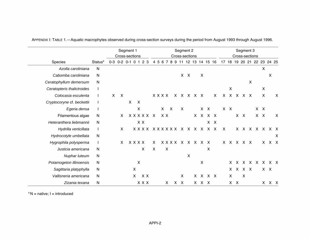
APPI-2

APPENDIX I: TABLE 1.—Aquatic macrophytes observed during cross-section surveys during the period from August 1993 through August 1996.

Segment 1 Segment 2 Segment 3Cross-sections Cross-sections Cross-sections

Species Statusa 0-3 0-2 0-1 0 1 2 3 4 5 6 7 8 9 11 12 13 14 15 16 17 18 19 20 21 22 23 24 25

Azolla caroliniana N X

Cabomba caroliniana N X X X X

Ceratophyllum demersum N X

Ceratopteris thalictroides I X X

Colocasia esculenta I X X X X X X X X X X X X X X X X X X X

Cryptocoryne cf. beckettii I X X

Egeria densa I X X X X X X X X X X

Filamentous algae N X X X X X X X X X X X X X X X X X X

Heteranthera liebmannii N X X X X

Hydrilla verticillata I X X X X X X X X X X X X X X X X X X X X X X X X X

Hydrocotyle umbellata N X

Hygrophila polysperma I X X X X X X X X X X X X X X X X X X X X X X X

Justicia americana N X X X X

Nuphar luteum N X

Potamogeton illinoensis N X X X X X X X X X X

Sagittaria platyphylla N X X X X X X X

Vallisneria americana N X X X X X X X X X X

Zizania texana N X X X X X X X X X X X X X X

a N = native; I = introduced

APPI-3

524

526

528

530

532

534

536

538

540

542

544

0.0

0.1

0.2

0.3

0 10 20 30 40 50 60 70 80 90 100 110 120 130 140 150

Ele

vatio

n (M

SL

ft)

Cur

rent

vel

ocity

(ft/

s)

Station (ft)

WSE 537.03

APPENDIX I: FIGURE 1.—Cross-section 0-3: Bottom profile, water surfaceelevation (WSE) and current velocity distribution illustrated for high, medium andlow streamflows. Mean depth and current velocity are reported with ranges inparentheses. This is pool mesohabitat in Segment 1 with silt substrate and sparseColocasia esculenta and Nuphar luteum.

Mean depth = 9.7 ft (0.0 - 12.0)

Mean velocity = 0.05 ft/s (0.00 - 0.13)

Cross-section 0-3

524

526

528

530

532

534

536

538

540

542

544

0.0

0.1

0.2

0.3E

leva

tion

(MS

L ft)

Cur

rent

vel

ocity

(ft/

s)

WSE 537.90

Mean depth = 9.8 ft (0.0 - 13.0)

Mean velocity = 0.06 ft/s (0.00 - 0.27)

9 May 1995

High Flow

524

526

528

530

532

534

536

538

540

542

544

0.0

0.1

0.2

0.3

Ele

vatio

n (M

SL

ft)

Cur

rent

vel

ocity

(ft/

s)

WSE 537.33

Mean depth = 9.9 ft (1.8 - 12.8)

Mean velocity = 0.01 ft/s (0.00 - 0.01)

29 June 1994

Medium Flow

21 August 1996

Low Flow

APPI-4

APPENDIX I: FIGURE 2.—Cross-section 0-2: Bottom profile, water surfaceelevation (WSE) and current velocity distribution illustrated for high, medium andlow streamflows. Mean depth and current velocity are reported with ranges inparentheses. This is run mesohabitat in Segment 1 with silt, clay, and sandsubstrate and sparse Colocasia esculenta, Hygrophila polysperma, Hydrillaverticillata, and filamentous algae.

528

530

532

534

536

538

540

542

544

0.0

0.2

0.4

0.6

0.8

1.0

1.2E

leva

tion

(MS

L ft)

Cur

rent

vel

ocity

(ft/

s)

Cross-section 0-2

WSE 538.07

Mean depth = 4.2 ft (0.0 - 6.7)

Mean velocity = 0.44 ft/s (0.00 - 1.19)

528

530

532

534

536

538

540

542

544

0.0

0.2

0.4

0.6

0.8

1.0

1.2

0 5 10 15 20 25 30 35 40 45 50 55 60 65 70

Ele

vatio

n (M

SL

ft)

Cur

rent

vel

ocity

(ft/

s)

Station (ft)

WSE 537.24

Mean depth = 3.24 ft (0.0 - 5.5)

Mean velocity = 0.34 ft/s (0.00 - 0.94)

9 May 1995

High Flow

528

530

532

534

536

538

540

542

544

0.0

0.2

0.4

0.6

0.8

1.0

1.2

Ele

vatio

n (M

SL

ft)

Cur

rent

vel

ocity

(ft/

s)

WSE 537.53

Mean depth = 4.15 ft (0.6 - 7.5)

Mean velocity = 0.33 ft/s (0.00 - 0.97)

10 June 1994

Medium Flow

22 Aug 1996

Low Flow

APPI-5

APPENDIX I: FIGURE 3.—Cross-section 0-1: Bottom profile, water surfaceelevation (WSE) and current velocity distribution illustrated for high, medium andlow streamflows. Mean depth and current velocity are reported with ranges inparentheses. This is run mesohabitat in Segment 1 with silt, clay and sandsubstrate and sparse Hygrophila polysperma, Cryptocoryne cf. beckettii andfilamentous algae.

Cross-section 0-1

532533534535536537538539540541542543544

0.0

0.2

0.4

0.6

0.8

1.0

1.2

1.4E

leva

tion

(MS

L ft)

Cur

rent

vel

ocity

(ft/

s)

Mean depth = 3.8 ft (0.5 - 5.8)

Mean velocity = 0.56 ft/s (0.00 - 1.38)

WSE 538.35

20 April 1995

High Flow

532533534535536537538539540541542543544

0.0

0.2

0.4

0.6

0.8

1.0

1.2

1.4

Ele

vatio

n (M

SL

ft)

Cur

rent

vel

ocity

(ft/

s)

Mean depth = 3.39 ft (0.0 - 5.3)

Mean velocity = 0.46 ft/s (0.00 - 1.26)

WSE 537.83

10 June 1994

Medium Flow

532533534535536537538539540541542543544

0.0

0.2

0.4

0.6

0.8

1.0

1.2

1.4

0 5 10 15 20 25 30 35 40 45 50 55 60 65

Ele

vatio

n (M

SL

ft)

Cur

rent

vel

ocity

(ft/

s)

Station (ft)

Mean depth = 2.86 ft (0.0 - 4.7)

Mean velocity = 0.36 ft/s (0.00 - 0.85)

WSE 537.39

22 August 1996

Low Flow

APPI-6

Cross-section 0

535

536

537

538

539

540

541

542

543

544

545

546

0.0

0.5

1.0

1.5

2.0

2.5

3.0

3.5E

leva

tion

(MS

L ft)

Cur

rent

vel

ocity

(ft/

s)

535

536

537

538

539

540

541

542

543

544

545

546

0.0

0.5

1.0

1.5

2.0

2.5

3.0

3.5

Ele

vatio

n (M

SL

ft)

Cur

rent

vel

ocity

(ft/

s)

WSE 538.66

WSE 538.40

Mean depth = 1.7 ft (0.0 - 2.9)

Mean velocity = 1.79 ft/s (0.00 - 3.32)

Mean depth = 1.5 ft (0.0 - 2.7)

Mean velocity = 1.65 ft/s (0.00 - 3.31)

APPENDIX I: FIGURE 4.—Cross-section 0: Bottom profile, water surface elevation(WSE) and current velocity distribution illustrated for high, medium and lowstreamflows. Mean depth and current velocity are reported with ranges inparentheses. This is fast shallow run mesohabitat, in Segment 1 with a mixed gravelsubstrate and sparse Hygrophila polysperma, Hydrilla verticillata, Vallisneriaamericana and filamentous algae.

9 August 1993

High Flow

11 May 1994

Medium Flow

535

536

537

538

539

540

541

542

543

544

545

546

0.0

0.5

1.0

1.5

2.0

2.5

3.0

3.5

0 5 10 15 20 25 30 35 40 45 50 55 60 65 70 75 80

Ele

vatio

n (M

SL

ft)

Cur

rent

vel

ocity

(ft/

s)

Station (ft)

WSE 537.80

Mean depth = 1.0 ft (0.0 - 1.6)

Mean velocity = 1.92 ft/s (0.00 - 3.37)

14 August 1996

Low Flow

APPI-7

Cross-section 1

534

535

536

537

538

539

540

541

542

543

0.0

0.5

1.0

1.5

2.0

2.5

3.0

Ele

vatio

n (M

SL

ft)

Cur

rent

vel

ocity

(ft/

s)

534

535

536

537

538

539

540

541

542

543

0.0

0.5

1.0

1.5

2.0

2.5

3.0

0 5 10 15 20 25 30 35 40 45 50 55

Ele

vatio

n (M

SL

ft)

Cur

rent

vel

ocity

(ft/

s)

Station (ft)

APPENDIX I: FIGURE 5.—Cross-section 1: Bottom profile, water surfaceelevation (WSE) and current velocity distribution illustrated for high, medium andlow streamflows. Mean depth and current velocity are reported with ranges inparentheses. This is run mesohabitat in Segment 1 with sand, fine gravel, andsilt substrate and sparse Cryptocoryne cf. beckettii, Hygrophila polysperma,Heteranthera liebmannii, Hydrilla verticillata and filamentous algae.

20 August 1993

Q = 194 ft /s3

534

535

536

537

538

539

540

541

542

543

0.0

0.5

1.0

1.5

2.0

2.5

3.0E

leva

tion

(MS

L ft)

Cur

rent

vel

ocity

(ft/

s)

WSE 538.78

Mean depth = 2.5 ft (0.0 - 4.0)

Mean velocity = 0.98 ft/s (0.00 - 2.45)

WSE 538.97

Mean depth = 2.3 ft (0.0 - 4.2)

Mean velocity = 1.36 ft/s (0.00 - 2.65)

WSE 538.22

Mean depth = 1.7 ft (0.0 - 2.8)

Mean velocity = 0.85 ft/s (0.00 - 1.69)

20 August 1993

High Flow

2 June 1994

Medium Flow

14 Aug 1996

Low Flow

APPI-8

APPENDIX I: FIGURE 6.—Cross-section 2: Bottom profile, water surfaceelevation (WSE) and current velocity distribution illustrated for high, mediumand low streamflows. Mean depth and current velocity are reported with rangesin parentheses. This is fast run mesohabitat in Segment 1 with sand, silt andclay substrate and Zizania texana, Vallisneria americana, Hygrophilapolysperma, Heteranthera liebmannii and Justicia americana.

Cross-section 2

536

537

538

539

540

541

542

543

544

545

0.0

0.2

0.4

0.6

0.8

1.0

1.2

1.4

1.6

1.8

2.0

Ele

vatio

n (M

SL

ft)

Cur

rent

vel

ocity

(ft/

s)

WSE 539.06

Mean depth = 1.9 ft (0.0 - 2.9)

Mean velocity = 0.81 ft/s (0.00 - 1.34)

2 June 1994

Medium flow

536

537

538

539

540

541

542

543

544

545

0.0

0.2

0.4

0.6

0.8

1.0

1.2

1.4

1.6

1.8

2.0E

leva

tion

(MS

L ft)

Cur

rent

vel

ocity

(ft/

s)

WSE 539.46

Mean depth = 2.2 ft (0.0 - 3.2)

Mean velocity = 0.77 ft/s (0.00 - 1.87)

20 August 1993

High Flow

536

537

538

539

540

541

542

543

544

545

0.0

0.2

0.4

0.6

0.8

1.0

1.2

1.4

1.6

1.8

2.0

0 5 10 15 20 25 30 35 40 45 50 55 60 65 70 75

Ele

vatio

n (M

SL

ft)

Cur

rent

vel

ocity

(ft/

s)

Station (ft)

WSE 538.53

Mean depth = 1.4 ft (0.0 - 2.3)

Mean velocity = 0.83 ft/s (0.00 - 1.54)

14 August 1996

Low Flow

APPI-9

APPENDIX I: FIGURE 7.—Cross-section 3: Bottom profile, water surfaceelevation (WSE) and current velocity distribution illustrated for high, mediumand low streamflows. Mean depth and current velocity are reported with rangesin parentheses. This is fast run mesohabitat in Segment 1 with sand and gravelsubstrate and Zizania texana, Vallisneria americana, Hydrilla verticillata andfilamentous algae.

Cross-section 3

537

538

539

540

541

542

543

544

545

546

0.0

0.5

1.0

1.5

2.0

2.5

3.0E

leva

tion

(MS

L ft)

Cur

rent

vel

ocity

(ft/

s)

537

538

539

540

541

542

543

544

545

546

0.0

0.5

1.0

1.5

2.0

2.5

3.0

Ele

vatio

n (M

SL

ft)

Cur

rent

vel

ocity

(ft/

s)

537

538

539

540

541

542

543

544

545

546

0.0

0.5

1.0

1.5

2.0

2.5

3.0

0 5 10 15 20 25 30 35 40 45 50 55

Ele

vatio

n (M

SL

ft)

Cur

rent

vel

ocity

(ft/

s)

Station (ft)

WSE 540.67

Mean depth = 2.0 ft (0.0 - 3.1)

Mean velocity = 1.14 ft/s (0.00 - 2.05)

WSE 540.30

Mean depth = 1.7 ft (0.0 - 2.6)

Mean velocity = 1.59 ft/s (0.00 - 2.31)

20 August 1993

High flow

2 June 1994

Medium Flow

WSE 539.94

Mean depth = 1.1 ft (0.0 - 2.0)

Mean velocity = 1.38 ft/s (0.00 - 2.58)14 August 1996

Low Flow

APPI-10

539

540

541

542

543

544

545

546

547

548

549

0.0

0.5

1.0

1.5

2.0

2.5

3.0

3.5

0 5 10 15 20 25 30 35 40 45 50 55 60 65 70 75

Ele

vatio

n (M

SL

ft)

Cur

rent

vel

ocity

(ft/

s)

Station (ft)

539

540

541

542

543

544

545

546

547

548

549

0.0

0.5

1.0

1.5

2.0

2.5

3.0

3.5

Ele

vatio

n (M

SL

ft)

Cur

rent

vel

ocity

(ft/

s)

539

540

541

542

543

544

545

546

547

548

549

0.0

0.5

1.0

1.5

2.0

2.5

3.0

3.5

Ele

vatio

n (M

SL

ft)

Cur

rent

Vel

ocity

(ft/

s)

APPENDIX I: FIGURE 8.—Cross-section 4: Bottom profile, water surfaceelevation (WSE) and current velocity distribution illustrated for high, medium andlow streamflows. Mean depth and current velocity are reported with ranges inparentheses. This is fast run mesohabitat in Segment 2 with sand and smallgravel substrate and Hydrilla verticillata, filamentous algae, Hygrophilapolysperma, Justicia americana and Colocasia esculenta.

Cross-section 4

WSE 541.53

Mean depth = 1.1 ft (0.0 - 2.0)

Mean velocity = 1.31 ft/s (0.00 - 2.88)

WSE 541.47

Mean depth = 1.1 ft (0.0 - 1.5)

Mean velocity = 2.05 ft/s (0.00 - 3.11)

14 August 1996

High Flow

18 August 1993

Medium Flow

WSE 541.45

Mean depth = 0.9 ft (0.0 - 1.7)

Mean velocity = 0.98 ft/s (0.00 - 2.65)

25 May 1994

Low flow

APPI-11

APPENDIX I: FIGURE 9.—Cross-section 5: Bottom profile, water surfaceelevation (WSE) and current velocity distribution illustrated for high, mediumand low streamflows. Mean depth and current velocity are reported with rangesin parentheses. This is riffle mesohabitat in Segment 2 with sand and mixedgravel and Hydrilla verticillata, Colocasia esculenta and Vallisneria americana.

Cross-section 5

541

542

543

544

545

546

547

548

0.0

0.5

1.0

1.5

2.0

2.5

Ele

vatio

n (M

SL

ft)

Cur

rent

vel

ocity

(ft/

s)

WSE 543.41

Mean depth = 1.1 ft (0.0 - 1.6)

Mean velocity = 1.04 ft/s (0.00 - 2.21)

541

542

543

544

545

546

547

548

0.0

0.5

1.0

1.5

2.0

2.5E

leva

tion

(MS

L ft)

Cur

rent

vel

ocity

(ft/

s)

WSE 543.51

Mean depth = 1.2 ft (0.0 - 1.7)

Mean velocity = 1.06 ft/s (0.00 - 2.10)

541

542

543

544

545

546

547

548

0.0

0.5

1.0

1.5

2.0

2.5

0 5 10 15 20 25 30 35 40 45 50 55 60 65 70 75

Ele

vatio

n (M

SL

ft)

Cur

rent

vel

ocity

(ft/

s)

Station (ft)

WSE 543.45

Mean depth = 1.2 ft (0.0 - 1.7)

Mean velocity = 0.66 ft/s (0.00 - 1.17)

14 August 1996

High Flow

11 August 1993

Medium Flow

25 May 1994

Low Flow

APPI-12

APPENDIX I: FIGURE 10.—Cross-section 6: Bottom profile, water surfaceelevation (WSE) and current velocity distribution illustrated for high, medium andlow streamflows. Mean depth and current velocity are reported with ranges inparentheses. This is riffle mesohabitat in Segment 2 with coarse and largegravel and some cobble substrate and sparse filamentous algae, Hydrillaverticillata and Colocasia esculenta.

Cross-section 6

543

544

545

546

547

548

549

0.0

0.5

1.0

1.5

2.0

2.5

3.0

3.5

4.0

4.5E

leva

tion

(MS

L ft)

Cur

rent

vel

ocity

(ft/

s)

543

544

545

546

547

548

549

0.0

0.5

1.0

1.5

2.0

2.5

3.0

3.5

4.0

4.5

0 5 10 15 20 25 30 35 40 45 50

Ele

vatio

n (M

SL

ft)

Cur

rent

vel

ocity

(ft/

s)

Station (ft)

WSE 544.61

Mean depth = 0.7 ft (0.0 - 0.9)

Mean velocity = 1.91 ft/s (0.00 - 4.13)

14 August 1996

High Flow

543

544

545

546

547

548

549

0.0

0.5

1.0

1.5

2.0

2.5

3.0

3.5

4.0

4.5

Ele

vatio

n (M

SL

ft)

Cur

rent

vel

ocity

(ft/

s)

WSE 544.65

Mean depth = 0.8 ft (0.0 - 1.2)

Mean velocity = 1.51 ft/s (0.00 - 3.46)

18 August 1993

Medium flow

WSE 544.51

Mean depth = 0.7 ft (0.0 - 1.0)

Mean velocity = 1.30 ft/s (0.00 - 3.63)

25 May 1994

Low flow

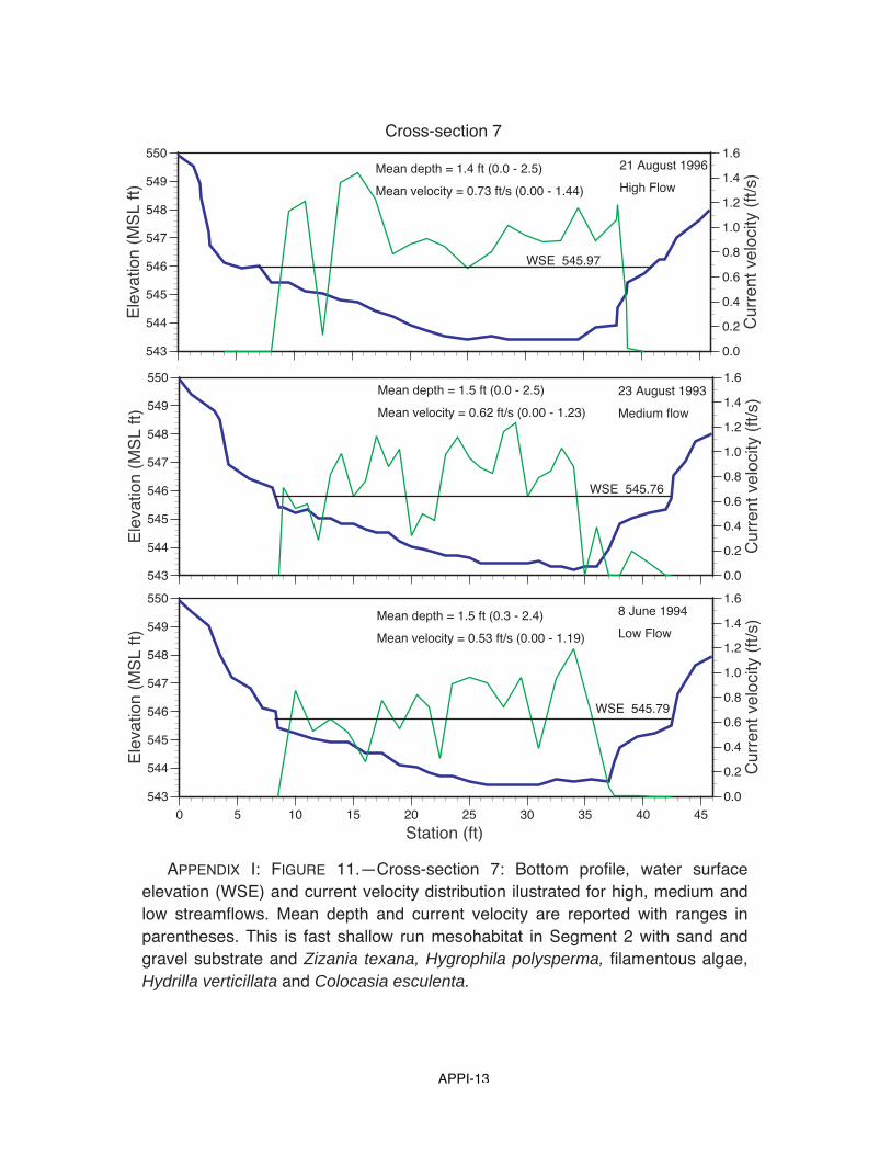
APPI-13

Cross-section 7

543

544

545

546

547

548

549

550

0.0

0.2

0.4

0.6

0.8

1.0

1.2

1.4

1.6

Ele

vatio

n (M

SL

ft)

Cur

rent

vel

ocity

(ft/

s)

WSE 545.97

Mean depth = 1.4 ft (0.0 - 2.5)

Mean velocity = 0.73 ft/s (0.00 - 1.44)

21 August 1996

High Flow

543

544

545

546

547

548

549

550

0.0

0.2

0.4

0.6

0.8

1.0

1.2

1.4

1.6

0 5 10 15 20 25 30 35 40 45

Ele

vatio

n (M

SL

ft)

Cur

rent

vel

ocit y

(ft/

s)

Station (ft)

Mean depth = 1.5 ft (0.3 - 2.4)

Mean velocity = 0.53 ft/s (0.00 - 1.19)

WSE 545.79

8 June 1994

Low Flow

543

544

545

546

547

548

549

550

0.0

0.2

0.4

0.6

0.8

1.0

1.2

1.4

1.6

Ele

vatio

n (M

SL

ft)

Cur

rent

vel

ocit y

(ft/

s)

WSE 545.76

Mean depth = 1.5 ft (0.0 - 2.5)

Mean velocity = 0.62 ft/s (0.00 - 1.23)

23 August 1993

Medium flow

APPENDIX I: FIGURE 11.—Cross-section 7: Bottom profile, water surfaceelevation (WSE) and current velocity distribution ilustrated for high, medium andlow streamflows. Mean depth and current velocity are reported with ranges inparentheses. This is fast shallow run mesohabitat in Segment 2 with sand andgravel substrate and Zizania texana, Hygrophila polysperma, filamentous algae,Hydrilla verticillata and Colocasia esculenta.

APPI-14

APPENDIX I: FIGURE 12.—Cross-section 8: Bottom profile, water surfaceelevation (WSE) and current velocity distribution illustrated for high, medium andlow streamflows. Mean depth and current velocity are reported with ranges inparentheses. This is pool mesohabitat in Segment 2 with silt, sand and claysubstrate and very sparse Hygrophila polysperma and Hydrilla verticillata.

Cross-section 8

536

538

540

542

544

546

548

550

552

554

556

0.0

0.1

0.2

0.3

0.4

0.5

0.6

0.7

0.8

0.9

0 5 10 15 20 25 30 35 40 45 50 55 60 65 70 75 80 85 90

Ele

vatio

n (M

SL

ft)

Cur

rent

vel

ocity

(ft/

s)

Station (ft)

WSE 546.30

Mean depth = 4.6 ft (0.2 - 9.0)

Mean velocity = 0.06 ft/s (0.00 - 0.58)

536

538

540

542

544

546

548

550

552

554

556

0.0

0.1

0.2

0.3

0.4

0.5

0.6

0.7

0.8

0.9

Ele

vatio

n (M

SL

ft)

Cur

rent

vel

ocity

(ft/

s)

WSE 546.18

Mean depth = 3.8 ft (0.4 - 8.6)

Mean velocity = 0.08 ft/s (0.00 - 0.47)

536

538

540

542

544

546

548

550

552

554

556

0.0

0.1

0.2

0.3

0.4

0.5

0.6

0.7

0.8

0.9

Ele

vatio

n (M

SL

ft)

Cur

rent

vel

ocity

(ft/

s)

WSE 546.32

Mean depth = 5.4 ft (0.0 - 8.7)

Mean velocity = 0.22 ft/s (0.00 - 0.55)

21 August 1996

High Flow

27 August 1993

Medium flow

8 June 1994

Low Flow

APPI-15

Cross-section 9

APPENDIX I: FIGURE 13.—Cross-section 9: Bottom profile, water surfaceelevation (WSE) and current velocity distribution illustrated for high, medium andlow streamflows. Mean depth and current velocity are reported with ranges inparentheses. This is slow deep run mesohabitat in Segment 2 with silt substrateand dense Hydrilla verticillata, Colocasia esculenta and Hygrophila polysperma.

544

545

546

547

548

549

550

551

552

553

554

555

0.0

0.1

0.2

0.3

0.4

0.5

0.6E

leva

tion

(MS

L ft)

Cur

rent

vel

ocity

(ft/

s)

25 August 1993

High flow

WSE 553.42

Mean depth = 5.0 ft (0.1 - 7.5)

Mean velocity = 0.32 ft/s (0.00 - 0.60)

544

545

546

547

548

549

550

551

552

553

554

555

0.0

0.1

0.2

0.3

0.4

0.5

0.6

Ele

vatio

n (M

SL

ft)

Cur

rent

vel

ocity

(ft/

s)

8 June 1994

Medium flow

WSE 553.27

Mean depth = 4.9 ft (0.0 - 7.5)

Mean velocity = 0.19 ft/s (0.00 - 0.49)

544

545

546

547

548

549

550

551

552

553

554

555

0.0

0.1

0.2

0.3

0.4

0.5

0.6

0 5 10 15 20 25 30 35 40 45

Ele

vatio

n (M

SL

ft)

Cur

rent

vel

ocity

(ft/

s)

Station (ft)

21 August 1996

Low Flow

WSE 553.38

Mean depth = 4.5 ft (0.0 - 7.6)

Mean velocity = 0.05 ft/s (0.00 - 0.12)

APPI-16

Cross-section 11

APPENDIX I: FIGURE 14.—Cross-section 11: Bottom profile, water surfaceelevation (WSE) and current velocity distribution illustrated for high, medium andlow streamflows. Mean depth and current velocity are reported with ranges inparentheses. This is run mesohabitat in Segment 2 with predominately silt andsand substrate and Zizania texana, Vallisneria americana, Hygrophila polyspermaand Colocasia esculenta.

548

549

550

551

552

553

554

555

556

557

558

559

0.0

0.1

0.2

0.3

0.4

0.5

0.6

0.7

0.8

0.9

Ele

vatio

n (M

SL

ft)

Cur

rent

vel

ocity

(ft/

s)

WSE 554.37

Mean depth = 2.9 ft (0.0 - 5.2)

Mean velocity = 0.30 ft/s (0.00 - 0.79)

11 August 1993

High Flow

548

549

550

551

552

553

554

555

556

557

558

559

0.0

0.1

0.2

0.3

0.4

0.5

0.6

0.7

0.8

0.9

Ele

vatio

n (M

SL

ft)

Cur

rent

vel

ocity

(ft/

s)

WSE 553.84

Mean depth = 2.4 ft (0.0 - 4.8)

Mean velocity = 0.26 ft/s (0.00 - 0.84)

6 June 1994

Medium Flow

548

549

550

551

552

553

554

555

556

557

558

559

0.0

0.1

0.2

0.3

0.4

0.5

0.6

0.7

0.8

0.9

0 10 20 30 40 50 60 70 80 90 100 110 120 130 140 150 160 170

Ele

vatio

n (M

SL

ft)

Cur

rent

vel

ocity

(ft/

s)

Station (ft)

WSE 553.54

Mean depth = 2.4 ft (0.0 - 4.4)

Mean velocity = 0.25 ft/s (0.00 - 0.73)

20 August 1996

Low Flow

APPI-17

539

541

543

545

547

549

551

553

555

557

559

-0.2

-0.1

0.0

0.1

0.2

0.3

0.4

0.5

0.6

Ele

vatio

n (M

SL

ft)

Cur

rent

vel

ocity

(ft/

s)

539

541

543

545

547

549

551

553

555

557

559

-0.2

-0.1

0

0.1

0.2

0.3

0.4

0.5

0.6

Ele

vatio

n (M

SL

ft)

Cur

rent

vel

ocity

(ft/

s)

539

541

543

545

547

549

551

553

555

557

559

-0.2

-0.1

0.0

0.1

0.2

0.3

0.4

0.5

0.6

0 10 20 30 40 50 60 70 80 90 100 110 120

Ele

vatio

n (M

SL

ft)

Cur

rent

vel

ocity

(ft/

s)

Station (ft)

WSE 553.99

WSE 553.76

WSE 553.66

Cross-section 12

Mean depth = 7.6 ft (0.0 - 13.5)

Mean velocity = 0.03 ft/s (0.00 - 0.19)

APPENDIX I: FIGURE 15.—Cross-section 12: Bottom profile, water surfaceelevation (WSE) and current velocity distribution illustrated for high, medium andlow streamflows. Mean depth and current velocity are reported with ranges inparentheses. This is pool mesohabitat in Segment 2 with silt, clay and sandsubstrate and Cabomba caroliniana, Hydrilla verticillata, Colocasia esculenta andHygrophila polysperma.

Mean depth = 8.0 ft (0.0 - 13.5)

Mean velocity = 0.06 ft/s (0.00 - 0.27)

Mean depth = 8.4 ft (0.0 - 14.1)

Mean velocity = 0.13 ft/s (0.00 - 0.55)

15 September 1993

High Flow

9 June 1994

Medium Flow

21 August 1996

Low Flow

APPI-18

551

552

553

554

555

556

557

558

559

560

0.0

0.5

1.0

1.5

2.0

2.5E

leva

tion

(MS

L ft)

Cur

rent

vel

ocity

(ft/

s)

551

552

553

554

555

556

557

558

559

560

0.0

0.5

1.0

1.5

2.0

2.5

Ele

vatio

n (M

SL

ft)

Cur

rent

vel

ocity

(ft/

s)

551

552

553

554

555

556

557

558

559

560

0.0

0.5

1.0

1.5

2.0

2.5

0 5 10 15 20 25 30 35 40 45 50 55 60 65 70 75 80 85 90

Ele

vatio

n (M

SL

ft)

Cur

rent

vel

ocity

(ft/

s)

Station (ft)

WSE 553.82

WSE 553.97

WSE 554.51

Cross-section 13

Mean depth = 1.8 ft (0.0 - 2.9)

Mean velocity = 1.15 ft/s (0.00 - 1.85)

APPENDIX I: FIGURE 16.—Cross-section 13: Bottom profile, water surfaceelevation (WSE) and current velocity distribution illustrated for high, medium andlow streamflows. Mean depth and current velocity are reported with ranges inparentheses. This is fast shallow run mesohabitat in Segment 2 with sand, graveland bedrock substrate and Zizania texana, Vallisneria americana, Hygrophilapolysperma, filamentous algae and Colocasia esculenta.

Mean depth = 1.5 ft (0.7 - 3.0)

Mean velocity = 1.25 ft/s (0.00 - 2.40)

Mean depth = 1.4 ft (0.0 - 2.2)

Mean velocity = 0.79 ft/s (0.00 - 1.33)

11 August 1993

High flow

24 May 1994

Medium Flow

14 August 1996

Low Flow

APPI-19

548549550551552553554555556557558559560561

0.0

0.2

0.4

0.6

0.8

1.0

1.2

1.4

1.6

Ele

vatio

n (M

SL

ft)

Cur

rent

Vel

ocity

(ft/

s)

548549550551552553554555556557558559560561

0.0

0.2

0.4

0.6

0.8

1.0

1.2

1.4

1.6

Ele

vatio

n (M

SL

ft)

Cur

rent

vel

ocity

(ft/

s)

548549550551552553554555556557558559560561

0.0

0.2

0.4

0.6

0.8

1.0

1.2

1.4

1.6

0 5 10 15 20 25 30 35 40 45 50 55 60 65 70 75

Ele

vatio

n (M

SL

ft)

Cur

rent

Vel

ocity

(ft/

s)

Station (ft)

WSE 554.51

WSE 554.02

WSE 553.49

Mean depth = 3.39 ft (0.0 - 5.3)

Mean velocity = 0.46 ft/s (0.00 - 1.26)

APPENDIX I: FIGURE 17.—Cross-section 14: Bottom profile, water surfaceelevation (WSE) and current velocity distribution illustrated for high, medium and lowstreamflows. Mean depth and current velocity are reported with ranges inparentheses. This is run mesohabitat in Segment 2 with sand and silt substrateand Zizania texana, Cabomba caroliniana, Colocasia esculenta, Hygrophilapolysperma and Hydrilla verticillata.

Mean depth = 3.39 ft (0.0 - 5.3)

Mean velocity = 0.46 ft/s (0.00 - 1.26)

Mean depth = 3.39 ft (0.0 - 5.3)

Mean velocity = 0.46 ft/s (0.00 - 1.26)

Cross-section 14

25 August 1993

High Flow

6 June 1994

Medium Flow

19 August 1996

Low Flow

APPI-20

552

553

554

555

556

557

558

559

0.0

0.5

1.0

1.5

2.0

2.5

3.0E

leva

tion

(MS

L ft)

Cur

rent

vel

ocity

(ft/

s)

552

553

554

555

556

557

558

559

0.0

0.5

1.0

1.5

2.0

2.5

3.0

Ele

vatio

n (M

SL

ft)

Cur

rent

vel

ocity

(ft/

s)

552

553

554

555

556

557

558

559

0.0

0.5

1.0

1.5

2.0

2.5

3.0

0 5 10 15 20 25 30 35 40 45 50 55 60 65 70 75 80 85 90 95

Ele

vatio

n (M

SL

ft)

Cur

rent

vel

ocity

(ft/

s)

Station (ft)

WSE 554.95

WSE 554.56

WSE 554.07

Mean depth = 0.9 ft (0.1 - 1.6)

Mean velocity = 1.08 ft/s (0.00 - 2.64)

APPENDIX I: FIGURE 18.—Cross-section 15: Bottom profile, water surfaceelevation (WSE) and current velocity distribution illustrated for high, medium andlow streamflows. Mean depth and current velocity are reported with ranges inparentheses. This is fast run mesohabitat in Segment 2 with sand and mixedgravel substrate and Zizania texana, Vallisneria americana, Hygrophila polyspermaand Hydrilla verticillata.

Mean depth = 1.5 ft (0.0 - 2.5)

Mean velocity = 1.13 ft/s (0.00 - 2.20)

Mean depth = 1.2 ft (0.0 - 2.3)

Mean velocity = 1.08 ft/s (0.00 - 2.32)

Cross-section 15

10 August 1993

High Flow

24 May 1994

Medium flow

13 August 1996

Low Flow

APPI-21

553

554

555

556

557

558

559

560

561

0.0

0.5

1.0

1.5

2.0

2.5

3.0

3.5

4.0

Ele

vatio

n (M

SL

ft)

Cur

rent

vel

ocity

(ft/

s)

553

554

555

556

557

558

559

560

561

0.0

0.5

1.0

1.5

2.0

2.5

3.0

3.5

4.0E

leva

tion

(MS

L ft)

Cur

rent

vel

ocity

(ft/

s)

553

554

555

556

557

558

559

560

561

0.0

0.5

1.0

1.5

2.0

2.5

3.0

3.5

4.0

0 5 10 15 20 25 30 35 40 45 50 55 60 65 70 75 80 85 90 95 100

Ele

vatio

n (M

SL

ft)

Cur

rent

vel

ocity

(ft/

s)

Station (ft)

WSE 555.31

WSE 555.25

WSE 554.75

Cross-section 16

Mean depth = 1.0 ft (0.0 - 1.9)

Mean velocity = 1.98 ft/s (0.00 - 3.26)

APPENDIX I: FIGURE 19.—Cross-section 16: Bottom profile, water surfaceelevation (WSE) and current velocity distribution illustrated for high, medium andlow streamflows. Mean depth and current velocity are reported with ranges inparentheses. This is riffle mesohabitat in Segment 2 with mixed gravel, sand andcobble substrate and sparse Colocasia esculenta, Hydrilla verticillata, filamentousalgae andVallisneria americana.

Mean depth = 0.9 ft (0.0 - 1.0)

Mean velocity = 0.46 ft/s (0.00 - 1.26)

Mean depth = 0.5 ft (0.0 - 1.1)

Mean velocity = 1.29 ft/s (0.00 - 3.89)

29 October 1997

High Flow

24 May 1994

Medium Flow

13 August 1996

Low Flow

APPI-22

551552553554555556557558559560561562563564

0.0

0.1

0.2

0.3

0.4

0.5

0.6

Ele

vatio

n (M

SL

ft)

Cur

rent

vel

ocity

(ft/

s)

WSE 560.26

Cross-section 17

Mean depth = 4.0 ft (0.0 - 8.2)

Mean velocity = 0.20 ft/s (0.00 - 0.55)

APPENDIX I: FIGURE 20.—Cross-section 17: Bottom profile, water surfaceelevation (WSE) and current velocity distribution illustrated for high, medium andlow streamflows. Mean depth and current velocity are reported with ranges inparentheses. This is pool mesohabitat in Segment 3 with mostly silt substrate andsome sand and dense Egeria densa, Hydrilla verticillata, Colocasia esculenta andHygrophila polysperma.

24 August 1993

High Flow

551552553554555556557558559560561562563564

0.0

0.1

0.2

0.3

0.4

0.5

0.6

0 10 20 30 40 50 60 70 80 90 100 110 120 130 140

Ele

vatio

n (M

SL

ft)

Cur

rent

vel

ocity

(ft/

s)

Station (ft)

WSE 559.76

Mean depth = 3.3 ft (0.0 - 7.4)

Mean velocity = 0.12 ft/s (0.00 - 0.27)

15 August 1996

Low Flow

551552553554555556557558559560561562563564

0.0

0.1

0.2

0.3

0.4

0.5

0.6

Ele

vatio

n (M

SL

ft)

Cur

rent

vel

ocity

(ft/

s)

WSE 560.31

Mean depth = 4.0 ft (0.0 - 8.0)

Mean velocity = 0.08 ft/s (0.00 - 0.26)

3 June 1994

Medium Flow

APPI-23

557

558

559

560

561

562

563

564

0.0

0.1

0.2

0.3

0.4

0.5

0.6

0.7

0.8

0.9E

leva

tion

(MS

L ft)

Cur

rent

vel

ocity

(ft/

s)

557

558

559

560

561

562

563

564

0.0

0.1

0.2

0.3

0.4

0.5

0.6

0.7

0.8

0.9

Ele

vatio

n (M

SL

ft)

Cur

rent

vel

ocity

(ft/

s)

557

558

559

560

561

562

563

564

0.0

0.1

0.2

0.3

0.4

0.5

0.6

0.7

0.8

0.9

0 5 10 15 20 25 30 35 40 45 50 55 60 65 70 75 80 85 90 95 100 105

Ele

vatio

n (M

SL

ft)

Cur

rent

vel

ocity

(ft/

s)

Station (ft)

WSE 560.48

WSE 560.38

WSE 559.90

Mean depth = 1.4 ft (0.0 - 2.8)

Mean velocity = 0.12 ft/s (0.00 - 0.89)

APPENDIX I: FIGURE 21.—Cross-section 18: Bottom profile, water surfaceelevation (WSE) and current velocity distribution illustrated for high, medium andlow streamflows. Mean depth and current velocity are reported with ranges inparentheses. This is slow run mesohabitat in Segment 3 with silt substrate andZizania texana, Hygrophila polysperma, Colocasia esculenta, Vallisneria americanaand Sagittaria platyphylla.

Mean depth = 1.4 ft (0.0 - 2.8)

Mean velocity = 0.07 ft/s (0.00 - 0.34)

Mean depth = 1.3 ft (0.0 - 2.5)

Mean velocity = 0.05 ft/s (0.00 - 0.16)

Cross-section 18

26 August 1993

High Flow

31 May 1994

Medium Flow

15 August 1996

Low Flow

APPI-24

557

558

559

560

561

562

563

564

565

566

0.0

0.2

0.4

0.6

0.8

1.0

1.2

1.4E

leva

tion

(MS

L ft)

Cur

rent

vel

ocity

(ft/

s)

557

558

559

560

561

562

563

564

565

566

0.0

0.2

0.4

0.6

0.8

1.0

1.2

1.4

Ele

vatio

n (M

SL

ft)

Cur

rent

vel

ocity

(ft/

s)557

558

559

560

561

562

563

564

565

566

0.0

0.2

0.4

0.6

0.8

1.0

1.2

1.4

0 10 20 30 40 50 60 70 80 90 100 110 120 130 140 150 160 170 180 190 200 210 220

Ele

vatio

n (M

SL

ft)

Cur

rent

vel

ocity

(ft/

s)

Station (ft)

WSE 560.71

WSE 560.49

WSE 559.97

Mean depth = 1.5 ft (0.0 - 3.4)

Mean velocity = 0.19 ft/s (0.00 - 0.85)

APPENDIX I: FIGURE 22.—Cross-section 19: Bottom profile, water surfaceelevation (WSE) and current velocity distribution illustrated for high, medium andlow streamflows. Mean depth and current velocity are reported with ranges inparentheses. This cross-section in Segment 3 represents two mesohabitat types,both with silt and sand substrates. River-left is a slow shallow run with Zizaniatexana, Hygrophila polysperma and Sagittaria platyphylla. River-right is a run withZizania texana, Sagittaria platyphylla, Hydrilla verticillata and Hygrophilapolysperma.

Mean depth = 1.6 ft (0.0 - 3.4)

Mean velocity = 0.34 ft/s (0.00 - 1.23)

Mean depth = 1.1 ft (0.4 - 2.3)

Mean velocity = 0.46 ft/s (0.01 - 0.95)

Cross-section 19

10 August 1993

High Flow

31 May 1994

Medium Flow

15 August 1996

Low Flow

APPI-25

557

558

559

560

561

562

563

564

565

0.0

0.5

1.0

1.5

2.0

2.5

3.0

3.5E

leva

tion

(MS

L ft)

Cur

rent

vel

ocity

(ft/

s)

557

558

559

560

561

562

563

564

565

0.0

0.5

1.0

1.5

2.0

2.5

3.0

3.5

Ele

vatio

n (M

SL

ft)

Cur

rent

vel

ocit y

(ft/

s)557

558

559

560

561

562

563

564

565

0.0

0.5

1.0

1.5

2.0

2.5

3.0

3.5

0 10 20 30 40 50 60 70 80 90 100 110 120 130

Ele

vatio

n (M

SL

ft)

Cur

rent

vel

ocit y

(ft/

s)

Station (ft)

WSE 560.59

WSE 560.81

WSE 560.40

Mean depth = 1.3 ft (0.0 - 2.6)

Mean velocity = 0.77 ft/s (0.00 - 2.45)

APPENDIX I: FIGURE 23.—Cross-section 20: Bottom profile, water surfaceelevation (WSE) and current velocity distribution illustrated for high, medium andlow streamflows. Mean depth and current velocity are reported with ranges inparentheses. This cross-section in Segment 3 represents two habitat types. River-right is a slow shallow run. River-left is a fast run. Both habitats have silt, sand andclay substrates and Hygrophila polysperma, Hydrilla verticillata, Sagittariaplatyphylla and Vallisneria americana.

Cross-section 20

Mean depth = 0.8 ft (0.0 - 1.8)

Mean velocity = 0.83 ft/s (0.00 - 2.14)

Mean depth = 1.3 ft (0.0 - 2.8)

Mean velocity = 0.58 ft/s (0.00 - 3.27)

10-Aug-1993

High Flow

23-May-1994

Medium Flow

13-Aug-1996

Low Flow

APPI-26

Cross-section 21

APPENDIX I: FIGURE 24.—Cross-section 21: Bottom profile, water surfaceelevation (WSE) and current velocity distribution illustrated for high, medium andlow streamflows. Mean depth and current velocity are reported with ranges inparentheses. This cross-section in Segment 3 represents two types ofmesohabitats. Fast run exists on river right, in contrast to slow run on river left.Both habitats have primarily silt substrate with some sand and Hydrilla verticillata,Sagiittaria platyphylla and Colocasia esculenta.

555

556

557

558

559

560

561

562

563

564

565

0.0

0.1

0.2

0.3

0.4

0.5

0.6

0.7

0.8

0.9E

leva

tion

(MS

L ft)

Cur

rent

vel

ocity

(ft/

s)

WSE 561.47

Mean depth = 3.1 ft (0.0 - 5.4)

Mean velocity = 0.15 ft/s (0.00 - 0.86)

555

556

557

558

559

560

561

562

563

564

565

0.0

0.1

0.2

0.3

0.4

0.5

0.6

0.7

0.8

0.9

Ele

vatio

n (M

SL

ft)

Cur

rent

vel

ocity

(ft/

s)

WSE 561.25

Mean depth = 3.14 ft (0.0 - 5.5)

Mean velocity = 0.17 ft/s (0.00 - 0.64)

555

556

557

558

559

560

561

562

563

564

565

0.0

0.1

0.2

0.3

0.4

0.5

0.6

0.7

0.8

0.9

0 5 10 15 20 25 30 35 40 45 50 55 60 65 70 75 80 85 90 95 100 105

Ele

vatio

n (M

SL

ft)

Cur

rent

vel

ocity

(ft/

s)

Station (ft)

WSE 560.79

Mean depth = 2.9 ft (0.0 - 4.8)

Mean velocity = 0.23 ft/s (0.00 - 0.59)

24 August 1993

High Flow

3 June 1994

Medium Flow

15 August 1996

Low Flow

APPI-27

556

557

558

559

560

561

562

563

564

565

566

0.0

0.2

0.4

0.6

0.8

1.0

1.2

1.4

Ele

vatio

n (M

SL

ft)

Cur

rent

vel

ocity

(ft/

s)

556

557

558

559

560

561

562

563

564

565

566

0.0

0.2

0.4

0.6

0.8

1.0

1.2

1.4

Ele

vatio

n (M

SL

ft)

Cur

rent

vel

ocity

(ft/

s)

556

557

558

559

560

561

562

563

564

565

566

0.0

0.2

0.4

0.6

0.8

1.0

1.2

1.4

0 5 10 15 20 25 30 35 40 45 50 55 60 65 70 75 80 85 90 95 100105110115120

Ele

vatio

n (M

SL

ft)

Cur

rent

vel

ocity

(ft/

s)

Station (ft)

Mean depth = 2.29 ft (0.0 - 3.8)

Mean velocity = 0.43 ft/s (0.00 - 1.08)

APPENDIX I: FIGURE 25.—Cross-section 22: Bottom profile, water surfaceelevation (WSE) and current velocity distribution illustrated for high, medium andlow streamflow discharges. Mean depth and current velocity are reported withranges in parentheses. This is slow run mesohabitat in Segment 3 with mixedgravel and sand substrate and Hydrilla verticillata, Egeria densa, Potamogetonillinoensis and filamentous algae.

WSE 561.66

WSE 561.43

WSE 560.85

Mean depth = 1.87 ft (0.0 - 3.5)

Mean velocity = 0.61 ft/s (0.00 - 1.40)

Mean depth = 1.74 ft (0.3 - 3.2)

Mean velocity = 0.36 ft/s (0.00 - 0.97)

Cross-section 22

23 August 1993

High flow

18 May 1994

Medium Flow

13 August 1996

Low Flow

APPI-28

APPENDIX I: FIGURE 26.—Cross-section 23: Bottom profile, water surfaceelevation (WSE) and current velocity distribution illustrated for high, mediumand low streamflows. Mean depth and current velocity are reported with rangesin parentheses. This is run mesohabitat in Segment 3 with silt and some claysubstrate and dense Potamogeton illinoensis, Hydrilla verticillata, Sagittariaplatyphylla, Hygrophila polysperma, and sparse Zizania texana.

Cross-section 23

558559560561562563564565566567568569

0.0

0.2

0.4

0.6

0.8

1.0

1.2

1.4E

leva

tion

(MS

L ft)

Cur

rent

vel

ocity

(ft/

s)

WSE 562.04

Mean depth = 2.2 ft (0.5 - 3.5)

Mean velocity = 0.43 ft/s (0.00 - 1.36)

18 August 1993

High Flow

558559560561562563564565566567568569

0.0

0.2

0.4

0.6

0.8

1.0

1.2

1.4

Ele

vatio

n (M

SL

ft)

Cur

rent

vel

ocity

(ft/

s)

WSE 561.76

Mean depth = 1.9 ft (0.0 - 3.4)

Mean velocity = 0.31 ft/s (0.00 - 1.25)

23 May 1994

Medium Flow

558559560561562563564565566567568569

0.0

0.2

0.4

0.6

0.8

1.0

1.2

1.4

0 10 20 30 40 50 60 70 80 90 100 110 120 130 140 150 160 170 180

Ele

vatio

n (M

SL

ft)

Cur

rent

vel

ocity

(ft/

s)

Station (ft)

WSE 561.35

Mean depth = 1.5 ft (0.0 - 2.5)

Mean velocity = 0.16 ft/s (0.00 - 0.69)

13 August 1996

Low Flow

APPI-29

558

559

560

561

562

563

564

565

566

567

0.0

0.5

1.0

1.5

2.0

2.5

3.0E

leva

tion

(MS

L ft)

Cur

rent

vel

ocity

(ft/

s)

WSE 562.76

558

559

560

561

562

563

564

565

566

567

0.0

0.5

1.0

1.5

2.0

2.5

3.0

Ele

vatio

n (M

SL

ft)

Cur

rent

vel

ocity

(ft/

s)

558

559

560

561

562

563

564

565

566

567

0.0

0.5

1.0

1.5

2.0

2.5

3.0

0 5 10 15 20 25 30 35 40 45 50 55 60 65 70 75 80 85 90

Ele

vatio

n (M

SL

ft)

Cur

rent

vel

ocity

(ft/

s)

Station (ft)

WSE 562.42

WSE 561.90

Mean depth = 2.0 ft (0.0 - 4.0)

Mean velocity = 0.71 ft/s (0.00 - 2.13)

APPENDIX I: FIGURE 27.—Cross-section 24: Bottom profile, water surfaceelevation (WSE) and current velocity distribution illustrated for high, medium andlow streamflows. Mean depth and current velocity are reported with ranges inparentheses. This is run mesohabitat in Segment 3 with sand, gravel and siltsubstrate and Zizania texana, Potamogeton illinoensis, Hydrilla verticillata andHygrophila polysperma.

Mean depth = 2.38 ft (0.0 - 4.3)

Mean velocity = 0.98 ft/s (0.00 - 2.54)

Mean depth = 1.5 ft (0.0 - 2.9)

Mean velocity = 0.68 ft/s (0.00 - 2.33)

Cross-section 24

23 August 1993

High Flow

18 May 1994

Medium Flow

13 August 1996

Low Flow

APPI-30

560

561

562

563

564

565

566

567

0.0

0.5

1.0

1.5

2.0

2.5

3.0

3.5

4.0E

leva

tion

(MS

L ft)

Cur

rent

vel

ocity

(ft/

s)

560

561

562

563

564

565

566

567

0.0

0.5

1.0

1.5

2.0

2.5

3.0

3.5

4.0

Ele

vatio

n (M

SL

ft)

Cur

rent

vel

ocity

(ft/

s)

560

561

562

563

564

565

566

567

0.0

0.5

1.0

1.5

2.0

2.5

3.0

3.5

4.0

0 5 10 15 20 25 30 35 40 45 50 55 60 65 70 75 80 85 90 95 100 105

Ele

vatio

n (M

SL

ft)

Cur

rent

vel

ocity

(ft/

s)

Station (ft)

WSE 562.98

WSE 562.60

WSE 561.98

Mean depth = 1.4 ft (0.0 - 2.2)

Mean velocity = 2.25 ft/s (0.00 - 3.57)

APPENDIX I: FIGURE 28.—Cross-section 25: Bottom profile, water surfaceelevation (WSE) and current velocity distribution illustrated for high, medium andlow streamflows. Mean depth and current velocity are reported with ranges inparentheses. This is a fast shallow run mesohabitat in Segment 3 with sand andmixed gravel substrate and Zizania texana, Potamogeton illinoensis, Hygrophilapolysperma and Colocasia esculenta.

Mean depth = 1.1 ft (0.0 - 1.9)

Mean velocity = 1.84 ft/s (0.00 - 3.21)

Mean depth = 0.9 ft (0.0 - 1.5)

Mean velocity = 1.76 ft/s (0.00 - 2.91)

Cross-section 25

9 August 1993

High Flow

11 May 1994

Medium Flow

13 August 1996

Low Flow

APPII-1

Appendix IIBiology

APPII-2

APPENDIX II: TABLE 1.—Aquatic macrophytes identified in the 43 biogrid samples.Vegetation type Statusa Fast deep run Fast shallow run Fast run Riffle Fast run/Slow run Run Slow run Slow deep run Pool Backwater

Amblystegium riparium N 23 1 38 1Azolla caroliniana N 28 2

Cabomba caroliniana N 1 25 19 4 65 29Ceratophyllum demersum N 7 1 2

Filamentous algae N 31 3 25 52 5 103 4 70 144Heteranthera liebmannii N 3 2 4 2 8 16 13 4 3

Hydrocotyle umbellata N 5 3 7 3Justicia americana N 10

Ludwigia repens N 1 8 1Myriophyllum heterophyllum N 2 2

Nuphar luteum N 8 18 7Pistia stratiotes N 1 1 5 6 8 14

Potamogeton illinoensis N 119 214 99 44 2Riccia fluitans N 26 4 7 2 1

Sagittaria platyphylla N 76 9 54 15 20Vallisneria americana N 10 1 5 20 5 2

Zizania texana N 5 17 2 38 2 6Ceratopteris thalictroides I 3 4

Colocasia esculenta I 3 7 37 21 44 68 24 66 50 66Cryptocoryne cf. beckettii I 6

Egeria densa I 81 8 150 15 35Eichhornia crassipes I 2 15 15 16 5 3 5

Hydrilla verticillata I 16 31 58 23 124 147 75 93 156 7Hygrophila polysperma I 1 13 68 22 173 206 142 69 97 24

36 60 126 83 216 296 246 559 391 455 13 0 5 1 23 13 387 137 34 4 7 6 10 12 11 7 14 43 4 3 4 5 5 6 5 5 531 7 122 66 214 231 84 83 199 32

86.11 11.67 96.83 79.52 99.07 78.04 34.15 14.85 50.90 71.1116 46 111 49 215 271 230 152 195 37

44.44 76.67 88.10 59.04 99.54 91.55 93.50 27.19 49.87 82.22

aN = Native; I = introduced

Number of cells sampledCells without vegetation

Cells with introduced speciesPercent cells with introduced species

Number of native speciesNumber of introduced speciesCells with native speciesPercent cells with native species

APPII-3

APPENDIX II: TABLE 2.—Aquatic macrophytes identified in the six Zizania texana biogrid samples.

Vegetation type Statusa Fast run Run Slow runCabomba caroliniana N 7

Filamentous algae N 53 72Heteranthera liebmannii N 21 15 1

Hydrocotyle umbellata N 2Justicia americana N 2

Ludwigia repens N 3Potamogeton illinoensis N 20 44

Sagittaria platyphylla N 35 18Vallisneria americana N 11 14 4

Zizania texana N 43 85 18Colocasia esculenta I 18 22 8

Egeria densa I 1 8Eichhornia crassipes I 2

Hydrilla verticillata I 85 112 10Hygrophila polysperma I 64 83 20

109 162 240 2 09 6 44 3 5

43 85 1839.45 52.47 75.00104 150 23

95.41 92.59 95.83106 133 24

97.25 82.10 100.00

a N = native; I = introduced

Cells with Zizania texana

Number of native speciesNumber of introduced species

Number of cells sampledCells without vegetation

Percent cells with Zizania texana

Percent cells with introduced species

Cells with native speciesPercent cells with native species Cells with introduced species

APPII-4

APPENDIX II: TABLE 3.—Aquatic macrophyte associations as observed in the 43 bio-grid samples. Note: This table is to be read by column (top to bottom).

Amblystegium Azolla Cabomba Ceratophyllum Ceratopteris Colocasia Cryptocoryne Egeria Eichornia Fil. Algae Heteranthera Hydrilla Hydrocotyle Hygrophila Justicia Ludwigia Myriophyllum Nuphar Pistia Potamogeton Riccia Sagittaria Vallisneria Zizania

Number of cells with species 63 30 144 10 7 356 6 289 61 438 57 730 18 815 10 10 4 34 35 478 40 174 43 70

Total # cells sampled 2058 2058 2058 2058 2058 2058 2058 2058 2058 2058 2058 2058 2058 2058 2058 2058 2058 2058 2058 2058 2058 2058 2058 2058

% of total cells with species 3.06 1.46 7.00 0.49 0.34 17.30 0.29 14.04 2.96 21.28 2.77 35.47 0.87 39.60 0.49 0.49 0.19 1.65 1.70 23.23 1.94 8.45 2.09 3.40

Frequency of Occurrencea L L M L L M L M L H L H L H L L L L L H L M L L

Amblystegium riparium 0.00 0.00 0.00 0.00 3.09 0.00 0.00 0.00 13.01 7.02 2.74 0.00 0.12 0.00 0.00 0.00 0.00 0.00 0.00 0.00 0.00 0.00 5.71

Azolla caroliniana 0.00 0.00 0.00 0.00 3.65 0.00 0.00 13.11 1.14 3.51 0.55 0.00 3.68 0.00 0.00 0.00 0.00 2.86 6.28 25.00 0.00 6.98 0.00

Cabomba caroliniana 0.00 0.00 30.00 100.00 17.42 0.00 9.69 4.92 9.59 5.26 10.41 0.00 11.41 0.00 0.00 25.00 44.12 34.29 0.00 2.50 0.57 6.98 7.14

Ceratophyllum demersum 0.00 0.00 2.08 0.00 0.28 0.00 2.77 0.00 0.00 0.00 0.27 0.00 0.86 0.00 0.00 0.00 0.00 0.00 0.00 2.50 0.00 2.33 0.00

Ceratopteris thalictroides 0.00 0.00 4.86 0.00 1.97 0.00 1.04 0.00 0.00 0.00 0.00 0.00 0.61 0.00 0.00 0.00 0.00 8.57 0.00 0.00 0.00 0.00 0.00

Colocasia esculenta 17.46 26.67 43.06 10.00 100.00 0.00 14.88 27.87 19.86 29.82 25.34 66.67 27.48 0.00 10.00 25.00 26.47 57.14 18.83 30.00 20.11 51.16 0.00

Cryptocoryne cf. beckettii 0.00 0.00 0.00 0.00 0.00 0.00 0.00 0.00 0.00 0.00 0.00 0.00 0.00 0.00 0.00 0.00 0.00 0.00 0.00 0.00 0.00 0.00 0.00

Egeria densa 0.00 0.00 19.44 80.00 42.86 12.08 0.00 16.39 6.16 21.05 12.05 0.00 27.48 0.00 40.00 50.00 5.88 2.86 19.04 17.50 14.37 4.65 2.86

Eichhornia crassipes 0.00 26.67 2.08 0.00 0.00 4.78 0.00 3.46 0.68 3.51 2.05 5.56 5.15 0.00 0.00 0.00 2.94 31.43 7.74 42.50 6.90 6.98 1.43

Filamentous algae 90.48 16.67 28.47 0.00 0.00 21.63 0.00 9.34 4.92 31.58 34.38 27.78 17.91 0.00 0.00 25.00 5.88 22.86 5.86 0.00 8.05 32.56 65.71

Heteranthera liebmannii 6.35 6.67 2.08 0.00 0.00 4.78 0.00 4.15 3.28 4.11 3.56 0.00 4.29 3.00 0.00 0.00 0.00 0.00 2.93 2.50 2.30 6.98 7.14

Hydrilla verticillata 31.75 13.33 52.78 20.00 0.00 51.97 0.00 30.45 24.59 59.36 45.61 38.89 41.60 0.00 80.00 50.00 38.24 20.00 46.86 37.50 35.06 51.16 72.86

Hydrocotyle umbellata 0.00 0.00 0.00 0.00 0.00 3.37 0.00 0.00 1.64 1.14 0.00 0.96 0.86 10.00 0.00 0.00 0.00 5.71 0.42 0.00 1.15 0.00 0.00

Hygrophila polysperma 1.59 100.00 64.58 70.00 71.43 62.92 0.00 77.51 68.85 35.16 61.40 46.44 38.89 0.00 60.00 100.00 23.53 31.43 73.64 77.50 77.01 83.72 50.00

Justicia americana 0.00 0.00 0.00 0.00 0.00 0.00 0.00 0.00 0.00 0.00 1.75 0.14 0.00 0.49 0.00 0.00 0.00 0.00 0.00 0.00 0.00 0.00 0.00

Ludwigia repens 0.00 0.00 0.00 0.00 0.00 0.28 0.00 1.38 0.00 0.00 0.00 1.10 0.00 0.74 3.00 0.00 0.00 0.00 1.88 0.00 0.00 2.33 0.00

Myriophyllum spp. 0.00 0.00 0.69 0.00 0.00 0.28 0.00 0.69 0.00 0.23 0.00 0.27 0.00 0.49 0.00 0.00 0.00 0.00 0.21 0.00 0.57 2.33 0.00

Nuphar luteum 0.00 0.00 10.42 0.00 0.00 2.53 0.00 0.69 1.64 0.46 0.00 1.78 0.00 0.98 0.00 0.00 0.00 11.43 0.00 0.00 0.00 0.00 0.00

Pistia stratiotes 0.00 3.33 8.33 0.00 42.86 5.62 0.00 0.35 18.03 1.83 0.00 0.96 11.11 1.35 0.00 0.00 0.00 11.76 1.26 12.50 0.00 2.33 0.00

Potamogeton illinoensis 0.00 100.00 0.00 0.00 0.00 25.28 0.00 31.49 60.66 7.53 24.56 30.68 11.11 43.19 0.00 90.00 25.00 0.00 17.14 92.50 87.36 34.88 34.29

Riccia fluitans 0.00 33.33 0.69 10.00 0.00 3.37 0.00 2.42 27.87 0.23 1.75 2.05 0.00 3.80 0.00 0.00 0.00 0.00 14.29 7.74 2.30 2.33 0.00

Sagittaria platyphylla 0.00 0.00 0.69 0.00 0.00 9.83 0.00 8.65 19.67 4.11 7.02 8.36 11.11 16.44 0.00 0.00 25.00 0.00 0.00 31.80 10.00 20.93 4.29

Vallisneria americana 0.00 10.00 2.08 10.00 0.00 6.18 0.00 0.69 4.92 3.65 5.26 3.01 0.00 4.42 1.00 10.00 25.00 0.00 2.86 3.14 2.50 5.17 4.29

Zizania texana 6.35 0.00 3.47 0.00 0.00 0.00 0.00 0.69 1.64 10.50 8.77 6.99 0.00 4.29 0.00 0.00 0.00 0.00 0.00 5.02 0.00 1.72 6.98

a L = Low, M = moderate, H = High

APPII-5

APPENDIX II: TABLE 4.—Percent of cells (N=146) in which each macrophyte was found in association with Zizania texana using the six Zizania texana bio-grid samples.

Cabomba Colocasia Egeria Eichhornia Filamentous algae Hydrilla Hydrocotyle Hygrophila Justicia Ludwigia Heteranthera Potamogeton Sagittaria Vallisneria

Percent of Cells 0.00 4.79 4.79 0.00 36.99 69.86 0.00 60.96 0.00 0.00 10.27 23.97 15.07 8.90

Statusa N I I I N I N I N N N N N N

a N = native; I = introduced

APPII-6

APPENDIX II: TABLE 5.—Fish species observed during biogrid sampling (N=1689).

Species Statusa Pool Backwater Slow run Slow deep run Slow run/fast run Fast run Fast deep run Fast shallow run Riffle Run

Cyprinella venusta N X X X X X

Dionda episcopa N X

Etheostoma fonticola N X

Gambusia spp. N X X X X X X X X X

Lepisosteus oculatus N X

Lepomis cyanellus N X X

Lepomis gulosus N X

Lepomis macrochirus N X

Lepomis megalotis N X X X X X

Lepomis microlophus N X X X

Lepomis punctatus N X X X X X X

Lepomis sp. N x

Micropterus salmoides N X X X X X

Micropterus treculi N X

Moxostoma congestum N X X

Notropis amabilis N X

Notropis chalybaeus N X X X

Notropis volucellus N X X X X X X X X

Percina carbonaria N X X

Percina sciera N X X X X

Percina sp. N X

Pimephales vigilax N X

Ambloplites rupestris I X

Astyanax mexicanus I X X X X X X

Cichlasoma cyanoguttatum I X X X X

Lepomis auritus I X X X X X X X X

Notemigonus crysoleucas I X

Poecilia latipinna I X X X

Oreochromis aurea I X X X X

391 42 147 559 72 63 36 60 51 268

257 15 37 494 27 30 21 47 28 133

134 27 110 65 45 33 15 13 23 135

17 2 7 11 8 6 6 5 12 17

12 1 4 8 4 4 5 4 9 13

143 27 114 78 33 32 16 13 35 162

5 1 3 3 4 2 1 1 3 4

93 1 9 11 16 7 2 2 6 30

70.59 50.00 57.14 72.73 50.00 66.67 83.33 80.00 75.00 76.47

34.27 64.29 74.83 11.63 62.50 52.38 41.67 21.67 45.10 50.37

a N = native; I = introduced

Number of cells sampled

Number of cells with no observed fish

Number of cells with fish observed

Number of species observed

Percent cells with fish

Percent native species

Number of native species

Number of introduced species

Number of cells with native species

Number of cells with introduced species

APPIII-1

Appendix IIISuitability Criteria

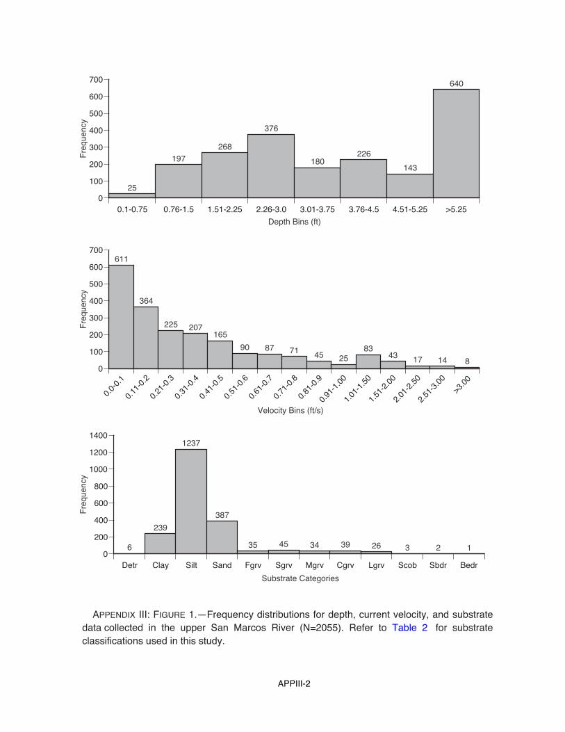
APPIII-2

0.0-

0.1

0.11

-0.2

0.21

-0.3

0.31

-0.4

0.41

-0.5

0.51

-0.6

0.61

-0.7

0.71

-0.8

0.81

-0.9

0.91

-1.0

0

1.01

-1.5

0

1.51

-2.0

0

2.01

-2.5

0

2.51

-3.0

0

>3.0

00

100

200

300

400

500

600

700

Fre

quen

cy

Velocity Bins (ft/s)

611

364

225 207165

90 87 71 45 2583

43 17 14 8

Detr Clay Silt Sand Fgrv Sgrv Mgrv Cgrv Lgrv Scob Sbdr Bedr0

200

400

600

800

1000

1200

1400

Fre

quen

cy

Substrate Categories

6

239

1237

387

35 45 34 39 26 3 2 1

0.1-0.75 0.76-1.5 1.51-2.25 2.26-3.0 3.01-3.75 3.76-4.5 4.51-5.25 >5.250

100

200

300

400

500

600

700F

requ

ency

Depth Bins (ft)

25

197

268

376

180226

143

640

APPENDIX III: FIGURE 1.—Frequency distributions for depth, current velocity, and substratedata collected in the upper San Marcos River (N=2055). Refer to Table 2 for substrateclassifications used in this study.

APPIII-3

APPENDIX III: FIGURE 2.—Suitability criteria for Zizania texana for depth, currentvelocity, and substrate in the upper San Marcos River. Preference indices are indicatedby solid lines or bars (substrate) and supplemental velocity curves are represented bydashed lines. Idealized habitat utilization curves are represented by heavy lines. Refer toTable 2 for substrate classifications used in this study.

Detr Clay Silt Sand Fgrv Sgrv Mgrv Cgrv Lgrv Scob Sbdr Bedr0.00.10.20.30.40.5

0.60.70.80.91.0

Sui

tabi

lity

Substrate Categories

0.0-

0.1

0.11

-0.2

0.21

-0.3

0.31

-0.4

0.41

-0.5

0.51

-0.6

0.61

-0.7

0.71

-0.8

0.81

-0.9

0.91

-1.0

0

1.01

-1.5

0

1.51

-2.0

0

2.01

-2.5

0

2.51

-3.0

0

>3.0

00.00.10.20.3

0.40.50.60.70.80.91.0

Sui

tabi

lity

Velocity Bins (ft/s)

0.1-0.75 0.76-1.5 1.51-2.25 2.26-3.0 3.01-3.75 3.76-4.5 4.51-5.25 >5.250.00.10.2

0.30.40.50.60.70.80.91.0

Sui

tabi

lity

Depth Bins (ft)

APPIII-4

APPENDIX III: FIGURE 3.—Suitability criteria for Heteranthera liebmannii for depth,current velocity, and substrate in the upper San Marcos River. Preference indices areindicated by solid lines or bars (substrate) and supplemental velocity curves arerepresented by dashed lines. Idealized habitat utilization curves are represented by heavylines. Refer to Table 2 for substrate classifications used in this study.

Detr Clay Silt Sand Fgrv Sgrv Mgrv Cgrv Lgrv Scob Sbdr Bedr0.00.10.20.30.40.50.6

0.70.80.91.0

Sui

tabi

lity

Substrate Categories

0.0-

0.1

0.11

-0.2

0.21

-0.3

0.31

-0.4

0.41

-0.5

0.51

-0.6

0.61

-0.7

0.71

-0.8

0.81

-0.9

0.91

-1.0

0

1.01

-1.5

0

1.51

-2.0

0

2.01

-2.5

0

2.51

-3.0

0

>3.0

00.00.10.2

0.30.40.50.60.70.80.91.0

Sui

tabi

lity

Velocity Bins (ft/s)

0.1-0.75 0.76-1.5 1.51-2.25 2.26-3.0 3.01-3.75 3.76-4.5 4.51-5.25 >5.250.00.1

0.20.30.40.50.60.70.80.91.0

Sui

tabi

lity

Depth Bins (ft)

APPIII-5

Detr Clay Silt Sand Fgrv Sgrv Mgrv Cgrv Lgrv Scob Sbdr Bedr0.00.10.20.30.40.50.60.70.80.91.0

Sui

tabi

lity

Substrate Categories

APPENDIX III: FIGURE 4.—Suitability criteria for Vallisneria americana for depth, currentvelocity, and substrate in the upper San Marcos River. Preference indices are indicatedby solid lines or bars (substrate) and supplemental velocity curves are represented bydashed lines. Idealized habitat utilization curves are represented by heavy lines. Refer toTable 2 for substrate classifications used in this study.

0.0-

0.1

0.11

-0.2

0.21

-0.3

0.31

-0.4

0.41

-0.5

0.51

-0.6

0.61

-0.7

0.71

-0.8

0.81

-0.9

0.91

-1.0

0

1.01

-1.5

0

1.51

-2.0

0

2.01

-2.5

0

2.51

-3.0

0

>3.0

00.00.10.20.30.40.50.60.70.80.91.0

Sui

tabi

lity

Velocity Bins (ft/s)

0.1-0.75 0.76-1.5 1.51-2.25 2.26-3.0 3.01-3.75 3.76-4.5 4.51-5.25 >5.250.00.10.20.30.40.50.60.70.80.91.0

Sui

tabi

lity

Depth Bins (ft)

APPIII-6

Detr Clay Silt Sand Fgrv Sgrv Mgrv Cgrv Lgrv Scob Sbdr Bedr0.00.10.20.30.40.50.60.70.80.91.0

Sui

tabi

lity

Substrate Categories

0.1-0.75 0.76-1.5 1.51-2.25 2.26-3.0 3.01-3.75 3.76-4.5 4.51-5.25 >5.250.00.10.20.30.40.50.60.70.80.91.0

Sui

tabi

lity

Depth Bins (ft)

0.0-

0.1

0.11

-0.2

0.21

-0.3

0.31

-0.4

0.41

-0.5

0.51

-0.6

0.61

-0.7

0.71

-0.8

0.81

-0.9

0.91

-1.0

0

1.01

-1.5

0

1.51

-2.0

0

2.01

-2.5

0

2.51

-3.0

0

>3.0

00.00.10.20.30.40.50.60.70.80.91.0

Sui

tabi

lity

Velocity Bins (ft/s)

APPENDIX III: FIGURE 5.—Suitability criteria for Sagittaria platyphylla for depth, currentvelocity, and substrate in the upper San Marcos River. Preference indices are indicatedby solid lines or bars (substrate) and supplemental velocity curves are represented bydashed lines. Idealized habitat utilization curves are represented by heavy lines. Refer toTable 2 for substrate classifications used in this study.

APPIII-7

APPENDIX III: FIGURE 6.—Suitability criteria for Potamogeton illinoensis for depth,current velocity, and substrate in the upper San Marcos River. Preference indices areindicated by solid lines or bars (substrate) and supplemental velocity curves arerepresented by dashed lines. Idealized habitat utilization curves are represented by heavylines. Refer to Table 2 for substrate classifications used in this study.

Detr Clay Silt Sand Fgrv Sgrv Mgrv Cgrv Lgrv Scob Sbdr Bedr0.00.10.20.30.40.50.60.70.80.91.0

Sui

tabi

lity

Substrate Categories

0.0-

0.1

0.11

-0.2

0.21

-0.3

0.31

-0.4

0.41

-0.5

0.51

-0.6

0.61

-0.7

0.71

-0.8

0.81

-0.9

0.91

-1.0

0

1.01

-1.5

0

1.51

-2.0

0

2.01

-2.5

0

2.51

-3.0

0

>3.0

00.00.10.20.30.40.50.60.70.80.91.0

Sui

tabi

lity

Velocity Bins (ft/s)

0.1-0.75 0.76-1.5 1.51-2.25 2.26-3.0 3.01-3.75 3.76-4.5 4.51-5.25 >5.250.00.10.20.30.40.50.60.70.80.91.0

Sui

tabi

lity

Depth Bins (ft)

APPIII-8

APPENDIX III: FIGURE 7.—Suitability criteria for Cabomba caroliniana (n=143) for depth,current velocity, and substrate in the upper San Marcos River. Refer to Table 2 forsubstrate classifications used in this study.

Detr Clay Silt Sand Fgrv Sgrv Mgrv Cgrv Lgrv Scob Sbdr Bedr0.00.10.20.30.40.50.60.70.80.91.0

Sui

tabi

lity

Substrate Categories

0 0

1

0.19

0 0 0 0 0 0 0 0

0.0-

0.1

0.11

-0.2

0.21

-0.3

0.31

-0.4

0.41

-0.5

0.51

-0.6

0.61

-0.7

0.71

-0.8

0.81

-0.9

0.91

-1.0

0

1.01

-1.5

0

1.51

-2.0

0

2.01

-2.5

0

2.51

-3.0

0

>3.0

00.00.10.20.30.40.50.60.70.80.91.0

Sui

tabi

lity

Velocity Bins (ft/s)

1

0.21 0.170.1

0.060 0

0.080.12

0 0 0 0 0 0

0.1-0.75 0.76-1.5 1.51-2.25 2.26-3.0 3.01-3.75 3.76-4.5 4.51-5.25 >5.250.00.10.20.30.40.50.60.70.80.91.0

Sui

tabi

lity

Depth Bins (ft)

1

0.870.94

1

0.89

0.4

0.24

0.75

APPIII-9

APPENDIX III: FIGURE 8.—Suitability criteria for Hydrilla verticillata (n=730) for depth,current velocity, and substrate in the upper San Marcos River. Refer to Table 2 forsubstrate classifications used in this study.

Detr Clay Silt Sand Fgrv Sgrv Mgrv Cgrv Lgrv Scob Sbdr Bedr0.00.10.20.30.40.50.60.70.80.91.0

Sui

tabi

lity

Substrate Categories

00.06

0.67

1

0.26

0.82 0.82

0.62

0.78

0.62

0.93

0

0.0-

0.1

0.11

-0.2

0.21

-0.3

0.31

-0.4

0.41

-0.5

0.51

-0.6

0.61

-0.7

0.71

-0.8

0.81

-0.9

0.91

-1.0

0

1.01

-1.5

0

1.51

-2.0

0

2.01

-2.5

0

2.51

-3.0

0

>3.0

00.00.10.20.30.40.50.60.70.80.91.0

Sui

tabi

lity

Velocity Bins (ft/s)

0.7

0.550.65

0.830.92 0.89

0.94

0.61

0.860.82

0.86

1 0.96

0.15

0

0.1-0.75 0.76-1.5 1.51-2.25 2.26-3.0 3.01-3.75 3.76-4.5 4.51-5.25 >5.250.00.10.20.30.40.50.60.70.80.91.0

Sui

tabi

lity

Depth Bins (ft)

0.46

0.780.84

0.78

1

0.830.73

0.4

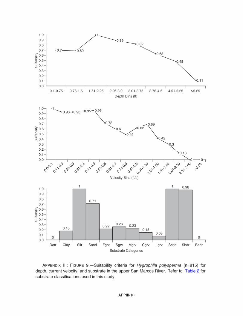
APPIII-10

APPENDIX III: FIGURE 9.—Suitability criteria for Hygrophila polysperma (n=815) fordepth, current velocity, and substrate in the upper San Marcos River. Refer to Table 2 forsubstrate classifications used in this study.

Detr Clay Silt Sand Fgrv Sgrv Mgrv Cgrv Lgrv Scob Sbdr Bedr0.00.10.20.30.40.50.60.70.80.91.0

Sui

tabi

lity

Substrate Categories

0

0.18

1

0.71

0.220.26 0.23

0.150.08

1 0.98

0

0.0-

0.1

0.11

-0.2

0.21

-0.3

0.31

-0.4

0.41

-0.5

0.51

-0.6

0.61

-0.7

0.71

-0.8

0.81

-0.9

0.91

-1.0

0

1.01

-1.5

0

1.51

-2.0

0

2.01

-2.5

0

2.51

-3.0

0

>3.0

00.00.10.20.30.40.50.60.70.80.91.0

Sui

tabi

lity

Velocity Bins (ft/s)

10.93 0.93 0.95 0.96

0.72

0.6

0.49

0.620.69

0.42

0.3

0.13

0 0

0.1-0.75 0.76-1.5 1.51-2.25 2.26-3.0 3.01-3.75 3.76-4.5 4.51-5.25 >5.250.00.10.20.30.40.50.60.70.80.91.0

Sui

tabi

lity

Depth Bins (ft)

0.7 0.69

1

0.890.82

0.63

0.48

0.11

APPIII-11

APPENDIX III: FIGURE 10.—Suitability criteria for Egeria densa (n=289) for depth, currentvelocity, and substrate in the upper San Marcos River. Refer to Table 2 for substrateclassifications used in this study.

Detr Clay Silt Sand Fgrv Sgrv Mgrv Cgrv Lgrv Scob Sbdr Bedr0.00.10.20.30.40.50.60.70.80.91.0

Sui

tabi

lity

Substrate Categories

0 0

1

0.24

0.40.31

0 0 0 0 0 0

0.0-

0.1

0.11

-0.2

0.21

-0.3

0.31

-0.4

0.41

-0.5

0.51

-0.6

0.61

-0.7

0.71

-0.8

0.81

-0.9

0.91

-1.0

0

1.01

-1.5

0

1.51

-2.0

0

2.01

-2.5

0

2.51

-3.0

0

>3.0

00.00.10.20.30.40.50.60.70.80.91.0

Sui

tabi

lity

Velocity Bins (ft/s)

0.911

0.66

0.87

0.57

0.440.34

0

0.11

0.4

0.18

0 0 0 0

0.1-0.75 0.76-1.5 1.51-2.25 2.26-3.0 3.01-3.75 3.76-4.5 4.51-5.25 >5.250.00.10.20.30.40.50.60.70.80.91.0

Sui

tabi

lity

Depth Bins (ft)

0

0.63

0.840.91

0.86

1

0.53

0.21

APPIV-1

Appendix IVInstream Habitat Model Output

APPIV-2

10

12

14

16

18

20

22

24

26

28

30

32

34

36

38

40

42

44

20 30 40 50 60 70 80 90 100 110 120 130 140 150 160 170 180 190 200 210 220

% W

UA

Z. texana

H. liebmannii

V. americana

S. platyphylla

P. illinoensis

Discharge (ft3/s)

APPENDIX IV: FIGURE 1.—Percent weighted usable area (% WUA) in relation to discharge in thenatural channel of the upper San Marcos River for the five target species.

APPIV-3

Segment 1

20

30

40

50

60

70

%W

UA

Segment 2

18

23

28

33

38

%W

UA

Segment 3

32

37

42

47

52%

WU

A

Monthly Hydrograph

050

100150200250300350400450500

1956

1957

1958

1959

1960

1961

1962

1963

1964

1965

1966

1967

1968

1969

1970

1971

1972

1973

1974

1975

1976

1977

1978

1979

1980

1981

1982

1983

1984

1985

1986

1987

1988

1989

1990

1991

1992

1993

1994

1995

1996

1997

1998Mon

thly

ave

rage

spr

ing

flow

(ft3 /s

)

APPENDIX IV: FIGURE 2.—Habitat time series for Zizania texana. Upper horizontal black linesrepresent the 75th percentile % weighted usable area (WUA). Lower horizontal black linesrepresent the 25th percentile %WUA. Horizontal gray line on hydrograph represents monthlymean spring flow based upon the period from 26 May 1956 – 30 September 1998 (USGS Gage#08170000).

APPIV-4

Segment 1

34

39

44

49

54

%W

UA

Segment 2

18

23

28

33

%W

UA

Segment 3

20

25

30

35

40%

WU

A

Monthly Hydrograph

050

100150200250300350400450500

1956

1957

1958

1959

1960

1961

1962

1963

1964

1965

1966

1967

1968

1969

1970

1971

1972

1973

1974

1975

1976

1977

1978

1979

1980

1981

1982

1983

1984

1985

1986

1987

1988

1989

1990

1991

1992

1993

1994

1995

1996

1997

1998

Mon

thly

ave

rage

spr

ing

flow

(ft

3 /s)

APPENDIX IV: FIGURE 3.—Habitat time series for Heteranthera liebmannii. Upperhorizontal black lines represent the 75th percentile % weighted usable area (WUA). Lowerhorizontal black lines represent the 25th percentile %WUA. Horizontal gray line onhydrograph represents monthly mean spring flow based upon the period from 26 May1956 – 30 September 1998 (USGS Gage #08170000).

APPIV-5

Segment 1

10

15

20

25

30

35

40

45

%W

UA

Segment 2

13

15

17

19

21

%W

UA

Segment 3

15

20

25

30

35%

WU

A

Monthly Hydrograph

050

100150200250300350400450500

1956

1957

1958

1959

1960

1961

1962

1963

1964

1965

1966

1967

1968

1969

1970

1971

1972

1973

1974

1975

1976

1977

1978

1979

1980

1981

1982

1983

1984

1985

1986

1987

1988

1989

1990

1991

1992

1993

1994

1995

1996

1997

1998M

onth

ly a

vera

ge s

prin

g flo

w (

ft3 /s)

APPENDIX IV: FIGURE 4.—Habitat time series for Vallisneria americana. Upperhorizontal black lines represent the 75th percentile % weighted usable area (WUA). Lowerhorizontal black lines represent the 25th percentile %WUA. Horizontal gray line onhydrograph represents monthly mean spring flow based upon the period from 26 May1956 – 30 September 1998 (USGS Gage #08170000).

APPIV-6

Segment 1

252627282930313233

%W

UA

Segment 2

323436384042444648

%W

UA

Segment 3

40

45

50

55

%W

UA

Monthly Hydrograph

050

100150200250300350400450500

1956

1957

1958

1959

1960

1961

1962

1963

1964

1965

1966

1967

1968

1969

1970

1971

1972

1973

1974

1975

1976

1977

1978

1979

1980

1981

1982

1983

1984

1985

1986

1987

1988

1989

1990

1991

1992

1993

1994

1995

1996

1997

1998M

onth

ly a

vera

ge s

prin

g flo

w (

ft3 /s

)

APPENDIX IV: FIGURE 5.—Habitat time series for Sagitteria platyphylla. Upperhorizontal black lines represent the 75th percentile % weighted usable area (WUA). Lowerhorizontal black lines represent the 25th percentile %WUA. Horizontal gray line onhydrograph represents monthly mean spring flow based upon the period from 26 May1956 – 30 September 1998 (USGS Gage #08170000).

APPIV-7

Segment 1

44

49

54

59

64

%W

UA

Segment 2

44

46

48

50

52

54

56

%W

UA

Segment 3

44

49

54

59

64

69

74

%W

UA

Monthly Hydrograph

050

100150200250300350400450500

1956

1957

1958

1959

1960

1961

1962

1963

1964

1965

1966

1967

1968

1969

1970

1971

1972

1973

1974

1975

1976

1977

1978

1979

1980

1981

1982

1983

1984

1985

1986

1987

1988

1989

1990

1991

1992

1993

1994

1995

1996

1997

1998M

onth

ly a

vera

ge s

prin

g flo

w (

ft3 /s)

APPENDIX IV: FIGURE 6.—Habitat time series for Potamogeton illinoensis. Upperhorizontal black lines represent the 75th percentile % weighted usable area (WUA). Lowerhorizontal black lines represent the 25th percentile %WUA. Horizontal gray line onhydrograph represents monthly mean spring flow based upon the period from 26 May1956 – 30 September 1998 (USGS Gage #08170000).

APPIV-8

558

559

560

561

562

563

564

565

566

567

568

Ele

vatio

n (m

sl ft

)

558

559

560

561

562

563

564

565

566

567

568

Ele

vatio

n (m

sl ft

)

558

559

560

561

562

563

564

565

566

567

568

0 5 10 15 20 25 30 35 40 45 50 55 60 65 70 75 80 85 90 95

Ele

vatio

n (m

sl ft

)Discharge = 157 ft3/sWSE = 562.66 msl

Depth 1 = 3.41 ft Depth 5 = 2.16 ft

Depth 2 = 3.71 ft Depth 6 = 1.28 ft

Depth 3 = 3.21 ft Depth 7 = 2.66 ft

Depth 4 = 3.21 ft Depth 8 = 2.41 ft

Discharge = 132 ft3/sWSE = 562.45 msl

Discharge = 53 ft3/sWSE = 561.50 msl

Station (ft)

1 2 3 4 5 7 86

1 2 3 4 5 7 8

1 2 3 4 7 8

Depth 1 = 3.20 ft Depth 5 = 1.95 ft

Depth 2 = 3.50 ft Depth 6 = 1.00 ft

Depth 3 = 3.00 ft Depth 7 = 2.45 ft

Depth 4 = 3.00 ft Depth 8 = 2.20 ft

Depth 1 = 2.25 ft Depth 5 = 1.00 ft

Depth 2 = 2.55 ft Depth 6 = 0.05 ft

Depth 3 = 2.05 ft Depth 7 = 1.50 ft

Depth 4 = 2.05 ft Depth 8 = 1.25 ft

Appendix IV: Figure 7.—Depths at Z. texana verticals on cross-section 24,representative of run mesohabitat. Using a depth criteria of 1.0 ft, Z. texana vertical 6(13.4% of Z. texana habitat) was eliminated at 132 ft3/s and verticals 5 and 6 (26.8%)were eliminated at 53 ft3/s.

APPIV-9

0

10

20

30

40

50

60

70

80

90

100

40 50 60 70 80 90 100 110 120 130 140 150 160 170 180 190 200 210 220

% H

abita

t

Discharge (ft3/s)

APPENDIX IV: FIGURE 8.—Percentage of Z. texana habitat meeting depth criterias in relation to dischargein the upper San Marcos River. Data based on all habitat cross-sections in the main channel with Z. texanapresent. Long-term median spring flow based on water years 1956-1998.

Long-term median

spring flow = 157 ft3/s

Depth Criteria > 2.5 ft

Depth Criteria > 1.0 ft

Depth Criteria > 1.5 ft

Depth Criteria > 2.0 ft

APPV-1

Appendix VWater Quality

APPV-2

APPENDIX V: TABLE 1.—San Marcos River, hourly water temperature data, by station and month.

Temperature (°C)

Month Station N Mean Std Dev Minimum Maximum

Nov-94 1 712 21.6 0.48 20.5 22.8Nov-94 2 638 21.2 0.77 19.5 23.1Nov-94 5 712 21.3 0.94 19.0 23.2Dec-94 1 741 21.2 0.54 18.5 22.7Dec-94 2 739 20.5 0.98 14.7 22.7Dec-94 5 744 20.0 1.27 13.6 22.7Jan-95 1 796 21.1 0.52 19.7 22.3Jan-95 2 745 20.5 0.76 18.8 22.3Jan-95 5 739 20.0 0.92 18.1 21.9Feb-95 1 669 21.2 0.52 20.1 22.8Feb-95 2 669 20.7 0.80 19.0 23.0Feb-95 3 538 20.6 0.86 18.6 22.9Feb-95 4 538 20.6 1.11 18.5 23.9Feb-95 5 441 20.0 0.86 18.3 22.1Mar-95 1 692 21.5 0.72 19.7 23.6Mar-95 2 678 21.2 1.14 18.2 24.2Mar-95 3 691 21.1 1.18 18.0 24.1Mar-95 4 203 20.9 0.85 18.6 23.9Mar-95 5 679 21.0 1.33 17.2 24.1Mar-95 6 677 19.9 2.04 15.4 24.3Apr-95 1 720 21.9 0.60 20.0 23.4Apr-95 3 492 21.8 0.96 18.8 23.9Apr-95 4 720 21.9 1.06 18.5 24.4Apr-95 5 720 21.9 1.06 18.5 24.3Apr-95 6 720 21.6 1.36 18.3 24.1May-95 1 712 22.2 0.50 20.9 23.5May-95 2 705 22.5 0.81 20.0 24.4May-95 3 58 22.0 0.64 20.9 23.1May-95 4 202 22.4 0.77 20.1 23.9May-95 5 712 22.9 0.85 20.3 25.2May-95 6 742 24.3 1.11 22.1 27.6Jun-95 1 642 22.3 0.46 21.6 23.3Jun-95 2 516 22.6 0.80 21.3 24.3Jun-95 3 237 22.4 0.79 21.2 23.9Jun-95 4 502 22.9 0.81 21.6 25.0Jun-95 5 642 23.0 0.81 21.5 24.7Jun-95 6 635 25.6 1.02 23.2 28.0Jul-95 1 620 22.5 0.51 21.8 23.6Jul-95 2 409 23.0 0.82 21.9 24.7Jul-95 3 590 22.6 0.82 21.4 24.3Jul-95 4 602 23.5 0.86 22.2 25.3Jul-95 5 612 23.5 0.82 22.1 25.2Jul-95 6 720 26.6 0.67 24.8 28.3Aug-95 1 643 22.6 0.53 21.9 24.3Aug-95 2 744 23.0 0.81 21.8 25.0Aug-95 3 738 23.0 0.82 21.6 25.0Aug-95 4 739 23.3 0.79 22.0 25.0Aug-95 5 644 23.6 0.76 22.4 25.1Aug-95 6 739 26.0 0.77 23.7 28.1Sep-95 1 666 22.4 0.58 21.0 23.8Sep-95 2 655 22.7 0.89 20.2 24.7Sep-95 3 667 22.7 0.89 20.3 24.7Sep-95 4 675 22.8 0.93 20.2 25.6Sep-95 5 596 23.0 1.00 20.2 25.4Sep-95 6 675 24.3 1.22 20.6 26.5Oct-95 1 647 21.8 0.55 19.1 23.3Oct-95 2 681 21.7 0.83 18.6 23.9Oct-95 3 716 21.8 0.85 18.8 24.0Oct-95 4 735 21.7 0.92 18.9 25.1Oct-95 5 689 21.8 0.90 19.2 23.9Oct-95 6 736 22.0 1.00 19.9 26.0Nov-95 1 578 21.4 0.50 19.8 22.4Nov-95 2 581 20.9 0.78 18.6 22.5Nov-95 3 720 20.8 0.81 18.7 22.6Nov-95 4 720 20.5 0.86 18.6 22.5Nov-95 5 581 20.5 0.89 18.2 22.5Nov-95 6 720 19.8 0.90 17.7 21.6Dec-95 1 644 21.0 0.67 19.6 22.8Dec-95 2 646 20.3 1.06 17.9 22.9Dec-95 3 671 20.3 1.13 17.7 24.1

APPV-3

Appendix V: TABLE 1. Continued.—San Marcos River, hourly water temperature data, by station andmonth.

Temperature (°C)

Month Station N Mean Std Dev Minimum Maximum

Dec-95 4 672 19.9 1.19 17.1 22.7Dec-95 5 646 19.7 1.32 16.8 22.6Dec-95 6 670 18.8 1.62 16.1 21.9Dec-95 7 564 18.4 1.55 16.0 21.6Jan-96 1 637 20.7 0.74 19.1 22.4Jan-96 2 688 19.9 1.14 17.2 22.2Jan-96 3 744 19.7 1.12 17.1 22.1Jan-96 4 744 19.4 1.22 16.3 21.8Jan-96 5 694 19.2 1.32 15.9 21.7Jan-96 6 744 18.0 1.45 14.5 21.1Jan-96 7 693 17.9 1.46 14.4 20.6Feb-96 1 571 21.0 1.05 18.8 23.4Feb-96 2 572 20.4 1.64 17.1 23.7Feb-96 3 659 20.3 1.57 16.9 23.5Feb-96 4 663 20.0 1.81 16.0 23.2Feb-96 5 572 19.8 2.02 15.5 23.1Feb-96 6 659 19.2 2.38 14.0 23.2Feb-96 7 573 19.1 2.54 13.9 22.7Mar-96 1 622 21.0 0.95 18.7 23.4Mar-96 2 546 20.5 1.49 16.4 23.8Mar-96 3 768 20.4 1.53 16.3 24.0Mar-96 4 768 20.2 1.63 16.2 23.7Mar-96 5 624 19.9 1.68 16.0 23.2Mar-96 6 768 19.5 1.94 15.4 23.4Mar-96 7 492 19.2 2.06 15.5 22.9Apr-96 1 496 22.2 0.75 20.7 24.1Apr-96 2 497 22.3 1.17 19.7 25.0Apr-96 3 720 21.8 1.47 15.8 24.8Apr-96 4 720 21.8 1.55 15.2 24.9Apr-96 5 497 22.3 1.13 19.4 24.7Apr-96 6 720 22.0 1.68 16.4 25.0Apr-96 7 481 22.6 1.03 19.9 25.0May-96 1 681 22.9 0.65 21.9 24.4May-96 2 681 23.4 1.00 21.7 25.8May-96 3 736 23.4 0.97 21.4 25.5May-96 4 736 23.6 0.95 21.2 25.9May-96 5 681 23.8 0.91 22.1 26.0May-96 6 736 24.5 0.94 21.4 26.9May-96 7 681 24.5 0.86 22.6 26.5Jun-96 1 651 23.2 0.71 21.7 24.7Jun-96 2 603 23.8 1.08 21.5 26.1Jun-96 3 720 23.8 1.03 21.6 26.0Jun-96 4 720 24.2 0.92 22.0 26.1Jun-96 5 650 24.4 0.87 22.0 26.2Jun-96 6 720 25.6 0.80 23.2 27.4Jun-96 7 420 25.4 0.91 23.3 27.3Jul-96 1 650 23.3 0.70 22.3 24.8Jul-96 2 651 24.1 0.97 22.5 26.0Jul-96 3 667 24.1 0.92 22.6 25.9Jul-96 4 667 24.6 0.77 23.0 25.9Jul-96 5 652 25.0 0.66 23.6 26.2Jul-96 6 666 26.3 0.64 25.0 27.9Jul-96 7 547 26.1 0.50 25.0 27.3Aug-96 1 439 23.3 0.75 22.1 24.8Aug-96 3 744 23.8 0.94 22.1 25.9Aug-96 4 744 24.2 0.78 22.7 25.9Aug-96 5 706 24.7 0.78 22.9 26.2Aug-96 6 744 25.6 0.98 23.2 27.6Aug-96 7 706 25.5 0.87 23.5 27.3Sep-96 1 584 22.6 0.64 21.0 24.1Sep-96 2 584 22.9 1.01 20.0 24.9Sep-96 3 82 23.2 0.87 22.1 25.0Sep-96 4 720 23.2 0.96 20.0 25.1Sep-96 5 665 23.4 1.02 20.0 25.4Sep-96 6 719 24.2 1.01 20.4 25.6Sep-96 7 652 24.0 1.00 20.4 25.4Oct-96 1 608 22.1 0.59 20.5 23.6Oct-96 2 324 22.1 0.90 20.1 24.1Oct-96 3 542 21.9 0.96 19.2 24.0

APPV-4

Appendix V: TABLE 1. Continued.—San Marcos River, hourly water temperature data, by station andmonth.

Temperature (°C)

Month Station N Mean Std Dev Minimum Maximum

Oct-96 4 744 22.0 0.96 19.1 24.0Oct-96 5 607 22.1 1.01 19.1 24.1Oct-96 6 745 22.3 1.04 19.1 24.3Oct-96 7 563 22.2 1.14 19.0 24.4Nov-96 1 645 21.2 0.77 19.3 22.8Nov-96 2 561 20.6 1.27 16.7 22.7Nov-96 3 719 20.6 1.29 16.4 22.9Nov-96 4 720 20.4 1.43 16.3 23.2Nov-96 5 647 20.3 1.47 16.4 23.2Nov-96 6 719 20.1 1.75 15.8 23.1Nov-96 7 647 19.9 1.80 15.6 23.1Dec-96 1 641 20.7 0.91 18.6 22.6Dec-96 2 642 20.0 1.40 15.9 22.4Dec-96 3 744 19.8 1.36 15.8 22.3Dec-96 4 743 19.4 1.53 15.4 22.0Dec-96 5 642 19.3 1.69 15.5 21.9Dec-96 6 744 18.4 1.83 14.2 21.6Dec-96 7 643 18.2 1.96 14.0 21.2Jan-97 1 538 20.4 1.03 18.4 22.5Jan-97 2 527 19.4 1.55 16.6 22.3Jan-97 3 744 19.3 1.61 16.3 22.8Jan-97 4 744 18.9 1.80 15.4 22.7Jan-97 5 540 18.5 1.88 14.9 21.7Jan-97 6 744 17.5 2.39 12.8 21.9Jan-97 7 541 17.0 2.33 12.6 20.9Feb-97 1 537 20.7 0.63 18.3 22.3Feb-97 2 537 19.8 1.08 16.0 22.2Feb-97 3 672 19.8 1.15 16.1 22.6Feb-97 4 672 19.5 1.29 15.1 22.3Feb-97 5 420 19.0 1.34 15.1 21.4Feb-97 6 672 18.3 1.54 14.5 21.9Feb-97 7 537 17.2 1.21 14.4 20.6Mar-97 1 679 21.7 0.63 20.3 23.5Mar-97 2 676 21.4 1.03 19.2 24.3Mar-97 3 729 21.2 1.02 19.0 24.1Mar-97 4 733 21.2 1.06 18.9 24.0Mar-97 5 12 20.7 0.29 20.2 21.0Mar-97 6 729 21.1 1.42 18.5 24.1Mar-97 7 679 19.9 1.27 17.4 22.5Apr-97 1 705 21.7 0.60 18.8 23.5Apr-97 2 705 21.5 1.05 17.4 24.4Apr-97 7 705 19.6 1.67 16.3 23.6May-97 1 32 22.2 0.46 21.6 23.1May-97 2 33 22.2 0.70 21.5 23.7May-97 7 110 22.6 0.94 19.9 24.0

APPV-5

APPENDIX V: TABLE 2.—San Marcos River, dissolved oxygen by station and month. All data are from thefirst four days following data sonde calibration.

Dissolved Oxygen (mg/L)

Month Station N Mean Std Dev Minimum Maximum

Nov-94 1 96 6.3 0.61 5.4 7.7Nov-94 2 96 7.4 0.81 6.3 9.1Nov-94 5 96 5.3 0.34 4.6 6.2Feb-95 1 96 7.5 0.73 6.6 9.0Feb-95 2 96 7.7 1.28 6.2 10.4Feb-95 5 96 7.1 0.78 6.0 9.1Mar-95 1 96 7.0 0.68 6.1 8.6Mar-95 2 96 8.1 1.19 6.9 10.9Mar-95 5 96 7.3 0.71 6.2 8.9Apr-95 1 96 7.5 0.79 6.7 9.8Apr-95 5 96 6.9 0.63 5.8 8.9May-95 1 96 8.5 1.09 7.2 10.6May-95 2 96 6.9 1.22 5.4 9.8May-95 5 96 6.2 0.55 5.2 7.4Jun-95 1 96 7.6 0.81 6.6 8.9Jun-95 2 96 7.7 1.08 6.3 9.7Jun-95 5 96 8.2 0.49 7.6 9.3Jul-95 1 96 7.8 0.85 6.7 9.3Jul-95 2 96 7.9 1.41 6.3 10.5Jul-95 5 96 8.7 0.64 8.0 9.9Aug-95 1 96 7.5 0.76 6.7 9.0Aug-95 2 96 5.5 1.22 4.2 8.5Aug-95 5 96 7.7 0.53 7.0 8.9Sep-95 1 96 7.4 0.82 6.4 9.2Sep-95 2 96 7.2 1.35 5.6 10.2Sep-95 5 96 7.7 0.70 6.8 9.2Oct-95 1 96 8.2 0.87 7.3 9.7Oct-95 2 95 8.0 1.07 7.0 10.2Oct-95 5 96 7.4 0.46 6.8 8.3Nov-95 1 95 7.5 0.68 6.7 9.0Nov-95 2 96 7.4 0.87 6.3 9.3Nov-95 5 96 7.2 0.46 6.0 8.1Dec-95 1 96 8.1 0.71 7.3 9.6Dec-95 2 96 8.1 1.22 6.7 10.8Dec-95 5 96 8.1 0.69 7.2 9.6Dec-95 7 96 9.3 0.27 8.8 9.8Jan-96 1 96 8.1 0.66 7.3 9.4Jan-96 2 96 8.3 1.12 6.9 10.7Jan-96 5 96 8.6 0.76 7.7 10.1Jan-96 7 96 9.8 0.25 9.2 10.3Feb-96 1 96 8.4 1.00 7.3 10.2Feb-96 2 96 8.8 1.76 6.8 12.2Feb-96 5 96 8.4 1.24 7.0 10.8Feb-96 7 96 9.4 0.34 8.7 10.0Mar-96 1 96 7.9 1.00 6.2 9.6Mar-96 2 96 6.9 1.45 4.7 10.4Mar-96 5 96 8.1 1.26 6.4 10.4Mar-96 7 96 8.9 0.34 8.3 9.6Apr-96 1 96 8.5 1.20 7.1 10.5Apr-96 2 96 6.5 1.58 4.1 9.9Apr-96 5 96 7.1 1.02 5.6 9.3Apr-96 7 96 7.6 0.36 6.7 8.4May-96 1 96 7.6 1.04 6.4 10.0May-96 2 96 7.6 1.33 5.3 11.1May-96 5 96 6.7 0.76 5.8 8.7May-96 7 96 7.2 0.53 6.1 8.2Jun-96 1 96 8.0 1.18 6.6 9.9Jun-96 2 96 5.7 1.13 3.2 8.4Jun-96 5 96 6.4 0.60 5.5 7.7Jun-96 7 96 7.6 0.32 6.6 8.2Jul-96 1 95 8.2 1.17 6.8 10.1Jul-96 2 96 7.5 1.68 5.1 10.7Jul-96 5 96 6.4 0.71 5.2 7.9Jul-96 7 96 6.9 1.06 5.1 8.6Aug-96 1 96 8.1 1.12 6.7 10.0Aug-96 5 96 7.8 1.39 5.5 10.6Aug-96 7 96 6.3 0.97 5.1 8.7Sep-96 1 96 7.6 0.91 6.6 9.3Sep-96 2 96 7.0 0.93 5.7 9.0

APPV-6

APPENDIX V: TABLE 2. Continued. —San Marcos River, dissolved oxygen by station and month. All data arefrom the first four days following data sonde calibration.

Dissolved Oxygen (mg/L)

Month Station N Mean Std Dev Minimum Maximum

Sep-96 5 96 8.8 0.73 7.5 10.3Sep-96 7 96 7.5 0.20 6.9 7.9Oct-96 1 96 7.8 0.92 6.7 9.5Oct-96 2 96 7.3 1.53 5.6 10.6Oct-96 5 96 6.2 0.85 4.8 8.2Oct-96 7 37 6.6 0.42 5.7 7.3Nov-96 1 96 7.8 0.80 6.9 9.4Nov-96 2 96 6.9 1.00 5.5 8.9Nov-96 5 96 8.2 0.50 7.5 9.2Nov-96 7 96 7.6 0.38 6.6 8.4Dec-96 1 96 7.7 0.79 6.7 9.2Dec-96 2 96 8.1 1.17 6.4 10.5Dec-96 5 96 7.7 0.61 6.7 9.0Dec-96 7 96 8.0 0.40 7.2 8.8Jan-97 1 96 6.5 0.43 5.6 7.6Jan-97 2 96 8.5 0.80 7.4 10.8Jan-97 5 96 7.8 0.50 6.7 8.9Jan-97 7 96 9.6 0.30 8.8 10.1Feb-97 1 96 7.6 0.65 6.8 9.0Feb-97 2 96 7.8 1.12 6.5 10.4Feb-97 5 96 8.7 0.91 6.9 10.8Feb-97 7 96 8.7 0.29 8.0 9.4Mar-97 1 96 7.4 0.58 6.4 8.9Mar-97 7 96 8.3 0.22 7.8 8.8Apr-97 1 96 7.4 0.51 6.2 8.8Apr-97 7 96 9.0 0.80 7.0 10.5

APPV-7

APPENDIX V: TABLE 3.—San Marcos River, pH by station and month.

pH (standard units)

Month Station N Mean Std Dev Minimum Maximum

Nov-94 1 712 7.5 0.07 7.4 7.7Nov-94 2 638 7.7 0.12 7.5 8.1Nov-94 5 712 7.8 0.06 7.7 8.0Dec-94 1 741 7.5 0.06 7.3 7.6Dec-94 2 739 7.8 0.15 7.4 8.1Dec-94 5 744 7.8 0.08 7.6 8.0Jan-95 1 796 7.5 0.08 7.4 7.8Jan-95 2 745 7.8 0.13 7.6 8.2Jan-95 5 739 7.8 0.09 7.6 8.1Feb-95 1 669 7.3 0.07 7.2 7.6Feb-95 2 669 7.7 0.11 7.5 8.0Feb-95 5 441 7.6 0.09 7.5 8.0Mar-95 1 692 7.5 0.07 7.3 7.7Mar-95 2 678 7.6 0.12 7.3 7.9Mar-95 5 678 7.8 0.09 7.6 8.0Apr-95 1 720 7.4 0.07 7.3 7.6Apr-95 5 720 7.6 0.10 7.4 7.9May-95 1 712 7.5 0.08 7.3 7.7May-95 2 705 8.0 0.16 7.7 8.4May-95 5 712 7.8 0.09 7.6 8.1Jun-95 1 642 7.4 0.08 7.3 7.6Jun-95 2 516 7.7 0.25 7.4 8.3Jun-95 5 642 7.7 0.10 7.5 8.0Jul-95 1 620 7.5 0.06 7.4 7.6Jul-95 2 409 7.7 0.10 7.5 7.9Jul-95 5 612 7.8 0.08 7.7 8.2Aug-95 1 643 7.6 0.07 7.5 7.8Aug-95 2 744 7.8 0.13 7.6 8.2Aug-95 5 644 7.9 0.08 7.7 8.1Sep-95 1 666 7.5 0.14 7.3 7.8Sep-95 2 655 7.7 0.18 7.4 8.2Sep-95 5 596 7.9 0.10 7.6 8.2Oct-95 1 647 7.5 0.11 7.2 7.7Oct-95 2 682 7.7 0.09 7.6 8.0Oct-95 5 689 8.0 0.08 7.8 8.2Nov-95 1 578 7.6 0.06 7.4 7.7Nov-95 2 581 7.8 0.09 7.6 8.0Nov-95 5 581 8.0 0.08 7.8 8.2Dec-95 1 644 7.5 0.08 7.4 7.7Dec-95 2 646 7.7 0.11 7.5 8.0Dec-95 5 646 7.9 0.11 7.7 8.2Dec-95 7 564 8.0 0.05 7.9 8.1Jan-96 1 637 7.5 0.07 7.4 7.7Jan-96 2 688 7.7 0.11 7.5 8.0Jan-96 5 694 7.9 0.09 7.7 8.1Jan-96 7 693 8.1 0.04 8.0 8.2Feb-96 1 571 7.6 0.07 7.5 7.9Feb-96 2 572 7.8 0.12 7.5 8.1Feb-96 5 572 8.0 0.09 7.8 8.2Feb-96 7 572 8.2 0.07 8.0 8.3Mar-96 1 622 7.6 0.10 7.4 7.8Mar-96 2 546 7.7 0.14 7.5 8.1Mar-96 5 624 7.9 0.09 7.7 8.2Mar-96 7 492 8.1 0.13 7.9 8.4Apr-96 1 496 7.5 0.08 7.3 7.7Apr-96 2 497 7.5 0.13 7.3 7.8Apr-96 5 497 8.0 0.08 7.8 8.2Apr-96 7 481 8.1 0.07 7.9 8.2May-96 1 681 7.5 0.09 7.3 7.7May-96 2 681 7.8 0.11 7.5 8.0May-96 5 681 8.0 0.11 7.7 8.2May-96 7 681 8.0 0.07 7.8 8.1Jun-96 1 651 7.6 0.08 7.4 7.7Jun-96 2 603 7.8 0.11 7.5 8.1Jun-96 5 650 8.0 0.09 7.7 8.2Jun-96 7 420 8.1 0.09 7.9 8.3Jul-96 1 650 7.5 0.09 7.3 7.7Jul-96 2 651 7.7 0.11 7.5 8.0Jul-96 5 652 7.8 0.06 7.7 8.2Jul-96 7 535 8.0 0.08 7.9 8.2

APPV-8

APPENDIX V: TABLE 3. Continued. —San Marcos River, pH by station and month.

pH (standard units)

Month Station N Mean Std Dev Minimum Maximum

Aug-96 1 429 7.5 0.07 7.4 7.7Aug-96 5 706 7.7 0.07 7.4 8.0Aug-96 7 706 7.9 0.07 7.6 8.0Sep-96 1 584 7.7 0.11 7.4 7.9Sep-96 2 584 7.8 0.14 7.5 8.2Sep-96 5 665 7.9 0.08 7.7 8.1Sep-96 7 652 8.1 0.09 7.9 8.3Oct-96 1 608 7.6 0.14 7.4 8.0Oct-96 2 324 7.8 0.22 7.5 8.3Oct-96 5 607 7.8 0.12 7.6 8.1Oct-96 7 563 8.0 0.20 7.8 8.4Nov-96 1 645 7.6 0.12 7.4 7.9Nov-96 2 561 8.0 0.16 7.7 8.4Nov-96 5 86 7.9 0.05 7.8 7.9Nov-96 7 647 8.1 0.09 7.9 8.3Dec-96 1 641 7.6 0.09 7.4 7.9Dec-96 2 642 7.8 0.15 7.6 8.4Dec-96 7 643 8.0 0.11 7.8 8.4Jan-97 1 538 7.6 0.07 7.5 7.9Jan-97 2 527 8.0 0.13 7.7 8.3Jan-97 5 502 8.1 0.08 7.9 8.4Jan-97 7 541 8.2 0.07 8.0 8.4Feb-97 1 537 7.4 0.06 7.3 7.6Feb-97 2 537 7.7 0.11 7.5 8.0Feb-97 5 420 7.8 0.07 7.7 8.0Feb-97 7 537 7.9 0.06 7.8 8.1Mar-97 1 679 7.5 0.06 7.4 7.7Mar-97 2 676 7.8 0.13 7.6 8.2Mar-97 7 679 8.1 0.10 7.9 8.4Apr-97 1 705 7.5 0.10 7.3 7.7Apr-97 2 705 7.7 0.13 7.4 8.0Apr-97 7 705 8.1 0.14 7.7 8.4May-97 1 32 7.6 0.05 7.5 7.7May-97 2 33 7.7 0.09 7.7 7.9May-97 7 24 8.3 0.02 8.3 8.3

APPV-9

APPENDIX V: TABLE 4.—San Marcos River, specific conductance by station and month.

Specific Conductance (µS/cm)

Month Station N Mean Std Dev Minimum Maximum

Nov-94 1 712 618 6.9 511 637Nov-94 2 638 591 12.1 415 599Nov-94 5 712 629 16.7 451 653Dec-94 1 741 595 9.5 542 637Dec-94 2 739 576 28.7 352 596Dec-94 5 744 595 41.4 355 637Jan-95 1 796 556 38.2 323 608Jan-95 2 745 585 2.4 573 590Jan-95 5 739 599 5.3 532 612Feb-95 1 669 597 11.0 537 604Feb-95 2 669 597 13.1 473 619Feb-95 5 441 618 6.4 569 629Mar-95 1 692 612 6.5 507 618Mar-95 2 678 619 22.4 340 628Mar-95 5 678 565 30.6 255 622Apr-95 1 720 599 6.9 493 608Apr-95 5 720 613 28.9 341 635May-95 1 712 620 13.6 385 629May-95 2 705 624 44.6 182 640May-95 5 712 633 53.5 230 665Jun-95 1 642 604 6.1 555 620Jun-95 2 516 603 20.9 457 641Jun-95 5 642 600 18.1 454 641Jul-95 1 620 589 7.6 536 602Jul-95 2 409 587 4.5 567 592Jul-95 5 612 596 8.7 506 609Aug-95 1 643 584 9.6 385 590Aug-95 2 731 578 20.6 281 585Aug-95 5 643 591 20.2 336 606Sep-95 1 666 618 23.9 290 633Sep-95 2 655 614 40.5 170 633Sep-95 5 596 598 46.8 169 625Oct-95 1 647 591 12.2 335 629Oct-95 2 682 592 22.7 291 630Oct-95 5 689 609 18.9 356 640Nov-95 1 578 592 10.6 365 596Nov-95 2 581 587 30.3 213 599Nov-95 5 581 601 38.5 244 638Dec-95 1 644 609 6.2 592 615Dec-95 2 646 587 4.0 552 593Dec-95 5 646 597 7.3 562 621Dec-95 7 564 629 5.2 607 644Jan-96 1 636 604 2.1 582 608Jan-96 2 688 599 4.2 582 604Jan-96 5 694 609 6.4 590 624Jan-96 7 693 624 5.1 612 636Feb-96 1 571 599 2.4 572 603Feb-96 2 572 586 5.6 574 598Feb-96 5 572 609 5.7 594 627Feb-96 7 572 608 9.6 593 634Mar-96 1 622 612 8.1 558 619Mar-96 2 546 591 10.5 503 603Mar-96 5 624 610 10.1 543 632Mar-96 7 492 605 10.3 553 624Apr-96 1 496 591 6.8 503 598Apr-96 2 497 603 18.2 391 612Apr-96 5 497 594 19.5 397 613Apr-96 7 481 611 18.0 484 629May-96 1 681 595 4.4 499 599May-96 2 681 599 9.4 543 612May-96 5 680 603 9.8 545 626May-96 7 681 589 7.0 558 605Jun-96 1 651 553 21.5 339 596Jun-96 2 603 551 36.2 242 609Jun-96 5 649 590 35.6 299 623Jun-96 7 420 582 43.5 364 603Jul-96 1 650 587 12.6 470 595Jul-96 2 651 589 4.4 557 594Jul-96 5 652 632 10.9 572 653Jul-96 7 535 609 5.3 591 621

APPV-10

APPENDIX V: TABLE 4. Continued.—San Marcos River, specific conductance by station and month.

Specific Conductance (µS/cm)

Month Station N Mean Std Dev Minimum Maximum

Aug-96 1 429 596 15.3 335 603Aug-96 5 706 588 82.7 165 664Aug-96 7 706 567 91.5 203 622Sep-96 1 584 585 10.8 498 593Sep-96 2 584 583 21.9 407 593Sep-96 5 665 601 28.1 436 632Sep-96 7 652 590 27.2 472 615Oct-96 1 608 591 10.4 515 598Oct-96 2 324 588 4.7 552 593Oct-96 5 607 611 8.7 569 632Oct-96 7 563 604 5.9 577 616Nov-96 1 645 591 8.3 513 596Nov-96 2 561 597 23.2 370 605Nov-96 5 647 607 25.8 409 632Nov-96 7 647 600 26.2 430 621Dec-96 1 641 595 7.2 515 600Dec-96 2 642 594 23.1 350 603Dec-96 5 641 608 27.8 371 641Dec-96 7 643 591 27.3 400 614Jan-97 1 538 585 4.0 573 597Jan-97 2 527 596 7.8 432 605Jan-97 5 540 612 6.7 596 630Jan-97 7 541 600 4.2 590 611Feb-97 1 537 583 18.0 430 595Feb-97 2 537 589 22.4 402 605Feb-97 5 420 609 32.0 431 633Feb-97 7 537 573 28.7 455 615Mar-97 1 679 597 7.9 511 605Mar-97 2 676 605 7.1 550 611Mar-97 7 679 563 10.4 535 590Apr-97 1 705 598 13.6 356 605Apr-97 2 705 593 42.2 238 614Apr-97 7 705 499 55.3 273 575May-97 1 32 601 1.2 599 603May-97 2 33 609 1.0 607 611May-97 7 34 523 3.1 518 528

APPV-11

APPENDIX V: TABLE 5.—San Marcos River turbidity measured at water qualitystations 1, 2, 5, and 7. Results are in nephelometric turbidity units (NTU).

Station

Date 1 2 5 7

11/15/94 1.95 1.56 3.57 —12/01/94 1.13 0.97 3.48 —12/15/94 1.86 3.37 6.04 —01/03/95 0.42 0.98 4.30 —01/18/95 0.75 1.04 3.73 —02/03/95 0.44 1.25 2.86 —02/15/95 0.54 1.41 5.05 —03/01/95 1.15 0.85 1.91 —03/15/95 0.66 1.61 3.27 —03/31/95 0.63 1.63 1.93 —04/19/95 0.60 2.11 5.98 —05/01/95 0.75 1.70 5.03 —05/16/95 0.83 1.20 6.64 —06/05/95 0.56 1.54 8.14 —06/21/95 0.64 1.31 5.01 —07/06/95 0.81 1.44 6.98 —08/08/95 0.58 0.86 3.69 —08/17/95 0.36 0.51 3.12 —09/06/95 0.31 0.62 1.63 —09/21/95 5.75 6.13 12.3 —10/03/95 0.71 1.28 3.92 —10/16/95 0.95 1.55 4.81 —11/02/95 1.71 2.38 3.23 —11/15/95 1.51 1.47 4.37 —12/04/95 0.83 1.38 2.68 —12/18/95 1.21 1.60 3.88 —01/03/96 0.51 0.82 1.68 6.4801/16/96 0.57 0.70 1.12 1.5202/05/96 0.47 0.70 1.12 2.6302/09/96 1.09 1.78 2.53 7.1003/04/96 1.66 1.76 4.88 10.603/21/96 0.83 1.97 2.90 9.9703/29/96 1.35 1.54 1.96 2.3404/15/96 0.61 1.80 3.71 7.4004/30/96 0.57 1.47 2.20 4.3605/13/96 0.82 1.86 4.63 9.4606/03/96 2.95 3.51 8.98 9.7806/19/96 1.62 2.55 4.63 7.1107/01/96 1.04 1.23 6.53 8.0407/15/96 1.26 2.38 5.28 13.407/31/96 2.34 5.23 3.00 4.6708/16/96 1.75 1.80 1.30 0.8209/04/96 2.62 3.12 5.02 6.2010/09/96 1.59 3.11 2.73 4.7510/17/96 1.13 1.80 4.73 6.3611/04/96 2.26 2.36 3.02 3.1611/07/96 1.46 1.78 4.69 4.9712/02/96 1.30 2.24 2.56 2.4312/17/96 1.23 1.61 — 8.7301/02/97 1.17 1.08 1.51 2.6401/16/97 2.02 0.50 0.47 0.7701/31/97 0.42 0.90 1.50 0.5702/18/97 1.51 1.32 2.68 3.8203/04/97 0.97 0.90 1.48 3.0003/21/97 0.26 0.61 1.08 1.6403/31/97 1.13 1.49 4.01 7.7604/15/97 1.03 2.06 7.36 12.605/02/97 0.48 0.73 0.40 1.19

N 58 58 57 32Mean 1.17 1.70 3.81 5.51Std Dev 0.86 1.03 2.24 3.58Minimum 0.26 0.50 0.40 0.57Maximum 5.75 6.13 12.3 13.4

APPV-12

15

16

17

18

19

20

21

22

23

24

25

26

27

28

29

JAN FEB MAR APR MAY JUN JUL AUG SEP OCT NOV DEC

Month

Tem

pera

ture

(°C

)

1995 Observed

1995 Predicted

1996 Observed

1996 Predicted

Median Predicted

Minimum Predicted

APPENDIX V: FIGURE 1.—Observed and predicted temperature for water quality station 3:temperature sonde 1 assuming normal air temperature. Bars represent maximum daily temperaturefor the minimum flow scenario.

15

16

17

18

19

20

21

22

23

24

25

26

27

28

29

JAN FEB MAR APR MAY JUN JUL AUG SEP OCT NOV DEC

Month

Tem

pera

ture

(°C

)

1995 Observed

1995 Predicted

1996 Observed

1996 Predicted

Median Predicted

Minimum Predicted

APPENDIX V: FIGURE 2.—Observed and predicted temperature for water quality station 4:temperature sonde 2 assuming normal air temperature. Bars represent maximum daily temperaturefor the minimum flow scenario.

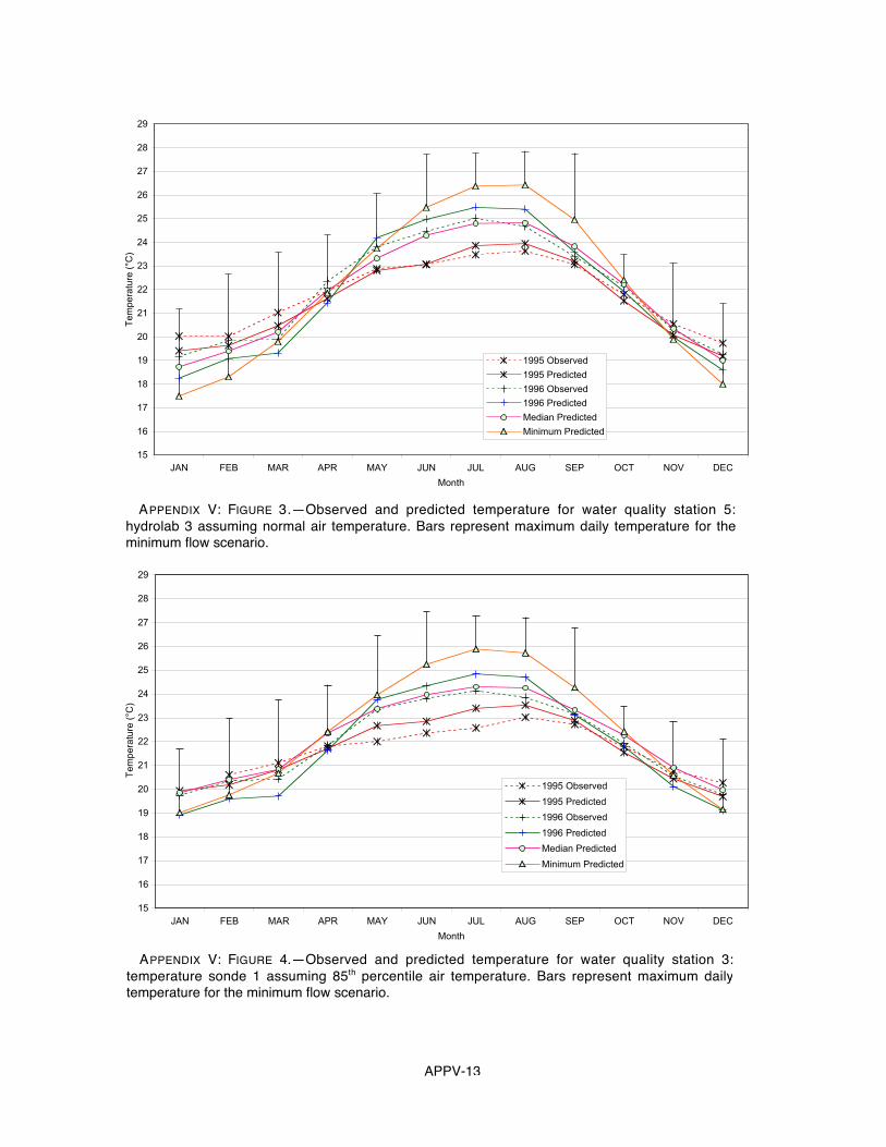
APPV-13

15

16

17

18

19

20

21

22

23

24

25

26

27

28

29

JAN FEB MAR APR MAY JUN JUL AUG SEP OCT NOV DEC

Month

Tem

pera

ture

(°C

)

1995 Observed

1995 Predicted

1996 Observed

1996 Predicted

Median Predicted

Minimum Predicted

APPENDIX V: FIGURE 3.—Observed and predicted temperature for water quality station 5:hydrolab 3 assuming normal air temperature. Bars represent maximum daily temperature for theminimum flow scenario.

15

16

17

18

19

20

21

22

23

24

25

26

27

28

29

JAN FEB MAR APR MAY JUN JUL AUG SEP OCT NOV DEC

Month

Tem

pera

ture

(°C

)

1995 Observed

1995 Predicted

1996 Observed

1996 Predicted

Median Predicted

Minimum Predicted

APPENDIX V: FIGURE 4.—Observed and predicted temperature for water quality station 3:temperature sonde 1 assuming 85th percentile air temperature. Bars represent maximum dailytemperature for the minimum flow scenario.

APPV-14

15

16

17

18

19

20

21

22

23

24

25

26

27

28

29

JAN FEB MAR APR MAY JUN JUL AUG SEP OCT NOV DEC

Month

Tem

pera

ture

(°C

)

1995 Observed

1995 Predicted

1996 Observed

1996 Predicted

Median Predicted

Minimum Predicted

APPENDIX V: FIGURE 5.—Observed and predicted temperature for water quality station 4:temperature sonde 2 assuming 85th percentile air temperature. Bars represent maximum dailytemperature for the minimum flow scenario.

15

16

17

18

19

20

21

22

23

24

25

26

27

28

29

JAN FEB MAR APR MAY JUN JUL AUG SEP OCT NOV DEC

Month

Tem

pera

ture

(°C

)

1995 Observed

1995 Predicted

1996 Observed

1996 Predicted

Median Predicted

Minimum Predicted

APPENDIX V: FIGURE 6.—Observed and predicted temperature for water quality station 5: hydrolab3 assuming 85th percentile air temperature. Bars represent maximum daily temperature for theminimum flow scenario.

APPV-15

23.0

23.5

24.0

24.5

25.0

25.5

26.0

26.5

27.0

27.5

28.0

28.5

29.0

50 60 70 80 90 100 110 120 130 140 150 160 170 180 190 200 250 300 350 400 450

Spring flow (ft3/s)

Wat

er t

emp

erat

ure

(°C

)

Station 3

Station 4

Station 5

Average Temperature

23.0

23.5

24.0

24.5

25.0

25.5

26.0

26.5

27.0

27.5

28.0

28.5

29.0

50 60 70 80 90 100 110 120 130 140 150 160 170 180 190 200 250 300 350 400 450

Spring flow (ft3/s)

Wat

er t

emp

erat

ure

(°C

)

Station 3

Station 4

Station 5

Maximum Temperature

APPENDIX V: FIGURE 7.—Average (upper) and maximum (lower) daily temperaturesmodeled at water quality stations 3, 4 and 5 for a flow range of 50 to 450 ft3/s.Horizontal bars represent temperature criteria. Average temperature criteria equals25°C and maximum temperature criteria equals 26.7°C.