Clark UniversityClark Digital CommonsInternational Development, Community andEnvironment (IDCE) Master’s Papers

4-2019

An Evaluation of Sentinel-1 and Sentinel-2 forLand Cover ClassificationAaron MeneghiniClark University, ameneghini@clarku.edu

Follow this and additional works at: https://commons.clarku.edu/idce_masters_papers

Part of the Geographic Information Sciences Commons, Physical and Environmental GeographyCommons, and the Remote Sensing Commons

This Research Paper is brought to you for free and open access by the Master’s Papers at Clark Digital Commons. It has been accepted for inclusion inInternational Development, Community and Environment (IDCE) by an authorized administrator of Clark Digital Commons. For more information,please contact mkrikonis@clarku.edu, jodolan@clarku.edu.

Recommended CitationMeneghini, Aaron, "An Evaluation of Sentinel-1 and Sentinel-2 for Land Cover Classification" (2019). International Development,Community and Environment (IDCE). 235.https://commons.clarku.edu/idce_masters_papers/235

i

An Evaluation of Sentinel-1 and Sentinel-2 for Land Cover

Classification.

Author: Aaron Meneghini1

1Department of International Development, Community, and Environment. Clark University 950 Main

Street, Worcester, MA. 01610. United States of America.

Date of Degree Conferment: May, 2019

A Master’s Paper

Submitted to the faculty of Clark University, Worcester, Massachusetts, in partial fulfillment of the

requirements for the degree of Master of Sciences in the department of International Development,

Community, and the Environment.

And accepted on the recommendation of

Dr. Florencia Sangermano, Chief Instructor

Signature: _____________________________

ii

Abstract: An Evaluation of Sentinel-1 and Sentinel-2 for Land Cover Classification.

Aaron Meneghini

This study evaluates Sentinel-1 and Sentinel-2 remotely sensed images for tropical land cover

classification. The dual polarized Sentinel-1 VV and VH backscatter images and four 10-meter

multispectral bands of Sentinel-2 were used to create six land cover classification images across two

study areas along the border of the Bolivian Pando Department and the Brazilian state of Acre. Results

indicate that Sentinel-2 multispectral bands possess a higher overall performance in delineating land

cover types than the Sentinel-1 backscatter bands. Sentinel-1 backscatter bands delineated land cover

types based on their surficial properties but did not facilitate the separation of similarly textured classes.

The combination of Sentinel-1 and -2 resulted in higher accuracy for delineating land cover through

increasing the accuracy in delineating the classes of secondary vegetation from exposed soil. While

Sentinel-2 demonstrated the capability to consistently capture land cover in both case studies, there is

potential for single date Sentinel-1 backscatter image to act as ancillary information in Sentinel-2 scenes

affected by clouds or for increasing separability across classes of mixed multispectral qualities but

distinct surficial roughness, such as bare ground versus sparsely vegetation areas.

Dr. Florencia Sangermano, Chief Instructor

iii

ACADEMIC HISTORY

Name: Aaron Meneghini Date: May 2019

Baccalaureate Degree: B.S. Environmental Science

Source: University of Massachusetts, Lowell Date: May 2017

Occupation and Academic Connection since date of baccalaureate degree:

Clark University, M.S. in Geographic Information Science for Development and the Environment

iv

Acknowledgements

I wish to thank my research advisor, Professor Florencia Sangermano, whose support, guidance, and

encouragement enabled me to pursue this project. I am profoundly grateful for her expertise and

patience and I consider it a privilege to have had the opportunity to work with her. I am also grateful to

my family and friends, for their unwavering support throughout my academic career.

v

Table of Contents

List of Illustrations

Tables vi

Figures vii

Introduction 1

Roles of Remote Sensing 2

Background of Synthetic Aperture Radar 2

Copernicus Program 4

Sentinel-2 5

Sentinel-1 7

Combing Sentinel-1 and -2 10

Research Goals 11

Methods 12

Results 17

Discussion 21

Conclusion 25

Figures 26

Literature Cited 44

Appendixes 47

vi

List of Illustrations

Tables:

Table 1. Sensor Specifications for Sentinel-1 and Sentinel-2 26

Table 2. Data Products 26

Table 3. Case 1 Summary Table of Accuracy Assessment 43

Table 4. Case 2 Summary Table of Accuracy Assessment 44

Table 5. Confusion Matrices for Case Study 1 44

Table 6. Confusion Matrices Case Study 2 45

Table 8. Cross Tabulation Matrices, Case Study 1 46

Table 9. Cross Tabulation Matrices, Case Study 2 47

vii

List of Illustrations

Figures:

Figure 1. Study Area Map 27

Figure 2. Case Study 1 and 2 False Color Composites 28

Figure 3. Training Sit Locations 29

Figure 4. Training Site Backscatter Values – Case Study 1 30

Figure 5. Training Site Backscatter Values – Case Study 2 31

Figure 6. Spectral Signature Plots 32

Figure 7. Classification Results – Case Study 1 33

Figure 8. Classification Results – Case Study 2 34

Figure 9. Accuracy Assessment Points – Case Study 1 35

Figure 10. Accuracy Assessment Points – Case Study 2 36

Figure 11. Map Accuracy 37

Figure 12. Class Accuracy Case Study 1 37

Figure 13. Class Accuracy Case Study 2 38

Figure 14. Cross tabulation of Sentinel – 1 and Sentinel – 2 Classification Case Study 1 39

Figure 15. Cross tabulation of Sentinel – 1 and Sentinel – 1 and – 2 Classification Case Study 1 40

Figure 16. Cross tabulation of Sentinel – 2 and Sentinel – 1 and – 2 Classification Case Study 1 41

Figure 17. Cross tabulation of Sentinel – 1 and Sentinel – 2 Classification Case Study 2 42

Figure 18. Cross tabulation of Sentinel – 1 and Sentinel – 1 and – 2 Classification Case Study 2 43

Figure 19. Cross tabulation of Sentinel – 2 and Sentinel – 1 and – 2 Classification Case Study 2 44

1

1.1 Introduction

Accounting for nearly 30% of the world’s land cover, forested ecosystems contain great

quantities of the world’s biodiversity, are fundamental providers of global ecosystem services, and are

quintessential carbon sinks (Morley, 2000; Fagan and DeFries, 2009). Over the past 25 years, these

ecosystems have been experiencing net losses as forests are degraded and transformed for

anthropogenic use, particularly in tropical regions (FRA, 2015; UNFCCC, 2014; Müller et al., 2014). This

landscape transformation has large impacts on biodiversity through changing habitat availability and

straining established biogeochemical cycling (Skinner and Murk, 2011). At regional scales deforestation

represents a significant loss in carbon reservoirs, without which, the effects of greenhouse gases would

be substantial on global climate, through carbon introduction into atmospheric cycling (Skinner and

Murk, 2011; Rahman M. and Tetuko Sri Sumantyo J., 2010).

Given the essential roles played by forest ecosystems on regional and global scales,

international concerns have been raised over the effects of net forest loss due to clear-cut deforestation

and forest structure degradation (UNFCCC, 2014). To mitigate the potentially disastrous effects of

climate change and biodiversity loss, the program “Reducing Emissions from Deforestation and Forest

Degradation” (REDD+) was instituted by the United Nations Framework Convention on Climate Change

(UNFCCC) (Pistorius et al 2012; UNFCCC, 2014). Countries participating in this voluntary program have

the potential to receive economic benefits for reducing deforestation and degradation in their country

(UNFCCC, 2014). However, the dispersal of these financial incentives are reliant on the quantification of

national carbon inventories through measurement, reporting and verification systems (MRVs) (Mitchel

et al. 2017). These systems are built through the operational implementation of satellite earth

observation missions complemented by ground-based forest assessments (Mitchell et al., 2017; Violini,

2013).

1.2 Roles of Remote Sensing:

2

For almost 40 years, optical satellite missions such as Landsat, Landsat Thematic Mapper,

Satellite Pour l’Observation de la Terre (SPOT), and the Moderate Resolution Imaging Spectroradiometer

(MODIS), have been used to capture and quantify land cover globally (Mitchell et al. 2017). These

missions operate through optically capturing the visible to shortwave infrared wavelengths of the

electromagnetic spectrum (Mitchell et al. 2017; Joshi et al., 2016). As they pass over landscapes, these

optical platforms scan illuminated objects through push broom, line scanner, or framing camera sensors

(Warner, 2009; Chuvieco, 2016). For REDD+ mapping and other monitoring projects, the scanned images

are transformed into maps of discrete and quantified land cover classes through classification

techniques.

Despite the global implementation of optical platforms, challenges remain for capturing scenes

of regions effected by persistent cloud cover (Haack and Mahabir 2018). To capture areas affected by

persistent cloud cover, sensors can comprise between high revisit time and spatial resolution, where a

higher sensor revisit time enables the acquisition of cloudless scenes at the cost of spatial resolution

(Warner, 2009). However, there is potential for meeting these requirements with recent developments

of synthetic aperture radar (SAR) and high spatial resolution multispectral satellite constellations

(Mitchell et al. 2017).

1.3 Background of Synthetic Aperture Radar (SAR):

SAR platforms can penetrate cloud cover and observe negligible atmospheric effects, especially

in wavelengths that are greater than 3 centimeters (Chuvieco, 2016; Smith, 2012). This capability shows

promise for monitoring regions that are persistently covered by clouds. Side-looking SAR sensors

capture images of landscapes through emitting and receiving an electromagnetic pulse between 0.1

centimeters and 1 meter (Fernandez-Ordonez, 2009). The emitted pulse scatters upon interacting with

objects, resulting in a signal of returned energy, which is captured by the sensor (Chuvieco, 2016; Smith,

2012).

3

SAR processing techniques use the returned signal to inform upon both the duration of time

between emission and reception as well as the intensity of the backscatter return (Chuvieco, 2016). The

time between the emitted pulse and receiving signal relates to distance from the sensor to the terrain

(Smith, 2012). The intensity of the returned signal relates to the microwave pulse land cover interactions

(Chuvieco, 2016). This is formulated through the equation below:

𝑃𝑟 = 𝑃1𝐺2𝜆2𝜎

(4п)3𝑟4

(Pr ) reflected backscatter power (P1) radar emission power (G) the antenna gain factor (r) the distance between the terrain and the platform (λ) the electromagnetic wavelength of the emitted pulse (σ) the backscatter coefficient through the equation

Equation (1) (Chuvieco 2016)

Before informing upon land cover, the intensity values must be converted into their respective

backscatter values (Chuvieco, 2016). These backscatter values vary between different land cover types

and may be used in image analysis for land cover monitoring (Smith, 2012).

The major governing factors controlling the backscatter intensities of radar are the surficial

roughness qualities of the land cover, slope facing in relation to the satellite view angle, moisture

content, and the elevation of terrain especially in scenes with dramatic relief (Fernandez-Ordonez, 2009;

Smith, 2012). Higher backscatter is typically observed in areas of rough surficial qualities or in slopes

facing towards the view angle of the satellite while lower backscatter is typically observed in areas of

smooth surficial qualities or slopes facing away from the view angle of the satellite (Chuvieco, 2016;

Smith, 2012). Thus, when the slope and topographic qualities are known, radiometric calibrations can be

performed to isolate the surficial roughness of land cover.

Inferences pertaining to land cover have been seen to vary in performance across microwave

bands (Kasischke et al., 1997). For instance, C-band wavelengths are short enough that they interact and

4

scatter at the canopy level of vegetation whereas longer wavelengths experience this type of scattering

(termed volume scattering) in forest sub canopy structure (Smith, 2012; Mahmudur Rahman and Tetuko

Sri Sumantyo, 2009). Differences in scattering over land cover types, and thus backscatter intensity, can

be analyzed landscape analysis (Fernandez-Ordonez et al., 2009).

While they operate in only a single electromagnetic microwave band, unlike the multispectral

band resolution of optical sensors (Warner, 2009; Chuvieco, 2016), SAR sensors are able to acquire

images at different polarizations. Polarization refers to the “locus of the electric field vector in the plane

perpendicular to the direction of propagation of the microwave radiation” (Fernandez-Ordonez et al.

2009). Both the emitted and scattered receiving pulses from SAR satellites are either polarized vertically

or horizontally (V or H) resulting in potential polarization combinations of HH, VV, HV, and VH

(Fernandez-Ordonez et al., 2009). Sensors can either acquire single polarization combinations or

multiple polarization combinations where a single polarization could acquire HH or VV; a dual

polarization sensor can acquire HH and HV, VV and VH, or HH and VV; and quad polarization sensor can

acquire HH, VV, HV, and VH (Fernandez-Ordonez et al., 2009; Smith, 2012).

Previous constraints to SAR applications in deforestation and land cover mapping were due to

the single polarization of previous SAR datasets (T. Idol et al. 2015). More recently, multi-polarized

sensors such as Copernicus program Sentinel-1 satellites have been launched as active earth observation

constellations. The promise of these multi-polarized radar sensors is the greater acquisition of surficial

properties in relation to different polarizations, and thus they represent a greater potential to capture

land cover physical characteristics (Shearon & Haack, 2013; Sawaya et al, 2010; Mahmudur Rahman and

Tetuko Sri Sumantyo, 2009).

1.4 Copernicus Program:

Recently, two new satellite missions have been launched as part of the European Union’s earth

observation initiative Copernicus. The Sentinel-1 and Sentinel-2 missions have the objective to monitor

5

earth biophysical and land cover qualities using both radar and high resolution optical platforms (ESA

2014). Both missions are satellite constellations where Sentinel-1 is comprised of, Sentinel 1A and

Sentinel 1B and Sentinel-2 is comprised of Sentinel-2A and Sentinel-2B. Sentinel-1 was the first mission

of the two, where Sentinel-1A was launch in April 2014 and followed by Sentinel-1B in April 2016. Only a

year after the launching of the Sentinel-1 mission, the first satellite of the Sentinel-2 mission, Sentinel-

2A, was launched in June 2015 and followed by Sentinel-2B in March 2017.

1.5 Sentinel-2

The sun-synchronous polar-orbiting Sentinel-2 satellites have a temporal resolution of 10 days

with one satellite and 5 days with two satellites, between the latitudes of 84o North and 56o South (ESA,

2015). Equipped with a push-broom sensor called the MultiSpectral Instrument (MSI), Sentinel-2A and

Sentinel-2B capture 13 total spectral bands. At 10 meter spatial resolution 4 bands capture the visible

and near infrared sections of the electromagnetic spectrum, at 20 meter spatial resolution 6 bands

capture the near to shortwave infrared wavelengths of the electromagnetic spectrum, and 3 bands at a

60 meter spatial resolution at the blue, near infrared, and shortwave infrared sections of the

electromagnetic spectrum (ESA, 2015).

This satellite distributes data products in two levels, 1C and 2A, where 1C captures the Top-Of-

Atmosphere reflectance and 2A captures Bottom-Of-Atmosphere reflectance, through the open access

data hub Copernicus. With the overall lifespan of a Sentinel-2 satellite being projected to be around 7

years and the planned additions to the constellation, this satellite mission is a prominent new addition

to the field of remote sensing (Mitchel et al., 2017).

Recognizing the potential this satellite represents for the future of land cover monitoring,

studies have worked to evaluate Sentinel-2 for land cover classification through case studies (Li and Roy,

2017). Varying from land cover classification to biomass estimation, Sentinel-2 has demonstrated

6

promising potential for earth observation (Marangoz et al., 2017; Wang et al, 2018; Thanh Noi and

Kappas 2018; Forkuor et al., 2017; and Carrasco et al., 2019).

For example, enabled by the similarities between the Sentinel-2 and Landsat-8 missions

Mandanici and Bitelli (2016), Magangoz and Skertekin (2017) compared the differences between

Landsat-8 land cover classification and Sentinel-2 land cover classification through object-based

classification methods and evaluated the respective accuracies through the Kappa statistic. They

reported higher accuracies in land cover classification for Sentinel-2 than Landsat-8 in their study area of

Zonguldak near the Western Black Sea of Turkey. They conclude that possible reasons for the improved

accuracy could be due to the higher spatial resolution of Sentinel-2 which outperformed the pan

sharpened 15 meter resolution bands of Landsat-8. This high performance of Sentinel-2 for land cover

classification accuracy was complemented by the work of Carrasco et al. (2019), who showed temporally

aggregated Sentinel-2 composite images had slightly higher land cover classification accuracy compared

to Landsat-8 temporal composites.

Using Sentinel-2 MSI spectral bands in a random forest (RF) model, in the Hebei province of

China, Wang et al. (2018) determined that the MSI spectral sensor could accurately estimate fractional

vegetation cover and that, through iterative variable modeling, the most important Sentinel-2 bands

influencing model accuracy were 4 (red), 8a (near infrared), and 12 (shortwave infrared); highlighting

what many studies have otherwise omitted, band importance for estimation of vegetation cover.

Following this work, Thanh Noi and Kappas (2018) evaluated the use of RF as a classifier for

Sentinel-2 and compared to other classification methods. They found that all non-parametric classifiers

produced high accuracies (near 90 to 95%), with Support Vector Machines (SVM) producing the highest

accuracies followed by RF and KNN respectively. Their results differ from the results seen by Clerici et al.

(2017) whom reported lower Sentinel-2 map classification accuracies, some of which were near 50%. It

should be noted though, that Clerici et al. (2017), omit the number of trees used, which Thanh Noi and

7

Kappas (2018) found to have large impacts on accuracy and that Clerici et al (2017) implemented an

object based method.

The studies mentioned above begin to describe the overall potential of the Sentinel-2 mission

through demonstrating high classification accuracy in a range of geographic areas. However, despite the

potential of the Sentinel-2 constellation for land cover and land use monitoring; optical sensors in

general, are constrained by cloud cover and sun illumination (Joshi et al., 2016; Chuvieco, 2016; Warner

et al. 2009). Given these constraints, optical based land cover classification can face challenges in

regions that experience frequent cloud cover (Chuvieco, 2016), such as tropical environments (Skinner

and Murck, 2011).

1.6 Sentinel-1

Sentinel-1 provides new opportunities to employ the advantages of SAR backscatter to image

analysis techniques through the dual polarization C-band platform (Haack and Mahabir 2018; Torres et

al., 2012). With a 12 day repeat cycle, the Sentinel-1 platform is a C-band (5.4 GHz) SAR satellite with

dual polarization modes of acquisition in the VH and VV amplitude bands acquiring amplitude and phase

information in slant range geometry (Torres et al., 2012). Using these polarization bands, there are

multiple forms of acquisition modes that Sentinel-1 provides data in; a level 1 product known as the

single look complex (SLC) and a level 2 product known as a ground range detected (GRD) product (Torres

et al., 2012). The Sentinel-1 SLC images are constructed by sub swaths constituting the 250 km image

extent at initially 5 meters by 20 meters, a spatial geometry termed slant range geometry, which is a line

of sight from the side looking radar platform to the reflectance object (Torres et al., 2012). In SAR

applications, a single look image implies that there has been no pixel averaging whereas an image that

has experienced two looks would possess pixels created through an average of 2 by 2 pixels (Funning

2018).

8

The SLC data format provides information concerning the amplitude of the backscatter intensity

and the phase in the backscatter as well; which can translate into time of return (Funning, 2018). Dense

temporal image stacks of these SLC images can and have been used to monitor change in a landscape

through calculating phase differentials (Funning, 2018). These methods can be used for studying land

change through analyzing land subsidence and deformation, linked to geomorphological processes

(Funning, 2018). SLC images can also be used in coherence matrix estimates to compare and quantify

the relationship between phase and amplitude values captured in multiple SLC images (Smith, 2012).

The Sentinel-1 GRD products are created through merging and combining the SLC products, and

projected to a ground range using the Earth Ellipsoid model WGS 1984. The main difference between

these two data products is the loss of the phase information in the GRD product. In terms of the

analytical capabilities for GRD image, the loss of phase information prevents analysis pertaining to InSAR

change analysis (Funning, 2018) but enables the use of more wide spread land cover and land change

analytical techniques through analyzing the different scattering relationships from land cover class to

land cover class (Smith, 2012)

Only a few recent studies have implemented the Sentinel-1 SAR platform in land cover analysis

and even fewer with the focus on analyzing tropical deforestation and land cover (Schumillis 2015).

Additionally, of the studies conducted with Sentinel-1, most examined SAR time series for land cover

monitoring over a season or annual period. For example, Johanness Reiche et al. (2018) conducted a

comparative study between Sentinel-1, Landsat, and ALOS-2 PALSAR-2 which demonstrated the

exceptional ability for Sentinel-1 to detect deforestation in low land dry forest Bolivia (South east of

Santa Cruz) earlier than Landsat and ALOS-2 PALSAR-2 in the context of near real time (NRT)

deforestation monitoring. The specific datasets and methodology used by Reiche et al. (2018) included

a Sentinel-1 VV-polarized C-band dataset, a PALSAR-2 HV-polarized L-band dataset, and Landsat 7 and 8

(ETM+ and OLI) NDVI time series datasets between 10/01/2017 through 9/30/2016, where the first year

9

was used as training and the second year was used to detect deforestation. Overall, they found that

Sentinel-1 was an integral part of their NRT system, multi-sensor detection greatly increased

deforestation detection, and that there is great opportunity in utilizing Sentinel-1 for deforestation

detection (Reiche et al. 2018).

For land cover classification, Dostalova et al. (2016) studied the accuracy of a single season

Sentinel-1 time series for creating a forest mask in Burgenland, Austria using K-means clustering

analysis. They reported producer, user, accuracy statistics above 85% with Kappa statistics upwards of

0.77. Another study, conducted by Balzter et al., 2015, evaluated combined Sentinel-1 HH, HV, VV, VH,

and HH polarization bands across multiple dates with ancillary data sources such as a digital terrain

model, for CORINE (a standardized European class convention) land cover mapping in Thuringia,

Germany. They found a classification accuracy 68.4% for mapping CORINE land cover through a random

forest classification method (Balzter et al., 2015). This multi-temporal SAR image analysis was built off of

work which reported high classification accuracies (greater than 90%) through decision tree

classification of multi-temporal C-band SAR images derived from ENVISAT ASAR AP and ERS-2 in the

same region of Germany but with the classes of water, grassland, agriculture, forest, and settlement

(Thiel et al., 2009).

Very few studies have explored the use of single Sentinel-1 dual polarized image for land cover

classification potential. Abdikan et al. (2016) demonstrated the application of single date Sentinel-1 dual

polarization bands in land cover classification of the greater Istanbul province in Turkey, through

support vector machine classification. They separated water, urban settlements, pure and mixed

forests, agriculture, and bare land, through iterated classifications of the Sentinel-1 backscatter images

VV, VH, VV VH image difference, and VV VH image quotient. The investigators reported varying

accuracies with the highest observed overall accuracies reaching near 93% and input bands of VV, VH,

and VV VH quotient. The high accuracies reported by Abdikan et al. (2016) are contrasted against the

10

map accuracies reported by Clerici et al.. (2018), in their Colombian case study. As part of their study,

Clerici et al. (2018) observed poor classification map accuracies of single date Sentinel-1 VV and VH

texture bands in random forest, support vector machine, and K-Nearest Neighbor classifiers. Considering

the variable classification accuracies reported by investigators and the potential benefit of utilizing SAR

imagery in persistently cloud covered regions, further evaluation is needed to characterize the

performance of single date Sentinel-1 images for land cover classification applications.

1.7 Sentinel-1 and Sentinel-2 Integration:

Studies have worked on combining SAR and optical data sources to incorporate remote sensing

information that relies on different physical and biochemical principles, recognizing that this data model

produces a more holistic data description of land cover types and has great potential for increasing land

cover classification accuracy (Joshi et al., 2016). Haack and Mahabir (2018) explored the optimal band

for land cover mapping (for classes ranging from agricultural to other anthropogenic land cover classes),

of both optical and SAR data; utilizing Landsat and PALSAR-L band dual-polarization imagery.

Referencing this radar data, they derived multiple texture measures for each polarization band (Haack

and Mahabir 2018). The investigators found that based off divergence analysis (Swain et al. 1981), the

Landsat TM red band demonstrated the most separability within their Peru case study; the red band was

followed closely in separability value by the RADARSAT HH variance texture. Haack and Mahabir (2018)

elaborate that a potential reason for this result of optimally selected bands is due to the land cover

classes in the study area.

In Colombia, integration of Sentinel-1A with Sentinel-2A, was done as an exploratory analysis

comparing the land cover classes of forests, secondary vegetation/shrubs, cropland, water, pastureland,

and built areas, through SVM, Random Forest, and K-Nearest Neighbors (Clerici et al., 2017). The

investigators preprocessed and resampled the bands from Sentinel-1 and Sentinel-2 to 10 meters by 10

meters in the Sentinel Application Platform (SNAP); where the SAR images were used to calculate grey

11

level co-occurrence texture qualities (Haralick, Shanmugat, and Dinstein, 1973). The resulting band

combination of SAR backscatter bands, SAR texture bands, and optical bands were segmented through

eCognition before being run through the three non-parametric classifiers.

SVM demonstrated the highest overall accuracy for the integrated Sentinel radar and optical

images with an overall accuracy of 88.75% followed by Random Forest at 55.5% and k-Nearest Neighbor

at 39.37% (Clerici et al., 2017). Individually, Sentinel-1A observed a 30.62%, 20.12%, and 16.98% overall

accuracy in each of the classifiers respectively; whereas Sentinel-2A observed accuracies ranging from

72.5%, 48.1%, and 37.15% in SVM, Random Forest, and k-Nearest Neighbor, respectively (Clerici et al.,

2017). The study reported that the greatest omission and commission to be found in crops and

secondary vegetation, however did not report upon other class accuracies. The authors note that a

limitation of their approach is the object definition through eCognition limits and complicates

automated map development and operational implementation of this method (Clerici et al., 2017).

However, the authors note, that the primary advantage of using Sentinel-1 and Sentinel-2 in conjunction

is the SAR benefit of image acquisition regardless of weather conditions and the SNAP preprocessing

platform facilitates automated processing of both data products; however they specify that more

research is needed to examine the potential and benefit in combining these two sensors.

1.8 Research Goals:

There has been demonstrated success in land cover mapping for Sentinel-2 across different case

studies in the world. Sentinel-1 has shown promise in land cover mapping and land cover quantitative

analysis. Combined the two have been shown to produce higher classification accuracies than either

achieved alone. Given the promise of using Sentinel-1 to quantitatively track and evaluate land cover

and the high classification accuracy of Sentinel-2, the aim of this work is to evaluate, individually and

combined, the satellites Sentinel-1 and Sentinel-2 for operational tropical land cover mapping.

2. Methods:

12

2.1 Study Area:

This work was split between two case studies which were centrally located in the Bolivian Pando

Department, where case study 1 overlaps with the neighboring state of Acre, Brazil (figure 1 and 2).

Case study 1 captures a residential area in the Placido de Castro municipality of Acre, Brazil, to the

northwest of the scene. The Abuna river divides the two neighboring countries and the dominate land

cover types are primary forest, bare land and secondary vegetation. Case study 2 is completely

contained within the Bolivian Pando department, several miles south of case study 1, depicting a

dominantly forested landscape with patches of deforestation in varying levels of regrowth.

The data products listed in table 2 were downloaded from the ESA data hub website Copernicus,

where Sentinel-1 and -2 imagery can be publicly accessed and downloaded.

2.2 Sentinel-2A-MSI Preprocessing:

The .SAFE Sentinel-2 MSI data product was atmospherically corrected through the Rayleigh

correction operator version 1.3 in the Sentinel-2 toolbox. This operator’s general processing chain

estimates Rayleigh reflectance, calculates Rayleigh transmittance, and then each pixel’s apparent

reflectance is corrected for its Rayleigh contribution (Bourg 2009). The parameters of the operator were

specified as follows: Sea level pressure in hPa and Ozone in DU were left at the MSI default values of

1013.25 hPa and 300 DU respectively. The output product of bottom of Rayleigh reflectance was

selected for the four 10-meter bands of Sentinel-2 (see table 1) and exported as a GeoTiff.

2.3 Sentinel-1 Preprocessing:

The Sentinel-1 GRD product was used in this work and the following SAR imagery pre-processing

steps conducted in the Sentinel Application Platform (SNAP) were: orbit correction, radiometric

calibration, speckle reduction, geometric terrain correction, and band mathematical operations.

2.3.1 SAR Backscatter Calibration:

13

Radiometrically calibrating the amplitude bands into sigma nought backscatter values for Sentinel-1

is calculated for each pixel through equation 2:

𝑖 = |𝐷𝑁𝑖|2

𝐴𝑖2

Equation (2)

where value of (i) is determined by look up tables accompanying the level 1 products, Ai is equal to

either betaNout (i) or sigmaNought(i), and points that fall between pixels are bilinearly interpolated

(Laur et al. 2004). This calibration was run on both VV and VH amplitude bands and sigma nought

backscatter output bands were created.

2.3.2 SAR Speckle Filter:

After calibration, a speckle filter was applied to reduce the inherent noise present in SAR data

caused by the random constructive and destructive interference of radar waves (Mansourpour et al

2006; Smith, 2012; Mahmudur Rahman and Tetuko Sri Sumantyo, 2009). Many speckle filters exist and

are implemented with two objectives, (1) to reduce the pixel value variability within a radar derived

image while (2) simultaneously attempting to preserve radiometric qualities of features (Mansourpour

et al. 2006; Smith, 2012). The adaptive filter Lee-sigma was used as due to its capacity for suppressing

speckle while preserving textural information (Qiu et al. 2004, Lee et al. 1994). The Lee-sigma filter

calculates, through a specified moving kernel, the output DN value of a pixel as the average of all values

that fall within 2 standard deviations of range of local pixels (Lee 1983). The effect of this filter, is that

DN values will be altered to those surrounding them that fall within two standard deviations of the

range of pixels. The Lee-sigma filter was run on the sigma naught calibrated VV and VH backscatter

bands used a kernel window size of 5 pixels by 5 pixels, a default sigma value of 0.9, a target window

size of 3 pixels by 3 pixels and was specified to be single look.

2.3.3 SAR Terrain Correction:

14

The output filtered bands were then geometrically corrected through Range Doppler

orthorectification following the method by Small and Schubert (2008). This method pulls from both the

radar metadata and a reference digital elevation model (DEM) to correct for distortions in distance

created due to both topographical variations in a landscape and the look angle of the sensor. The

Shuttle Radar Topography Mission (SRTM) elevation model at 3 arc second resolution was used as the

reference DEM while the output pixel spacing of 10 meters was preserved through Bilinear

Interpolation. The output product contained geometrically corrected SAR VV and VH bands at 10 meters

by 10 meters with a coordinate system of WGS 1984.

2.3.4 Band Manipulation and Data Export:

Both VV and VH bands were converted to a logarithmic scale. Because of the success

reported by Abdikan et al (2016) when they included a manipulated quotient band for land cover

classification, an additional band was created through the division of the VV and VH polarization bands.

All bands were projected from WGS 1984 to Universal Transverse Mercator (UTM) zone 19 South,

matching the projected coordinate system of the Sentinel-2 MSI product.

2.5 Image classification:

Having demonstrated a high performance with Sentinel-2 land cover classifications (Thanh Noi

and Kappas, 2018) a random forest (RF) decision tree classification method was used for this work.

Random forest is a non-parametric classification method requiring no standardization across inputs

(Hansen et al. 1996), facilitating classification of data products ranging from SAR imagery, optical

imagery, integrated SAR and optical imagery, and or other ancillary data products such as DEMs.

Fundamentally, a random forest is composed of a collection of decision trees (Breiman 2001).

Where a single decision tree is a structure created through recursive partitioning, splitting datasets into

homogenous groups (Breiman 2001). Key splits are created through sequential sets of binary rules that

characterize datasets (Chuvieco, 2016). In a classification context, these rules can be thresholds of

15

spectral reflectance or backscatter intensity or based on categorical ancillary information (Chuvieco,

2016). While flexible in terms of inputs, decision trees can face challenges of overfitting, which reduce

model accuracy (Breiman 2001). Through combining these decision trees in a Random Forest, key splits

and key variables can be voted on for best contribution to the model, thus mitigating model error from

overfitting (Breiman, 2001).

Of the outputs produced from random forest this study utilized the confidence image for

iterative classification training. The confidence image assigns each pixel with the model probability,

ranging from 0 to 1, of a pixel being classified correctly. Using this confidence, poorly modeled and

predicted classes across the scene can be visually identified through patches of low confidence. Areas of

low confidence were then supplied additional training sites in an iterative classification process to better

capture the class variability throughout the scene.

For each case study, training sites were used input into the Classification and Regression

Training (caret) R package, to train the Random Forest ensemble classification method (Kuhn, 2008).

From the training sites, all training site pixels were extracted to compose the model sample size and

1000 trees constituted the random forests. After the iterative classification procedure, three final

random forest models were selected for the Sentinel-1 image classification, Sentinel-2 image

classification, and the combined Sentinel-1 and Sentinel-2 image classification.

The Sentinel-1 RF model used the bands the VV, VH, and quotient band of VV and VH as inputs.

The inclusion of these bands was informed by the high performance observed with these bands for land

cover classification by Abdikan et al (2016). The Sentinel-2 RF model used the blue, green, red, and near

infrared bands to their high spatial resolution and the high classification importance of Sentinel-2’s red

and near infrared bands observed by Wang et al. (2018). Lastly, the integrated Sentinel-1 and Sentinel-1

RF model used both the SAR backscatter bands and multispectral optical bands as inputs.

2.6 Training Sites:

16

In Quantum GIS (QGIS), both true and false color composites created from Sentinel 2 were used

and compared against high resolution google earth historical imagery to identify training sites for both

case studies. Motivated by the goal to separate the most prominent land cover features into broad

categories, for the first case study scene classes were delineated to separate structures and paved roads

(termed residential), secondary vegetation, dense forest cover, bare ground, and water.

Training sites were iteratively developed through interpreting multiple random forest

classification confidence images highlighting areas exhibiting uncertainty. For case study 2, the

residential class was removed due to the absence of discernable urban objects in the MSI imagery,

however, due to the presence of two small secluded rivers, water was preserved as a class. Figure 3

shows training site locations for each case study respectively, these training sites were digitized at the

10-meter level, in some cases identifying individual pixels for pure class examples.

2.7 Accuracy Assessment and Map Comparison:

Two steps composed post image classification evaluation, map error and map cross tabulation.

Map error was calculated for each final random forest model through sampling each class. With these

points, the ground truth class was recorded through the evaluation of historical google earth imagery

corresponding to July 2018 and Sentinel-2 False Color Composites. The point attributes, tabulating

classification and ground-truth classes, were used to evaluate the overall classification and class

accuracy through the calculation of a confusion matrix. From the confusion matrix, image overall

accuracy, class accuracy, and errors of omission and commission, were calculated. The overall accuracy

referred to the percentage of sampled pixels correctly classified, while the class accuracy referred to the

percentage of sampled pixels correctly classified in a specific class. An error of omission indicated that a

class had not fully included features of that class, while an error of commission indicated a class

incorrectly included features belonging to a different class. These metrics were used to evaluate the

error of the Sentinel-1, Sentinel-2, and combined Sentinel-1 and -2 classification images.

17

The second evaluation of the classification images was conducted through map cross

tabulations. The map cross tabulations highlighted the agreement and disagreement across class

allocation across the three final random forest classifications. The agreement and disagreement were

then used to comment on class similarity and key class dissimilarity.

4. Results:

Analysis of Separability:

Across inputs, the training sites extracted the statistical character of classes. This character, also

referred to as class signatures, is the basis for effective land cover classification (Chuvieco et al. 2016).

When there are large overlaps in the mean and standard deviation of class signatures, classification

error can occur due to low class separability (Chuvieco et al. 2016). Thus evaluating class signatures,

either graphically or mathematically, can quantify the degree to which a class is discernable from

another class (Chuvieco et al. 2016). Across both case studies, the final class signatures derived from

Sentinel-1 VV and VH backscatter polarization inputs demonstrated larger inter-class overlaps than the

final class signatures for Sentinel-2 multispectral reflectance (figures 4, 5, and 6).

The overlap of Sentinel-1 backscatter signatures, was observed in two groups of classes, rough

surfaced classes and smooth surfaced classes. With relatively high backscatter values, the rough

surfaced classes of forest, secondary vegetation, and residential experienced significant overlap across

the VV and VH polarizations (figure 4 and 5). With relatively lower backscatter values, the smooth

surfaced classes of water and exposed soil also experienced significant overlap in the VV and VH

polarizations (figure 4 and 5). However, while within these two groups separability was low, between

these two groups, separability was high (as rough surfaced classes exhibited higher VV and VH

backscatter than smooth surfaced classes). This indicated that surficial roughness of classes was the

dominate actor in separability when using single date Sentinel-1 VV and VH polarization images.

18

Across the Sentinel-2 bands, overlap between signatures was significantly lower than seen

across the Sentinel-1 VV and VH bands (figure 6). The greatest overlap between spectral signatures was

seen between the classes of forest, exposed soil, and secondary vegetation across the blue, green, red,

and near infrared bands. This indicated that the classes that were biophysically most similar, capturing

varying degrees of vegetation, were the least separable. The water class signature demonstrated high

reflectance values in case study 2. The high near infrared reflectance values observed in the water class

of case study 2 highlighted the presence of obscuring vegetation, resulting in a mixed class signature.

The class signatures of both Sentinel-1 VV and VH backscatter and Sentinel-2 spectral

reflectance were used to classify the combined Sentinel-1 and Sentinel-2 classification.

4.1 Classification Images

4.1.1 Sentinel-1 Classification

Across case studies, both the low overall accuracy and class accuracies were coupled with high

omission and commission errors observed in the Sentinel-1 classification images. These high errors

highlighted the poor signature separability between classes of similar roughness. Despite the low

measured accuracy of the Sentinel-1 classification images, general geographic patterns of the scenes

were captured through the classes of exposed soil and forest. The classes of exposed soil and forest

delineated the landscapes by rough and smooth features (figure 7). The classes of residential, secondary

vegetation, and water were speckled throughout the images, with little contiguity. This speckling of the

classes residential, secondary vegetation, and water resulted in error that lowered overall accuracy of

case study 1 and 2, to 55% and 38% respectively (table 5 and 6).

The accuracies were highest for the classes of forest (at 90% and 94%) and exposed soil (at 68%

and 50%) but dropped considerably in the classes of secondary vegetation, residential, and water. The

classes of secondary vegetation, residential, and water all showed accuracies between 5% and 50%

across each case study. These low accuracies in the rough surfaced classes of residential and secondary

19

vegetation were related to high commission errors predominately linked to omission in the class of

forest. Spatially, this manifested itself through speckled distributions of the two classes inside core

forest areas. Similarly, the smooth surfaced classes of case study 1 (water and exposed soil), resulted in

shared commission and omission errors between the classes. This supported the class backscatter

signature evaluation, where classes of similar surficial roughness demonstrated significant overlap and

low separability.

One prominent exception to error being based on surficial class roughness was the speckled

distribution of the exposed soil class throughout homogenous forested areas. These classes of opposing

surficial roughness experienced errors of commission and omission (table 5). Visually, this was captured

in the forest backscatter signature (figure 4 and 5) and in the Sentinel-1 VV and VH backscatter

polarization false color composite, where regions of homogenous land cover were often described by

heterogeneous pixel values of neighboring high and low backscatter values despite belonging to one

class. This heterogeneity of high and low backscatter intensity resulted in the speckled distribution of

exposed soil in core forest.

Overall, the overlaps in Sentinel-1 VV and VH polarization backscatter signatures resulted in

lower classification capabilities for delineating the classes of similar surficial qualities. Speckle commonly

found in SAR imagery introduced further confusion due to the heterogeneity of pixel backscatter

intensities in homogenous land covers.

4.1.2 Sentinel-2 Classification Image

The higher class separability observed across the blue, green, red, and near infrared bands of

Sentinel-2 resulted in classification images with lower errors of omission and commission across classes

and higher overall accuracies of 74% and 68%, for case studies 1 and 2 respectively (figure 11). The

classes of forest, exposed soil, and water showed average class accuracies near 80%, while the classes of

secondary vegetation and residential showed accuracies of 43% and 75% respectively (figures 12 and

20

13). The lower class accuracy of secondary vegetation was related to commission of secondary

vegetation into the class of exposed soil.

Compared to the Sentinel-1 classification overall accuracies of 56% and 38%, the Sentinel-2

classification image had notably higher overall accuracy. However, Sentinel-2 class accuracies across the

forest, exposed soil, and secondary vegetation were similar to those seen in Sentinel-1. The primary

differences between the class accuracies across Sentinel-1 and Sentinel-2 were observed in the classes

water and residential. The Sentinel-2 class accuracies for residential and water increased by nearly 40-

45% from the accuracies observed by the Sentinel-1 classes of residential and water. This highlights a

significantly larger capability by Sentinel-2 for separating these classes from forest, exposed soil, and

secondary vegetation.

Overall, the Sentinel-2 derived classification maps had high accuracies, which were particularly

pronounced in the classes of residential and water through reductions in commission and omission

errors observed by the Sentinel-1 classes of residential and water. The classes of exposed soil, forest,

and secondary vegetation demonstrated similar commission errors as those observed in the Sentinel-1

classification image and of those commission errors, the largest was observed in the class of secondary

vegetation, which demonstrated repeated confusion with the class of exposed soil.

4.1.3 Combined Sentinel-1 and Sentinel-2

The combination of Sentinel-1 and -2 had overall map accuracies of 78% and 72% for case

studies 1 and 2 respectively (figure 11). These land cover maps had higher overall map accuracies

compared to the both Sentinel-1 and Sentinel-2 derived classification maps (figure 8). Across case

studies, all classes experienced increases in accuracy compared to those observed in either Sentinel-1 or

Sentinel-2 classification images. These higher class accuracies translated into lower errors of commission

and omission, particularly in the secondary vegetation class (table 3). In the Sentinel-2 classification

image, secondary vegetation had a commission error of 58% which primarily contributed to omission

21

error in the Sentinel-2 class of exposed soil (table 3). Similarly, in the Sentinel-1 classification image,

secondary vegetation had a commission error of 60% primarily contributing to omission error in the

Sentinel-1 class of forest. Through combining the Sentinel-1 and Sentinel-2, the overall secondary

vegetation commission error was reduced to 45%, with 30% of this error being related to omissions in

exposed soil and 12% being related to omissions in forest. The confusion due to the misclassification of

secondary vegetation by either Sentinel-1 and Sentinel-2 individually, was mitigated through the

combination of the two, utilizing both spectral and backscatter class signatures. Thus, combining

Sentinel-1 VV and VH polarization backscatter with Sentinel-2 multispectral bands resulted in the

greatest class and map accuracies and reduced class through disaggregating secondary vegetation from

Sentinel-2 exposed soil, and Sentinel-1 forest.

4.3.3 Cross Tabulation of Sentinel-1, Sentinel-2, and Combined Sentinel-1 and -2 Classification

Images

Despite differences in map accuracy, the overall map agreement (as derived from image cross

tabulation across Sentinel-1, Sentinel-2, and the combined Sentinel-1 and -2 was high. The Sentinel-1

classifications agreed with 83-95% of the class assignments from both the Sentinel-2 classifications and

the combined Sentinel-1 and -2 classifications, across case studies (figures 14 – 19). The Sentinel-2

classification and the combined Sentinel-1 and -2 classifications agreed upon 95-99% of the class

assignments across case studies.

The largest sources of the 5-17% disagreements, between the Sentinel-1 classifications and the

other classifications derived from Sentinel-2 and combined Sentinel-1 and -2, were between the classes

of forest and exposed soil. The classification based on Sentinel-1 VV and VH polarization bands

presented a smaller amount of exposed soil areas, with locations identified as forest in Sentinel-1,

classified as Exposed Soil in Sentinel-2 and the combined Sentinel-1 and -2. These areas of disagreement

were typically observed in homogenous areas of low Sentinel-1 VV and VH backscatter. The second

22

largest component of disagreement, was seen between the Sentinel-1 class of forest and the Sentinel-2

and combined Sentinel-1 and -2 classes of secondary vegetation.

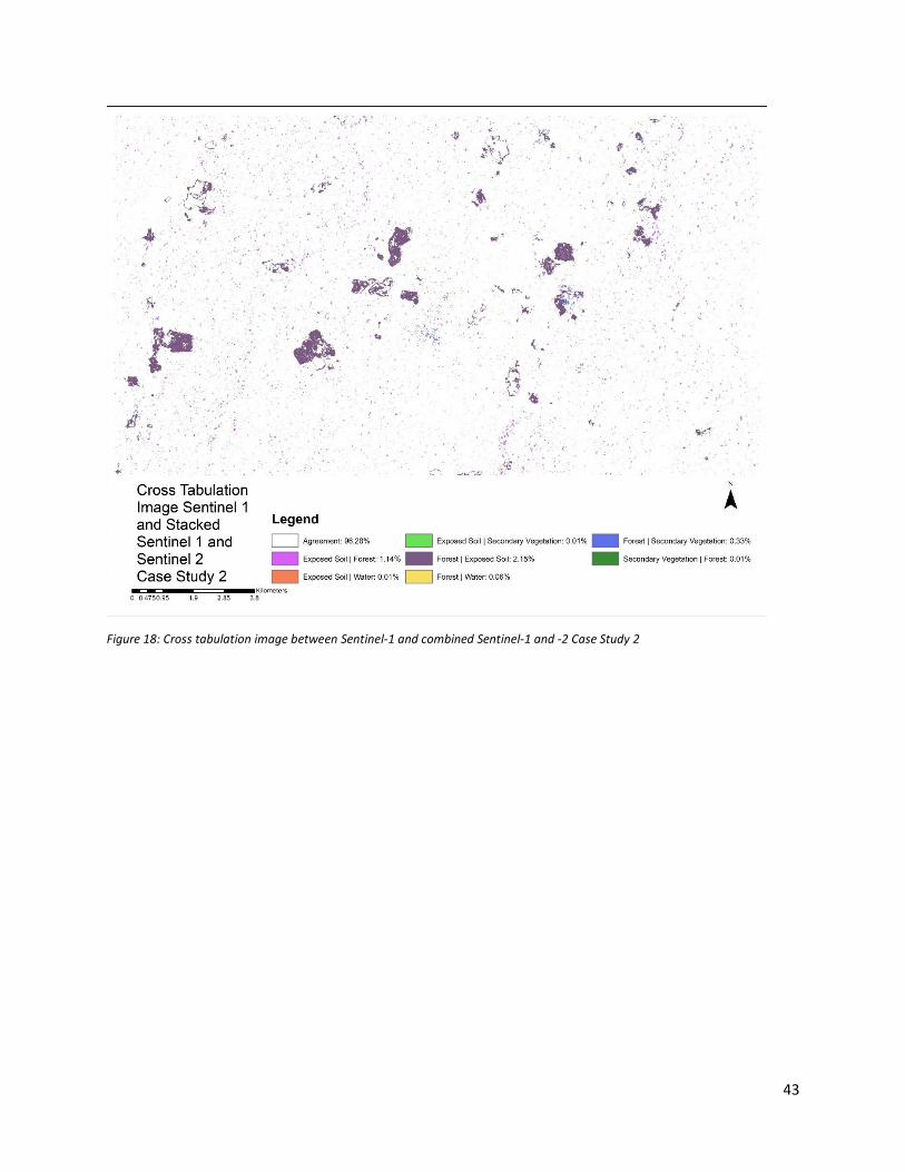
Overall, the disagreement between Sentinel-2 and the combined Sentinel-1 and -2 was low,

ranging from 1-4%. The low disagreement between these classifications, included the Sentinel-2 class of

forest being disaggregated into the classes of exposed soil, secondary vegetation, and water in the

Sentinel-1 and -2 classification images. The combined Sentinel-1 and -2 class of exposed soil was also

extracted from the Sentinel-2 class of secondary vegetation.

5.1 Discussion:

Overall, the mapping efficacy, as characterized by map and class accuracies, of Sentinel-1,

Sentinel-2, and Sentinel-1 and -2 varied across case studies but demonstrated the potential for Sentinel-

1 to delineate rough and smooth classes, Sentinel-2 to capture spectrally dissimilar classes, and for the

combination of Sentinel-1 and -2 to draw from both class roughness and multispectral qualities for

image classification.

The poor Sentinel-1 backscatter signature separability of classes with similar surficial roughness

resulted in high commission in the residential, secondary vegetation, and water classes, and high

omission in the forest and exposed soil classes. These high commission and omission errors were not as

prevalent in Sentinel-2. Sentinel-2 showed high map accuracy across all classes, but showed errors of

commission in the secondary vegetation class relating to omission in the class of exposed soil.

Combining Sentinel-1 and -2 created a classification image that benefited from the high multispectral

signature separability of the classes of residential and water and from the high backscatter signature

separability between the classes of secondary vegetation and exposed soil. Thus, the overall and class

accuracies were highest in the combined classification map that utilized both Sentinel-1 and -2.

23

Across images, there was nearly 85 – 95% similarity between the Sentinel-1 images and the

Sentinel-2 and combined Sentinel-1 and -2 images. The similarity between the Sentinel-2 images and the

combined Sentinel-1 and -2 images ranged from 95 – 99%. In case study 1, the majority of image

disagreement is in the disaggregation of the Sentinel-1 forest class into the Sentinel-2 classes of

residential, secondary vegetation, and exposed soil. The majority of disagreements between the

Sentinel-2 images and the combined Sentinel-1 and -2 images is seen in the class of secondary

vegetation, were the Sentinel-2 class of secondary vegetation is separated into the Sentinel-1 and -2

class of exposed soil. This disagreement between Sentinel-2 and the combined Sentinel-1 and -2

suggests that, given the increase in class accuracy from the Sentinel-2 secondary vegetation class to the

Sentinel-1 and -2 secondary vegetation class, integrating backscatter and multispectral signatures aids in

the delineation of secondary vegetation from exposed soil.

The speckled distribution of the Sentinel-1 exposed soil class in the Sentinel-2 class of forest, as

well as the disagreement between the Sentinel-2 class of exposed soil and Sentinel-1 class of forest,

describes classification disagreement likely due to SAR speckling artifacts. The apparent

mischaracterization of the Sentinel-1 class of exposed soil (and forest) is likely an artifact of the

constructive and destructive interference that defines homogenous land covers in SAR imagery (Smith,

2012). In this case, the scattering prevalent in homogenous areas results in highly heterogeneous

backscatter values, ranging from high intensity to low intensity (figure 1). While speckle filtering

mitigates this property of SAR images, the effect is not eliminated altogether, and thus, in study

confusion was introduced between classes that are separated based upon high and low backscatter

values (Smith, 2012).

This study adds to the body of work evaluating Sentinel-1 and Sentinel-2. Clerici et al. (2017)

observed, in a Colombian case study, map accuracies of random forest classifications for Sentinel-1

texture bands, Sentinel-2, and combined Sentinel-1 and-2 as 20.12%, 48.1%, and 55.5% respectively.

24

While from a differing region and using an alternate classification procedure (which had incorporated

texture bands of VV and VH as well as segmented training sites through eCognition), the classification

capabilities of Sentinel-1 and Sentinel-2 followed the same hierarchy as observed in this study, with the

integration of Sentinel-1 and -2 showing the highest overall accuracy followed by Sentinel-2 and then

Sentinel-1. In their work, the investigators were separating the classes of forests, secondary

vegetation/shrubs, cropland, water, pastureland, and built areas. The much lower classification

accuracies could be a result of the different classes evaluated, differences in the classification

procedures, or in non-stationarity across regions. It is likely that More case studies should be performed

to further characterize the performance of both Sentinel-1 and Sentinel-2 for land cover classification.

In this work, the Sentinel-1 classification accuracies across both case studies were lower than

the reported Sentinel-1 classification accuracies by Abdikan et al. (2017). Abdikan et al. (2017) evaluated

the classification potential of Sentinel-1 VV and VH polarization backscatter bands in Turkey. Abdikan et

al. (2017) showed overall map accuracies near 90% using a support vector machine classification of the

classes urban, water, forest, bare land, and agriculture. The large difference between the observed

Sentinel-1 classification accuracy in this study compared to the study conducted by Abdikan et al. (2017)

could be due to differences in scale, class sampling procedure, classification method, and or non-

stationarity of sensor performance.

This study argues, that Sentinel-1 could be useful for land cover mapping where weather

conditions prevent routine image acquisition and where class multispectral separability requires

additional information for delineating classes through scattering qualities, such as separating secondary

vegetation from bare ground. These benefits are contrasted against the extensive data preprocessing

requirements, the large data storage requirements, and processing time of SAR data. Compared to the

preprocessing requirements of optical imagery, preprocessing SAR is time consuming and

computationally expensive. Given these requirements for conducting SAR analysis, further work should

25

evaluate the effect of combining temporally neighboring Sentinel-1 images to determine how map

accuracies, specifically error due to the random speckle in homogenous land cover types, fluctuate with

the addition of backscatter information. Through characterizing how land cover classification accuracies

increase with increasing SAR images, an optimal number of images can be identified to maximize

accuracy while mitigating processing requirements.

Sentinel-2 demonstrated high accuracies for capturing high resolution land cover. Even with a

subset of the bands equipped on the MSI sensor, high map accuracies were achieved for fundamental

land cover classes of forest, exposed soil, water, residential, and secondary vegetation. Combined with

the relative ease of acquiring and preprocessing Sentinel-2 imagery through the SNAP software,

highlights the operational potential of the sensor for future land change monitoring projects, including

REDD+.

Together, Sentinel-1 and -2 are shown to benefit from their respective strengths, thereby

increasing overall map accuracy through class multispectral and backscatter characterization. The most

pronounced effect of combining the two sensors was the separation of the Sentinel-2 secondary

vegetation class into the combined Sentinel-1 and -2 exposed soil class. This highlights potential for

extraction of sparsely vegetated land cover from bare ground. Further work should explore the limits to

which the combination of Sentinl-1 and -2 benefits classifying a wider range of land cover types.

6. 1 Conclusion:

This study used Sentinel-1 and Sentinel-2 both individually and in tandem to create six land

cover classification maps along the border of the Pando department of Bolivia to evaluate their

respective classification capabilities. Using a random forest classifier to produce these images and

evaluating the end products through both general confusion matrices, Sentinel-1 proved useful to

generate simple land cover classifications based on landscape surficial roughness. The integration of

26

Sentinel-1 with Sentinel-2, increased map accuracy through characterizing classes through multispectral

and backscatter signatures. The most appropriate use of a single date non-textural classification of

Sentinel-1 backscatter values is over a landscape which has classes that are distinct in surficial

roughness, as it was predominantly between similarly textured classes that Sentinel-1 demonstrated the

greatest confusion. For a project with the goal of delineating forested areas from non-forested areas,

Sentinel-1 may be of significant use to classify landscapes often obscured by cloud cover and to act as

additional ancillary information to decrease overall map error.

Figures:

Table 1 Sensor Specifications for Sentinel-1 and Sentinel-2, the sensors evaluated and used in this study.

Sensor Spectral Resolution (bands) Temporal Resolution (days) Spatial Resolution (m)

Sentinel-1 C-Band 12 5 by 20 Sentinel-2 13 bands from VNIR to SWIR 5 10, 20, and 60

Table 2: Data Products and Parameters for the products used in this study.

Sensor Sentinel-2A Sentinel-1A

Name S2A_MSIL1C_20180904T144731_N0206_ R139_T19LFJ_20180904T182517

S1A_IW_GRDH_1SDV_20180906T10060 3_2018_0906T100630_023576_0291 75_6F5C

Acquisition Date September 4, 2018 September 6, 2018

Product Type S2 MSI Level-1C GRD

Bands 490 nm, 560 nm, 665 nm, 842 nm VV and VH

Mode IW

Pass Descending

Orbit 23576

Track 54

27

Figure 1: Study area map depicting the two case study locations, through Sentinel-1 VV, VH, and VV/VH RGB false color composites, in the Pando Department of Bolivia in the Northern region of the country sharing a border with Brazil. Forest is captured through the primary speckling depicted throughout the both images. Exposed soil and bare ground are captured in dark blue patches throughout the scene. Secondary vegetation is intermixed with subdued red and blue colorations. Water appears dark blue while some of the brightest pixels capture Residential areas as seen in Case Study 1 where there is a cluster of bright white pixels in the North central area of the scene.

28

Figure 2: Depicted above are the case study locations visualized through the conventional RGB false color composite using the Sentinel-2 Red, Green, and Near infrared bands. The dense forested landscape is depicted through varying shades of red to maroon. Secondary vegetation, which is a transitional class between low lying shrubbery and overgrown grasslands appears pink to light red in coloration for both images. The residential area in the municipality captured in the north central region of case study 1 is depicted as cyan to bright white. Exposed soil varies in coloration from highly reflective bright white and blue to a deeper green and gray color. The rivers, vary in coloration from each case study. In case study 1 there is a light blue color to the river with dark gray to black stagnant water sources nearby. In Case study 2, the river is much smaller and obscured by trees but stretches from the South central region of the study are across to the Northeast section of the study area and is seen through its dark grey coloration.

29

Figure 3: False Color Composites from Seninel-2 for case study 1 and case study 2, depicting final training sites.

30

Figure 4:Sentinel-1 SAR Backscatter Values for extracted by training sites for Case Study 1. The VH, VV, and difference backscatter images visualized across the from the respective boxplots highlight the large overlap in backscatter intensity between classes of similar textures. VH backscatter values typically are seen to be lower than the VV backscatter values across all classes, but demonstrate a similar pattern of class backscatter response where Forest, Vegetation (discussed in the paper using the term ‘Secondary Vegetation’), and Residential exhibit higher backscatter values on average than the bare ground and water classes.

31

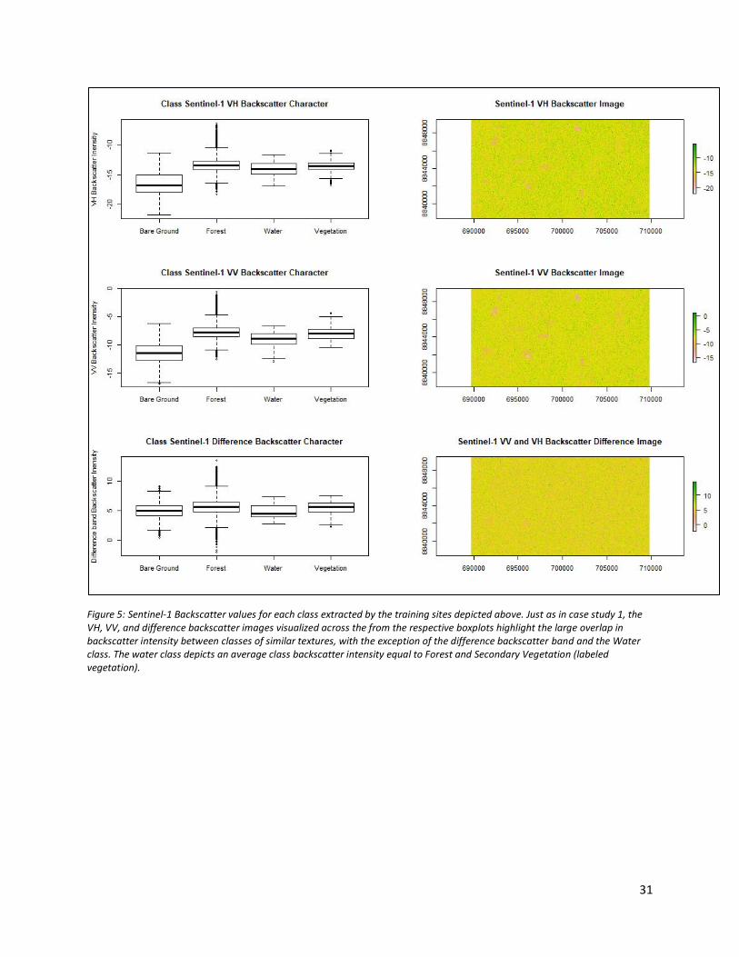
Figure 5: Sentinel-1 Backscatter values for each class extracted by the training sites depicted above. Just as in case study 1, the VH, VV, and difference backscatter images visualized across the from the respective boxplots highlight the large overlap in backscatter intensity between classes of similar textures, with the exception of the difference backscatter band and the Water class. The water class depicts an average class backscatter intensity equal to Forest and Secondary Vegetation (labeled vegetation).

32

Figure 6: Sentinel-2 mean reflectance values across the blue (492.4 nm), green (559.8 nm), red (664.6 nm), and near infrared (832.8 nm) bands for each class extracted by the training sites in case studies 1 and 2, shown in (A) and (B) respectively.

33

Figure 7: Random Forest Classification images for: (1) Sentinel-1 backscatter bands and backscatter difference band, (2) Sentinel-2 visible and near infrared optical bands, and (3) the combined Sentinel-1 backscatter and Sentinel-2 optical bands in Case Study 1. Individual random forest models were trained and used to predict land cover for each classification separately. The training incorporated every pixel provided through the training data and used 1000 decision trees.

34

Figure 8: Random Forest Classification images for: (1) Sentinel-1 backscatter bands and backscatter difference band, (2) Sentinel-2 visible and near infrared optical bands, and (3) the combined Sentinel-1 backscatter and Sentinel-2 optical bands in Case Study 2. Identical to case study 1, Individual random forest models were trained and used to predict land cover for each classification separately using 1000 decision trees.

35

Figure 9: Case 1 Accuracy Assessment points for each classification image. Due to spatial differences between the classes captured in the Sentinel-1 image vs the Sentinel-2 and combined Sentinel product, each accuracy assessment was independently created and evaluated.

36

Figure 10: Case study 2 accuracy assessment points for each classification image. While the spatial allocation of classes remained largely different between the Sentinel-1 classification image and the other two classifications, the Sentinel-2 and combined Sentinel image were coincident enough in class allocation to use the same stratified sample points for each image while preserving the equal class sampling.

37

Figure 11: Case 1 and 2 overall accuracies calculated through a confusion matrix of the stratified randomly sampled points possessing ground truth class information and classification image designations. The percent overall accuracy is a calculation of the number of points that observed the same image class and ground truth class designations divided by the total number of samples points. In both case studies, the Sentinel-1 images showed lower overall percent correct than the Sentinel-2 and combined Sentinel-1 and Sentinel-2 images.

38

Figure 12: Case 1 class accuracies calculated through a confusion matrix of the sampled points possessing ground truth class information and classification image designations. The class accuracy is a calculation of the number of points that observed the same image class and ground truth class designations divided by the total number of samples in that class.

Figure 13: Case 1 class accuracies calculated through a confusion matrix of the sampled points possessing ground truth class information and classification image designations. The class accuracy is a calculation of the number of points that observed the same image class and ground truth class designations divided by the total number of samples in that class.

39

Figure 14: Cross tabulation of Sentinel-1 and Sentinel-2 Images Case 1 depicting areas of disagreement by proportion of entire image.

40

Figure 15: Cross tabulation of Sentinel-1 and combined Sentinel-1 and -2, showing areas of disagreement by proportion of Image.

41

Figure 16: Cross tabulation of Sentinel-2 and combined Sentinel-1 and Sentinel-2, showing areas of disagreement by proportion of Image.

42

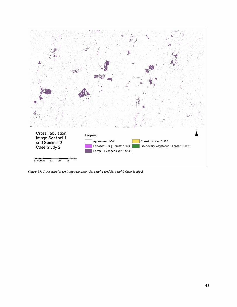
Figure 17: Cross tabulation image between Sentinel-1 and Sentinel-2 Case Study 2

43

Figure 18: Cross tabulation image between Sentinel-1 and combined Sentinel-1 and -2 Case Study 2

44

Figure 19: Cross tabulation image between Sentinel-2 and combined Sentinel-1 and -2 Case Study 2

7.1 Appendix:

Table 3: Case 1 Summary Table of Accuracy Assessment Results from 250 points. Errors of Omission and Commission are reported as well as image overall accuracy.

Sentinel-1 Sentinel-2 Sentinel-1 and-2

Class Commission

Error Omission

Error Commission

Error Omission

Error Commission

Error Omission

Error

Forest 10% 52% 8% 15% 11% 11%

Secondary Vegetation 60% 29% 58% 40% 46% 43%

Residential 70% 25% 26% 7% 23% 7%

Water 48% 16% 4% 14% 0% 18%

Exposed Soil 32% 29% 32% 48% 31% 31%

Overall Accuracy: 56% 74% 78%

45

Table 4: Case 2 Summary Table of Accuracy Assessment Results from 200 Points. Errors of Omission and Commission are reported as well as image overall accuracy.

Sentinel-1 Sentinel-2 Sentinel-1 and 2

Class Commission

Error Omission

Error Commission

Error Omission

Error Commission

Error Omission

Error

Forest 6% 70% 34% 51% 24% 44%

Secondary Vegetation

98% 83% 56% 29% 46% 31%

Water 94% 0% 28% 28% 24% 14%

Exposed Soil 50% 26% 10% 12% 14% 14%

Overall Accuracy: 38% 68% 73%

Table 5: Confusion Matrix for Case Study 1

Sentinel-1 Forest Soil Residential Water Secondary Vegetation Total

User Accuracy

Forest 45 1 1 0 3 50 0.90 Soil 6 34 4 4 2 50 0.68 Residential 21 10 15 1 3 50 0.30 Water 0 24 0 26 0 50 0.52 Secondary Vegetation 22 8 0 0 20 50 0.40 Total 94 77 20 31 28 250 0 Producer Accuracy 0.48 0.44 0.75 0.84 0.71 0 0.56

Sentinel-2 Forest Soil Residential Water Secondary Vegetation Total

User Accuracy

Forest 46 0 0 1 3 50 0.92

Soil 1 34 3 3 9 50 0.68

Residential 0 9 37 2 2 50 0.74 Water 2 0 0 48 0 50 0.96 Secondary Vegetation 5 22 0 2 21 50 0.42 Total 54 65 40 56 35 250 0 Producer Accuracy 0.85 0.52 0.93 0.86 0.60 0 0.74

Combined Sentinel-1 and -2 Forest Soil Residential Water

Secondary Vegetation Total

User Accuracy

Forest 48 0 0 3 3 54 0.89 Soil 1 45 3 6 10 65 0.69 Residential 0 9 37 0 2 48 0.77 Water 0 0 0 46 0 46 1

Secondary Vegetation 5 11 0 1 20 37 0.54

Total 54 65 40 56 35 250 0 Producer Accuracy 0.89 0.69 0.93 0.82 0.57 0 0.78

Table 6: Confusion Matrix Case Study 2

46

Sentinel-1 Exposed Soil Forest Water Secondary Vegetation Total

User Accuracy

Exposed Soil 25 24 0 1 50 0.50

Forest 0 47 0 3 50 0.94

Water 5 41 3 1 50 0.06

Secondary Vegetation 4 45 0 1 50 0.02

Total 34 157 3 6 200 0

Producer Accuracy 0.74 0.30 1 0.17 0 0.38

Sentinel-2 Exposed Soil Forest Water Secondary Vegetation Total

User Accuracy

Exposed Soil 45 3 0 2 50 0.90

Forest 0 33 14 3 50 0.66

Water 6 4 36 4 50 0.72

Secondary Vegetation 0 28 0 22 50 0.44

Total 51 68 50 31 200 0

Producer Accuracy 0.88 0.49 0.72 0.71 0 0.68

Combined Sentinel-1 and -2 Exposed Soil Forest Water

Secondary Vegetation Total

User Accuracy

Exposed Soil 43 5 1 1 50 0.86

Forest 0 38 5 7 50 0.76

Water 7 2 37 4 50 0.74

Secondary Vegetation 0 23 0 27 50 0.54

Total 50 68 43 39 200 0

Producer Accuracy 0.86 0.56 0.86 0.69 0 0.73

Table 7: Cross Tabulation of Images, Case Study 1

Cross Tabulation of Sentinel-1 (Columns) and Sentinel-2 (Rows)

Category Forest Exposed Soil Residential Water Secondary Vegetation Total

Forest 264995 5773 1572 71 1804 274215

Soil 17949 19524 970 435 796 39674

Residential 5105 2718 743 70 165 8801

Water 254 1637 17 376 25 2309

Secondary Vegetation 15144 3488 296 43 550 19521

Total 303447 33140 3598 995 3340 344520

Cross Tabulation of Sentinel-1 (Columns) and Combined Sentinel-1 and-2 (Rows)

Category Forest Exposed Soil Residential Water Secondary Vegetation Total

Forest 264130 5392 1548 59 1778 272907

Exposed Soil 13316 22840 919 483 791 38349

Residential 5771 2131 851 30 153 8936

Water 80 1627 9 415 22 2153

Secondary Vegetation 20150 1150 271 8 596 22175

Total 303447 33140 3598 995 3340 344520

47

Cross Tabulation of Sentinel-2 (Columns) and Combined Sentinel-1 and -2 (Rows)

Category Forest Exposed Soil Residential Water Secondary Vegetation Total

Forest 271592 392 0 118 805 272907

Exposed Soil 268 32460 906 129 4586 38349

Residential 0 1031 7857 48 0 8936

Water 19 94 37 2000 3 2153

Secondary Vegetation 2336 5697 1 14 14127 22175

Total 274215 39674 8801 2309 19521 344520

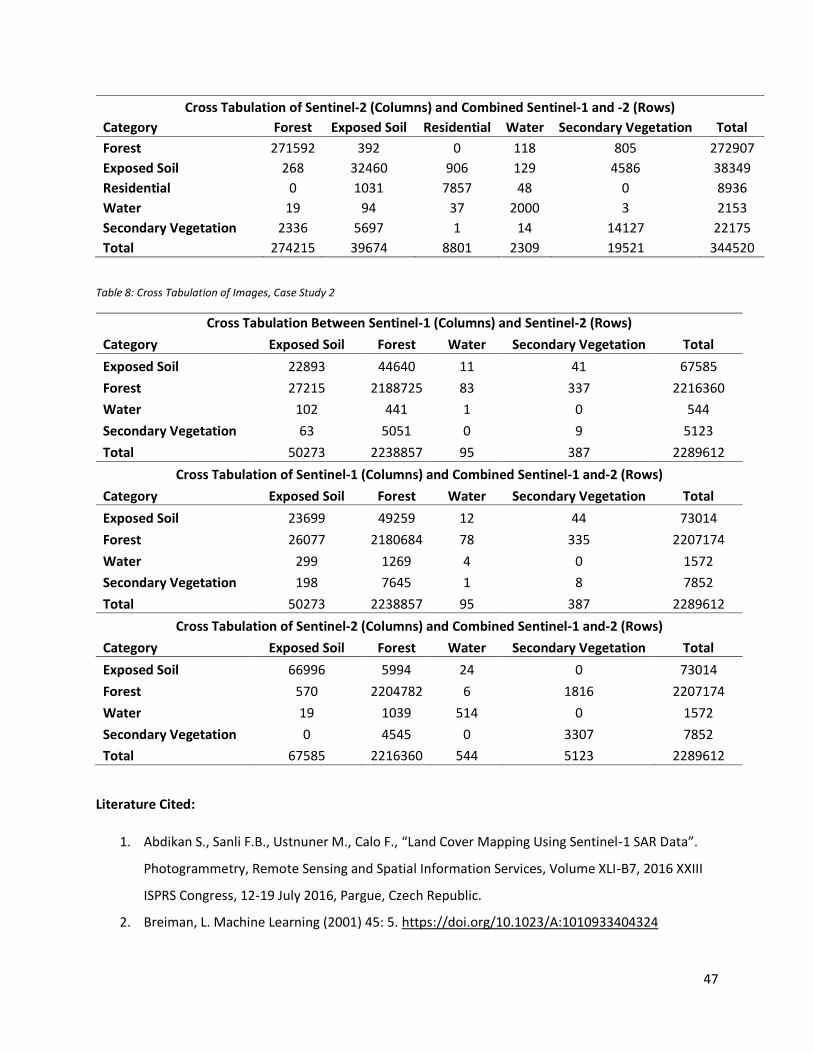
Table 8: Cross Tabulation of Images, Case Study 2

Cross Tabulation Between Sentinel-1 (Columns) and Sentinel-2 (Rows)

Category Exposed Soil Forest Water Secondary Vegetation Total

Exposed Soil 22893 44640 11 41 67585

Forest 27215 2188725 83 337 2216360

Water 102 441 1 0 544

Secondary Vegetation 63 5051 0 9 5123

Total 50273 2238857 95 387 2289612

Cross Tabulation of Sentinel-1 (Columns) and Combined Sentinel-1 and-2 (Rows)

Category Exposed Soil Forest Water Secondary Vegetation Total

Exposed Soil 23699 49259 12 44 73014

Forest 26077 2180684 78 335 2207174

Water 299 1269 4 0 1572

Secondary Vegetation 198 7645 1 8 7852

Total 50273 2238857 95 387 2289612

Cross Tabulation of Sentinel-2 (Columns) and Combined Sentinel-1 and-2 (Rows)

Category Exposed Soil Forest Water Secondary Vegetation Total

Exposed Soil 66996 5994 24 0 73014

Forest 570 2204782 6 1816 2207174

Water 19 1039 514 0 1572

Secondary Vegetation 0 4545 0 3307 7852

Total 67585 2216360 544 5123 2289612

Literature Cited:

1. Abdikan S., Sanli F.B., Ustnuner M., Calo F., “Land Cover Mapping Using Sentinel-1 SAR Data”.

Photogrammetry, Remote Sensing and Spatial Information Services, Volume XLI-B7, 2016 XXIII

ISPRS Congress, 12-19 July 2016, Pargue, Czech Republic.

2. Breiman, L. Machine Learning (2001) 45: 5. https://doi.org/10.1023/A:1010933404324

48

3. UNFCCC. 2014. Key decisions relevant for reducing emissions from Deforestation and forest

degradation in developing countries (REDD+). Decision Booklet REDD+. UNFCCC Publication:

Bonn, Germany.

4. Bourg, L. (2009): MERIS Level 2 Detailed Processing Model. ACRI-ST, Document No. PO-TN-MEL-

GS-0006, 15 July 2009.

5. Nicola Clerici, Cesar Augusto Valbuena Calderón & Juan ManuelPosada (2017) Fusion of

Sentinel-1A and Sentinel-2A data for land cover mapping: a casestudy in the lower Magdalena

region, Colombia, Journal of Maps, 13:2, 718-726, DOI:10.1080/17445647.2017.137231

6. Chuvieco Emilio. 2016. Fundamentals of Satellite Remote Sensing: An Environmental Approach.

Second Edition. Taylor & Francis Group. Boca Raton, Florida. 2016.

7. Dostálová Alena, Hollaus Markus, Milenković Milutin, and Wagner Wolfgang (2016). Forest area

derivation from Sentinel-1 data. Remote Sensing and Spatial Information Sciences, 3:7, 12-19,

DOI: 10.5194/isprs-annals-III-7-227-2016

8. "ESA, Copernicus, Overview". ESA. 28 October 2014. Retrieved 26 April 2016.

9. Yolanda Fernandez-Ordonez, Jesus Soria-Ruiz and Brigitte Leblon (2009). Forest Inventory using

Optical and Radar Remote Sensing, Advances in Geoscience and Gemote Sensing, Gary Jedlovec

(Ed.), ISBN: 978-953-307-005-6, InTech, Available from:

http://www.intechopen.com/books/advances-in-geoscience-and-remote-

sensing/forestinventory-using-optical-and-radar-remote-sensing

10. Gerald Forkuor, Kangbeni Dimobe, Idriss Serme & Jerome Ebagnerin Tondoh (2018) Landsat-8

vs. Sentinel-2: examining the added value of sentinel-2’s red-edge bands to land-use and land-

cover mapping in Burkina Faso, GIScience & Remote Sensing, 55:3, 331-354, DOI:

10.1080/15481603.2017.1370169

11. Funning, G. (2018). Insar Theory and Processing [Powerpoint slides]. Retrieved from:

https://www.unavco.org/education/professional-development/short-courses/2018/insar-

training-gsa/insar-training-gsa.html

12. Google earth V 6.2.2.6613. (July , 2018). Pando Department, Bolivia. 10° 25’ 35.27”S,

67° 27’ 51”W, Eye alt 29 mi. DigitalGlobe 2018. http://www.earth.google.com

[September, 2018].

13. Global forest resources assessment 2015: Desk reference. FAO. Book. URI:

http://www.fao.org/3/a-i4808e.pdf · http://hdl.handle.net/20.500.11822/19698.

49

14. M. Hansen, R. Dubaya & R. Defries (1996) Classification trees: an alternative to traditional land

cover classifiers, International Journal of Remote Sensing, 17:5, 1075-1081, DOI:

10.1080/01431169608949069

15. Barry Haack and Ron Mahabir (2018) Relative value of radar and optical data for land cover/use

mapping: Peru example, International Journal of Image and Data Fusion, 9:1, 1-20, DOI:

10.1080/19479832.2017.1398188

16. Terry Idol, Barry Haack, and Ron Mahabir (2015) Comparison and integration of spaceborne

optical and radar data for mapping in Sudan, International Journal of Remote Sensing, 36:6,

1551-1569, DOI: 10.1080/014131161.2015.1015659

17. Kasischke, E. S., Melack, J. M., & Dobson, M. C. (1997). The use of imaging radars for ecological

applications—A review. Remote Sensing of Environment,59,141−156.

18. Laur H., Bally P., Meadows P., Sïnchez J., Schïttler B., Lopinto E. & Esteban D., ERS SAR

Calibration: Derivation of σ0 in ESA ERS SAR PRI Products, ESA/ESRIN, ES-TN-RS-PM-HL09, Issue

2, Rev. 5f, November 2004

19. Lee, J.-S., Jurkevich, I., Dewaele, P., Wambacq, P., and A. Oosterlinck, 1994, “Speckle Filtering of

Synthetic Aperture Radar Images: A Review,” Remote Sensing Review, 8:313-340.

20. Lee, J.S., 1981. Speckle Analysis and Smoothing of Synthetic Aperture Radar Images. Computer

Graphics and Image Processing, Vol. 17:24-32.

21. Li L., Roy D., (2017). A Global Analysis of Sentinel-2A, Sentinel-2B, and Landsat-8 Data Revisit

Intervals and Implications for Terrestrial Monitoring. Remote Sensing.9, 902; doi:

10.3390/rs9090902. www.mdpi.com/journal/remotesensning.

22. Mansourpour M., Rajabi M.A., Blais J.A.R., 2006, “Effects and Performance of Speckle Noise

Reduction Filters on Active Radar and SAR Images”,

http://people.ucalgary.ca/~blais/Mansourpour2006.pdf

23. Morley, R. J. 2000. Origin and Evolution of Tropical Rain Forests, Chichester: John Wiley and

Sons. p. 362, 378.

24. Müller R, Pacheco P and Montero JC. 2014. The context of deforestation and forest degradation

in Bolivia: Drivers, agents and institutions. Occasional Paper 108. Bogor, Indonesia: CIFOR.

25. Mitchell A, Rosenqvist A, Mora B. 2017. Current remote sensing approaches to monitoring

forest degradation in support of countries measurement, reporting and verification (MRV)

systems for REDD+. Carbon Balance and Management. Published Online. 17 April 2017.

50

26. Magangoz A., Sekertekin A., Akcin H. “Analysis of Land Use Land Cover Classification Results

Derived From Sentinel-2 Image”. Photogrammetry and Remote Sensing. 2017.

27. M. Mahmudur Rahmanm, Tetuko Sri Sumantyo J., “Mapping Tropical Forest Cover and

Deforestation Using Synthetic Aperature Radar (SAR) Images”. Appl Geomat (2010) 2:113-121.

DOI: 10.1007/s12518-010-0026-9.

28. E. Mandanici and G. Bitelli., (2016) “Preliminary Comparison of Sentinel-2 and Landsat 8 Imagery

for a Combined Use”. Remote Sensing, 8, 1014. Doi:10.3390/rs8121014.

29. Kuhn, M. (2008). Building Predictive Models in R Using the caret Package. Journal of Statistical

Software, 28(5), 1 - 26. doi:http://dx.doi.org/10.18637/jss.v028.i05

30. Pistorius T. From RED to REDD+: the evolution of a forest-based mitigation approach for

developing countries. Curr Opin Environ Sustain. 2012;4(6):638-45.

31. Qiu F., Berglund J., Jensen J., Thakkar P., and Ren D., 2004, “Speckle Noise Reduction in SAR

Imagery Using a Local Adaptive Median Filter”. GIScience and Remote Sensing, Vol. 41:244-266.

32. Johannes Reiche, Eliakim Hamunyela, Jan Verbesselt, Dirk Hoekman, Martin Herold (2018)

Improving near-real time deforestation monitoring in tropical dry forests by combining dense

Sentinel-1 time series with Landsat and ALOS-2 PALSAR-2. Remote Sensing of Environment, 204:

147-161.

33. SNAP - ESA Sentinel Application Platform v6.0.5, http://step.esa.int

34. Sawaya, S., B. Haack, T. Idol, and A. Sheoron. 2010. “Land Use/Cover Mapping with Quad-

Polarization RADAR and Derived Texture Measures Near Wad Madani, Sudan.” GIScience &

Remote Sensing 47 (3): 398-411. Doi: 10.2747/1548-1603.47.3.398

35. Shearon, A., and B. Haack. 2013. “Classification of California Agriculture using Quad Polarization

Radar Data and Landsat Thematic Mapper Data.” GIScience and Remote Sensing 50 (1): 50-63.

Doi: 10.1080/15481603.2013.778555.

36. Smith, R. B. 2012. Interpreting Digital Radar Images with Tntmips, 20. Lincoln, NE: MicroImages.

37. Sentinel-1 Observation Scenario. Web Access 4/12/2018. url:

https://sentinel.esa.int/web/sentinel/missions/sentinel-1/observation-scenario

38. Sentinel-2 Revisit and Coverage. Web Access 4/12/2018. url:

https://earth.esa.int/web/sentinel/user-guides/sentinel-2-msi/revisit-coverage

39. Skinner B. and Murck B. (2011). “The Blue Planet: an introduction to earth system science”. John

Wiley & Sons, Inc.

40. Small D., Schubert A., Guide to ASAR Geocoding, RSL-ASAR-GC-AD, Issue 1.0, March 2008

51

41. Suhet, B. Hoersch, “Sentinel-2 User Handbook” (2015). European Space Agency (ESA).

https://sentinel.esa.int/documents/247904/685211/Sentinel-2_User_Handbook

42. Schmullius, C.; Thiel, C.; Pathe, C.; Santoro, M. Radar time series for land cover and forest

mapping. In Remote Sensing Time Series; Kuenzer, C., Dech, S., Wagner, W., Eds.; Remote

Sensing and Digital Image Processing; Springer International Publishing: Basel, Switzerland,

2015; pp. 323–356

43. Violini Soraya., (2013). Deforestation: Change Detection in Forest Cover Using Remote Sensing.

Maio-Gulich Insitute, CONAE. Argentina.

44. Thanh Noi, P.; Kappas, M. Comparison of Random Forest, k-Nearest Neighbor, and Support

Vector Machine Classifiers for Land Cover Classification Using Sentinel-2 Imagery. Sensors 2018,

18, 18.

45. Thiel, C.; Cartus, O.; Eckardt, R.; Richter, N.; Thiel, C.; Schmullius, C. Analysis of multi-temporal

land observation at C-band. In Proceedings of the 2009 IEEE International Geoscience and

Remote Sensing Symposium (IGARSS), Cape Town, South Africa, 12–17 July 2009;

doi:10.1109/IGARSS.2009.5417764.

46. Waske B., Braun M., Classifier ensembles for land cover mapping using multitemporal SAR

imagery (2009), Journal of Photogrammetry and Remote Sensing, 64:5, 450-457,

https://doi.org/10.1016/j.isprsjprs.2009.01.003

47. T. Warner, M. Nellis, G. Foody, (2009) “The SAGE Handbook of Remote Sensing”. SAGE

Publications Ltd.

48. Wang, B.; Jia, K.; Liang, S.; Xie, X.; Wei, X.; Zhao, X.; Yao, Y.; Zhang, X. Assessment of Sentinel-2

MSI Spectral Band Reflectances for Estimating Fractional Vegetation Cover. Remote Sens. 2018,

10, 1927.