1

An Evaluation of Financial Institutions: Impact on

Consumption and Investment Using Panel Data and the

Theory of Risk-Bearing*

Mauro Alem, Banco de Inversiones y Comercio Exterior (BICE)

Robert M. Townsend, Dept. of Economics, MIT†

Revised April 26, 2012

Abstract

The theory of the optimal allocation of risk and the Townsend Thai panel data on

financial transactions are used to assess the impact of the major formal and informal

financial institutions of an emerging market economy. We link financial institution

assessment to the actual impact on clients, rather than ratios and non-performing loans.

We derive both consumption and investment equations from a common core theory with

both risk and productive activities. The empirical specification follows closely from this

theory and allows both OLS and IV estimation. We thus quantify the consumption and

investment smoothing impact of financial institutions on households including those

* Research support from the National Institutes of Health, the National Science Foundation, the John Templeton Foundation, the Consortium on Financial Systems and Poverty at the University of Chicago, and the Ford Foundation are gratefully acknowledged. We thank the National Statistic Office of Thailand for permission to use their data. We gratefully acknowledge Hoai-Luu Quang Nguyen, Ananth Ramanarayanan, Carlos Perez-Verdia, Kaveh Hemmat and John Felkner for able research assistance. Helpful comments from participants of the MIT development lunch group, the Chicago econometrics workshop, and the IMF conference on structural reforms and poverty, and especially from Joshua Angrist, Abhijit Banerjee, Esther Duflo, Michael Greenstone, and Joseph Kaboski are all greatly acknowledged. In addition, we thank the editor and referees who helped to make substantial improvements. † Corresponding Author: Department of Economics, MIT, 77 Mass. Ave, E52-252c, Cambridge, MA 02139, USA, Tel: +1-617-452-3722, email: rtownsen@mit.edu.

2

running farms and small businesses. A government development bank (BAAC) is shown

to be particularly helpful in smoothing consumption and investment, in no small part

through credit, consistent with its own operating system, which embeds an implicit

insurance operation. Commercial banks are smoothing investment, largely through

formal savings accounts. Other institutions seem ineffective by these metrics.

JEL Codes: G2, O16, R1

Keywords: Financial Institutions; Risk Sharing; Evaluation; Economic Welfare

3

1. Introduction

There has been little theory-based assessment of formal and informal financial

institutions which uses not only financial statements and institutional detail but also

household panel data on actual customers. Here we explicitly incorporate the diversity of

shocks across households in an environment with productive opportunities in a choice

model of financial participation. We use the theory of an optimal allocation of risk-

bearing to derive both consumption and investment equations for customers of financial

institutions. We also do the same for those in financial autarky. Finally, we make

participation endogenous and evaluate the formal and informal financial institutions that

offer savings, credit and insurance.

We make use of the Townsend Thai data, a panel of approximately 960

households, including about 200 running their own businesses. The data start in May

1997, just prior to the onset of the July 1997 financial crisis, and continue through 2001,

that is, through the recovery. Thus there is macro, aggregate risk.1 The data are gathered

from households and small businesses specialized in different mixes of occupations and

subject to different shocks. Thus, there is ample idiosyncratic risk.2 The data contain the

measurements of consumption, investment, and income necessary to carry out the 1 In the working paper version (Alem and Townsend, 2004), we show that consumption drops across both surveyed regions in the first three years. Surprisingly however, the few statistically significant common time effects in income over households explain little of the income variation. Droughts, floods and price changes are events that drive much income change according to the surveyed households, but these are not uniform within and across regions. 2 In the working paper version (Alem and Townsend, 2004), we show that wage earners and those in agriculture suffered lower declines in income than anticipated in the Thai government’s policy response, and business owners suffered large declines in income on average. Within each of the occupation groups there is enormous heterogeneity income change.

4

standard risk-bearing or equivalent-with-complete-market tests. Further, the data record

the actual use of formal and informal financial institutions and mechanisms by type of

financial product, both borrowing and saving. From this we can see which devices are

used and gauge the plausibility of econometric instruments for subsequent actual

participation. The instruments are derived from a baseline key informant interviews and

from a baseline 1996 village-level census from the Community Development Department

(CDD). One of the instruments makes use of a Geographic Information System (GIS).

The principal findings offer a score card or rating system for the major financial

institutions of the country. A government development bank (BAAC) is shown to be

particularly helpful in smoothing consumption and investment, in no small part through

credit, consistent with its own operating system, which embeds an implicit insurance

operation. Commercial banks are smoothing investment, largely through formal savings

accounts. Other institutions seem ineffective by these metrics

The paper is outlined as follows. Section 2 describes the data used in the analysis.

In Section 3, we present the basic choice model of financial regimes featuring the

assumed environment. In Section 4, we derive from the theory of optimal allocation of

risk the explicit consumption and investment equations used in the empirical work. In

Section 5, we do the same for those in financial autarky. In Section 6, we derive the

econometric specification, including how we use the data and our instruments. The

assessed impact of each major financial institution is summarized in Section 7. Section 8

provides additional results and interpretation. Section 9 concludes.

2. Data and Institutions

5

The panel data used in this paper come from a project funded by the National

Institutes of Health, the National Science Foundation, and the Ford Foundation (see

Townsend, 1997). An initial cross-sectional survey, with retrospective data, was fielded

in May, 1997, before the crisis that began with the devaluation of the Thai baht in July,

1997. Two regions were chosen deliberately: namely, the more developed Central region

and the relatively poor, semi-arid Northeast. Within each region two provinces were

chosen deliberately as each had at least one county (amphoe) that had been randomly

selected in all previous rounds of the larger Socio-Economic Survey (SES). In the Central

region the province of Chachoengsao is adjacent to Bangkok and contains an industrial

corridor that makes its way to the eastern seaboard. The province of Lopburi is in the

fertile central valley north of Bangkok. In the Northeast, the province of Sisaket is the

poorest in Thailand according to provincial product data, and Buriram, also in the

Northeast, represents a transition province as one moves west back toward Bangkok.

Within each province twelve tambons or sub-counties were chosen at random (see

Binford, Lee, and Townsend, 2004). Within each tambon, four villages were chosen at

random from an enumeration of villages available from the Community Development

Department (CDD), and within each village fifteen households were chosen at random

from a listing held by the headman.3 In addition to the household questionnaire, survey

instruments were designed for the headman of each village, soliciting in particular a

retrospective village history of the use of formal and quasi-formal financial institutions.

3 The mean and median numbers of villages in a tambon are 10.38 and 10.0 respectively. Thus, the fraction of villages chosen from the total is approximately 40%. The sampling rate for tambons in a province is 3% and the sampling rate for households in a village is 11%.

6

With the advent of the crisis, funding from the Ford Foundation allowed a

resurvey one year later (in May, 1998) of one-third of the original sample, and this was

continued with NICHD funding into subsequent years. The data used in this paper is

through 2001. For this Townsend Thai resurvey panel, four tambons were chosen at

random from the original twelve of each province.4 Otherwise, the same villages and the

same households were selected for re-interviews. The target number of households was

960, or 240 in each province. The actual response rate for this 1997-1998 pairing is

relatively high, for example, 98.2% of the target 1997 households respond again to the

resurvey. Likewise, there were successful re-interviews of 96.2%, 97.1% and 96.5% for

the other pairs of years. Tables A.1 and A.2 in the appendix contain a summary of key

variables used in the data analysis.

Measurement of income, consumption and investment. We note that income is

measured as the difference between gross income and gross expenses, solicited from the

household for each occupation category separately: business, agriculture, fish/shrimp,

farming and livestock. Labor income is gross revenue from wages. Likewise, all physical

assets held at each interview date are solicited along with purchase date and value at that

time. Discrepancies in ownership across interviews are checked and reconciled with the

households directly. Depreciation rates, e.g., 10%, can be applied to create retrospective

panel data on wealth. There are, in addition, direct questions on land sales and

acquisitions, the major asset in many cases (this is not depreciated). Consumption is

4 With the exception that one tambon was set aside for a separate intensive monthly survey.

7

measured by a solicitation of 13 items5 that best predict aggregated non-durable

consumption expenditure in the larger more comprehensive Socio-Economic Survey. In

practice, 50-80% of the variation can be explained by these 13 items. A price index at the

province level was obtained using average prices of purchases of consumption in order to

deflate and express income, consumption and investment in real terms.6 Specifically, the

Townsend Thai annual data records both the overall value and quantity of the first 9

consumption items purchased by each surveyed household. There is a considerable range

for these deduced prices for a given year and province, and so in order to reduce

measurement error and provide a reliable overall central tendency, the top and bottom

25% of the histogram for each item are removed, then a simple average is taken. The

overall price index is constructed by weighting each price item by its quantity in the base

year (Laspeyres).

Measurement of financial participation. Membership in or being a customer of

the various financial institutions was solicited in the 1997 interview, along with a

retrospective history. Hence, we know in principle if a household was using a

commercial bank in, for example, the 1996 baseline year, the year prior to the survey. We

also have measurements of all subsequent financial transactions (borrowing, lending,

saving) with the formal sector (type of institution, e.g., BAAC, village funds such as

Production Credit Groups [PCGs], commercial banks) and with the informal sector

5 Grain, milk and milk products, meat, alcohol consumed at home, alcohol consumed away, tobacco, gasoline, ceremonies, house repairs, vehicle repairs, educational expenses, clothing and meals away from home. 6 As a robustness check, a national deflator price index was obtained from the National Statistics Office and the results, though statistically weaker, did not vary in sign and order of magnitude.

8

(output purchaser, money lender, friends, relatives, store owners). There are also data on

remittances and the use of rice in storage.

Financial institutions overview. We emphasize here that we have the typical

array of financial institutions of emerging market economies: government banks, local

savings and loans, a private (but regulated) commercial banking sector and, again, a

substantial informal sector.

BAAC is the Thai government’s Bank for Agriculture and Agricultural

Cooperatives. It makes modestly sized loans, about half with joint liability and hence no

physical collateral. Its interest rate is slightly subsidized, and the BAAC could break even

by raising its on-lending rate only a modest amount (Yaron, 1994). The BAAC does

compete actively for savings deposits (as commercial banks are no longer required to

deposit funds). Though nominally lending to agriculture (fertilizer, seed), business

households in the Townsend Thai survey sometimes report that they get initial funding

from the BAAC. Most loans are short term, but long term investment is also possible.

The BAAC has focused on getting credit to a certain segment of farmers, and in the data

it appears they are more willing to lend off the main road, away from towns. The BAAC

had 34% of all loans outstanding in the larger 1997 baseline survey and focuses on the

middle wealth segment of the market in each village. Townsend and Yaron (2001) have

featured the “risk-contingency” nature of lending, in which delayed repayment and

possibly reduced interest and/or principal is part of the BAAC operating system. This

presumably is a mechanism which would allow mitigation of idiosyncratic shocks,

though that has not been tested previously.

9

Commercial banks make relatively few loans in the Townsend Thai peri-urban

data, 3% of all loans in the 1997 data, but loan size is relatively large, larger than all other

lenders. So, by value, commercial banks have 16% of all loans. Bank lending is clustered

in the sense that if a commercial bank is active in a village, it is likely to be active nearby,

and there remain plenty of gaps. Virtually all commercial bank loans require collateral.

On the other hand, commercial bank savings account for 56% of all savings, especially

for higher wealth households and those in more developed regions.

Agricultural Cooperatives are now part of the Bank for Agriculture and

Agricultural Cooperatives, but many retain their former quasi-independent status, run by

local boards and so on. The BAAC on-lends to Cooperatives and historically suffers a

lower repayment rate than with direct loans to customers.

Village level financial institutions appear frequently. One of the more common

types is a Production Credit Group, essentially a local savings and loan run by a village

committee. There are also women’s groups, rice banks, buffalo banks, poverty

eradication funds, and others, though sample size in the annual panel did not allow us to

do much with these.7 The well-known and larger One Million Baht Village Funds,

analyzed in Kaboski and Townsend (2011; 2012) were not introduced until 2002, and we

do not use that data here.

The informal sector comprises approximately half of all loans, not only from

money lenders but also from store keepers, traders, friends, relatives, and so on. There is

great variety in collateral, interest rates and repayment. We also think of rice storage as

7 See Kaboski and Townsend (2005) for a more detailed description and analysis using the 1997 data.

10

an activity of the informal sector, distinct from savings in commercial banks or the

BAAC. Rice accounts for 14% of all savings (excluding the value of cash, gold, and

jewelry which are not measured in the annual data).

Instruments for financial participation. We also employ the CDD data, a

comprehensive village-level census and the key informant questionnaire to obtain

instruments for membership of formal and informal institutions: (i) key informant

responses regarding the availability of productive credit in the village from various

specific financial institutions; (ii) travel times to district centers as measured in CDD

data; and (iii) GIS-calculated probabilities based on CDD neighborhood averages that a

village will have each of the various financial institutions.

As in the Greenwood and Jovanovic (1990) model, we test for the impact of

financial sector participation versus non-participation on the ability to smooth

consumption and investment. We do this for each institution, one at a time. Other

strategies could be followed, though enumerating all possible combinations would be

tedious, and it is not clear if our instruments are appropriate.8

3. A Choice Model of Financial Participation

8 Ongoing work explores whether combinations of service providers might be a key to effectiveness. Kinnan and Townsend (forthcoming) look at village kinship networks and chains of gifts and loans which link households if only indirectly to primary formal sector providers. Sripakdeevong and Townsend (2010) study the role of informal sector bridge loans to mitigate adverse impacts of repaying when formal sector loans are due. But in this paper, our instruments for the informal sector are already not working well. Note also that time to the district center in Table 2 below is positively correlated with BAAC use and negatively correlated with commercial bank use.

11

To assess the impact of financial institutions on households, we follow a modified

version of the financial choice model of Greenwood and Jovanovic (1990). In the model,

households choose whether to become a member of a financial institution by weighing

the costs and benefits of participation. On the one hand, as in Townsend (1978, 1983), we

assume that financial institutions are costly to establish or to learn to use. Specifically,

household i has to pay a once-and-for-all lump-sum cost Zi to become a member of a

financial institution, incurred at the time of joining. This captures initial household

specific learning costs and more generally the cost of bank infrastructure itself. On the

other hand, financial participation entails important potential benefits. Financial

institutions collect and process information on project returns, and this allows

participating households to achieve higher expected returns, essentially by coordinating

production activities. Financial institutions also allow households to diversify away

idiosyncratic risk, essentially by pooling returns. More generally, we interpret financial

institutions as providing households access to better information and as-if-complete-

markets, and we then compare the consumption and investment implications of

members/customers of financial institutions to those in financial autarky.

Thus we start with a common environment, with risk and investment, and then

consider two financial regimes. One regime is the full information, full risk-sharing

regime, which comes from a programming problem for the determination of Pareto

optimal allocations; the other regime is autarky. Each of these regimes gives us guidance

about how to handle the actual variables and what to look for in the data.

12

To simplify, we imagine the decision of whether or not to join the financial

system is taken at the initial date, t = 0. Thus, in empirical terms, all decisions before and

during 1996 are encapsulated in the t = 0 decision. In the model, no one who has incurred

the cost of entry and joined will ever, subsequently, give up the advantages of the

financial system and exit, and this is largely true in the data, from 1997 on.9 The

participation decision is described in more detail below, and it makes clear that there may

be information that a household has, that the econometrician does not see, which can

show up later in correlations between right-hand side variables and error terms. For this

and other reasons it is important to control for selection, with instruments, in the

empirical work.

Environment. The underlying environment has a very large number of

households. In Townsend (1983), this was a countable infinity and in Greenwood and

Jovanovic (1990, hereafter referred to as GJ) a continuum of measure or mass equal to

one. Here, for simplicity of exposition, we imagine the number of households is large but

finite, so large that in effect the population-weighted sum over households in the financial

system of any given idiosyncratic shock is zero. One can assume, as in GJ, that all

idiosyncratic shocks are drawn from a uniform distribution, so one can drop the

population weights, though here we try to be a bit more general. However, we do not

want to stray too far from the original work of GJ, as this model was used in the work on

growth, inequality, and financial repression in Jeong and Townsend (2008) and

9 Puentes (2009) has summarized the annual Townsend Thai data on participation. The biggest innovation is the coming of village-level, Million Baht Funds in 2002, but this is after the 1997-2001 panel used here. There is a modest increase in the informal sector in the two years after the 1997 financial crisis, but, again, this then goes back down to its previous level, and, in the longer panel not used here, follows a downward trend.

13

Townsend and Ueda (2010; 2006), and part of our goal here is to provide some unity by

testing the assumed micro underpinnings of all those models.

Preferences. Each household i has a contemporary utility function ui(cit, ξit),

where cit is consumption of household i at date t and ξit is a preference shock determining

marginal utility. This shock is orthogonal to all other random variables other than its own

past. Each household i seeks to maximize the discounted time separable flow of

contemporary utilities at discount rate β. The preference shock ξit has an autoregressive

structure: ξi,t+1 = ρ ξit + υit where υit is i.i.d. over individuals and time and ρ is potentially

zero. When ρ is greater than zero, some information on future preference shocks, that is,

future urgency of consumption, is known at present, hence known in particular at the time

of the participation decision, t = 0. As preferences are never observed by us as

econometricians, this creates a potential endogeneity problem: The error term in the

impact equations over the sample period can be correlated with the participation decision

(and we will need instruments to correct for this). On the other hand, if ρ = 0, and the

model is true, no such problem exists (and OLS will not be biased). We report both the

OLS and IV regressions though we feature the latter as more robust.10 Note that we can

allow as well a common multiplicative preference shock in the utility function below.

The empirical risk-sharing regression in consumption allows this, in the common time

fixed effect, but naturally enough, one cannot identify, from the shadow price of

10 The model here abstracts away from elastic labor supply. As is well known, if a utility function were non-separable in consumption and leisure, then even in an optimal allocation of risk bearing, consumption could move with an income term. In this paper, we focus on the differential response to income of those with financial access and those without, and as that is determined by (plausibly exogenous) instruments, there should be no differential due to this effect. We also test the null that those who are fully insured have zero coefficients on income, and are sometimes unable to reject this. Nevertheless endogeneity of labor supply remains a concern.

14

consumption, a distinction between shortage of aggregate resources and common urgency

of consumption.

Technology. To focus on the financial participation, we abstract from occupation

choice and imagine that each household i is tagged with an initial occupation that does

not change. For those in agriculture and business, we collapse them into one sector and

give them a production technology qit = fi(kit, θt + εit), where kit is the capital stock of

household i at date t, θt + εit is a composite technology shock, and output is measured in

common units of consumption. Here θt represents a common, aggregate disturbance

which is i.i.d over time and the idiosyncratic shock єit is i.i.d both over time and over

households.11

Investment. There is also a cost of adjustment function gi(Iit, kit, ωit) where Iit is

investment of household i at t and ωit is an i.i.d. household-specific shock to the cost of

capital stock adjustment. The law of motion for capital with depreciation rate δ is

standard: ki,t+1 = (1 - δ)kit + Iit. Note that under the assumed costly adjustment function,

investment can be negative, but it is costly to convert capital to the consumption good.

Again, the population-weighted sum of these idiosyncratic shocks ωit is zero so that ex

post, for households in the financial sector, full insurance sets that sum to zero in

consumption. But each shock enters into its own real production technology, making one

technology different from another, so the ωit matters for investment decisions even

including those households in the financial sector.

11 Townsend and Ueda (2010; 2006) show that the endogenously evolving wealth distribution can generate an autoregressive process on income, despite the i.i.d. specification on θt in the technology.

15

Wage earners. There is a group of wage earning households who are not engaged

in farming or running businesses of any kind. These households have an exogenous

income process yit which is not influenced by decisions such as capital investment. To

simplify the notation, especially in the equivalent-with-complete-markets setting with

financial participation, we give these households what would appear to be the same

production technology as above, namely, ),( ittitiit kfq εθ += but with a fixed kit, and so it

must be understood that kit is simply a constant, not business capital. Thus, for wage

earners, only the aggregate and idiosyncratic shocks appear in income yit,12

but,

obviously, both of the latter are allowed. When a wage earning household i is in financial

autarky, then we make explicit that household i has an initial beginning-of-period stock

of savings sit and can save an increment Sit, the difference between income and

consumption, carrying all savings over into the next period. Note that lowercase and

uppercase letters distinguish stocks and flows in both savings and capital. To be yet more

comparable to the earlier investment technology, this savings can depreciate at rate δ and

suffers a cost-of-adjustment gi(Sit, sit, ωit). Wage earning households participating in the

financial sector would never use this technology for saving, as it is assumed to be strictly

dominated in return by the real capital investment technologies. Wage earning

households who do not participate in the financial sector do use the saving technology,

since by assumption, as wage earners, they do not have the higher yield production

technology available to them. This savings thus represents something like rice in storage,

which depreciates. But again, to economize on notation below, we often replace sit by kit

for these households. 12 The cost of this is that kit has a time date and it may appear as well that it is part of each and every household’s state variable. But this should be suppressed when referring to wage earning households. We come back to this in our treatment of the data later.

16

Timeline and decision-making. To fix the timeline for initial decisions at t = 0,

household i occupation, all initial preference shocks ξi0, technology shocks θ0 + εi0,

adjustment cost shocks ωi0 and initial asset conditions ki0 (or savings si0) are pre-

determined. Initially, the household can only see the sum, θ0 + εi0. Then a financial

participation decision is made, and, if positive, a cost Zi is subtracted from capital ki0 (or

savings). Toward the end of the period, consumption and investment (or savings)

decisions are made, in coordination with the bank or in autarky, depending on the

participation decision, respectively.

Consider the decision-making of a household (of any occupation, replacing k by s

as necessary) in period t = 0. Let Vi(ki0 – Zi, ξi0, θ0 + εi0, ωi0) denote the discounted

expected utility value of participating in the financial system. Note that Zi subtracts from

wealth ki0 (or saving). By the end of the period, participating households benefit from full

insurance, from the next year on. Likewise, let Wi(ki0, ξi0, θ0 + εi0, ωi0) denote the

discounted expected utility of those households who choose financial autarky. These

households retain their capital ki0 (or savings) and see only θt + εit in all future time

periods, as by assumption they cannot distinguish between them. Now let a binary

variable Pi0 denote financial participation. With this notation, household i chooses

whether to participate as a member of a formal financial sector using the following

decision rule:

Pi0 = 1 if ),,,(),,,( 0000000000 iiiiiiiiiii kWZkV ωεθξωεθξ +≥+−

Pi0 = 0 otherwise.

17

To anticipate what follows, after having made the participation decision, the

solution of the appropriate dynamic programming problems, derived in detail below, will

give us policy functions for consumption c and investment I (or saving).

(Insert Table 1 here)

tc is aggregate consumption of those in the financial sector. Here λi is the Pareto-

weight of household i, determined upon entry into the financial sector at t = 0 by initial

wealth ki0 – Zi and shocks θt, εi0, and ωi0. In the data, we see versions of these policy

functions for all households that also depend on the participation decision P. That is, all

households have consumption functions, but which one we see depends on the

participation decision P. As some part of the policy functions has unobserved

idiosyncratic shocks ξit, the error term is also a function of P. With serial correlation, this

creates the potential endogeneity problem which requires the use of instruments to net out

selection effects and truly gauge the impact of the financial participation.13

4. The Optimal Allocation of Risk-bearing and Investment for Financial sector

Participants

For those participating in the financial sector, the set of Pareto optimal

consumption and investment allocations are determined as if from a programming

problem. In addition, we employ a decentralized complete markets version of the

programming problem to better interpret the solution. This will give us the value function

13 Selection effects can make OLS regressions quite distinct from those of IV or other corrections. See Townsend and Urzua (2009) for various examples using data generated from models themselves. Though we deal with selection, we restrict ourselves here to the case where IV and weighted averages of local treatment effects coincide. See Heckman and Vytlacil (2001) for more general treatments.

18

),,,( 00000 iiiiii ZkV ωεθξ +− , the contemporary initial policies for household i in 1996,

which are before we have the sampled data, and the policy functions cit and Iit for all

0>t , just enumerated above in Table 1.

Suppose there are a large but finite number of households, i = 1, 2, … N, who are

participating in the financial system, where again N is large enough so that the sum of

i.i.d. population-weighted idiosyncratic shocks is essentially zero. Denote ht as the whole

history of shocks through date t and ht as the contemporary date t realization only. In

principle, this aggregate state ht includes the contemporary realization of idiosyncratic

shocks for household i, },,,{ itittitith ωεθξ= so the aggregate state is a long vector over all

households i. But, with a large number of households in the financial sector, the fraction

of households at various configurations of idiosyncratic shocks is all that matters for the

aggregate, and as this configuration is virtually constant over all dates and states, it can

be suppressed when we talk about aggregate shocks. Still, what matters for household i is

its own position; that is, its shock hit inclusive of household i idiosyncratic shocks ξit, εit,

ωit as embedded in the aggregate shock ht. So when we refer to a decentralized decision

of household i, hit is embedded in ht, as if it were written out explicitly. Finally, to be

consistent with the notation, there is an initial aggregate state h0 and the initial preference

shock is in h0, so with serial correlation, the future aggregate shock and idiosyncratic

shock probabilities are conditioned on these. We thus write prob (ht | h0). Occasionally

we drop h0 when it does not cause any confusion.

The programming problem under complete insurance and credit markets is to

maximize the Pareto-weighted sum of households expected utilities:

19

( ) ( ) ( ) ( ) ( )[ ]⎭⎬⎫

⎩⎨⎧

+∑ ∑∑∞

== 1000

1,,|,max

tit

tit

t

h

tii

N

ii

hihchcuhhprobcu

tt

itt

it

ξβξλ subject to (1)

∑=

≤N

i

tt

tit hChc

1)()( for all t (2)

( ) ( )[ ] ( ) ( ) ( )[ ]itt

itt

it

N

i

tN

iititt

tit

N

i

tt hkhIghIhkfhC ωεθ ,,, 1

11

1

1

−

==

−

=∑∑∑ −−+= for t > 0 (3)

( ) [ ]00011

00001

0 ,,, iiii

N

i

N

iiiii

N

iZkIgIZkfC ωεθ −−−+−= ∑∑∑

=== at t = 0 (4)

( ) ( ) ( ) ( )tit

tit

tit hIhkhk +−= −

+1

1 1 δ for t > 0 (5)

( )( ) 001 1 iiii IZkk +−−= δ at t = 0. (6)

The first-order condition for consumption is

)(),()|( 0t

ititctt

i hcuhhprob μξβλ =′ at t > 0 (7)

Where μ(ht)is the Lagrange multiplier for (2), which is equivalent to the multiplier in (3).

This first equation equates weighted marginal utilities of consumption over all

households.

We now derive the first-order condition for investment (Euler equation) where the

contemporary marginal cost of investment is equated to the future marginal revenue from

production, summing over future states, as expressed in the next equation:

20

( ) ( )[ ] ( )

( ) ( ) ( )[ ] ( ) ( )[ ]⎥⎥⎦

⎤

⎢⎢⎣

⎡

∂∂

−∂

+∂=

⎭⎬⎫

⎩⎨⎧

∂∂+

+

+++

+

+

++++

−

∑+ 1,

1,1,1

1,

1,

1,11,1

1

,,,,

,,1

1 ti

tit

tit

ti

ti

titt

tit

t

h

t

it

itt

itt

it

khkhIg

khkf

hh

hI

hkhIg

t

ωεθμ

μω

.

(8)

We can exploit the equivalence between Pareto optimal allocations and

competitive equilibria to decentralize the problem, hence further characterize the

investment equation by tying it into existing literature. Specifically, let the price of

consumption at date t under state ht be equal to the Lagrange multiplier, that is, fix p(ht)

= μ(ht). We can arbitrarily choose the numéraire to be the price of consumption at date 0.

Again we note that the pricing function depends on aggregate states, those things which

determine the marginal utility of (aggregate) consumption, and that prices do not depend

on idiosyncratic shocks. However, a household can purchase insurance against

idiosyncratic shocks, and as there is no aggregate risk involved, that insurance will be

priced at its actuarial value. More specifically, a household can buy insurance that gives

an indemnity for low idiosyncratic income shocks and sell insurance that effectively pays

out when the issuer household has high income. The price of each is simply the

associated probability. Thus the net purchase price of the indemnity/premia bundle is

zero as its actuarial value is simply the probability weighted sum of idiosyncratic shocks,

and the latter is zero by construction (see the initial assumption in the environment of the

model). Then the problem for household i under complete markets is:

( ) ( ) ( ) ( )[ ]⎭⎬⎫

⎩⎨⎧

+=+− ∑ ∑∞

=it

tit

t

t h

tiiiiiiii hcuhhprobcuZkV

t

ξβξωεθξ ,,max,,, 01

0000000 (9)

21

( ) ( ) [ ] [ ]

( ) ( )[ ] ( ) ( ) ( )[ ]{ }itt

itt

itt

itittt

itt

t h

iiiiiiiit

itt

t ht

hkhIghIhkfhp

ZkIgIZkfhchpc

t

t

ωεθ

ωεθ

,,,

,,,

11

1

00000001

0

−−∞

=

∞

=

−−++

−−−+−=+

∑∑

∑∑ (10)

( ) ( ) ( ) itt

itt

it Ihkhk +−= −+

11 1 δ for t > 0 (11)

( )( ) 001 1 iiii IZkk +−−= δ . (12)

The wealth of household i at t = 0 upon entering the financial system is

determined by initial capital ki0 minus entry cost Zi and the initial shocks, including εi0

and ωi0. The solution to this maximization problem is again ),,,( 00000 iiiiii ZkV ωεθξ +− .

The first-order condition for investment is the following equation:

( ) ( )[ ] ( )

( ) ( )[ ] ( ) ( )[ ]⎥⎦

⎤⎢⎣

⎡

∂∂

−∂

+∂=

⎭⎬⎫

⎩⎨⎧

∂∂+

+

+++

+

+

++++

−

∑+ 1,

1,1,1

1,

1,

1,11,1

1

,,,

,,1

1 ti

tit

tit

ti

ti

titt

ti

h

t

t

it

itt

itt

it

khkhIg

khkf

hp

hpi

hkhIg

t

ωεθ

ω

. (13)

It is explicit in this market context that the marginal cost of investment inclusive

of adjustment costs on the left-hand side of (13) is equal to the net marginal revenue

product on the right-hand side of (13), which is revenue less costs of adjustment. This is

the same investment rule as was previously derived under the programming problem.

More to the point, the usual separation theorem applies, and we can determine investment

independent of household utility or wealth. Though firm size matters as it enters into the

cost of adjustment, the “firm” in this competitive complete markets setting will simply

maximize profits at date t = 0 choosing current investment and future plans:

22

[ ] [ ]( ) ( )[ ] ( ) ( ) ( )[ ]{ }it

tit

tit

tititt

tit

t

t h

iiiiiiii

hkhIghIhkfhp

ZkIgIZkf

t

ωεθ

ωεθ

,,,

,,,max

11

1

0000000

−−∞

=

−−++

−−−+−

∑∑ (14)

by choice of investment Ii0 and state-and-date-contingent investments Iit(ht). This delivers

exactly the same investment behavior. Furthermore, multiplying and dividing by

probabilities at each date and state, this is also equivalent with maximizing the discounted

expected stream of dividends (namely, consumption) where the discount rate appears

stochastic but is actually just a renormalization of prices divided by probabilities. This

then looks like the risk neutral firm of the investment literature.

5. Autarky

We now turn to the problem of households who do not participate in the financial

sector and so are entirely on their own. It is best to distinguish here those who can invest

in farm and other business with income yit = qit gross of costs of adjustment (costs which

we do not observe) and those wage earners with income yit as a function of θt and εit who

do not invest in productive technologies, though the notation is similar in the end. For

both we ignore demographics. For the former group with investment, the problem is:

( ) ( ) ( ) ( ) ( ) ( )[ ]( ) ( ) ( ) ( ) ( )[ ]

( ) ( ) ( ) ( )tiit

tiit

tiit

ittiit

tiit

tiit

tiit

tiit

ittiiti

ti

t h

tii

hihciiiii

hIhkhk

hkhIghIhqhc

hcuhhprobcukWt

tit

tit

+−=

−−=

+=+

−+

−

∞

=∑ ∑

11

1

01

00,

00000

1

,,

,|,max,,,

δω

ξβξωεθξ

The Euler equation is familiar:

23

( ) ( )[ ] ( )

( )[ ] ( ) ( )[ ] ( )111,

1,1,1

1,

1,

1,11,

1

,,,,

,,,1

1

+++

+++

+

+

+++

−

′⎥⎥⎦

⎤

⎢⎢⎣

⎡

∂+∂

−∂

+∂=

′⎭⎬⎫

⎩⎨⎧

∂∂+

∑+

itith ti

tit

itit

iti

ti

titt

iti

ititit

itt

iitt

iit

cuk

hkhIgk

hkf

cui

hkhIg

t

ξωεθ

ξω

For wage earners, just replace flows I with S and stock k with s and function f as

described earlier. That is, replace ( )ittitkf εθ +, with a separate term of income

( )ittity εθ + gross of savings adjustment costs, which we do not observe, and of course add

to the resource constraint initial stock s0. Stock of savings sit accumulates as in the law of

motion for capital above at depreciation rate δ. We do not treat the stocks of savings at

the beginning of the period t as a real capital asset but rather something retained and

unobserved in the backyard (unproductive) storage technology.

6. Empirical Strategy

The empirical implementation of the general problem will make use of additional

assumptions on the functional forms for preferences and technology, convenient for

obtaining closed-form solutions or linear approximations to the consumption and

investment policy functions. We follow the empirical strategies in the existing literature

on consumption smoothing (Townsend 1994, among others) and on investment financing

(Gilchrist and Himmelberg 1999, among others), but again we use the common

derivation from the given model for both.

24

Consumption policy equation with financial participation. To be yet more

specific about within-household members’ allocations, suppose the utility function of

member k of household j is of the form ⎥⎥⎦

⎤

⎢⎢⎣

⎡⎟⎟⎠

⎞⎜⎜⎝

⎛+−−= itk

t

kt

itkt

k

Accu ξσ

σξ exp1),( where k

tA is

a gender-age weight of member k determined by metabolic requirements. Then, adjusting

for these metabolic requirements by age and gender of the Nit members k of household i,

assuming common risk aversion, σ, common preference shocks, and equal within-

household Pareto weights, we obtain from (7) the following equation:

( ) ( )( ) ( )

itN

k

kt

N

k

ktN

jN

k

kt

N

k

kt

ktN

jN

k

kt

N

k

kt

ktN

j

jiN

k

kt

N

k

kt

jt

jt

jt

jt

it

it

it

it

A

c

NA

AA

NA

AA

NA

cξ

σλλ

σ++

⎥⎥⎥⎥

⎦

⎤

⎢⎢⎢⎢

⎣

⎡

−−⎟⎟⎠

⎞⎜⎜⎝

⎛−=

∑

∑∑

∑

∑∑

∑

∑∑

∑

∑

=

=

=

=

=

=

=

=

=

=

=

1

1

1

1

1

1

1

1

1

1

1 1log

1log

1log1log1 (15)

Here the dependent variable is the per-capita (weighted)14 consumption of

household i, cit. The first term on the right-hand side is the household-specific fixed

effect, which is essentially household i’s relative λ-weight. Note that the average weight

in the population is virtually constant, as it is assumed in equilibrium a large number of

households have entered and the impact of household i on the sum is negligible. This first

term is denoted fi in equation (16) below. The second term on the right-hand side is a

demographic term reflecting the age-adjusted number of members Ntj of household j

relative to the aggregate risk-sharing group, the set of financial participants. In principle,

as in Townsend (1994), this may move over time, but here we suppose it to be constant,

and we have verified this makes little difference in the empirical specification below.

Hence this term does not appear in equation (16) below. The final term is the average

14 ICRISAT weights are calculated following Townsend (1994).

25

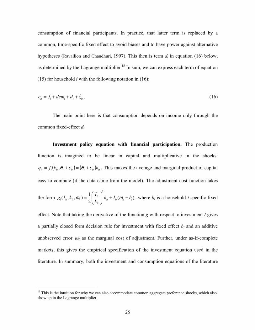
consumption of financial participants. In practice, that latter term is replaced by a

common, time-specific fixed effect to avoid biases and to have power against alternative

hypotheses (Ravallion and Chaudhuri, 1997). This then is term dt in equation (16) below,

as determined by the Lagrange multiplier.15 In sum, we can express each term of equation

(15) for household i with the following notation in (16):

ittiiit ddemfc ξ+++= . (16)

The main point here is that consumption depends on income only through the

common fixed-effect dt.

Investment policy equation with financial participation. The production

function is imagined to be linear in capital and multiplicative in the shocks:

( ) ( ) itittittitiit kkfq εθεθ +=+= , . This makes the average and marginal product of capital

easy to compute (if the data came from the model). The adjustment cost function takes

the form )(21),,(

2

iitititit

ititititi bIk

kIkIg ++⎟⎟⎠

⎞⎜⎜⎝

⎛= ωω , where bi is a household-i specific fixed

effect. Note that taking the derivative of the function g with respect to investment I gives

a partially closed form decision rule for investment with fixed effect bi and an additive

unobserved error ωit as the marginal cost of adjustment. Further, under as-if-complete

markets, this gives the empirical specification of the investment equation used in the

literature. In summary, both the investment and consumption equations of the literature

15 This is the intuition for why we can also accommodate common aggregate preference shocks, which also show up in the Lagrange multiplier.

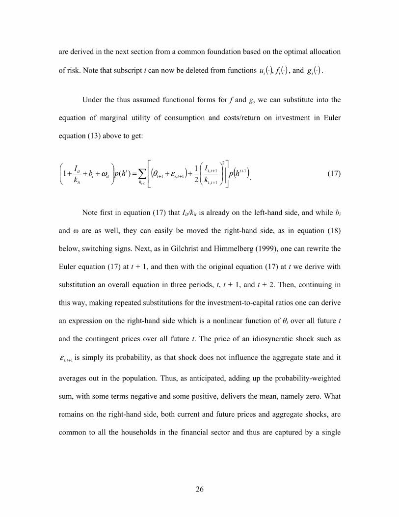
26

are derived in the next section from a common foundation based on the optimal allocation

of risk. Note that subscript i can now be deleted from functions ( ) ( )⋅⋅ ii fu , , and ( )⋅ig .

Under the thus assumed functional forms for f and g, we can substitute into the

equation of marginal utility of consumption and costs/return on investment in Euler

equation (13) above to get:

( ) ( )1

2

1,

1,1,1

121)(1 +

+

+++∑

+ ⎥⎥

⎦

⎤

⎢⎢

⎣

⎡

⎟⎟⎠

⎞⎜⎜⎝

⎛++=⎟⎟

⎠

⎞⎜⎜⎝

⎛+++ t

h ti

titit

titt

it

it hpkI

hpbkI

t

εθω .

(17)

Note first in equation (17) that Iit/kit is already on the left-hand side, and while bi

and ω are as well, they can easily be moved the right-hand side, as in equation (18)

below, switching signs. Next, as in Gilchrist and Himmelberg (1999), one can rewrite the

Euler equation (17) at t + 1, and then with the original equation (17) at t we derive with

substitution an overall equation in three periods, t, t + 1, and t + 2. Then, continuing in

this way, making repeated substitutions for the investment-to-capital ratios one can derive

an expression on the right-hand side which is a nonlinear function of θt over all future t

and the contingent prices over all future t. The price of an idiosyncratic shock such as

1, +tiε is simply its probability, as that shock does not influence the aggregate state and it

averages out in the population. Thus, as anticipated, adding up the probability-weighted

sum, with some terms negative and some positive, delivers the mean, namely zero. What

remains on the right-hand side, both current and future prices and aggregate shocks, are

common to all the households in the financial sector and thus are captured by a single

27

common time dummy. This is dt in equation (18) below.16 The main point is that

household investment depends on the aggregate fixed effect dt and not on household

income. The normalization with respect to kit gets rid of household specific technology

effects except for the marginal cost shifter ωit. Then, linearizing, again as in Gilchrist and

Himmelberg (1999):

ititit

it bdconstkI ω+++= 1 .

(18)

Consumption and investment equations under financial autarky. In the

autarky problem, consumption is determined at the same time as investment for

households running businesses, or at the same time as savings for wage earners, and so

consumption will be captured by similar equations to investment. The relevant state

variables are { }itittititk ωεθξ ,,, + and we write the policy functions as follows:

( )itittititiit kII ωεθξ ,,, += and ( )itittititiit kcc ωεθξ ,,, += . For wage earners, again replace k

with s and I with S. But again, we do not track savings the way we do for investment by

businesses, and so there are no investment equations to be estimated for wage earners.

The key point is that the current state for a household at the time of making the joint

consumption and investment (or savings) decision includes current income plus other

idiosyncratic shocks to preferences and adjustment costs. That is, for farms and business,

the state includes both the contemporaneous shocks θt + εit and also kit. Current income is

qit = kit (θt + εit), and as we have already included the contemporaneous shocks, the

16 This is related to dt in the consumption equation though not identical to it. We do not test the two equations jointly, so the distinction does not matter.

28

capital piece kit is the only thing otherwise left out of qit. With the linear approximation

we include each term separately.

In sum, the linear approximation of the policy functions for those in financial

autarky, replacing θt + εit by qit/kit are, for consumption

itit

ititit k

qkc χηη +⎟⎟⎠

⎞⎜⎜⎝

⎛+= 10 , (19)

where χit captures both ξit and ωit; and, for investment

itit

ititit k

qkI υφφ ~10 +⎟⎟

⎠

⎞⎜⎜⎝

⎛+= (20)

where itυ~ captures again both ξit and ωit. Now, as in equation (17) above for those in as-

if-complete markets, we normalize investment by the scale of the capital stock:

itit

it

it

it

it

kk

q

kI υφφ ~

10 +⎟⎟⎟

⎠

⎞

⎜⎜⎜

⎝

⎛

+= .

(21)

In this specification, with the error term now normalized by k, it is natural to check for

heteroskedasticity.

Impact equations of financial participation. Observed consumption and

investment at time t > 0 for those households i participating in the financial sector Pi0 = 1

and in financial autarky Pi0 = 0 can be written by using equations (16), (18), (19) and

(21):

29

[ ] ( ) ⎥⎦

⎤⎢⎣

⎡+⎟⎟⎠

⎞⎜⎜⎝

⎛+−++++= it

it

ititiittiiiit k

qkPddemfPc χηηξ 1000 1 (22)

[ ] ( )⎥⎥⎥

⎦

⎤

⎢⎢⎢

⎣

⎡

+⎟⎟⎟

⎠

⎞

⎜⎜⎜

⎝

⎛

+−++++= itit

it

it

iititiit

it

kk

q

PbdconstPkI νφφω 10010 1 .

(23)

By rearranging terms and taking first differences, and letting 1−−=Δ ttt ddd , we

rid ourselves of household-specific effects and get the following impact equations for

changes in consumption and investment-per-unit capital:

( )[ ]itiitiit

itiititiit PP

kqPkPdPc ξχηη Δ+Δ−+⎟⎟

⎠

⎞⎜⎜⎝

⎛Δ−+Δ−+Δ=Δ 0010000 1)1()1( (24)

[ ]itiitiit

it

it

itiit

it PvPk

kq

PdPkI ωφ Δ+Δ−+

⎟⎟⎟

⎠

⎞

⎜⎜⎜

⎝

⎛

Δ−+Δ=Δ 00100 )1()1( . (25)

If the idiosyncratic shock ξit is i.i.d., then the error terms in equations (24) and

(25) are i.i.d., and the participation decision Pio taken at t = 0 would be independent of

error terms in the impact equations, which implies in turn that the OLS estimates of

financial participation impact are unbiased. However, allowing serial correlation in the

idiosyncratic shock ξit will make OLS estimates biased and would require Instrumental

Variable (IV) estimation. Note that cost Zi does not affect potential levels of consumption

or investment other than in the initial date before our sample periods, but cost Zi does

affect the initial choice of financial participation. In this sense, Zi in the theory is a valid

30

instrument for the participation decision. The question is then what instrument we

employ in the data. IV estimation requires finding variables in the data that are correlated

with the cost of participation but uncorrelated with initial shocks ξi0, ωi0, θ0 and εi0.

Note that q / k appears in the consumption and investment equations for those

autarky households running firms and businesses, but not for wage earners who have no

k, only wage income. For empirical purposes we now put q / k in units of income for both

groups. That is, we run a simple linear regression of income onto q / k each year one at a

time for farms/businesses, and then use the rescaled predicted value. Note that this

income term is just a linear function of q / k. For wage earners we need not run a

regression and we just use reported income. This in first differences is “income change”,

one of the variables on the right-hand side of the consumption equation. The other term in

the consumption equation is capital change. We ran this specification and conducted

robustness checks with its exclusion. Results are not sensitive, so capital change is

dropped from results reported in Table 4 below. This also has the advantage of making

the autarky consumption equation more comparable to the empirical literature. The

investment equation is run only for farms and businesses and is already scaled by k so

there is no need to include k on the right-hand side. Finally, in earlier work (Alem and

Townsend 2004) we included demographic effects in levels and all interaction terms,

though this specification does not come from the theory. Results are largely similar.17

17 Specifically, control Xj96 is an expanded vector of household j characteristics including age, wealth, gender, and also other demographic terms (number of adult males, adult females and children). Control Zji96 is a vector of characteristics for village i of household j. From the Townsend Thai data we include average wealth of the village and average education. We also include measured CDD village characteristics such as fraction of households with piped water and state supplied electricity, number of households with migrants outside the village, whether there is a village assembly hall, fraction of households in agriculture, in cottage

31

Instruments. We employ several candidates as instruments for Zi and test them as

over-identifying restrictions (OIR) as we describe below. Each instrument has its strength

and limitations, and they all consist of alternative measures of the cost of financial

participation Zi based on geographic variation, as in Card (1995).18

Headman Response (HEAD): The key informant of a particular village in the

Townsend Thai survey answers retrospective questions delivering the history of

institution use, in particular the presence of a named institution in the base year, 1996.

That is, were there any households who were clients or used the services of a named

financial institution? This seems likely correlated with whether an individual is a member

or a customer, particularly so for institutions that operate at the village level only or

institutions that target or expand at the village level (less so for Commercial Banks, for

example). This instrument is not available for informal borrowing or savings.

Time to District Center (TIME): CDD data estimates travel times from the village

to District Centers. These are used as instruments for all formal institutions, though it is

questionable a priori if there is relevance in this for village institutions. Commercial

industries, in paddy production, and fraction receiving government assistance, and with multiple occupations. The Xj and Zji are all dated 1996 and all entered in both levels and interacted with income change. The goal is to have as many controls as possible for consumption and investment change to extract out the incremental smoothing effect of membership in an institution. 18 This strategy is vulnerable to the possibility that financial institutions choose where to operate based on the risk sharing capabilities of their borrowers. Though not implausible, there are indications of other motives in the data: Commercial banks cluster around towns as if a more aggressive strategy of lending to farmers or putting branches or mobile vans in rural areas were inconsistent with Bank of Thailand regulation. The BAAC tends over time to try to establish a branch in every county. Here we treat the placement as random, though clearly this at best an approximation, and focus on the choice of potential customers given branch location. It is clear from CDD data that households can travel non-trivial distances to get to somewhat distant branches. It is the cost of doing this that rationalizes several of the instruments we use. Ongoing work with Assuncao, Mityakov and Townsend (2010) is exploring these issues in detail but not enough is known at present to incorporate here.

32

banks might be supposed to operate near district centers, and the BAAC may target poor

farmers far off the main road.

Geographic Information System (GIS): We also created from CDD data another

instrument for financial participation that indicates institutional presence in 1996. Again,

Headmen of all villages in Thailand are asked in the CDD survey whether anyone in the

village has access to credit from each one of several named institutions such as village

funds, commercial banks, agricultural cooperatives, and traders or suppliers of inputs (as

a proxy for the informal sector). As all villages in each of the survey provinces have been

vectorized in a GIS, we can use the responses from nearby villages in 1996 to create a

weighted membership variable for each of the villages of the Townsend Thai survey.19

The GIS variable has several advantages. First, the response of any given headman may

be inaccurate, so with presumed spatial correlation, the averaging is removing some

measurement error. Second, we can impute values to villages that otherwise are missing

headmen responses. Third, there may be supply-side variation: For example, village

funds (PCG’s) are promoted by energetic local officials responsible for tambons or

amphoes.

The instruments we have chosen are by and large correlated with active

participation in the base year and subsequent use of the financial institutions, as shown in

Table 2. In many other applications with limited data, being a customer or member

19 Specifically every pixel is assigned a number by weighting the nearest 12 villages to the center of the pixel, the weight falling inversely with distance. Thus every village, including those of the Townsend Thai data, can be assigned an indicator. The weights and number of villages used were chosen to produce non-trivial variation, between zero and one, so that on average there is neither too little nor too much damping. Robustness checks with alternative specifications were performed.

33

cannot be checked directly with actual subsequent use, so here again a panel which asks

about savings and borrowing transactions by provider has its huge advantages.

(Insert Table 2 here)

Method. We use Instrumental Variables (IV) as the benchmark case but employ

Generalized Method of Moments (GMM) when the presence of heteroskedasticity in the

error term makes IV estimates of standard errors inconsistent. Assuming conditional

homoskedasticity, we calculate an IV estimator in two stages, test for the validity of sets

of instruments as over-identifying restrictions (OIR), and report the Sargan statistic. We

test for heteroskedasticity as in Pagan and Hall (1983), and when indicated, we use GMM

and report Hansen J-statistics for the validity of instruments. We first test for the validity

of the three instruments, and if this is rejected we test for the various combinations of

instruments pair-wise. The advantage of GMM in overcoming heteroskedasticity comes

with a cost, as Hayashi (2000) points out, which is that estimates of the optimal

weighting matrix require a very large sample size. We come back to this issue when we

report results.

Table 3 reports statistics on the relevance and validity of instruments employed on

each financial institution for both consumption and investment impact equations. The

first column presents the Shea (1997) partial R2 measure for (time) dummies interacted

with measured participation P0, and the second column the income coefficient interacted

with measured participation P0. Results indicate that the instruments are largely

correlated with these endogenous variables, which is what we expected. There are

exceptions. Note in particular that the partial correlation of instruments in the income

34

column for Agricultural Cooperatives and PCG in the consumption specification are low,

to anticipate future results. This is also true for Agriculture Cooperatives in the

investment specification. The third column reports the p-value of the Pagan-Hall (1983)

test for the presence of heteroskedasticity in the error term. It was found that the null

hypothesis of conditional homoskedasticity is not rejected for the consumption

specification, but it is uniformly rejected at 1% in the case of the investment equation.

The investment equation is thus estimated using the GMM instead of IV, and again we

anticipate weaker results. The last two columns report the p-value of the over-identifying

restrictions test, and we present in the last column the combination of instruments for

which the Sargan/Hansen statistic did not reject the null hypothesis of validity of

instruments.

(Insert Table 3 here)

7. The impact of financial institutions

Tables 4 and 5 present the estimates of consumption and investment impact

equations (24) and (25), respectively. The first column reports the point estimates (and p-

values) of the time-varying constant that measures consumption/investment co-

movements for members of the particular institution under analysis (BAAC, Commercial

Banks, Agricultural Cooperatives, PCG and the Informal Sector). The second column

reports the sensitivity of consumption/investment to income changes for non-participants

of the financial institution, and the third column measures the effect of financial

35

participation on the income coefficient sensitivity (that is, income change sensitivity for

members is the sum of the second and third columns). Finally, the last, fourth column,

tests the complete-markets-full-insurance hypothesis for financial participants.

(Insert Table 4 here)

Summary of results. The BAAC is the most helpful institution in the sense that it

helps both in consumption and investment. The sensitivity of consumption to income

changes is highest for those non-members of BAAC under IV estimation, but it is fully

undone for members in the IV specification, that is, members of the BAAC seem to enjoy

full insurance against income shocks (see the results in the last column). For investment,

both OLS and IV indicate that the BAAC has a favorable impact, though the impact of

the financial institution on the income coefficient (P0η1) subtracts too much and

consequently the complete markets hypothesis of the last column is rejected (at p-value

0.000). But see below for further discussion on this last point. The instruments employed

are correlated with subsequent use of both savings and credit (Table 2), though TIME has

a somewhat weaker correlation with subsequent use and is not a valid instrument in

consumption regression. Note that TIME has a positive correlation as more distant

customers are better served, consistent with the premise that BAAC customers are

usually located off road, so to speak.

(Insert Table 5 here)

What is the characteristic of the BAAC that allows this beneficial effect?

Townsend and Yaron (2001) examine this in a study of the BAAC risk contingency

36

system. When a farmer experiences an adverse shock during crop production, either

idiosyncratic illness which impedes farming, or an aggregate shock such as flood or

drought, then this is reported and verified if necessary by a BAAC field officer. The

BAAC can then extend the loan, and sometimes will forgive some of the (compound)

interest due and/or forgive some of the principal. The funds for this come from the central

government and are a line item in the BAAC accounts. In effect, the government is

paying a premium for insurance, while the farmers clearly receive an indemnity. The

point is that this de facto insurance arrangement is tailored around the farmers’ actual

situation and so a priori one might think that it would show up in consumption and

investment smoothing. Evidently this is the case.

Commercial banks are also helpful. In consumption smoothing, similar to the

BAAC, the impact of income changes on consumption is mitigated by financial

participation, again significant in the IV. For investment, the OLS specification indicates

a reduction in idiosyncratic risk, but that is not the case for the IV specification. It is

interesting that for commercial banks all three instruments (GIS, HEAD, TIME) are

valid, always. For commercial banks the correlation in Table 2 of the instrument Time to

District Center with subsequent use is negative, as one might anticipate, that is, nearby

customers are better served, so to speak. The negative sign on the instrument HEAD is a

puzzle.

For Agricultural Cooperatives and PCG/Village Funds it appears that customers

are as vulnerable as non-customers to shocks with respect to consumption. The sign is

negative for most specifications, but it is not statistically significant. With respect to

37

investment, the sign is perverse and significant in one case. These two institutions do not

appear helpful. Related perhaps, in Table 2, the correlation of the instruments with

subsequent use displays weak results for Agricultural Cooperatives.

The Informal Sector presents neutral if not perverse results with respect to the

smoothing of consumption from income shocks. Surprisingly, the favorable impact,

though overdone, is in investment (the F-test for complete markets is rejected), though

again see the discussion immediately following. Also, it seems it is the savings part (rice

storage), and not the informal borrowing part, which is picked up by the instruments

(TIME and GIS). Note the instrument TIME has a positive coefficient, as again more

distance from the district center means more use of rice storage.

As noted earlier, the coefficients in the IV regressions in investment for the

BAAC and the informal sector are negative and significantly different from zero, an odd

result. We have investigated this further. In the data used in this paper, the result for the

BAAC appears to be driven by low wealth households: if we drop the bottom 15% then

there is no net response to idiosyncratic risk, as the theory of full risk sharing implies,

i.e., full risk-sharing. In contrast, dropping high wealth households, different treatment of

outliers, and different treatment of zero investment events seem not to impact the result in

Table 5. The odd result for the informal sector and investment remains despite all these

robustness checks. However, results may be due to some kind of measurement error in

the annual data rather than anything substantive economically. In a different monthly data

set, but also for Thailand and these same provinces, Samphantharak and Townsend

(2009) do not find negative coefficients on either rich or poor households. Ongoing work

38

by Kinnan and Townsend (forthcoming) with that same monthly data find that the BAAC

and also commercial banks are helping in smoothing consumption (perfectly) and

investment (partially); further, there is no over-correction. Indeed, in the more detailed

monthly data where we know who is related to whom, and whether households give gifts

and transfers to each other, it seems indirect connections of a household to these formal

lenders can be quite helpful, either in smoothing along the equilibrium path, as for

consumption, or punishing off-equilibrium behavior, as for investment. These results are

preliminary, however.

8. Additional Results and Interpretation

As with the macro aggregates featured in the literature on the Asian financial crisis,

the first two years after the 1997 crisis correspond with drops in income and other key

variables, and the last year of the data corresponds with a recovery, especially so in the

Central Region. But despite the prevalence of aggregate shocks in income, consumption

and investment, idiosyncratic shocks abound. Part of this can be explained by

distinguishing income source and occupation group. For example, incomes did not drop

on average in these data for wage earners and those receiving remittances, unlike the

presumptions which underlay safety net targeting. Business on the other hand did suffer

income drops. Still, within each occupation category there remains considerable

idiosyncratic variation, evident in the histograms of income change. Thus an analysis of

the optimal allocation of risk is appropriate for these data.

The analysis of risk-sharing indicates there is little pattern by age and gender of the

household head, groups which are typically thought of as being in need of safety net

39

targeting. The least educated are more vulnerable, but there are exceptions. The most

salient finding is that wealth does matter, and the poor are uniformly more vulnerable in

both consumption and investment.

Stratifications by wealth and a frequency-of-use analysis with transactions data

seem to confirm a stereotypical picture of the literature: The poor lack access to formal

credit and insurance markets and are more reliant on remittances, moneylenders, and the

informal sector. They also seem more reliant on rice storage and livestock sales. The rich

have access to formal credit and use informal lending, savings in financial institutions,

and household and productive assets. However, when the transactions data are coupled

with the consumption, income, and investment data, a strikingly different pattern

emerges. Partial correlation coefficients of consumption-income deficits and investment-

income deficits with the various potential smoothing devices show that the poor segment

of the population are heavy users of formal credit, for both consumption and investment

smoothing. Informal borrowing is used more by the middle and upper wealth groups.

Likewise remittances, though used by all, seems relatively more important to the middle

and upper wealth groups. What remains of the stereotypical picture of the literature is that

the poor, and middle, segments are users of rice storage and the rich use savings in formal

institutions.

Stratifying by institution we find that the middle and upper classes by wealth do

seem to use commercial bank savings accounts to smooth consumption, running down

savings when there is a gap between consumption and income. Commercial bank lending

is available to few households. In contrast, we find in the transaction data that both

40

borrowing and saving with BAAC are helpful in consumption smoothing for the

relatively poor. This result helps us interpret the OLS and IV regressions. For example,

for village level quasi-formal financial institutions, we find in the transactions data that

movements in PCG credit and saving accounts do help smooth consumption, though only

for the rich, and smooth investment, but only for the middle group. An analysis of the

informal sector and the transactions data shows for consumption that informal borrowing

is helpful and significant under stratifications for the middle class only, not the poor.

Money lenders in particular serve the middle segment of the market. Regarding

investment, consistent with Tables 4 and 5, the transactions data show that informal

borrowing is helpful for the middle and rich, again with money lenders serving the

middle segment. Remittances help only the middle segment also. Storeowner credit helps

the rich (and to a lesser extent the poor, an exception). The conclusion again is that the

informal sector helps the wealthier groups. In contrast, here but not in Table 4, informal

savings in the form of buffer stocks is helpful in smoothing consumption for the poor and

middle wealth segments of the surveyed population.

9. Concluding Remarks

This paper presents a theory-based assessment of the impact of financial

institutions at the micro level, beyond financial statements and stand-alone financial

indicators. Access to financial institutions, as predicted from the theory, entails

substantial beneficial effects at the household level, particularly in eliminating the

damaging effect of income variability on consumption and investment. In particular, and

41

consistent with previous analysis (Townsend and Yaron 2001), government development

banks, usually considered culprits, seem to have a particularly beneficial effect. The more

general point is that theory and data can be combined to provide a rating of how well

financial service providers are doing as regards their actual customers and clients in the

provision of insurance. This link between the ratings of financial institutions and their

impact is rare. Certainly, the panel data required to do this is not typically available, but

on the other hand, the knowledge gained can be critical for regulators and policymakers

as they try to assess how well a given financial system is functioning and whether or not

there can be improvements.

42

References

Alem, M. and R.M. Townsend, 2004. An Evaluation of Safety Nets and Financial Institutions in

Crisis and Growth. Working paper, Dept. of Economics, University of Chicago.

Assuncao, J., S. Mityakov and R.M. Townsend, 2010. Bank Ownership and Expansion of the

Financial System in Thailand. Presentation made at AEA Annual Meetings, January 2,

2010, Atlanta.

Binford, M., T.J. Lee and R.M. Townsend, 2004. Sampling design for an integrated

socioeconomic and ecological survey by using satellite remote sensing and ordination.

Proceedings of the National Academy of Sciences, 101, 11517-11522.

Card, D., 1995. Using Geographic Variation in College Proximity to Estimate the Return to

Schooling, in: L.N. Christofides, E.K. Grant, and R. Swidinsky (Eds.), Aspects of Labor

Market Behaviour: Essays in Honour of John Vanderkamp. University of Toronto Press,

Toronto.

Gilchrist, S., and C. Himmelberg, 1999. Investment: Fundamentals and Finance, in: B. Bernanke,

and J. Rotemberg (Eds.), NBER Macroeconomics Annual 1998. MIT Press, Cambridge

and London.

Greenwood, J., and B. Jovanovic, 1990. Financial development, growth, and the distribution of

income. Journal of Political Economy, 98, 1076-1107.

Hayashi, F., 2000. Econometrics. Princeton University Press, Princeton, NJ.

43

Heckman, J.J. and E.J. Vytlacil, 2001. Local instrumental variables, in: C. Hsiao, K. Morimune,

and J.L. Powell (Eds.), Nonlinear Statistical Modeling: Proceedings of the Thirteenth

International Symposium in Economic Theory and Econometrics: Essays in Honor of

Takeshi Amemiya. Cambridge University Press, New York.

Jeong, H. and R.M. Townsend, 2008. Growth and Inequality: Model Evaluation Based on an

Estimation-Calibration Strategy. Macroeconomic Dynamics, 12, 231-84.

Kaboski, J,P., and R.M. Townsend, 2005. Policies and Impact: An Evaluation of Village-Level

Microfinance Institutions. Journal of the European Economic Association, 3, 1-50.

Kaboski, J.P., and R.M. Townsend, 2011. A Structural Evaluation of a Large-Scale Quasi-

Experimental Microfinance Initiative. Econometrica, 79, 1357-1406.

Kaboski, J.P., and R.M. Townsend, 2012. The Impact of Credit on Village Economies. American

Economic Journal: Applied Economics, 4, 1-38.

Kinnan, C. and R.M. Townsend, forth. Kinship and Financial Networks, Formal Financial Access

and Risk Reduction. Forthcoming in American Economic Review Papers and

Proceedings.

Pagan, A., and A.D. Hall, 1983. Diagnostic Tests as Residual Analysis. Econometric Reviews, 2,

59–218.

Puentes, E., 2009. Financial Deeping in Thailand. Unpublished project document, University of

Chile.

Ravallion, M., and S. Chaudhuri, 1997. Risk and Insurance in Village India: Comment.

Econometrica, 65, 171-184.

44

Samphantharak, K., and R.M. Townsend, 2009. Households as Corporate Firms: An Analysis of

Household Finance Using Integrated Household Surveys and Corporate Financial

Accounting. Cambridge University Press, Cambridge; New York.

Shea, J., 1997. Instrument Relevance in Multivariate Linear Models: A Simple Measure. Review

of Economics and Statistics, 79, 348-352.

Sripakdeevong, P. and R.M. Townsend, 2010. Informal Networks and Shadow Banking.

Unpublished project document, MIT.

Townsend, R.M., 1978. Intermediation with Costly Bilateral Exchange. Review of Economic

Studies, 45, 417-425.

Townsend, R.M., 1983. Forecasting the Forecasts of Others. Journal of Political Economy, 91,

546-587.

Townsend, R.M., 1994. Risk and Insurance in Village India. Econometrica, 62, 539-91.

Townsend, R.M., 1997. Townsend Thai Project Initial Institutional Survey, 1997.

http://hdl.handle.net/1902.1/10675 UNF:3:OHaCwbvWAvaqa3xrAMBFTA== Robert M.

Townsend; Murray Research Archive [Distributor] V1 [Version].

Townsend, R.M., and K. Ueda, 2006. Financial Deepening, Inequality, and Growth: A Model-

Based Quantitative Evaluation. Review of Economic Studies, 73, 251-93.

Townsend, R.M., and K. Ueda, 2010. Welfare Gains from Financial Liberalization. International

Economic Review, 51, 553-597.

45

Townsend, R.M., and S.S. Urzua, 2009. Measuring the Impact of Financial Intermediation:

Linking Contract Theory to Econometric Policy Evaluation. Macroeconomic Dynamics,

13, 268-316.

Townsend, R.M. and J. Yaron, 2001. The Credit Risk Contingency System of an Asian

Development Bank. Economic Perspectives, Third Quarter, Federal Reserve Bank of

Chicago, 25, 31-48.

Yaron, J., 1994. What Makes Rural Financial Institutions Successful? World Bank Research

Observer, 9, 49-70.

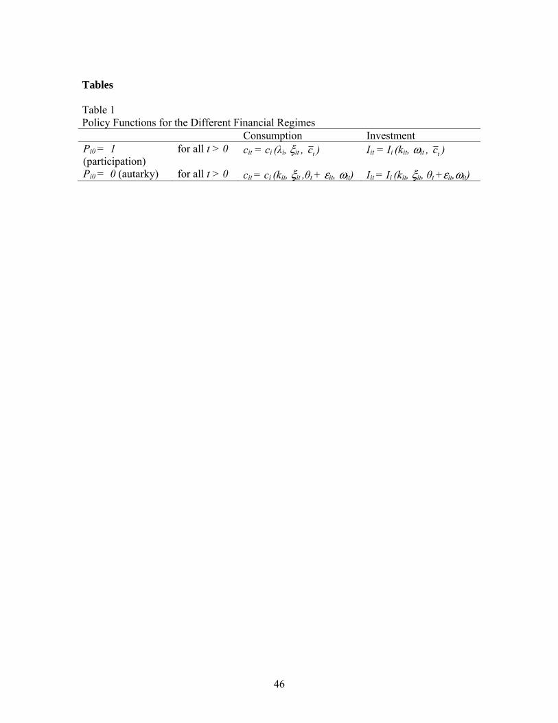
46

Tables Table 1 Policy Functions for the Different Financial Regimes Consumption Investment Pi0 = 1 (participation)

for all t > 0 cit = ci (λi, ξit , tc ) Iit = Ii (kit, ωit , tc )

Pi0 = 0 (autarky) for all t > 0 cit = ci (kit, ξit ,θt + εit, ωit) Iit = Ii (kit, ξit, θt +εit,ωit)

47

Table 2 Correlation of Instruments (listed in columns 2, 4, 6) with Frequency of Use HEAD P-value TIME P-value GIS P-valueBAAC - Borrowing .0869 (.0050) .0675 (.0307) .2115 (.0000)- Savings .0667 (.0313) .0602 (.0540) .2140 (.0000)Commercial Banks - Borrowing -.0209 (.4995) -.0795 (.0108) .0977 (.0016)- Savings .0558 (.0714) -.0988 (.0015) .0889 (.0041)Agric. Cooperatives - Borrowing .1062 (.0006) .0045 (.8847) .1818 (.0000)- Savings .1527 (.0000) -.0013 (.9678) .1897 (.0000)PCG - Borrowing .2186 (.0000) -.0961 (.0020) .1312 (.0000)- Savings .1943 (.0000) -.0930 (.0028) .1668 (.0000)Informal sector - Borrowing NA - .0174 (.5770) .0098 (.7522)- Savings (Rice) NA - .1228 (.0001) .0696 (.0244)Notes: GIS is the Geographical Information System instrument, TIME measures the travel time from the village to the district center and HEAD is the response of the Headman to questions about institutional presence. Frequent use is a dummy variable indicating whether the household had a transaction with named institution in 3 out of the 4 years in the panel. Note that informal sector borrowing is not highly correlated with the two available instruments.

48

Table 3 Properties of the Instruments Shea (1997) partial

R2 for endogenous variables

Pagan-Hall (1983) Test of

Heteroskedasticity

OIR test: Sargan/ Hansen

Combinations of instrument

P0 dt P0 q/k p-value p-value Consumption BAAC .994 .208 .675 .276 GIS,Head Comm. Banks .878 .424 .998 .668 GIS,Head,TimeAgric. Coop. .4160 .0121 .891 .2259 GIS,Time PCG .9056 .0984 .911 .1644 GIS,Time Informal sector .8747 .3306 .952 .6710 GIS,Time Investment BAAC .9922 .2300 .004 .8176 GIS,Head,TimeComm. Banks .8751 .2123 .000 .9158 GIS,Head,TimeAgric. Coop. .8403 .0628 .000 .5266 GIS,Head PCG .9273 .2223 .000 .7414 GIS,Head Informal sector .8984 .3615 .000 .4915 GIS,Time

49

Table 4 Impact of Financial Institutions on Consumption Smoothing (Eq. 24) F-test

P0 dt = 0 η1 P0 η1 F-test

η1+P0 η1= 0 (p-value) (p-value) (p-value) (p-value) BAAC OLS 1.66 .249*** -.062 13.04 (.157) (.000) (.439) (.000) IV 17.21 .571*** -.618*** .31 (.002) (.000) (.000) (.578) Commercial Banks OLS 8.01 .246*** -.094 7.97 (.000) (.000) (.234) (.0048) IV 29.58 .299*** -.223* 1.08 (.000) (.000) (.072) (.300) Agric. Cooperatives OLS 7.17 .204*** -.006 1.95 (.000) (.000) (.966) (.163) IV 34.25 .303*** -1.427 .77 (.000) (.010) (.304) (.379) PCG – Village Funds OLS 1.19 .221*** -.116 .33 (.313) (.000) (.539) (.567) IV 23.82 .196*** .427 1.31 (.000) (.000) (.455) (.253) Informal Sector OLS 4.45 .117*** .223*** 50.35 (.001) (.001) (.000) (.000) IV 32.70 .156*** .114 13.44 (.000) (.001) (.279) (.000)

50

Table 5 Impact of Financial Institutions on Investment Sensitivity to Shocks (Eq. 25) F-test

P0 dt = 0 φ 1 P0 φ1 F-test

φ1+P0 φ1= 0 (p-value) (p-value) (p-value) (p-value) BAAC OLS .76 .031*** -.192*** 77.19 (.5151) (.000) (.000) (.000) IV 3.54 .162*** -1.372*** 270.36 (.3150) (.000) (.000) (.000) Commercial Banks OLS .06 .010*** -.058* 2.26 (.983) (.002) (.066) (.133) IV 6.54 -.003 .026 .07 (.088) (.807) (.739) (.787) Agric. Cooperatives OLS .00 .010*** .381*** 9.32 (.999) (.002) (.003) (.002) IV 2.98 -.011 .436 .04 (.395) (.403) (.844) (.848) PCG – Village Funds OLS .03 .010*** .019 .01 (.994) (.002) (.956) (.932) IV 2.56 -.012 .966 .06 (.464) (.473) (.805) (.807) Informal Sector OLS 1.20 .030*** -.162*** 58.12 (.308) (.000) (.000) (.000) IV .02 .332*** -2.696*** 90.01 (.991) (.000) (.000) (.000)

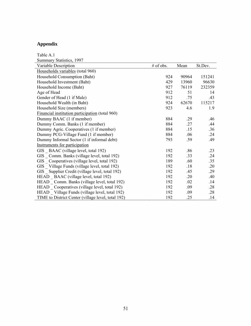
51

Appendix Table A.1 Summary Statistics, 1997 Variable Description # of obs. Mean St.Dev.Households variables (total 960) Household Consumption (Baht) 924 90964 151241Household Investment (Baht) 429 13960 96630Household Income (Baht) 927 76119 232359Age of Head 912 51 14Gender of Head (1 if Male) 912 .75 .43Household Wealth (in Baht) 924 62670 115217Household Size (members) 923 4.6 1.9Financial institution participation (total 960) Dummy BAAC (1 if member) 884 .29 .46Dummy Comm. Banks (1 if member) 884 .27 .44Dummy Agric. Cooperatives (1 if member) 884 .15 .36Dummy PCG-Village Fund (1 if member) 884 .06 .24Dummy Informal Sector (1 if informal debt) 793 .59 .49Instruments for participation GIS _ BAAC (village level, total 192) 192 .86 .23GIS _ Comm. Banks (village level, total 192) 192 .33 .24GIS _ Cooperatives (village level, total 192) 189 .60 .35GIS _ Village Funds (village level, total 192) 192 .18 .20GIS _ Supplier Credit (village level, total 192) 192 .45 .29HEAD _ BAAC (village level, total 192) 192 .20 .40HEAD _ Comm. Banks (village level, total 192) 192 .02 .14HEAD _ Cooperatives (village level, total 192) 192 .09 .28HEAD _ Village Funds (village level, total 192) 192 .09 .28TIME to District Center (village level, total 192) 192 .25 .14

52

Table A.2 Summary Statistics, panel data, 1998-2001 Variable Description # of obs. Mean St.Dev. Min. Max.Household variables (total 3840) Change in Consumption (Baht) 3682 -5183 46523 -154737 150106Change in Income (Baht) 3698 -8770 104747 -283033 147934Change in Investment/Capital (Baht) 2441 -.20 2.47 -12.08 6.46Capital - Level of Productive Assets (Baht) 3682 61359 78314 0 493790