An Evaluation of Combination Strategies for Test CaseSelection

Mats Grindal∗, Birgitta Lindstrom∗, Jeff Offutt†, and Sten F. Andler∗

2006-10-06

Abstract

This paper presents results from a comparative evaluation of five combination strategies. Com-bination strategies are test case selection methods that combine “interesting” values of the inputparameters of a test subject to form test cases. This research comparatively evaluated five com-bination strategies; the All Combination strategy (AC), the Each Choice strategy (EC), the BaseChoice strategy (BC), Orthogonal Arrays (OA) and the algorithm from the Automatic EfficientTest Generator (AETG). AC satisfies n-wise coverage, EC and BC satisfy 1-wise coverage, andOA and AETG satisfy pair-wise coverage. The All Combinations strategy was used as a “goldstandard” strategy; it subsumes the others but is usually too expensive for practical use. Theothers were used in an experiment that used five programs seeded with 128 faults.

The combination strategies were evaluated with respect to the number of test cases, the numberof faults found, failure size, and number of decisions covered.

The strategy that requires the least number of tests, Each Choice, found the smallest numberof faults. Although the Base Choice strategy requires fewer test cases than Orthogonal Arraysand AETG, it found as many faults. Analysis also shows some properties of the combinationstrategies that appear significant. The two most important results are that the Each Choicestrategy is unpredictable in terms of which faults will be revealed, possibly indicating that faultsare found by chance, and that the Base Choice and the pair-wise combination strategies to someextent target different types of faults.

Keywords: Combination Strategies, Orthogonal Arrays, AETG, Test Case Selection, TestingExperiment

∗School of Humanities and Informatics, University of Skovde, email: {mats.grindal,birgitta.lindstrom,sten.f.andler}@his.se†Department of Information and Software Engineering, George Mason University, Fairfax, VA 22030, USA, part-time

faculty researcher at the National Institute of Standards and Technology, email: offutt@ise.gmu.edu

1

1 Introduction

The input space of a test problem can be generally described by the parameters of the test subject 1.Often, the number of parameters and the possible values of each parameter result in too manycombinations to be useful. Combination strategies is a class of test case selection methods thatuse combinatorial strategies to select test sets that have reasonable size.

The combination strategy approach consists of two broad steps. In the first step, the testeranalyzes each parameter in isolation to identify a small set of “interesting” values for each pa-rameter. The term interesting may seem insufficiently precise and a little judgmental, but it iscommon in the literature. In order not to limit the use of combination strategies, this paper de-fines “interesting values” to be whatever values the tester decides to use. In the second step, thecombination strategy is used to select a subset of all combinations of the interesting values basedon some coverage criterion.

Some papers have discussed the effectiveness of combination strategies (Brownlie, Prowse &Phadke 1992, Cohen, Dalal, Fredman & Patton 1997, Kropp, Koopman & Siewiorek 1998). Thesepapers indicate the usefulness of combination strategies, but many questions still remain. Forinstance, few papers compare the different combination strategies. Thus, it is difficult to decidewhich combination strategy to use. This paper presents results from an experimental comparativeevaluation of five combination strategies.

Our previous paper surveyed over a dozen different combination strategies (Grindal, Offutt &Andler 2005). Five of these were chosen for this study. In this paper, a criterion is a rule forselecting combinations of values, and a strategy is a procedure for selecting values that satisfy acriterion.

The 1-wise coverage criterion requires each interesting value of each parameter to be representedat least once in the test suite. The Each Choice strategy satisfies 1-wise coverage directly byrequiring that each interesting value be used in at least one test case. The Base Choice strategysatisfies 1-wise coverage by having the tester declare a “base” value for each parameter, a basetest case that includes all base values, and then varies each parameter through the other values.

The pair-wise coverage criterion requires every possible pair of interesting values of any twoparameters be included in the test suite. The Orthogonal Arrays and Automatic Efficient TestGenerator strategies use different algorithms (described later) to satisfy pair-wise coverage.

The All Combinations strategy generates all possible combinations of interesting values of theinput parameters. Thus, AC subsumes all the other strategies and requires the most test cases. Itis considered to satisfy the n-wise criterion, where n is the number of parameters. AC is used as a“gold-standard” reference. It is usually too expensive for practical use, but provides a convenientreference for experimental comparison.

This paper evaluates and compares the combination strategies with respect to the number oftest cases, number of faults found, failure size, and number of decisions covered in an experimentcomprising five programs that were seeded with 128 faults.

Two joint combination strategies (BC+OA and BC+AETG) were created by taking the unionsof the respective test suites and these are also evaluated on the same grounds as the others.

1In testing the object being tested is often called “program under test” or “system under test.” However, since thispaper reports the results of an experiment, it uses the term test subject instead.

2

That is, the independent variable in the experiment is the selection strategy, and it has sevenvalues. There are four separate dependent variables, test cases, faults, decisions, and failure size.

The remainder of this paper presents our experimental procedure and results. Section 2 givesa more formal background to testing, test case selection methods, and how they are related to thecombination strategies evaluated in this work. Section 3 describes each combination strategy thatwas investigated. Section 4 contains the details of the experiments conducted, section 5 describesthe results of the experiment, and section 6 analyzes the results achieved. This analysis leads tothe formulation of some recommendations about which combination strategies to use. In section 7the work presented in this paper is contrasted with the work of others and future work is outlinedin section 8.

2 Background

Testing and other fault revealing activities are crucial to the success of a software project (Basili& Selby 1987). A fault in the general sense is the adjudged or hypothesized cause of an er-ror (Anderson, Avizienis, Carter, Costes, Christian, Koga, Kopetz, Lala, Laprie, Meyer, Randell& Robinson 1994). Further, an error is the part of the system state that is liable to lead to asubsequent failure (Anderson et al. 1994). Finally, a failure is a deviation of the delivered servicefrom fulfilling the system function.

These definitions are similar to typical definitions in empirical software testing research. Inparticular, the number of faults found is a common way to evaluate test case selection methods(Briand & Pfahl 1999, Ntafos 1984, Offutt, Xiong & Liu 1999, Zweben & Heym 1992). Thesedefinitions are also consistent with the definitions used in the paper that first described the testsubjects used in this experiment (Lott & Rombach 1996).

A test case selection method is a way to identify test cases according to a selection criterion.Most test case selection methods try to cover some aspect of the test subject, assuming thatcoverage will lead to fault detection. With different test case selection methods having differentcoverage criteria, an important question for both the practitioner and the researcher is: Given aspecific test problem, which test case selection methods should be used? In the general test problemsome properties of a software artefact should be tested to a sufficient level. Thus, the choice of testcase selection method depends on the properties that should be tested, the associated coveragecriteria of the test case selection method, and the types of faults that the test case selection methodtargets.

With focus on combination strategies, this research targets the question of finding a suitabletest case selection method to use.

A common view among researchers is that experimentation is a good way to advance the com-mon knowledge of software engineering (Lott & Rombach 1996, Harman, Hierons, Holocombe,Jones, Reid, Roper & Woodward 1999). For results to be useful it is important that the exper-iments are controlled and documented in such a way that the results can be reproduced (Basili,Shull & Lanubile 1999). Thus, a complete description of the work presented here can be found ina technical report (Grindal, Lindstrom, Offutt & Andler 2003).

3

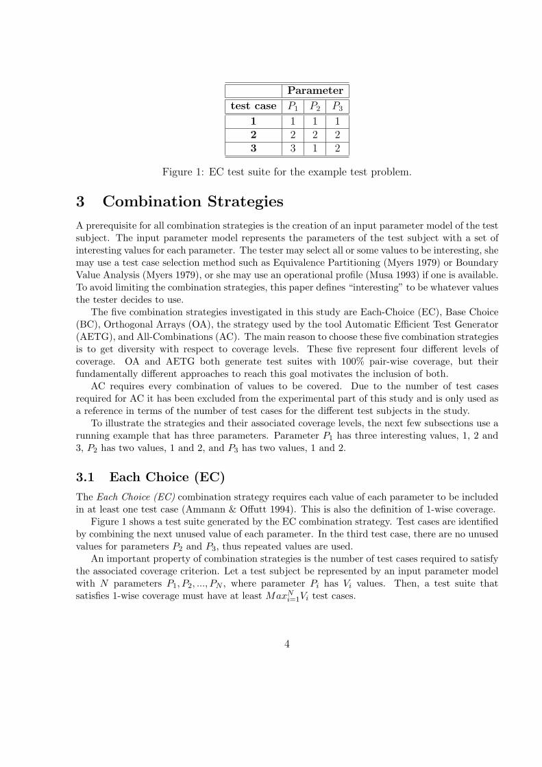
Parameter

test case P1 P2 P3

1 1 1 12 2 2 23 3 1 2

Figure 1: EC test suite for the example test problem.

3 Combination Strategies

A prerequisite for all combination strategies is the creation of an input parameter model of the testsubject. The input parameter model represents the parameters of the test subject with a set ofinteresting values for each parameter. The tester may select all or some values to be interesting, shemay use a test case selection method such as Equivalence Partitioning (Myers 1979) or BoundaryValue Analysis (Myers 1979), or she may use an operational profile (Musa 1993) if one is available.To avoid limiting the combination strategies, this paper defines “interesting” to be whatever valuesthe tester decides to use.

The five combination strategies investigated in this study are Each-Choice (EC), Base Choice(BC), Orthogonal Arrays (OA), the strategy used by the tool Automatic Efficient Test Generator(AETG), and All-Combinations (AC). The main reason to choose these five combination strategiesis to get diversity with respect to coverage levels. These five represent four different levels ofcoverage. OA and AETG both generate test suites with 100% pair-wise coverage, but theirfundamentally different approaches to reach this goal motivates the inclusion of both.

AC requires every combination of values to be covered. Due to the number of test casesrequired for AC it has been excluded from the experimental part of this study and is only used asa reference in terms of the number of test cases for the different test subjects in the study.

To illustrate the strategies and their associated coverage levels, the next few subsections use arunning example that has three parameters. Parameter P1 has three interesting values, 1, 2 and3, P2 has two values, 1 and 2, and P3 has two values, 1 and 2.

3.1 Each Choice (EC)

The Each Choice (EC) combination strategy requires each value of each parameter to be includedin at least one test case (Ammann & Offutt 1994). This is also the definition of 1-wise coverage.

Figure 1 shows a test suite generated by the EC combination strategy. Test cases are identifiedby combining the next unused value of each parameter. In the third test case, there are no unusedvalues for parameters P2 and P3, thus repeated values are used.

An important property of combination strategies is the number of test cases required to satisfythe associated coverage criterion. Let a test subject be represented by an input parameter modelwith N parameters P1, P2, ..., PN , where parameter Pi has Vi values. Then, a test suite thatsatisfies 1-wise coverage must have at least MaxN

i=1Vi test cases.

4

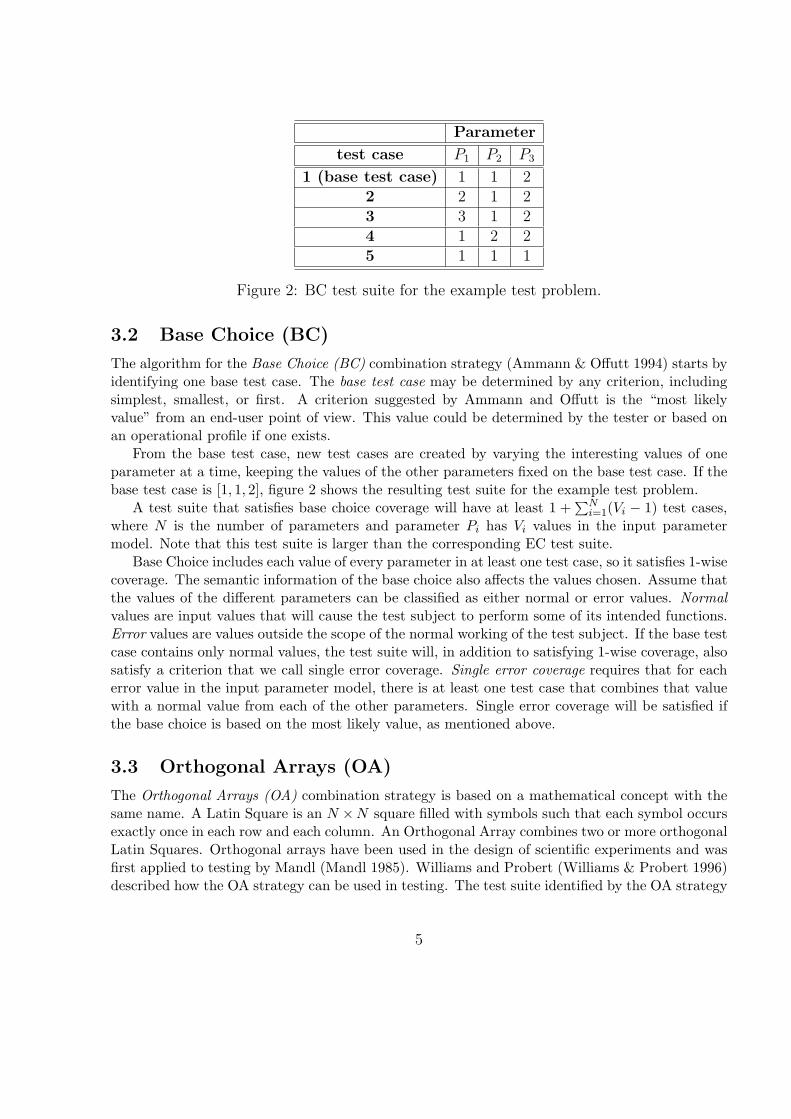
Parameter

test case P1 P2 P3

1 (base test case) 1 1 22 2 1 23 3 1 24 1 2 25 1 1 1

Figure 2: BC test suite for the example test problem.

3.2 Base Choice (BC)

The algorithm for the Base Choice (BC) combination strategy (Ammann & Offutt 1994) starts byidentifying one base test case. The base test case may be determined by any criterion, includingsimplest, smallest, or first. A criterion suggested by Ammann and Offutt is the “most likelyvalue” from an end-user point of view. This value could be determined by the tester or based onan operational profile if one exists.

From the base test case, new test cases are created by varying the interesting values of oneparameter at a time, keeping the values of the other parameters fixed on the base test case. If thebase test case is [1, 1, 2], figure 2 shows the resulting test suite for the example test problem.

A test suite that satisfies base choice coverage will have at least 1 +∑N

i=1(Vi − 1) test cases,where N is the number of parameters and parameter Pi has Vi values in the input parametermodel. Note that this test suite is larger than the corresponding EC test suite.

Base Choice includes each value of every parameter in at least one test case, so it satisfies 1-wisecoverage. The semantic information of the base choice also affects the values chosen. Assume thatthe values of the different parameters can be classified as either normal or error values. Normalvalues are input values that will cause the test subject to perform some of its intended functions.Error values are values outside the scope of the normal working of the test subject. If the base testcase contains only normal values, the test suite will, in addition to satisfying 1-wise coverage, alsosatisfy a criterion that we call single error coverage. Single error coverage requires that for eacherror value in the input parameter model, there is at least one test case that combines that valuewith a normal value from each of the other parameters. Single error coverage will be satisfied ifthe base choice is based on the most likely value, as mentioned above.

3.3 Orthogonal Arrays (OA)

The Orthogonal Arrays (OA) combination strategy is based on a mathematical concept with thesame name. A Latin Square is an N ×N square filled with symbols such that each symbol occursexactly once in each row and each column. An Orthogonal Array combines two or more orthogonalLatin Squares. Orthogonal arrays have been used in the design of scientific experiments and wasfirst applied to testing by Mandl (Mandl 1985). Williams and Probert (Williams & Probert 1996)described how the OA strategy can be used in testing. The test suite identified by the OA strategy

5

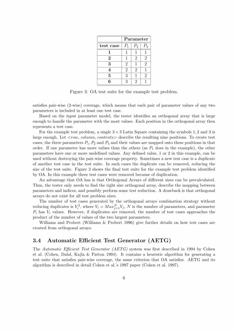
Parameter

test case P1 P2 P3

1 1 1 12 1 2 23 2 1 24 2 2 15 3 1 26 3 2 1

Figure 3: OA test suite for the example test problem.

satisfies pair-wise (2-wise) coverage, which means that each pair of parameter values of any twoparameters is included in at least one test case.

Based on the input parameter model, the tester identifies an orthogonal array that is largeenough to handle the parameter with the most values. Each position in the orthogonal array thenrepresents a test case.

For the example test problem, a single 3× 3 Latin Square containing the symbols 1, 2 and 3 islarge enough. Let <row, column, contents> describe the resulting nine positions. To create testcases, the three parameters P1, P2 and P3 and their values are mapped onto these positions in thatorder. If one parameter has more values than the others (as P1 does in the example), the otherparameters have one or more undefined values. Any defined value, 1 or 2 in this example, can beused without destroying the pair-wise coverage property. Sometimes a new test case is a duplicateof another test case in the test suite. In such cases the duplicate can be removed, reducing thesize of the test suite. Figure 3 shows the final test suite for the example test problem identifiedby OA. In this example three test cases were removed because of duplication.

An advantage that OA has is that Orthogonal Arrays of different sizes can be precalculated.Thus, the tester only needs to find the right size orthogonal array, describe the mapping betweenparameters and indices, and possibly perform some test reduction. A drawback is that orthogonalarrays do not exist for all test problem sizes.

The number of test cases generated by the orthogonal arrays combination strategy withoutreducing duplicates is V 2

i , where Vi = MaxNj=1Vj , N is the number of parameters, and parameter

Pi has Vi values. However, if duplicates are removed, the number of test cases approaches theproduct of the number of values of the two largest parameters.

Williams and Probert (Williams & Probert 1996) give further details on how test cases arecreated from orthogonal arrays.

3.4 Automatic Efficient Test Generator (AETG)

The Automatic Efficient Test Generator (AETG) system was first described in 1994 by Cohenet al. (Cohen, Dalal, Kajla & Patton 1994). It contains a heuristic algorithm for generating atest suite that satisfies pair-wise coverage, the same criterion that OA satisfies. AETG and itsalgorithm is described in detail Cohen et al.’s 1997 paper (Cohen et al. 1997).

6

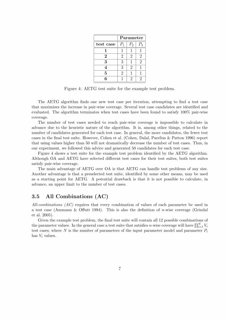
Parameter

test case P1 P2 P3

1 1 1 12 2 2 23 3 1 24 3 2 15 2 1 16 1 2 2

Figure 4: AETG test suite for the example test problem.

The AETG algorithm finds one new test case per iteration, attempting to find a test casethat maximizes the increase in pair-wise coverage. Several test case candidates are identified andevaluated. The algorithm terminates when test cases have been found to satisfy 100% pair-wisecoverage.

The number of test cases needed to reach pair-wise coverage is impossible to calculate inadvance due to the heuristic nature of the algorithm. It is, among other things, related to thenumber of candidates generated for each test case. In general, the more candidates, the fewer testcases in the final test suite. However, Cohen et al. (Cohen, Dalal, Parelius & Patton 1996) reportthat using values higher than 50 will not dramatically decrease the number of test cases. Thus, inour experiment, we followed this advice and generated 50 candidates for each test case.

Figure 4 shows a test suite for the example test problem identified by the AETG algorithm.Although OA and AETG have selected different test cases for their test suites, both test suitessatisfy pair-wise coverage.

The main advantage of AETG over OA is that AETG can handle test problems of any size.Another advantage is that a preselected test suite, identified by some other means, may be usedas a starting point for AETG. A potential drawback is that it is not possible to calculate, inadvance, an upper limit to the number of test cases.

3.5 All Combinations (AC)

All-combinations (AC) requires that every combination of values of each parameter be used ina test case (Ammann & Offutt 1994). This is also the definition of n-wise coverage (Grindalet al. 2005).

Given the example test problem, the final test suite will contain all 12 possible combinations ofthe parameter values. In the general case a test suite that satisfies n-wise coverage will have

∏Ni=1 Vi

test cases, where N is the number of parameters of the input parameter model and parameter Pi

has Vi values.

7

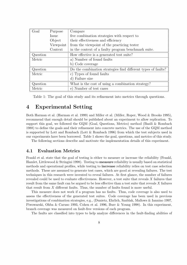
Goal Purpose CompareIssue five combination strategies with respect toObject their effectiveness and efficiencyViewpoint from the viewpoint of the practicing testerContext in the context of a faulty program benchmark suite.

Question How effective is a generated test suite?Metric a) Number of found faults

b) Code coverage

Question Do the combination strategies find different types of faults?Metric c) Types of found faults

d) Failure size

Question What is the cost of using a combination strategy?Metric e) Number of test cases

Table 1: The goal of this study and its refinement into metrics through questions.

4 Experimental Setting

Both Harman et al. (Harman et al. 1999) and Miller et al. (Miller, Roper, Wood & Brooks 1995),recommend that enough detail should be published about an experiment to allow replication. Tosupport this goal, we followed the GQM (Goal, Questions, Metrics) method (Basili & Rombach1988) to define the goals and their refinement into concrete metrics. The use of the GQM methodis supported by Lott and Rombach (Lott & Rombach 1996) from which the test subjects used inour experiments have been borrowed. Table 1 shows the goal, questions, and metrics of this study.

The following sections describe and motivate the implementation details of this experiment.

4.1 Evaluation Metrics

Frankl et al. state that the goal of testing is either to measure or increase the reliability (Frankl,Hamlet, Littlewood & Stringini 1998). Testing to measure reliability is usually based on statisticalmethods and operational profiles, while testing to increase reliability relies on test case selectionmethods. These are assumed to generate test cases, which are good at revealing failures. The testtechniques in this research were invented to reveal failures. At first glance, the number of failuresrevealed could be used to evaluate effectiveness. However, a test suite that reveals X failures thatresult from the same fault can be argued to be less effective than a test suite that reveals X failuresthat result from X different faults. Thus, the number of faults found is more useful.

This measure does not work if a program has no faults. Thus, code coverage is also used toassess the effectiveness of the generated test suites. Code coverage has been used in previousinvestigations of combination strategies, e.g., (Dunietz, Ehrlich, Szablak, Mallows & Iannino 1997,Piwowarski, Ohba & Caruso 1993, Cohen et al. 1996, Burr & Young 1998). In this experiment,branch coverage was measured on fault-free versions of each program.

The faults are classified into types to help analyze differences in the fault-finding abilities of

8

the combination strategies. Two classification schemes are used. The first is based on the numberof parameters involved in revealing the fault. The second is based on whether valid or invalidvalues are needed to reveal the fault.

During the analysis of the faults found by the different strategies, BC seemed to behave dif-ferently than the other strategies. The notion of failure size was introduced to understand thisbetter. Failure size is defined as the percentage of test cases in a test suite that fail for a specificfault. Failure size was inspired by the notion of fault size. Fault size is the percentage of inputsthat will trigger a fault, causing a failure (Bache 1997, Woodward & Al-Khanjari 2000, Offutt &Hayes 1996). In this experiment, the input parameter models are kept constant for all combinationstrategies, thus the fault sizes will be the same for all combination strategies.

In practice, the efficiency of a test selection method is related to the resources used, primar-ily time and money (Archibald 1992). Realistic resource consumption models of either of theseresources are difficult to both create and validate. Variation in the cost of computers, variationin human ability, and the increasing performance of computers are just some of the factors thatmake it difficult. Nevertheless, some researchers have used “normalized utilized person-time” as ameasure of the efficiency of a test case selection method (So, Cha, Shimeall & Kwon 2002).

This experiment uses a simplified model of resource consumption, in which the efficiency isapproximated with the number of test cases in each test suite. The motivation for this is that thesame input parameter models are used by all combination strategies. Further, it is assumed thatdifferences in time to generate the test suites are small compared to the time it takes to defineexpected results and execute the test cases.

4.2 Test Subjects

The main requirements on the test subjects are: (1) specifications for deriving test cases mustexist; (2) an implementation must exist; and (3) some known and documented faults must exist.

New test subjects can be created or already existing test subjects can be found. Creatingnew test subjects has the advantage of total control over the properties of the test subjects, e.g.,size, type of application, types of faults, source code language, etc. Drawbacks are that it takeslonger and creating programs in-house can introduce bias. A search on the Internet for existingtest subjects gave only one hit; the experimental package containing a “Repeatable SoftwareExperiment” including several different test objects by Kamsties and Lott (Lott n.d., Kamsties &Lott 1995b).

Using already existing test subjects also creates the possibility of cross-experiment comparisons(Basili et al. 1999). Thus, we used already existing test subjects.

The six programs were designed to be similar to Unix commands2 and initially used in an ex-periment that compared defect revealing mechanisms (Lott & Rombach 1996). This experimentalpackage was inspired by Basili and Selby (Basili & Selby 1987). The benchmark program suite hasbeen used in two independent experiments by Kamsties and Lott (Kamsties & Lott 1995a, Kam-sties & Lott 1995b), and later used in a replicated experiment by Wood et al. (Wood, Roper,Brooks & Miller 1997).

2The complete documentation of the Repeatable Software Experiment may be retrieved from URL: www.chris-lott.org/work/exp/.

9

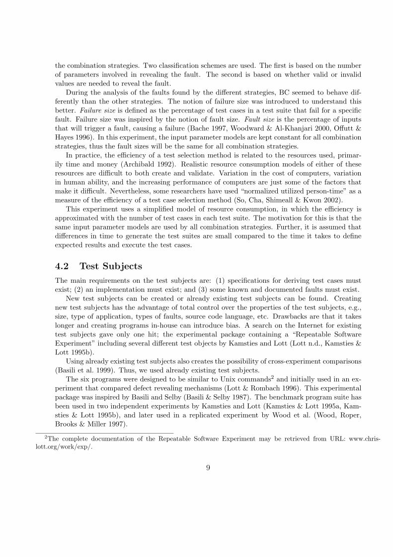
Test # Functions Lines # Decisions # Global NestingSubject of Code (a,c,f,i,w) Vars Levelcount 1 42 (0, 0, 0, 6, 2) 0 4tokens 5 117 (2, 1, 4, 12, 3) 4 3series 1 76 (0, 1, 1, 8, 0) 5 2nametbl 15 215 (4, 0, 0, 17, 0) 5 3ntree 9 193 (21, 0, 3, 10, 0) 0 3

Table 2: Descriptive size metrics of the programs. The number of decision points are divided into assert(’a’), case (’c’), for (’f’), if (’i’), and while (’w’) statements.

The programs are well documented, include specifications, and come with descriptions of ex-isting faults. We were able to use five of the six programs. The first, count, implements thestandard Unix command “wc.” count takes zero or more files as input and returns the number ofcharacters, words, and lines in the files. If no file is given as argument, count reads from standardinput. Words are assumed to be separated by one or more white-spaces (space, tab, or line break).

The second program, tokens, reads from the standard input, counts all alphanumeric tokens,and prints their counts in increasing lexicographic order. Several flags can be used to control whichtokens should be counted.

The third program, series, requires a start and an end argument and prints all real numbersbetween them in steps defined by an optional step size argument.

The fourth program, nametbl, reads commands from a file and runs one of several functionsbased on the command. Considered together, the functions implement a symbol table. For eachsymbol, the symbol table stores its name, the object type of the symbol, and the resource typeof the symbol. The commands let the user insert a new symbol, enter the object type, enter theresource type, search for a symbol, and print the entire symbol table.

The fifth program, ntree, also reads commands from a file and runs run one of several functionsbased on the command. The functions implement a tree in which each node can have any numberof child nodes. Each node in the tree contains a key and a content. The commands let the useradd a root, add a child, search for a node, check if two nodes are siblings, and print the tree.

The sixth program, cmdline, did not contain enough details in the specification to fit theexperimental set-up. Thus it was not used.

Table 2 contains some summary statistics of the five programs. All were implemented in theC programming language. We included main() in the number of functions. The counts of linesof code exclude any blank lines and lines that only contain comments. The number of decisionsincludes assert, case, for, if, and while statements. A case statement is counted as one decision.For global variables, each component of a struct is counted separately. Finally, the nesting levelis the highest nesting level for any function in the program.

10

4.3 Test Subject Parameters and Values

One of the most important conceptual tasks in using combination strategies is creating the inputparameter model. In their category partition method (Ostrand & Balcer 1988), Ostrand andBalcer discuss several approaches beyond the obvious idea of using the input parameters. Yin,Lebne-Dengel, and Malaiya (Yin, Lebne-Dengel & Malaiya 1997) suggest dividing the problemspace into sub-domains that can be thought of as consisting of orthogonal dimensions that do notnecessarily map one-to-one onto the actual input parameters of the implementation. Similarly,Cohen, Dalal, Parelius, and Patton (Cohen et al. 1996) suggest modeling the system’s functionalityinstead of its interface.

In this experiment, input parameter models were defined based on functionality represented by“abstract parameters”, such as the number of arguments, and how many of the same tokens areused. Equivalence partitioning (Myers 1979) was applied to these parameters and representativevalues were picked from each equivalence class. To support base choice testing, one equivalenceclass for each parameter was picked as the base choice class of that parameter. This made thecorresponding value the base value for that parameter. The values selected as base choices foreach parameter are all normal values.

Conflicts among parameters occur when some value of one parameter cannot be used with oneor more values of another parameter. An example of a conflict is when a value for one parameterrequires that all flags should be used, but values for another parameter states that a certain flagshould be turned off. AETG is the only strategy in this experiment that has built-in function tohandle conflicts. Ammann and Offutt (Ammann & Offutt 1994) suggested an outline for parameterconflict handling within BC that could also be used for EC. Williams and Probert (Williams &Probert 1996) suggested a way to handle parameter value conflicts within OA. However, Williamsand Probert’s method required the input parameter model to be changed. Since this would makecomparisons between the combination strategies less reliable, handling conflicts would introducea confounding variable into the experiment, thus all input parameter models were designed to beconflict free. If no complete conflict-free input parameter model could be designed, it was decidedthat some aspects of the test subject should be ignored to keep the input parameter model conflict-free, even at the cost of possibly loosing the ability to detect some faults. This was judged tobe more fair for this experiment. Obviously, in actual testing, parameter value conflicts mustbe handled, and ongoing studies include a closer look at different ways of handling parameterconflicts.

Tables 3 through 7 show the input parameter models for each test subject. As mentionedearlier, these models were influenced by the equivalence partitioning technique. To aid the reader,the tables contain both a description of the equivalence classes and the actual values selected fromeach class. The test case sets generated by the combination strategies are quite extensive and canbe found in an appendix in the technical report (Grindal et al. 2003).

4.4 Faults

The five programs in the study came with 33 known faults. The combination strategies exhibitedonly small differences in fault revealing for these faults, so an additional 118 faults were createdand seeded by hand. Most of these faults were mutation-like, such as changing operators in

11

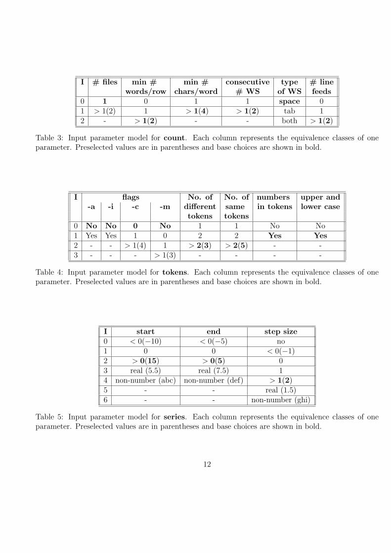
I # files min # min # consecutive type # linewords/row chars/word # WS of WS feeds

0 1 0 1 1 space 01 > 1(2) 1 > 1(4) > 1(2) tab 12 - > 1(2) - - both > 1(2)

Table 3: Input parameter model for count. Each column represents the equivalence classes of oneparameter. Preselected values are in parentheses and base choices are shown in bold.

I flags No. of No. of numbers upper and-a -i -c -m different same in tokens lower case

tokens tokens0 No No 0 No 1 1 No No1 Yes Yes 1 0 2 2 Yes Yes2 - - > 1(4) 1 > 2(3) > 2(5) - -3 - - - > 1(3) - - - -

Table 4: Input parameter model for tokens. Each column represents the equivalence classes of oneparameter. Preselected values are in parentheses and base choices are shown in bold.

I start end step size0 < 0(−10) < 0(−5) no1 0 0 < 0(−1)2 > 0(15) > 0(5) 03 real (5.5) real (7.5) 14 non-number (abc) non-number (def) > 1(2)5 - - real (1.5)6 - - non-number (ghi)

Table 5: Input parameter model for series. Each column represents the equivalence classes of oneparameter. Preselected values are in parentheses and base choices are shown in bold.

12

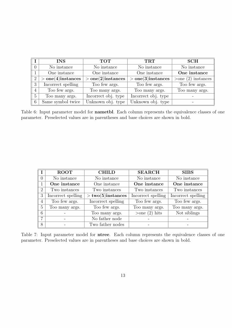
I INS TOT TRT SCH0 No instance No instance No instance No instance1 One instance One instance One instance One instance2 > one(4)instances > one(2)instances > one(3)instances >one (2) instances3 Incorrect spelling Too few args. Too few args. Too few args.4 Too few args. Too many args. Too many args. Too many args.5 Too many args. Incorrect obj. type Incorrect obj. type -6 Same symbol twice Unknown obj. type Unknown obj. type -

Table 6: Input parameter model for nametbl. Each column represents the equivalence classes of oneparameter. Preselected values are in parentheses and base choices are shown in bold.

I ROOT CHILD SEARCH SIBS0 No instance No instance No instance No instance1 One instance One instance One instance One instance2 Two instances Two instances Two instances Two instances3 Incorrect spelling > two(5)instances Incorrect spelling Incorrect spelling4 Too few args. Incorrect spelling Too few args. Too few args.5 Too many args. Too few args. Too many args. Too many args.6 - Too many args. >one (2) hits Not siblings7 - No father node - -8 - Two father nodes - -

Table 7: Input parameter model for ntree. Each column represents the equivalence classes of oneparameter. Preselected values are in parentheses and base choices are shown in bold.

13

'

&

$

%

Input

Parameter

Modeling

»»»»:

XXXXz

AbstractProblemDefinition(APD)

-

TestCaseMapping(TCM)

-

'

&

$

%

StrategySpecificSelection

-InputSpec.

(IS)¡¡¡ª

'

&

$

%

TestCaseFormatting

-TestSuite

(TS)¡¡¡ª

'

&

$

%

TestCaseExecution

-TestResults

LEGEND

FileFormat

Â

Á

¿

ÀTask

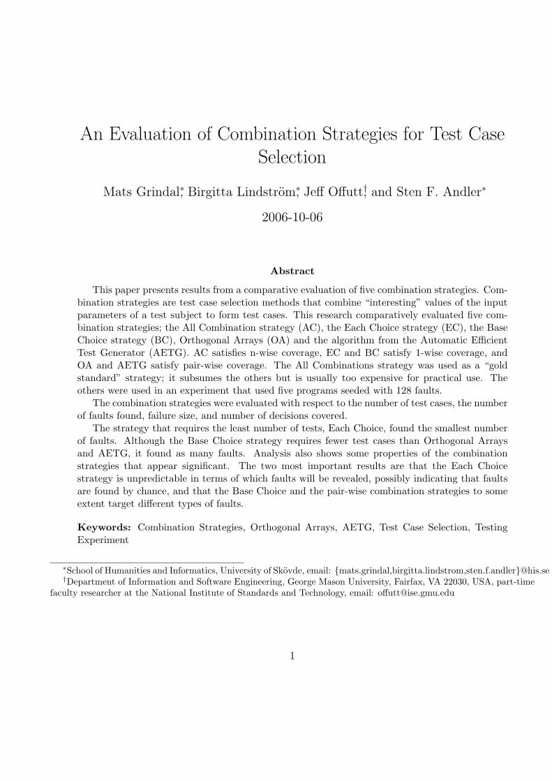
Figure 5: Test Case Generation and Execution

decisions, changing orders in enumerated types, and turning post-increment into pre-increment.Each function of every program contains at least one fault.

23 of the 151 faults were functionally equivalent to their original program. These were removedfrom the experiment, leaving a total of 128 faults.

Each fault was seeded in a separate copy of the program. This has the dual advantage ofavoiding interactions among the faults and making it obvious which fault is found when a failurehas occurred. This in turn made it easier to automate the experiment by using the Unix command“diff” to find the failures.

Next, simple instrumentation was added into the programs to measure code coverage. Faultswere not put into these extra statements and care was taken to ensure that they did not changethe programs’ functionalities. A complete description of the faults used in this study is given inthe technical report (Grindal et al. 2003).

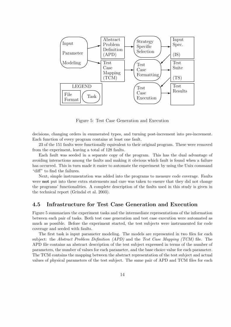
4.5 Infrastructure for Test Case Generation and Execution

Figure 5 summarizes the experiment tasks and the intermediate representations of the informationbetween each pair of tasks. Both test case generation and test case execution were automated asmuch as possible. Before the experiment started, the test subjects were instrumented for codecoverage and seeded with faults.

The first task is input parameter modeling. The models are represented in two files for eachsubject: the Abstract Problem Definition (APD) and the Test Case Mapping (TCM) file. TheAPD file contains an abstract description of the test subject expressed in terms of the number ofparameters, the number of values for each parameter, and the base choice value for each parameter.The TCM contains the mapping between the abstract representation of the test subject and actualvalues of physical parameters of the test subject. The same pair of APD and TCM files for each

14

test subject were used for all combination strategies. The formats of these files are given in detailin the technical report (Grindal et al. 2003).

The second task is generation of abstract test cases. Based on the contents of the APD file,each combination strategy generates a separate abstract test suite called Input Specification (IS).It contains a list of test cases represented as tuples of parameter values. The test suites weregenerated automatically, except for OA, whose tests were created manually because it was deemedeasier than implementing the OA algorithm.

The third task is translating abstract test cases to real inputs. The abstract test cases fromthe IS files were automatically converted into executable test cases by using the contents of theTCM file. For every parameter, the appropriate value in the TCM file was located by using theparameter name and value as index. The values identified by the different parameter values of atest case were appended to form the test case inputs. The actual test cases were stored in the TestSuite (TS) file.

The final task is to execute the test cases. A Perl script test case executor took the TS file asinput and executed each test case in the file. The test case executor also created a log file in whichthe names of the different test cases are logged together with any response from the test subject.This log was compared with a reference log created by executing the test suite on a correct versionof the program using the Unix “diff.”

4.6 Threats to Validity

Lack of independence is a common threat to validity when conducting an experiment. Our ap-proach was to introduce as much independence as possible throughout the experiment. We usedan externally developed suite of test subjects. The additional faults were created by a person(third author) not previously involved in the experiment. To further avoid bias, an algorithm wasfollowed for seeding faults as mutation-like modifications. Also, the five input parameters modelswere created without any knowledge of either the existing faults or the implementations. In factall the test cases were generated prior to studying the faults and the implementations. These stepsavoided all anticipated bias from lack of independence.

An obstacle in any software experiment is how representative the subjects are. In this ex-periment this issue applies to both programs and faults. A necessary condition in deciding if asample is representative is knowledge about the complete population. Unfortunately, we do notunderstand the populations of either programs or faults. This is a general problem in softwareexperimentation, not only for this study. This obviously limits the conclusions that can be drawn,therefore limiting external validity. Reasoning about the ability to detect different types of faultsinstead of just how many can help with this problem. Also, replicating experiments with differentsubjects is necessary.

Another aspect of representativity is whether a tester is likely to use the test strategies onthis type of test object. As described in section 3, combination strategies are used to identifytest cases by combining values of the test subject input parameters. This property makes combi-nation strategies suitable for test problems that have discrete value inputs. However, the testercan always sample a continuous parameter, which is a fundamental aspect of equivalence parti-tioning, boundary value analysis, and many other test methods. Thus, we draw the conclusion

15

that combination strategies are applicable to any test problem that can be expressed as a set ofparameters with values that should be combined to form complete inputs, which is the case for alltest subjects in this study.

The decision to avoid conflicts between values of different parameters in the input parametermodel could also raise a threat to validity. This decision made it impossible to detect three faults.However, all test techniques used the same input parameter models, so this decision affected alltechniques equally. That is, none of the test techniques could detect these three faults.

The process of making an input parameter model has much in common with equivalencepartitioning in the sense that one value may be selected to represent a whole group of values. Theunderlying assumption is that all values in an equivalence class will detect a fault equally well.The accuracy of this assumption depends both on the faults we actually have and the experienceof the tester. Different testers are likely to derive different classes. Hence, it is desirable to definethe equivalence classes in such way that they are representative both with respect to faults andtesters. We consider this particular form of representativity very hard to validate. Again, thisaffected all test techniques equally, so we believe that this only poses a minor threat to the validityof this experiment.

A more in-depth discussion of the validity issues in general may be found in our workshoppaper (Lindstrom, Grindal & Offutt 2004).

5 Results

This section presents results from the experiment. First the number of test cases is presented,then the number and types of faults found, the decision coverage, and finally the failure sizes.

An initial observation from this experiment was that BC and the pair-wise combination strate-gies (OA and AETG) target different types of faults. Thus, a logical course of action is toinvestigate the results of combining BC with either OA or AETG. Results for (BC+OA) and(BC+AETG) are included in the data. These results have been derived from the individual re-sults by taking the unions of the test suites of the included combination strategies, eliminatingduplicates.

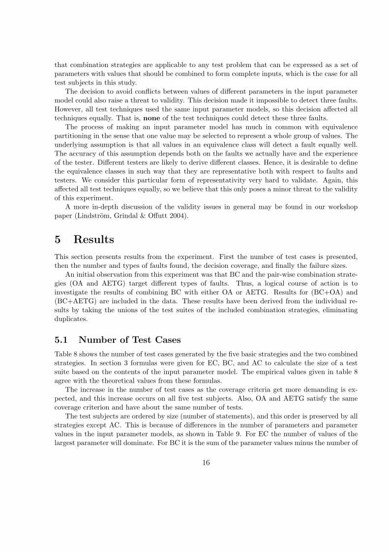
5.1 Number of Test Cases

Table 8 shows the number of test cases generated by the five basic strategies and the two combinedstrategies. In section 3 formulas were given for EC, BC, and AC to calculate the size of a testsuite based on the contents of the input parameter model. The empirical values given in table 8agree with the theoretical values from these formulas.

The increase in the number of test cases as the coverage criteria get more demanding is ex-pected, and this increase occurs on all five test subjects. Also, OA and AETG satisfy the samecoverage criterion and have about the same number of tests.

The test subjects are ordered by size (number of statements), and this order is preserved by allstrategies except AC. This is because of differences in the number of parameters and parametervalues in the input parameter models, as shown in Table 9. For EC the number of values of thelargest parameter will dominate. For BC it is the sum of the parameter values minus the number of

16

Combination StrategyTest Subject EC BC OA AETG BC+OA BC+AETG ACcount 3 10 14 12 23 21 216tokens 4 14 22 16 35 29 1728series 7 15 35 35 48 48 175nametbl 7 23 49 54 71 76 1715ntree 9 26 71 64 93 89 2646

total 30 88 191 181 270 263 6480

Table 8: Number of test cases generated by the combination strategies.

Test Subject # Parameters # Values for Total Valueseach Parameter

count 6 2, 3, 2, 2, 3, 3 15tokens 8 2, 2, 3, 4, 3, 3, 2, 2 21series 3 5, 5, 7 17nametbl 4 7, 7, 7, 5 26ntree 4 6, 9, 7, 7 29

Table 9: Sizes of test subjects.

parameters that gives the approximate number of test cases. For both OA and AETG the productof the number of values of the two largest parameters gives an approximate size of the test suite.Even if duplicates are removed for the two combined strategies, the order is still preserved whentaking the unions of the included test suites. Finally, for AC, the number of test cases is theproduct of the number of values of each parameter. A test subject with many parameters withfew values will require more test cases than a test subject with few parameters with many valueseven if the total number of values are the same. This can be seen in the case of tokens.

The large numbers of tests for AC effectively demonstrates why it is usually not consideredpractical.

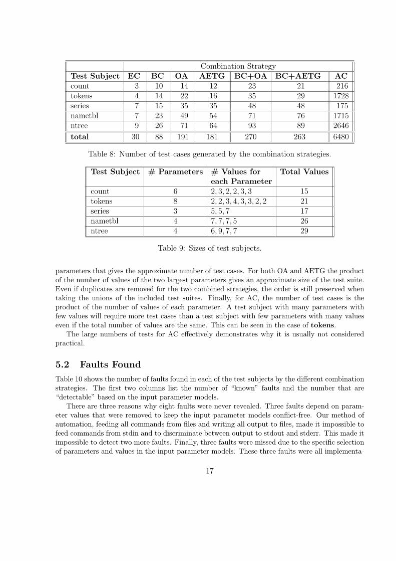
5.2 Faults Found

Table 10 shows the number of faults found in each of the test subjects by the different combinationstrategies. The first two columns list the number of “known” faults and the number that are“detectable” based on the input parameter models.

There are three reasons why eight faults were never revealed. Three faults depend on param-eter values that were removed to keep the input parameter models conflict-free. Our method ofautomation, feeding all commands from files and writing all output to files, made it impossible tofeed commands from stdin and to discriminate between output to stdout and stderr. This made itimpossible to detect two more faults. Finally, three faults were missed due to the specific selectionof parameters and values in the input parameter models. These three faults were all implementa-

17

Test Subject Faults Combination Strategyknown detectable EC BC OA AETG BC+OA BC+AETG

count 15 12 11 12 12 12 12 12tokens 15 11 11 11 11 11 11 11series 20 19 14 18 19 19 19 19nametbl 49 49 46 49 49 49 49 49ntree 29 29 25 29 26 26 29 29

total 128 120 107 119 117 117 120 120% of detectable 89 99 98 98 100 100

Table 10: Number of faults revealed by the combination strategies.

Test Subject t-factor0 1 2 3 4+

count 2 7 3 0 0tokens 3 4 4 0 0series 0 3 4 12 0nametbl 2 16 30 1 0ntree 0 8 9 12 0

total 7 38 50 25 0

Table 11: Number of t-factor faults in each test subject with respect to the input parameter modelsused in this study.

tion specific. One example of this is a function in the series program to handle rounding errors inthe conversion between real and integers. Reals within a 10−10 area of an integer are consideredequal. To detect the fault in this function a real value within the rounding area would have beenneeded, but since this was not defined in the specification no such value was used.

Dalal and Mallows (Dalal & Mallows 1998) give a model for software faults in which faults areclassified according to how many parameters (factors) need distinct values to cause the fault toresult in a failure. A t-factor fault is triggered if the values of t parameters are required to triggerit. This model is used to analyze the faults in this study. Table 11 shows the number of t-factorfaults for each test subject with respect to its input parameter model. A 0-factor fault is revealedby any combination of parameter values.

The number of t-factor faults for each t is a direct consequence of the contents of the inputparameter model. A changed input parameter model may affect the t-factor classification of faults.

A few of the faults turned out to be 0-factor faults. These are faults that will always produce afailure with the input parameter models used in this experiment. Another interesting observationis that there are no 4+-factor faults and only 25 3-factor faults of the total 120 faults. Thesame observation, that is, that most faults are 2-factor or less and thus detectable with pair-wisestrategies, has been made in a real industry setting. In a study of medical device software, Wallace

18

and Kuhn report that 98% of the faults are 2-factor or less (Wallace & Kuhn 2001). These resultsmay or may not generalize to other kinds of software and actual faults, so additional studies aredesirable.

It may be surprising that EC reveals 89% of the detectable faults even though it had relativelyfew test cases. The 0-factor faults will always be revealed and by definition, EC also guaranteesdetection of all 1-factor. Taken together, these account for slightly more than one third of thedetectable faults.

Many of the 2+-factor faults in this study share the property that many different combinationsof values of the involved parameters result in failure detection. Only a small group of the 2+-factor faults require exactly one combination of values of the involved parameters to be revealed.Obviously, the faults revealed by many combinations have a higher chance of being detected thanfaults revealed by only one combination. Cohen et al. (Cohen et al. 1994) claims that the samesituation, that is, that a large number of faults may be revealed by many different parametercombinations, is true for many real-world systems. This is probably why EC is so effective in thisstudy. However, it should be stressed that even if a 2+-factor fault has a high detection rate dueto many combinations revealing that fault, EC cannot be guaranteed to detect it.

It is not surprising that BC revealed more faults than EC; after all, it requires more tests. Butit may be surprising that BC found a similar number of faults (even slightly more) than OA andAETG, both of which require more tests and more combinations of choices. Looking in detail atthe faults is illuminating.

The only fault that BC missed was revealed by EC and both OA and AETG. This fault islocated in the series program and is a 3-factor fault. Parameter one has five possible values,parameter two also has five possible values, and parameter three has seven possible values, givinga total of 175 possible combinations. Exactly six of these combinations will trigger this fault.Parameter one and two both need to have one specific value and parameter three can have anyvalue except the value 1. None of the values of parameters one and two are base choices, whichexplains why BC not only missed this fault, but also could not reveal it. That is, revealing thisfault required two non-base choice values.

OA and AETG both satisfy pair-wise coverage – every combination of values of two parametersis included in the test suites. In the case of the fault missed by BC, the specific combination ofvalues of parameter one and two is included in one test case in each test suite. However, it is notenough for this combination to reveal the fault, so there is no guarantee that OA or AETG willreveal the fault. But since the third parameter may have several different values and still triggerthe fault, the chance of OA and AETG selecting a fault revealing combination is relatively high.This is why EC is so effective, as explained earlier. The chance of EC revealing this fault is small(6 chances out of 175, 3.4%), and the fact that EC revealed it seems largely due to chance. Onthe other hand, pair-wise strategies have 6 chances out of 7 of revealing the fault (87%) so it isnot surprising that OA and AETG found it.

The three faults that only BC revealed are all located in the ntree program. Its input param-eter model contains four parameters with six, nine, seven, and seven values respectively.

The first fault requires two of the parameters to have one specific value each, one, whichhappened to be a base choice and a third parameter to have any normal value. Both OA andAETG had one test case each in their test suite with the specific combination of the two parameters,

19

Combination StrategyTest Subject EC BC OA AETGcount 83 83 83 83tokens 82 82 86 86series 90 90 95 95nametbl 100 100 100 100ntree 83 88 88 88

Table 12: Percent decision coverage achieved for the correct versions of the test subjects.

but in both cases the third parameter happened to be invalid, so these two strategies did not revealthis fault. This is a good example of fault masking by an invalid value. BC revealed this faultbecause one of the parameters required exactly the base choice value and the third parameterrequired any normal value, including the base choice, which is satisfied by the base choice.

The second and third faults that were only revealed by BC are located in the same line ofcode, and both faults fail for the same combinations of parameter values. For these faults to betriggered, three parameters need to have one specific value each. This means that neither EC,OA, nor AETG can guarantee detection. However, two of the three required parameter valueshappened to be base choices, so BC was guaranteed to reveal this fault under this input parametermodel.

OA and AETG revealed exactly the same faults. Thus we can expect combining either withBC to yield the same results. In this experiment both combinations revealed all detectable faults.

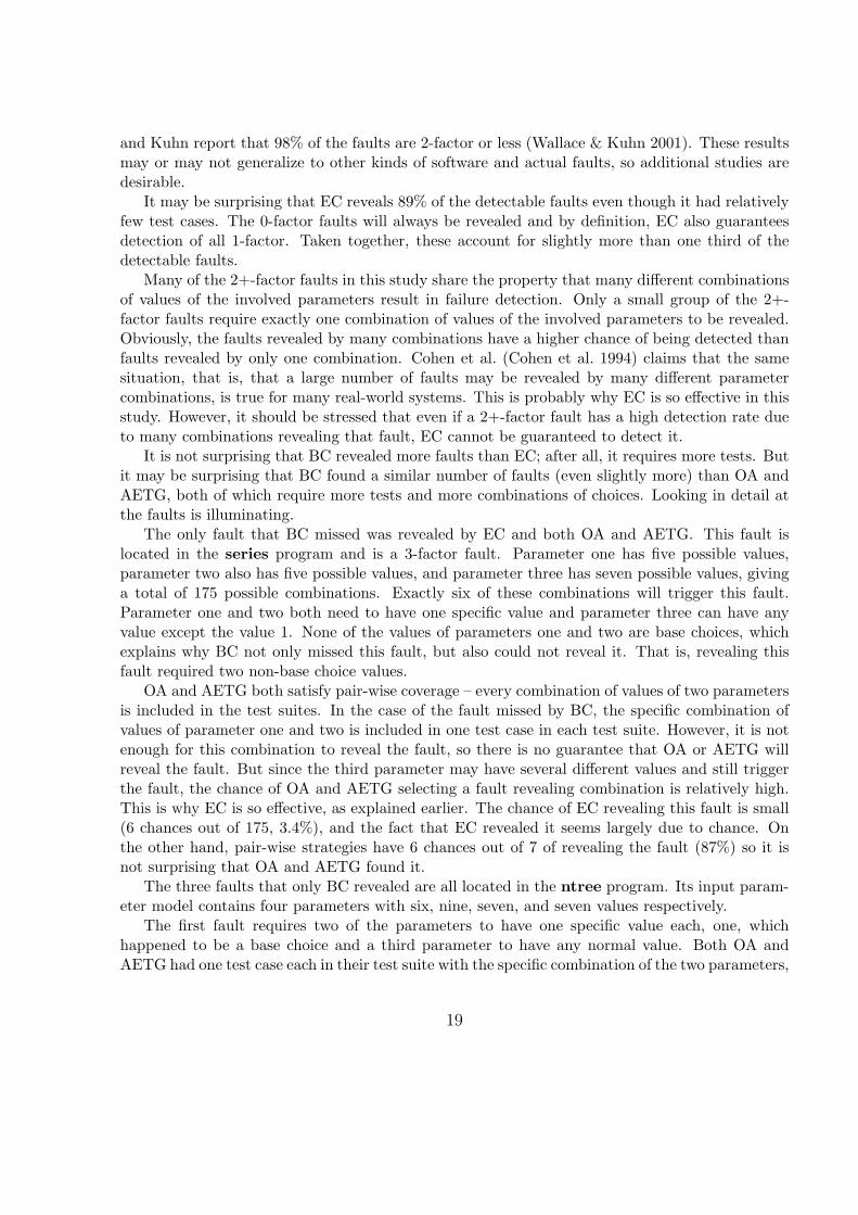
5.3 Decision Coverage

Table 12 shows the decision coverage achieved by each combination strategy on the correct versionsof the test subjects. Very little difference was found. OA and AETG covered slightly more decisionoutcomes than EC did, which can be expected since they had more tests.

These data are also similar to data from previous studies. Cohen, Dalal, Parelius, andPatton (Cohen et al. 1996) obtained over 90% block coverage and Burr and Young (Burr &Young 1998) reached 93% block coverage in experiments using AETG.

It was a little surprising that EC covered as many decisions as it did. As was shown in table 2the test subjects were all relatively small, in particular with respect to the number of decisionpoints, which means that there is a fair chance of reaching relatively high code coverage even withfew test cases.

The high decision coverage achieved for all test subjects by the EC test suites seems to indicatethat for this experiment:

1. There is a close correspondence between the specifications and the implementations of thetest subjects.

2. The selected parameters and parameter values used for testing the test subjects are goodrepresentatives of the total input space.

20

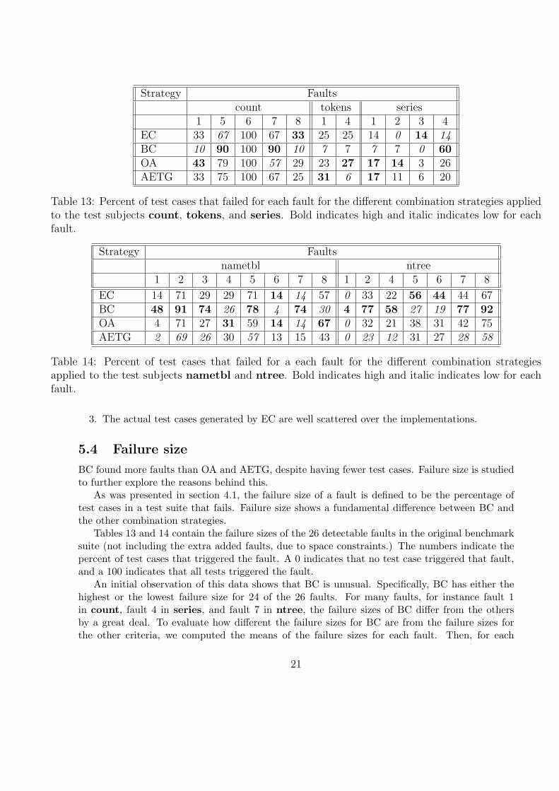
Strategy Faultscount tokens series

1 5 6 7 8 1 4 1 2 3 4EC 33 67 100 67 33 25 25 14 0 14 14BC 10 90 100 90 10 7 7 7 7 0 60OA 43 79 100 57 29 23 27 17 14 3 26AETG 33 75 100 67 25 31 6 17 11 6 20

Table 13: Percent of test cases that failed for each fault for the different combination strategies appliedto the test subjects count, tokens, and series. Bold indicates high and italic indicates low for eachfault.

Strategy Faultsnametbl ntree

1 2 3 4 5 6 7 8 1 2 4 5 6 7 8

EC 14 71 29 29 71 14 14 57 0 33 22 56 44 44 67BC 48 91 74 26 78 4 74 30 4 77 58 27 19 77 92OA 4 71 27 31 59 14 14 67 0 32 21 38 31 42 75AETG 2 69 26 30 57 13 15 43 0 23 12 31 27 28 58

Table 14: Percent of test cases that failed for a each fault for the different combination strategiesapplied to the test subjects nametbl and ntree. Bold indicates high and italic indicates low for eachfault.

3. The actual test cases generated by EC are well scattered over the implementations.

5.4 Failure size

BC found more faults than OA and AETG, despite having fewer test cases. Failure size is studiedto further explore the reasons behind this.

As was presented in section 4.1, the failure size of a fault is defined to be the percentage oftest cases in a test suite that fails. Failure size shows a fundamental difference between BC andthe other combination strategies.

Tables 13 and 14 contain the failure sizes of the 26 detectable faults in the original benchmarksuite (not including the extra added faults, due to space constraints.) The numbers indicate thepercent of test cases that triggered the fault. A 0 indicates that no test case triggered that fault,and a 100 indicates that all tests triggered the fault.

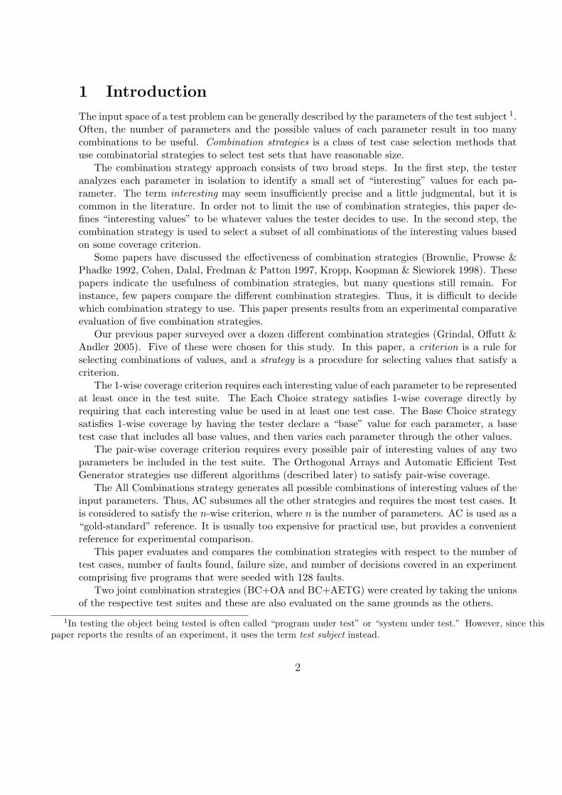
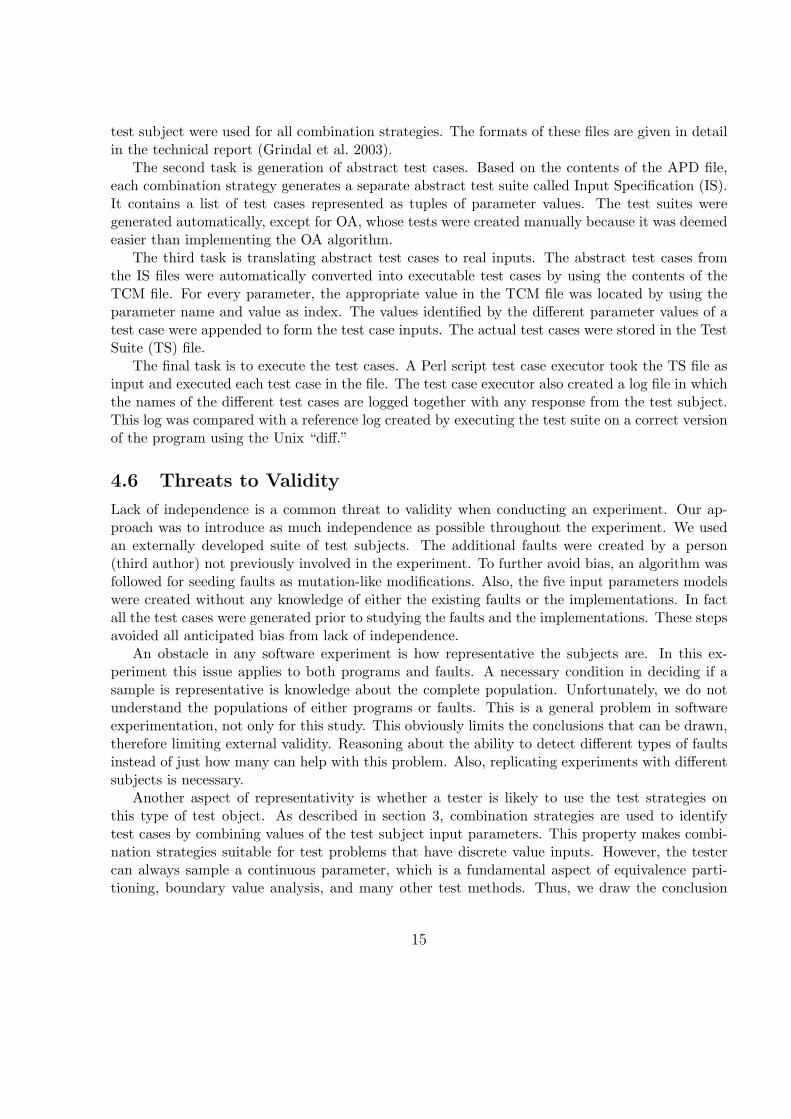
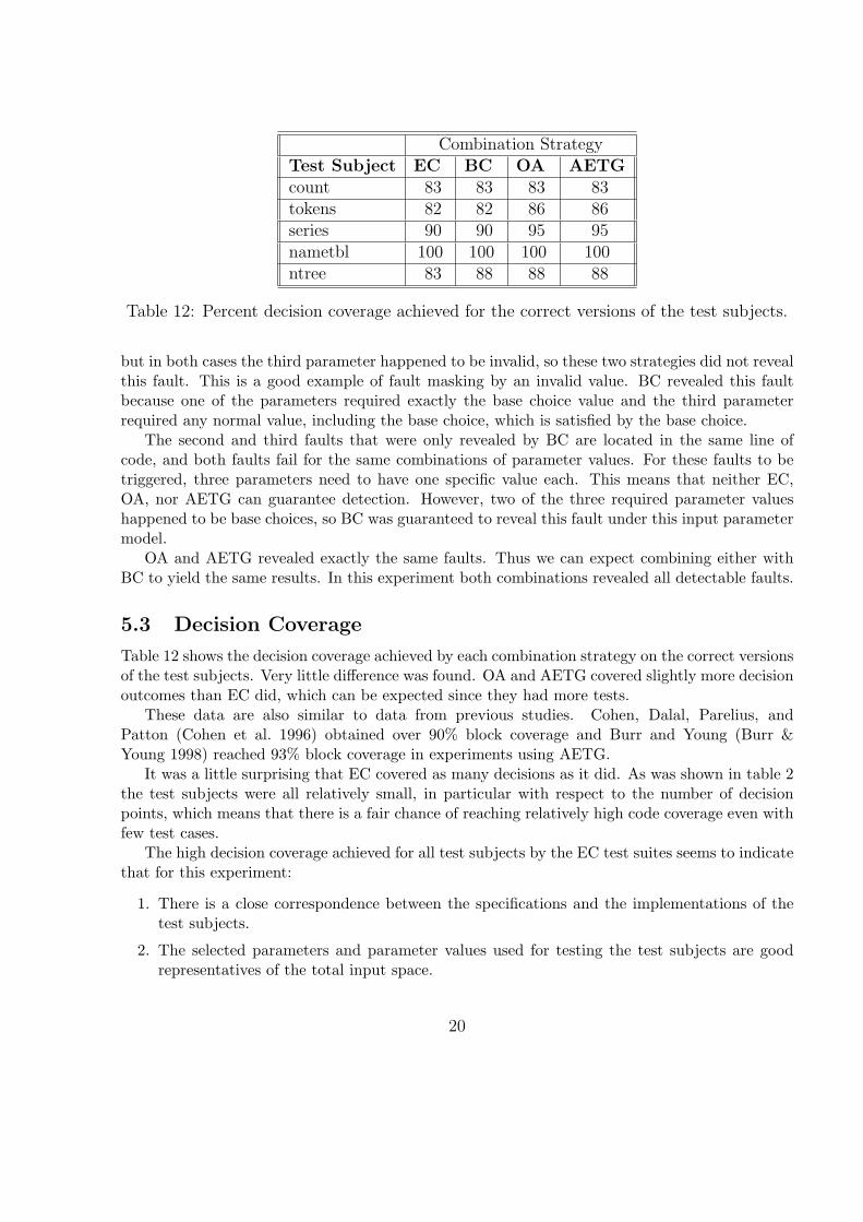
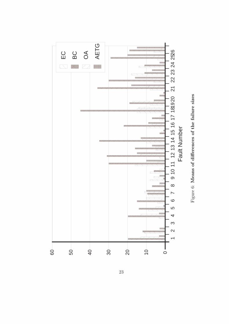
An initial observation of this data shows that BC is unusual. Specifically, BC has either thehighest or the lowest failure size for 24 of the 26 faults. For many faults, for instance fault 1in count, fault 4 in series, and fault 7 in ntree, the failure sizes of BC differ from the othersby a great deal. To evaluate how different the failure sizes for BC are from the failure sizes forthe other criteria, we computed the means of the failure sizes for each fault. Then, for each

21

combination strategy we computed the variance of the distances between the actual failure sizesand the means for each fault. These results are displayed in the bar chart in figure 6. The resultingvariances for each combination strategy were then compared using an F-test. With a hypothesisthat the variance of distances between the actual failure sizes and the means for each fault for BCis different from the corresponding variances of the other three combination strategies, the resultsare that the hypothesis cannot be rejected with a significance level of 98%.

BC behaves differently because of the way it selects values. The other combination strategieschoose values in an approximately uniform distribution, that is, all the values appear about thesame number of times in the test suite. In a BC test suite, however, the base choice values appearmore often because every test case is derived from the base test case.

Faults that are triggered by base choice values will result in BC having a higher failure sizethan the other combination strategies because the base choice values appear so frequently. Theopposite is also true; when faults are triggered by non-base choice values, BC will have lowerfailure size than the other combination strategies.

6 Discussion and Conclusions

Some faults were not found by any combination strategy, yet all the strategies found most ofthe faults. At the same time, 100% decision coverage was only reached in one program. Thuswe conclude that combination strategies should be combined with other methods such as codecoverage-based methods. The following subsections discuss more detailed results.

22

1 10

9

8 7

6 5

4 3

2 11

19

20

18

17

16

15

14

13

12

21

26

25

24

23

22

60

50

40

30

20

10

0 ��� �� ��� �� ���� �� ����� �� ���� ��� �� �� �� �� ��� ���� ��� ��� �� ���� ��� ��� ���� �� �� ��� ��� �� ��� �� �� ������ ��� �� �� ��� ���� ���� �� �� �� �� �� �� ������ ��� �� �� �� ��� �� �� �� �� ��� �� �� ������ �� �� �� �� ����� �� ��E

C

AE

TG

OA

BC

Fau

lt N

umbe

r

Fig

ure

6:M

eans

ofdiff

ere

nce

softh

efa

ilure

size

s

23

6.1 Fault Finding Abilities of Combination Strategies

This subsection tries to make some general observations about the abilities of the combinationstrategies to find faults. These observations are based partly on the data, partly on experienceapplying the strategies, and partly on an analysis of the theory behind the combination strategies.The data showed that EC revealed many faults by coincidence. This leads to the conclusion thatthe result of applying EC is too unpredictable to be really useful for the tester.

In this experiment the combination strategies are used solely in a black-box manner. Thatis, they only use information from the specifications when designing the test cases. It is worthstressing that there can be no guarantees that all faults will be found by this approach. This wasalso the case in this experiment, where three faults were missed because they were implementationrelated, as described in section 5.2.

BC is different from the other strategies because semantic (or domain) knowledge is used tochoose base values. Choosing base values is very simple, but the choice of base values directlyaffects all of the tests. Ammann and Offutt (Ammann & Offutt 1994) recommend choosing themost commonly used value (based on expected user behavior). Analysis and the data indicatethat this means BC tests will be more likely to find faults in parts of the program that are mostoften used. As a result of BC satisfying single error coverage, no test case will contain more thanone invalid parameter value, making it less likely that faults will be masked. This conclusion isbased on analysis of the faults that only BC revealed.

A weakness of BC showed up in test problems where some parameters contain two or morevalues that will be used about the same number of times by the user, that is, there is more thanone base choice candidate. In a BC test suite, each non-base choice value will only occur once,which discriminates the other commonly used values. Thus, BC is probably most effective wheneach parameter contains one obvious base choice value.

Although OA and AETG generate test suites with different contents, they both satisfy pair-wise coverage, and thus have similar performance. Also, the sizes of test suites generated by OAand AETG are similar. Hence, the practicing tester should choose based on other factors, forinstance ease-of-use.

It seems easier to automate the AETG strategy than the OA strategy (this is supported bythe fact that there is a tool for AETG). It is also straightforward to extend AETG to generatet-wise tests, where t is an arbitrary number. Automating OA is quite difficult.

AETG can also start with an existing test suite and extend it to satisfy pair-wise (or t-wise)coverage. For example, BC tests could be created, and then extended with AETG to satisfypair-wise coverage.

The pair-wise coverage property of OA and AETG gives best results for test subjects wherethere are many valid values of each parameter, which is when BC is least effective. For testproblems with many invalid values for each parameter, when BC is most effective, the pair-wisestrategies may mask faults, that is, when tests cover several parameter value pairs with multipleinvalid values, the effects of some parameters may be masked by others. This was also observed byCohen et al. (Cohen et al. 1997). In test subjects where parameters contain both several valid andseveral invalid values it seems to be the case that a combination of BC and a pair-wise strategy isrequired to yield the best effectiveness.

To summarize, our assessment is that BC and AETG should be combined to get the best

24

effects. The BC tests will provide a focus on user behavior and reduce the risk of fault masking,and then extended with pair-wise tests for faults that appear in parts of the program that are notused as much.

6.2 Input Parameter Modeling

A final observation relates to modeling the input parameters. Test engineers often need to choosebetween representing some aspect of the input space as either a separate parameter or by addingmore values to another parameter. The choice should depend on which combination strategy isused.

Given a fixed number of parameters values, for EC, BC, OA, and AETG, it is better to havemany parameters with few values, but for AC it is better to have few parameters with many values.It should be noted that this analysis is purely based on cost; no data exists on the relative faultfinding abilities.

Piwowarski, Ohba, and Caruso (Piwowarski et al. 1993) showed the applicability of refining theinput parameter model by monitoring the code coverage achieved by the generated test suite. Thissuggests that code coverage may be used both to validate the effectiveness of the input parametermodel and to identify parts of the code that should be tested with other means.

6.3 Recommendations

The following recommendations summarize the findings.

• Combination strategies are useful test methods but need to be complemented by code cov-erage.

• When time is a scarce resource, use BC. Its advantages are its low cost and its user orienta-tion.

• When there is enough time, combine BC with AETG. BC reduces the likelihood of maskingof faults, and AETG guarantees pair-wise coverage.

• For the less demanding strategies, when identifying parameters and equivalence classes thetest suite will be smaller if more parameters with few values are used than if few parameterswith many values are used.

7 Related Work

An interesting example of how different testing methods can be compared is described by Reid (Reid1997). Software from a real avionics system was used. All existing trouble reports from the firstsix months of operation were collected. These faults were investigated and any fault that couldhave been found during component testing were identified and used in the study. Each fault wasanalyzed to determine the complete set of input values that would trigger that fault, call thefault-finding set. Independently of the fault analysis, boundary value analysis and equivalencepartitioning were used to partition the input space into test case sets. Under the assumption that

25

each test case has the same probability of being selected, the effectiveness of each testing methodwas calculated as the probability that all faults will be revealed. Reid found that the mean prob-ability for fault detection for boundary value analysis is 0.73 and for equivalence partitioning it is0.33. An important contribution by this research is the method of comparison, which can be usedto compare any type of testing methods.

Several studies have compared the effectiveness of different combination strategies. By farthe most popular property used to compare combination strategies is number of test cases gen-erated for a specific test subject. This is easy to compute and particularly interesting for thenon-deterministic and greedy combination strategies, since the size of the test suite cannot bedetermined algebraically. Several papers have compared a subset of the combination strate-gies that satisfy 2-wise and 3-wise coverage (Lei & Tai 1998, Williams 2000, Shiba, Tsuchiya &Kikuno 2004, Cohen, Gibbons, Mugridge & Colburn 2003). The combination strategies performsimilarly with respect to the number of test cases generated in all of these comparisons.

Since the number of test cases does not clearly favor one particular combination strategy, someauthors have also compared the strategies with respect to time consumption, that is, the executiontime for the combination strategy to generate its test cases. Lei and Tai (Lei & Tai 2001) show thatthe time complexity of their combination strategy called In-Parameter-Order (IPO) is superior tothe time complexity of AETG. IPO has a time complexity of O(v3N2log(N)) and AETG has atime complexity of O(v4N2log(N)), where N is the number of parameters, each of which has vvalues.

Further, Williams (Williams 2000) reports on a refinement of OA called Covering Arrays (CA)that outperforms IPO by almost three orders of magnitude for the largest test subjects in theirstudy, in terms of time taken to generate the test suites. Finally, Shiba et al. (Shiba et al. 2004)show some execution times but the executions have been made on different target machines so theresults are a bit inconclusive.

8 Future Work

There are still several questions to be answered before concluding that combination strategiescan be used in an industrial setting, and other questions about how best to apply them. A firstquestion is about the best method to use for input parameter modeling. This experiment keptthe model stable and modified the strategy used to generate tests. It would also be useful toprecisely describe different (repeatable) methods for generating the input model and then performanother experiment that varies them. A secondary question, of course, would be whether the twovariables interact, that is, whether changing the input parameter modeling method would affectwhich combination strategies work best.

The experiment in this paper also did not directly handle conflicts among parameter values.The best way to handle conflicts needs to be determined, and how they interact with strategies andinput modeling methods also needs to be investigated. AETG has a conflict handling mechanismalready built into the algorithm (Cohen et al. 1997). Other conflict handling mechanisms areindependent of the combination strategies (Grindal et al. 2005), and a follow-up study of theperformance of these is currently in process.

This experiment was performed in a laboratory setting and used fairly small programs. This

26

limits the external validity of the results. It would be helpful to try some of these techniques inan industrial setting, both to assess their effectiveness and to assess their true cost.

An obvious result from this study is the conclusion that the contents of the input parametermodel affects the test results in a major way. For instance, in section 5.2 it was shown that thenumber of t-factor faults for each t may differ for different contents of the input parameter model.One plan is to determine how sensitive the test results are to the actual contents of the inputparameter model.

In the future, we hope to further develop the tools used in this experiment to be more robust,include more automation, and to be more general. An ultimate goal, of course, is to completelyautomate the creation of tests. It seems likely that the test engineer would always need to developthe input parameter model and the expected results for each selected test case, but it should bepossible to automate the rest of the test process.

We also hope to formalize the description of different types of faults. It would also be interestingto examine variants of combination strategies, for example, using the complete BC test suite asinput to the AETG algorithm.

It might also be useful to empirically compare combination testing strategies with other testmethods, for instance by the method described by Reid (Reid 1997).

Related to the fault-finding sets studied by Reid is the number of combinations that will reveal acertain fault. It was shown in section 5.2 that two factors influence whether combination strategiesreveal a fault. One is the number of parameters involved in triggering the failure (t-factor), andthe other is how many combination of values of those parameters that will trigger that fault. Aswas also observed by Cohen et al. (Cohen et al. 1994), it would be interesting to study faults inreal-world applications to determine the properties with respect to fault detection.

9 Acknowledgments

First and foremost we owe our gratitude to Dr Christopher Lott for generously supplying all thematerial concerning the test subjects and being very helpful in answering our questions. Next, weare indebted to the anonymous referees who offered many helpful suggestions.

Then, we are also indebted to many of our colleagues in the computer science departmentat the University of Skovde. Louise Ericsson gave us helpful hints when we were lost trying todebug the Prolog program for generating orthogonal arrays. Marcus Brohede and Robert Nilssonsupplied valuable tips during the set up of the compiler environment. Sanny Gustavsson, JonasMellin, and Gunnar Mathiason gave us general support and good ideas.

Finally, Thomas Lindvall and Asa Grindal gave helpful advice during the analysis of the resultsand the writing process respectively.

References

Ammann, P. E. & Offutt, A. J. (1994). Using formal methods to derive test frames in category-partition testing, Proceedings of the Ninth Annual Conference on Computer Assurance (COM-PASS’94),Gaithersburg MD, IEEE Computer Society Press, pp. 69–80.

27

Anderson, T., Avizienis, A., Carter, W., Costes, A., Christian, F., Koga, Y., Kopetz, H., Lala,J., Laprie, J., Meyer, J., Randell, B. & Robinson, A. (1994). Dependability: Basic Conceptsand Terminology, Technical report, IFIP. WG 10.4.

Archibald, R. (1992). Managing High-Technology Programs and Projects, John Wiley and sons,Inc.

Bache, R. (1997). The effect of fault size on testing, The Journal of Software Testing, Verification,and Reliability 7: 139–152.

Basili, V. R. & Rombach, H. D. (1988). The TAME project: Towards improvement-orientedsoftware environments, IEEE Transactions on Software Engineering SE-14(6): 758–773.

Basili, V. & Selby, R. (1987). Comparing the Effectiveness of Software Testing Strategies, IEEETransactions on Software Engineering SE-13(12): 1278–1296.

Basili, V., Shull, F. & Lanubile, F. (1999). Using experiments to build a body of knowledge,Perspectives of System Informatics, Third International Andrei Ershov Memorial Conference(PSI 99), Akademgorodok, Novosibirsk, Russia, July 6-9, 1999, Proceedings, pp. 265–282.

Briand, L. & Pfahl, D. (1999). Using simulation for assessing the real impact of test coverageon defect coverage, Proceedings of the International Conference on Software Maintenance(ICSM99), 30th of Aug - 3rd Sept, 1999, Oxford, The UK, pp. 475–482.

Brownlie, R., Prowse, J. & Phadke, M. (1992). Robust Testing of AT&T PMX/StarMAIL usingOATS, AT&T Technical Journal 71(3): 41–47.

Burr, K. & Young, W. (1998). Combinatorial test techniques: Table-based automation, test gen-eration and code coverage, Proceedings of the International Conference on Software Testing,Analysis, and Review (STAR’98), San Diego, CA, USA, pp. 26–28.

Cohen, D., Dalal, S., Fredman, M. & Patton, G. (1997). The AETG System: An Approach to Test-ing Based on Combinatorial Design, IEEE Transactions on Software Engineering 23(7): 437–444.

Cohen, D., Dalal, S., Kajla, A. & Patton, G. (1994). The automatic efficient test generator (AETG)system, Proceedings of Fifth International Symposium on Software Reliability Engineering(ISSRE’94), Los Alamitos, California, USA, November 6-9, 1994, IEEE Computer Society,pp. 303–309.

Cohen, D., Dalal, S., Parelius, J. & Patton, G. (1996). The Combinatorial Design Approach toAutomatic Test Generation, IEEE Software 13(5): 83–89.

Cohen, M., Gibbons, P., Mugridge, W. & Colburn, C. (2003). Constructing test cases for in-teraction testing, Proceedings of the 25th International Conference on Software Engineering,(ICSE’03), Portland, Oregon, USA, May 3-10, 2003, IEEE Computer Society, pp. 38–48.

Dalal, S. & Mallows, C. (1998). Factor-Covering Designs for Testing Software, Technometrics50(3): 234–243.

Dunietz, I., Ehrlich, W., Szablak, B., Mallows, C. & Iannino, A. (1997). Applying design ofexperiments to software testing, Proceedings of 19th International Conference on SoftwareEngineering (ICSE’97), Boston, MA, USA 1997, ACM, pp. 205–215.

28

Frankl, P., Hamlet, R., Littlewood, B. & Stringini, L. (1998). Evaluating Testing Methods byDelivered Reliability, IEEE Transactions on Software Engineering 24: 586–601.

Grindal, M., Lindstrom, B., Offutt, A. J. & Andler, S. F. (2003). An Evaluation of CombinationStrategies for Test Case Selection, Technical Report, Technical Report HS-IDA-TR-03-001,Department of Computer Science, University of Skovde.

Grindal, M., Offutt, A. J. & Andler, S. F. (2005). Combination testing strategies: A survey,Software Testing, Verification, and Reliability 15(3): 167–199.

Harman, M., Hierons, R., Holocombe, M., Jones, B., Reid, S., Roper, M. & Woodward, M. (1999).Towards a maturity model for empirical studies of software testing, Proceedings of the 5thWorkshop on Empirical Studies of Software Maintenance (WESS’99), Keble College, Oxford,UK.

Kamsties, E. & Lott, C. (1995a). An Empirical Evaluation of Three Defect Detection Techniques,Technical Report ISERN 95-02, Dept of Computer Science, University of Kaiserslauten.

Kamsties, E. & Lott, C. (1995b). An empirical evaluation of three defect detection techniques, Pro-ceedings of the 5th European Software Engineering Conference (ESEC95), Sitges, Barcelona,Spain, September 25-28, 1995.

Kropp, N., Koopman, P. & Siewiorek, D. (1998). Automated robustness testing of off-the-shelfsoftware components, Proceedings of FTCS’98: Fault Tolerant Computing Symposium, June23-25, 1998 in Munich, Germany, IEEE, pp. 230–239.

Lei, Y. & Tai, K. (1998). In-parameter-order: A test generation strategy for pair-wise test-ing, Proceedings of the third IEEE High Assurance Systems Engineering Symposium, IEEE,pp. 254–261.

Lei, Y. & Tai, K. (2001). A Test Generation Strategy for Pairwise Testing, Technical ReportTR-2001-03, Department of Computer Science, North Carolina State University, Raleigh.

Lindstrom, B., Grindal, M. & Offutt, A. J. (2004). Using an existing suite of test objects: Experi-ence from a testing experiment, Workshop on Empirical Research in Software Testing, ACMSIGFOST Software Engineering Notes, Boston, MA, USA.

Lott, C. (n.d.). A repeatable software experiment, URL:www.chris-lott.org/work/exp/ .

Lott, C. & Rombach, H. (1996). Repeatable Software Engineering Experiments for ComparingDefect-Detection Techniques, Journal of Empirical Software Engineering 1(3): 241–277.

Mandl, R. (1985). Orthogonal Latin Squares: An application of experiment design to compilertesting, Communications of the ACM 28(10): 1054–1058.

Miller, J., Roper, M., Wood, M. & Brooks, A. (1995). Towards a benchmark for the evaluation ofsoftware testing techniques, Information and Software Technology 37(1): 5–13.

Musa, J. (1993). Operational profiles in software-reliability engineering, IEEE Software 10: 14–32.

Myers, G. (1979). The Art of Software Testing, John Wiley and Sons.

Ntafos, S. C. (1984). On Required Element Testing, IEEE Transactions on Software EngineeringSE-10: 795–803.

29

Offutt, A. J. & Hayes, J. H. (1996). A semantic model of program faults, Proceedings of the 1996International Symposium on Software Testing, and Analysis, ACM Press, San Diego, CA,pp. 195–200.

Offutt, A. J., Xiong, Y. & Liu, S. (1999). Criteria for generating specification-based tests, FifthIEEE International Conference on Engineering of Complex Systems (ICECCS’99),Las VegasNV, IEEE, pp. 119–129.

Ostrand, T. & Balcer, M. (1988). The Category-Partition Method for Specifying and GeneratingFunctional Tests, Communications of the ACM 31(6): 676–686.

Piwowarski, P., Ohba, M. & Caruso, J. (1993). Coverge measure experience during functiontest, Proceedings of 14th International Conference on Software Engineering (ICSE’93), LosAlamitos, CA, USA 1993, ACM, pp. 287–301.

Reid, S. (1997). An empirical analysis of equivalence partitioning, boundary value analysis andrandom testing, Proceedings of the 4th International Software Metrics Symposium (MET-RICS’97), Albaquerque, New Mexico, USA, Nov 5-7, 1997, IEEE, pp. 64–73.

Shiba, T., Tsuchiya, T. & Kikuno, T. (2004). Using artificial life techniques to generate test casesfor combinatorial testing, Proceedings of 28th Annual International Computer Software andApplications Conference (COMPSAC’04) 2004, Hong Kong, China, 28-30 September 2004,IEEE Computer Society, pp. 72–77.

So, S., Cha, S., Shimeall, T. & Kwon, Y. (2002). An empirical evaluation of six methods to detectfaults in software, Software Testing, Verification and Reliability 12(3): 155–171.

Wallace, D. R. & Kuhn, D. (2001). Failure Modes In Medical Device Software: An Analysis Of 15Years Of Recall Data, International Journal of Reliability, Quality, and Safety Engineering8(4): 351–371.

Williams, A. (2000). Determination of test configurations for pair-wise interaction coverage, Pro-ceedings of the 13th International Conference on the Testing of Communicating Systems(TestCom 2000), Ottawa, Canada, August 2000, pp. 59–74.

Williams, A. & Probert, R. (1996). A practical strategy for testing pair-wise coverage of networkinterfaces, Proceedings of the 7th International Symposium on Software Reliability Engineer-ing (ISSRE96), White Plains, New York, USA, Oct 30 - Nov 2, 1996, pp. 246–254.

Wood, M., Roper, M., Brooks, A. & Miller, J. (1997). Comparing and combining software defectdetection techniques: A replicated study, Proceedings of the Sixth European Software Engi-neerng Conference (ESEC/FSE 97), Springer Verlag, Lecture Notes in Computer Science Nr.1013, pp. 262–277.

Woodward, M. R. & Al-Khanjari, Z. A. (2000). Testability, fault size and the domain-to-rangeratio: An eternal triangle, Proceedings of the 2000 ACM SIGSOFT international symposiumon Software testing and analysis (ISSTA ’00), ACM Press, Portland, Oregon, USA, pp. 168–172.

Yin, H., Lebne-Dengel, Z. & Malaiya, Y. (1997). Automatic Test Generation using CheckpointEncoding and Antirandom Testing, Technical Report CS-97-116, Colorado State University.

30

Zweben, S. & Heym, W. (1992). Systematic Testing of Data Abstractions Based on SoftwareSpecifications, Journal of Software Testing, Verification, and Reliability 1(4): 39–55.

31