An European Labour Market model using GIS

extension and analysis on network resilience and

robustness

Pietro Saggese

25/06/2015

Introduction

The purpose of this work, consisting of two separated and independent parts,is mainly to study the european labour market, following an agent-basedmodel approach. Two typologies of agents are created: householders, dividedin employed and unemployed, and �rms, which interact with householdershiring and paying them, while the unemployed ones move looking for a work.Firms choose �rst the nearest householders, then they establish a range inwhich search for other workers, and select the ones with the highest workskills. The graphic interface has been implemented so as to represent thegeographic map of Europe, in order to render the presentation of dynamicsand results more comprehensible, clear and intuitive - but also for aestheticalreasons; to avoid an overload of the program and excessive slowness, wepresent only six countries, since we consider them representative of the actual- economical and political - situation of Europe. The selected countries are:United Kingdom, Germany, France, Italy, Spain and Greece.

In the second part of the simulation, instead, the target is to study theensemble of �rms as a network; for simplicity, there is no distinction betweenintermediate or �nal goods. However, we can think at this network as anensemble of �rms producing some goods not better speci�ed but reciprocallynecessary to produce their own �nal good. The underlying idea is the intu-ition that �rms are strictly tied in each economy and the wellness of a partof the economy a�ects directly many other sectors: an interesting way toface up to this themathic is to implement a network-based approach. Here,for example, we simulate the degree of interconnection in the economy bysetting a variable parameter a�ecting the biggest distance possible to createa link between two �rms. What would happen to the network if we remove a�rm from it and some rings of this entire production chain were broken? Towhat extent the network would remain fully connected or operative? Thiswork can be a support when we ask ourselfs these questions and can be animportant benchmark for further and more complicated analyses, as the caseof a network with an intermediate good and one or more �nal goods, or thecase of a production chain composed by more intermediate goods necessaryto obtain the �nal good. Hence, in this paper we study the resilience androbustness of the network, by comparing two di�erent situations: �rst, weeliminate at each loop a �rm from the network, randomly; second, we cal-culate the betweennes of each �rm and we remove the one with the highestvalue; the result we are interested in is the comparison of the giant com-ponent's dimension variation and the degree distribution after 5, 10 and 15attacks to the network.

To implement these features Netlogo has been used, which is an agentbased-model programming language that allows to generate agents and letsthem interact in a graphic interface. There are three principal kinds ofagents: turtles, patches and links. Each one of them can be created with

1

characterizing features and variables; in particular, Netlogo supplies the pos-sibility to divide furthermore each typology of agents in subclasses, calledbreeds. In our case, e.g. , turtles are subdivided in two breeds, that is, �rmsand householders. Another foundamental feature of Netlogo is the possibil-ity to interact with the interface, since it gives the possibility to an externalobserver, which runs the code, of interacting with it, changing the value ofsome parameters in a range, switching on/o� given variables, asking to theinterface to report the value of variables of agents we are interested in.

The Code and The Model

Part 1: Labour Market and GIS

Figure 1: Netlogo's interface

Since the main goal of this �rst part is to model the European labour mar-ket, the �rst idea has been to try to improve the graphic interface of Netlogo,associating a map of the Europe to the patches. Luckily, one of the mostinteresting peculiarities of Netlogo is the possibility of adding extensions,which allow to integrate his features and to do more complex operations.Specially, one of these extensions �ts perfectly our aims: the GIS extension.In fact, the acronym GIS means Geographic Information System, and in theinformatic language it speci�es a system designed to capture, store, manip-ulate, analyze, manage and present all types of spatial or geographical data.A GIS software allows to combine geographical maps, to execute statisticalanalysis on data and manage them through a database. In our simulation,

2

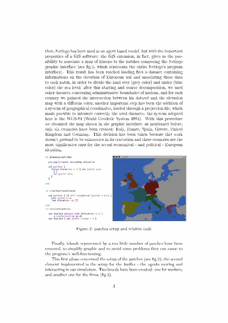
then, Netlogo has been used as an agent based model, but with the importantproperties of a GIS software: the GIS extension, in fact, gives us the pos-sibility to associate a map of Europe to the patches composing the Netlogographic interface (see �g.1, which represents the entire Netlogo's programinterface). This result has been reached loading �rst a dataset containinginformations on the elevation of European soil and associating these datato each patch, in order to divide the land over (grey color) and under (bluecolor) the sea level; after this starting and coarse decomposition, we usedother datasets concerning administrative boundaries of nations, and for eachcountry we painted the intersection between his dataset and the elevationmap with a di�erent color; another important step has been the addition ofa system of geographical coordinates, loaded through a projection �le, whichmade possible to intersect correctly the used datasets: the system adoptedhere is the WGS-84 (World Geodetic System 1984). With this procedurewe obtained the map shown in the graphic interface; as mentioned before,only six countries have been created: Italy, France, Spain, Greece, UnitedKingdom and Germany. This decision has been taken because this workdoesn't pretend to be exhaustive in its tractation and these countries are themost signi�cative ones for the actual economical - and political - Europeansituation.

Figure 2: patches setup and relative code

Finally, islands represented by a too little number of patches have beenremoved, to simplify graphic and to avoid some problems they can cause tothe program's well-functioning.

This �rst phase concerned the setup of the patches (see �g.2); the secondelement implemented is the setup for the turtles - the agents moving andinteracting in our simulation. Two breeds have been created: one for workers,and another one for the �rms (�g.3).

3

Figure 3: householders and �rms setup

Householders are created with some variables, a�ecting their behaviorwhen simulation is run: the incomes they receive when they work, theirworking skills and their propension to consumption; similarly, �rms have aweight on market, which determines in what order �rms will hire people.All agents are generated randomly on the graphic interface, but a commandmakes them move to countries and recolours them with the color of thecountry where they move to. Finally, with a probability of 10%, peopleis transferred to another country, to simulate the presence of non residenthouseholders in each nation. It is then always possible to check how manyresidents and non residents live in a country.

Another important Netlogo's feature is the possibility, for the observer, tointeract from the interface with the code: for example, here the use of slidershas been introduced to control and variate the number of householders and�rms created at each simulation(see �g.1). The number of workers hired byeach �rm, instead, is �xed to 8 (the choice of this number is arbitrary): thisimplies, as speci�ed in a note in the interface, that we have to generate atleast 8 workers times the number of �rms; otherwise, an error message willbe shown in the output.

Once the setup procedure is done, agents start to interact: the �rst stepconsists in a hiring phase, during which �rms - in order of importance on

4

Figure 4: Labour Market network before production delocalisation and pro-cedure to hire workers

the market - hire the nearest disposable workers, neglecting their ability towork; in the interface, a link between �rm and employed workers appears, toillustrate the relation between these agents. A radius, equal to the distancefrom the farthest employed, is established (and shown in the label): in future,each �rm will look for other workforce only in this range and not further.This step can however create some problems, because sometimes �rms hireworkers too far from them; in other cases, all workers of a �rm are in acountry and their �rm is established in another one (see �g.4).

Figure 5: Labour Market network after production delocalisation and code

It is quite unreal, and also anti-aesthetic: for this reason, it has beendecided to overcome the problem by simulating the delocalisation of the

5

production (see �g.5): through an if cycle, when a �rm hires too far workersor at least 4 non residents, the program looks for areas with an high densityof unemployed householders and moves there the selected �rm. To easillykeep trace of the original country, links with workers of delocalised �rmswill be painted with the original country's color. Fig.5 shows the di�erencebefore and after the delocalisation procedure. The used code is really similarto the one represented in �g.4.

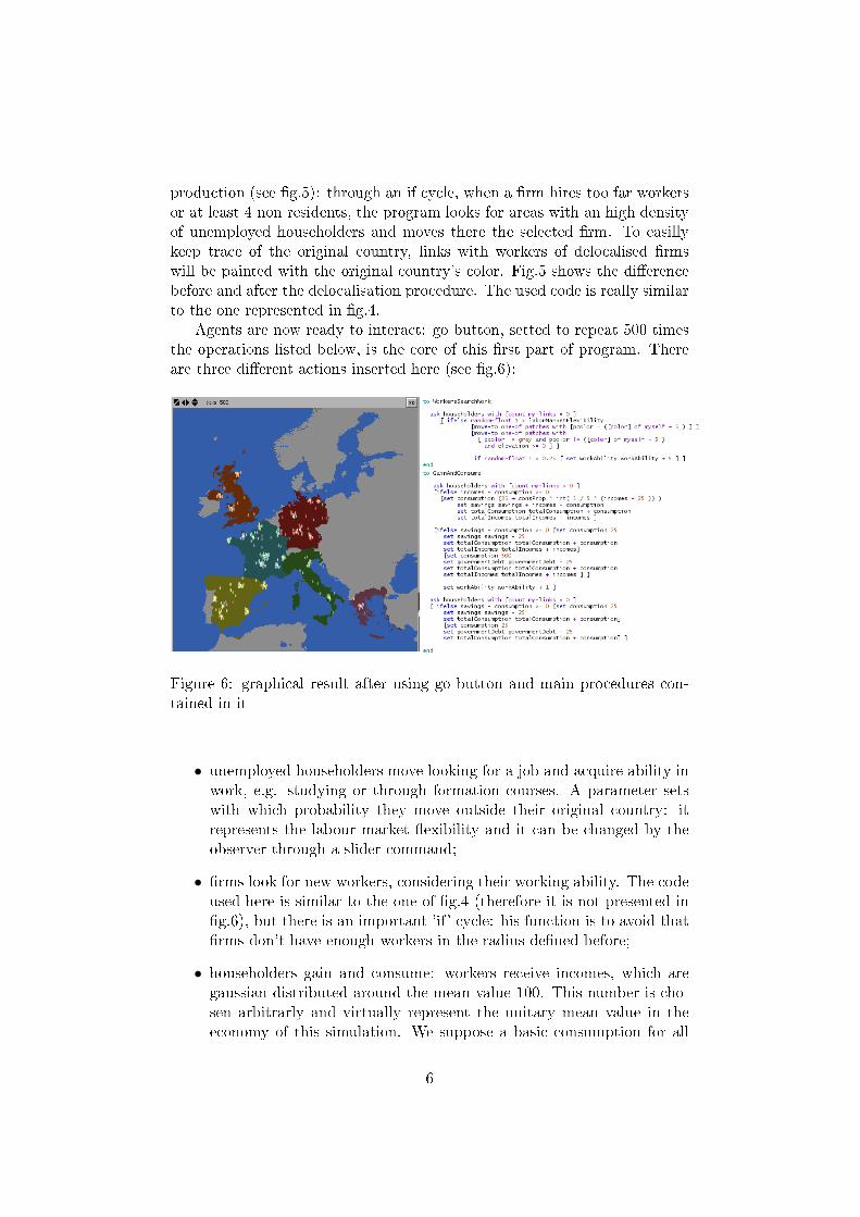
Agents are now ready to interact: go button, setted to repeat 500 timesthe operations listed below, is the core of this �rst part of program. Thereare three di�erent actions inserted here (see �g.6):

Figure 6: graphical result after using go button and main procedures con-tained in it

• unemployed householders move looking for a job and acquire ability inwork, e.g. studying or through formation courses. A parameter setswith which probability they move outside their original country: itrepresents the labour market �exibility and it can be changed by theobserver through a slider command;

• �rms look for new workers, considering their working ability. The codeused here is similar to the one of �g.4 (therefore it is not presented in�g.6), but there is an important 'if' cycle: his function is to avoid that�rms don't have enough workers in the radius de�ned before;

• householders gain and consume: workers receive incomes, which aregaussian distributed around the mean value 100. This number is cho-sen arbitrarly and virtually represent the unitary mean value in theeconomy of this simulation. We suppose a basic consumption for all

6

the householders, even if unemployed: if they have enough savings theywill use them; otherwise, they will receive subsidies from the govern-ment (which accumulates a debt). Employed ones, instead, have anhigher level of consumption, function of their propension to spend andof the incomes perceived.

This last point represent a very simpli�ed example of national account-ing and it is presented in the interface through six monitors showing totalconsumption (of each householder, in all the 500 steps), total savings, totalincomes and government debt (that is, government spending). We assess hisvalidity summing consumption and savings, comparing them with the sumof government debt and incomes.

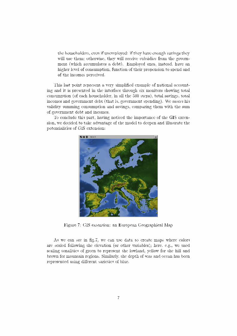
To conclude this part, having noticed the importance of the GIS exten-sion, we decided to take advantage of the model to deepen and illustrate thepotentialities of GIS extension:

Figure 7: GIS extension: an European Geographical Map

As we can see in �g.7, we can use data to create maps where colorsare scaled following the elevation (or other variables); here, e.g., we usedscaling tonalities of green to represent the lowland, yellow for the hill andbrown for mountain regions. Similarly, the depth of seas and ocean has beenrepresented using di�erent varieties of blue.

7

Part 2: Network analysis

The second part has a di�erent approach and the goal is to show some prop-erties of a network, whose nodes are constituted by the �rms. As mentionedabove, this network aims to represent the interconnection existing betweenthe di�erent sectors of a real country economy. Hence, as shown in �g.8,links between �rms have been created: for simplicity, the parameter set-ting whether the connection exists or not is the physical distance betweenthe nodes; this parameter can be modi�ed by the observer through a slidercommand put in the interface. We hide then the householders, to make theinterface more comprehensible, and we link the �rms; an output monitor iscreated, to show the agentset containing all the linked �rms.

Figure 8: procedure to link �rms and calculate Betweenness; graphical result

The crucial part of this second code section consists in a procedure whichcalculates the betweenness of each �rm at each step: this is foundamentalfor our purposes, since it allows us to compare what happens if a node fromthe network is removed randomly or if the node with highest betweenness isdeleted (and for this reason, now �rms labels show how this value varies ateach step). In network theory, in fact, those two di�erent attacks are calledrandom failure - random processes a�ecting all the nodes with the sameprobability - and focused attacks - �nalized to destroy intentionally the net-work: in this case, the "focus" is on the betweenness variable. Studyinghow the networks respond to this di�erent attacks it is possible to determinesome important properties of a network, like resilience, that is the abilityof a network to provide and maintain an acceptable level of service whenfacing faults and challenges to normal operation; specially, we are interestedhere in analysing the robustness of a network, which is a measure of its re-

8

silience (in terms of connectivity) to the removal of edges or vertices: we canimagine it, then, as the ability of a netowrk to resist to node removals. Thisprocedure is shown in �g.8 (procedure 'to showBetweenness'): betweennes is�rst calculated for each �rm, then �rms sizes and colors are normalized andscaled to depict intuitively the value of the betweenness; darker colors andbigger shapes correspond to higher values.

To simulate the two attacks to the network, we use two di�erent com-mands, shown in �g.9: the �rst one removes nodes sorted by betweenness,the second removes a �rm randomly; both evaluate again the betweenness atthe end of the procedure and give an alarm in the output monitor if no agentsare disposables. It is really important to underline here a crucial feature ofthe program: since we want to compare the e�ect of two di�erent attacks onthe same network, we need to use the command setSeed before setup (seeinterface in �g.1), which allows us to create the same world at each setup,with the same charachteristics and features, variable values, and so on. It ispossible to use both approaches on the same network and comparing themthrough graphs:

Figure 9: random failure and focused attack procedures

Simultaneously, we study other important properties of a network: thedimension of the Giant Component, de�ned as the biggest connected fractionof nodes, absorbing a considerably large part of the entire network if com-pared to the other ones, and the degree distribution of the nodes composingthe network after 5, 10 and 15 attacks to the nodes (the commands to drawthe plots are inserted in procedures of �g.9; the code implementing thosegraphs, instead, is shown in �g.11). To �nd the giant component we use thecode presented in �g.10: this procedure inspects all nodes, asking them if

9

they are already part of a component; at each step the procedure updatesthe dimension of the component being inspected and recognizes which one isthe biggest. Finally, �g.11 shows the code used to depict the graphics: thegoal was to have a visual comparison between results after both a randomand a focused attack on the same network. We show then the degree distri-bution �rst before attacking the network, therefore in the two cases after 5,10, 15 attacks; the other graphic result depicts the di�erent number of steps(attacks) necessary to reduce the dimension of the giant component beneathan arbitrary threshold.

Figure 10: Giant component size detection

Figure 11: plot commands: Giant Component size and degree distributionsafter 5, 10, 15 turns

10

Results

Part 1

For the �rst section, we will compare the results of three di�erent situations:

1. 300 householders and 30 �rms;

2. 550 householders, 60 �rms and halved labour market �exibility;

3. 500 householders and 30 �rms.

As described above, people interact with �rms working and receivingincomes, while unemployed ones look for an employ and try to improve theirworking skills. This procedure is repeated 500 times. The �nal result shownin the graphic interface depicts a mechanism of convergence: since �rms tendto choose the nearest and more skilled workers, when a new worker movesrandomly in the recruiting area of a �rm, if he is better than other workers,he will be assumed. This leads workers, initially randomly distributed oneuropean territory, to be at each step nearer to �rms. After 500 steps, thereare still some unemployed workers moving randomly for a work, but thebiggest fraction of householders will be situated in proximity of the �rmthey work for; this behaviour can be thought, then, as a model representingcities-formation (see �g.12).

Figure 12: cities-formation mechanism and government Debt. 300 house-holders and 30 �rms

Another important element we inspect is the government Debt: in theeconomy of this world, people consume even if they don't have neither worknor savings: in this case, it is assumed that government will help citizens

11

supplying subsidies. Also in this case we can assess a convergence mechanism;government debt is initially set equal to zero and in �g.12 we can see itsresults after 5, 10, 25, 50 and 500 steps: data show how, after few steps inwhich government debt grows quickly, the value tends to a constant; we canthen a�ord a sustainability of this economy with these conditions.

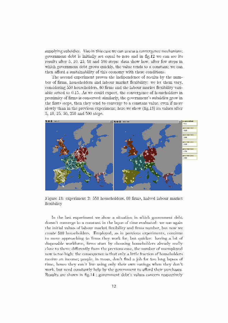
The second experiment proves the indipendence of results by the num-ber of �rms, householders and labour market �exibility: we let them vary,considering 550 householders, 60 �rms and the labour market �exibility vari-able setted to 0.15. As we could expect, the convergence of householders inproximity of �rms is conserved; similarly, the government's subsidies grow inthe �rsts steps, then they tend to converge to a constant value, even if moreslowly than in the previous experiment; here we show (�g.13) its values after5, 10, 25, 50, 250 and 500 steps.

Figure 13: experiment 2: 550 householders, 60 �rms, halved labour market�exibility

In the last experiment we show a situation in which government debtdoesn't converge to a constant in the lapse of time evaluated: we use againthe initial values of labour market �exibility and �rms number, but now wecreate 500 householders. Employed, as in previous experiments, continueto move approaching to �rms they work for, but quicker: having a lot ofdisposable workforce, �rms start by choosing householders already reallyclose to them; di�erently from the previous case, the number of unemployednow is too high: the consequence is that only a little fraction of householdersreceive an income; people, in mean, don't �nd a job for too long lapses oftime, hence they can't live using only their own savings when they don'twork, but need constantly help by the government to a�ord their purchases.Results are shown in �g.14 ; government debt's values concern respectively

12

the steps number 100, 200, 300, 400 and 500.

Figure 14: experiment 3: 500 householders, 30 �rms

13

Part 2

Figure 15: 11 focused attacks: a graphic view of the network

This section is introduced illustrating qualitatively, through a graphicview, the di�erence between the two attacks to the network: �g.15 depictsthe twelve phases of an attack composed by the removal of eleven nodes usinga focused attack, while �g.16 throguh a random attack. We can see somedi�erences: in the �rst case, the focused attack divides quickly the networkin smaller components: after 4 nodes removals, all the United Kingdom's�rms are disconnected by the biggest component; at the �fth attack, thesame happens to the spanish ones. At the sixth step, Greece is completelydisconnected, and after eight turns only France and Italy are still part of thesame network.

Completely di�erent is the behavior in the random case: after 12 stepsalmost all the countries are linked (excepted Greece, which is casually dis-connected at the fourth step), the initial structure is still visible and nodeswith high connectivity have not been removed. We can assume then intu-itively that random case a�ects de�nitely less the network than the focused

14

one, which destroys the network in really few iterations.

Figure 16: 11 random attacks: a graphic view of the network

The main analysis we are interested in, however, is to generate 6 di�er-ent networks and to compare for each one the di�erent e�ects of randomand focused attacks, on giant component size dimension and on the degreedistributions after 5, 10, 15 steps. Fig.17-18 show the results.

We can obtain two main conclusions from this analysis:

• as expected, the giant component size decreases drastically faster whenan attack based on betweenness occurrs, if compared with random ones:we can see in each graph of �g.17 how the green line, representing thebetweenness-based attack, reaches the selected threshold a relativelyhigh number of steps before the violet one (random case). The net-works are then generally resistent and robust to random failures, whileextremely sensible to focused attacks;

• degree distribution tends to reach lower values in the case of betweennesfocused attacks: as we can see in �g.18, all the networks present a

15

lower connectivity (green distribution) when node removal occurs bybetweenness approach. This can be explained by the fact that focusedattacks hit the more connected nodes, while random attacks are casualand then don't recognize the importance of a node in the network.This necessarily leads to a di�erent degree distribution.

Figure 17: giant component size comparison for 6 di�erent networks andrelative initial degree distribution

These results are interesting and important, since some arti�cial net-works, constructed connecting nodes randomly following a probability basedrule - like Erd®s-Rényi's one -, show similar behaviour if attacked randomlyor sorting removed nodes by betweenness; instead, real networks - and thoseconstructed following the Barabási-Albert algorithm, e. g. - have drasticallydi�erent behaviours depending on the attack typology: as in our experiment,

16

a random attack doesn't alter strongly the structure of these networks andtheir robustness is rather high; conversely, real networks aren't robust toattacks focused on degree or on betweenness.

Figure 18: degree distribution comparison for 6 di�erent networks

This could lead to an interesting deepening of this basic model, to inves-tigate on this network and its properties.

17