An Estimator for Some Binary-Outcome Selection Models W ... · An Estimator for Some Binary-Outcome...

P1: GIB

OJ006-01 March 29, 2003 11:46

Political Analysis (2003) 11:111–138DOI: 10.1093/pan/mpg001

An Estimator for SomeBinary-Outcome Selection Models

Without Exclusion Restrictions

Anne E. SartoriDepartment of Politics, Princeton University,

Corwin Hall, Princeton, NJ 08544-1012e-mail: [email protected]

This article provides a new maximum-likelihood estimator for selection models with di-chotomous dependent variables when identical factors affect the selection equation andthe equation of interest. Such situations arise naturally in game-theoretic models whereselection is typically nonrandom and identical explanatory variables influence all decisionsunder investigation. When identical explanatory variables influence selection and a sub-sequent outcome of interest, the commonly used Heckman-type estimators identify fromdistributional assumptions about the residuals alone. When its own identifying assump-tion is reasonable, the new estimator allows the researcher to avoid the painful choicebetween identifying from distributional assumptions alone and adding a theoretically un-justified variable to the selection equation in a mistaken attempt to “boost” identification.The article uses Monte Carlo methods to compare the small-sample properties of theestimator with those of the Heckman-type estimator and ordinary probit.

1 Introduction

Many of the most interesting political phenomena are ones for which the sample is non-randomly selected. Actors’ choices or circumstances determine whether or not they areobserved going to war, casting a vote, or choosing a new form of government after a civilwar. Standard regression techniques such as ordinary least squares and logit/probit yieldinaccurate estimates if some included variable and some omitted variable affect both se-lection into the sample and the subsequent political outcome of interest. The problem ismore serious than many researchers realize: the results obtained with standard techniquesare not even accurate estimates of the effects of the independent variables, conditional ona case being in the sample. A growing number of works in political science therefore usestatistical procedures designed to avoid selection bias (Brehm 1993; Mitchell et al. 1997;Berinsky 1999; Reed 2000; Boehmke 2003).

Author’s note: I am grateful to Chris Achen, Larry Bartels, John Brehm, Gary King, Jeff Lewis, Elie Tamer, JasSekhon, anonymous reviewers, and the audience at the Society for Political Methodology 2001 Summer Meetingfor helpful comments, and to Bo Honore for important references. I also thank Shigeo Hirano for his excellentassistance in making user-friendly the computer program that implements the estimator that this article discusses.Finally, I thank CBRSS at Harvard University for support during the year in which I finished this article. Anyerrors are, of course, my own.

Copyright 2003 by the Society for Political Methodology

111

P1: GIB

OJ006-01 March 29, 2003 11:46

112 Anne E. Sartori

The commonly used Heckman-type selection models (Heckman 1974, 1976, 1979;Achen 1986; Van de Ven and Van Praag 1981; Dubin and Rivers 1990) are appropriate onlywhen at least one “extra” explanatory factor influences selection but not the subsequent out-come of interest (Achen 1986, p. 99).1 Unfortunately, this “extra” exogenous variable oftendoes not exist. The Heckman selection models are estimable without the extra variable,but the results are then based only upon the assumptions about distributional assumptionsabout the residuals rather than upon variation in the explanatory variables.2 No one whohas proposed such an estimator recommends using it with identical explanatory variablesin the two equations. Thus, when theory dictates identical explanatory variables in the twoequations, researchers are left with an unhappy choice: to dredge up an extra explanatoryvariable for the selection equation (leading to specification error if the variable does notbelong there) or to identify only from distributional assumptions about the residuals.

This article proposes a maximum-likelihood estimator for use with identical explanatoryvariables and dichotomous dependent variables that is based upon an additional identifyingassumption: The error term for an observation is the same in the two equations. When theassumption is reasonable, the estimator frees researchers from the choice between Scyllaand Charybdis that I discussed in the previous paragraph. The method that I propose hereis easy to execute.

My identifying assumption rarely will be perfectly true, but it is likely to be reasonableexactly when the researcher believes that identical explanatory factors influence selectionand the subsequent outcome of interest. More specifically, the assumption is likely to be aclose match to reality when three conditions hold: (1) selection and the subsequent outcomeof interest involve similar decisions or goals; (2) the decisions have the same causes; and (3)the decisions occur within a short time frame and/or are close to each other geographically.

As an example, the statistical model that I propose would be a likely candidate formodeling states’ decisions about whether or not to escalate wars. The situation meets thethree conditions: the decision to start a war, or select into the sample, is closely related tothe subsequent decision to escalate the conflict or to continue at the current level; the samefactors (e.g. the balance of forces) are posited to influence both decisions; and the decisionsare likely to occur in the same locations, perhaps within a relatively short time frame.

Of course, researchers sometimes have theoretical reasons to believe that the error termsin the two equations are nearly perfectly correlated (or negatively correlated) even whenone or more of the three conditions is not met. In a recent article, Lemke and Reed (2001)make such an argument about enduring rivalry and war among the major powers. Theyargue that states nonrandomly select into rivalries and that identical explanatory variablesaffect states’ decisions both to become rivals and to go to war. In a companion paper, Ireexamine their results using the statistical model that I propose here (Sartori 2002).3

Although the need for this estimator is not new, it is growing with the use of game-theoretic modeling in political science. Game-theoretic and other rational-expectations

1Van de Ven and Van Praag (1981) and Dubin and Rivers (1990) propose selection estimators for use when boththe selection-stage dependent variable and the outcome-stage dependent variable are dichotomous. Becausethese estimators build closely upon Heckman’s work, I refer to these estimators as “Heckman estimators” or“Heckman-type estimators” in this article.

2Moreover, depending upon the substantive problem, it may be impossible to recover the structural parametersof the underlying model. See Maddala (1999, pp. 231–232).

3Lemke and Reed state no theoretical expectations about the direction of the correlation between the error termsin the selection equation and the outcome equation, but they estimate the correlation as highly negative. In thepresent article, I discuss only a version of my estimator that assumes a correlation of +1. My software includesan option for a correlation of −1. However, as I discuss in my companion paper, I believe that theory points toa highly positive correlation in Lemke and Reed’s case.

P1: GIB

OJ006-01 March 29, 2003 11:46

Binary-Outcome Selection Models 113

models often imply that the same factors influence both selection and a later outcomeof interest. Explanatory variables usually enter a game-theoretic model through the payofffunctions, so that, in many models, identical explanatory variables influence every decisionmade by the actors in the model. In addition, many game-theoretic models represent a seriesof binary choices. Thus, the statistical model that I propose here is appropriate for testingimplications of many game-theoretic models, though it also is useful for testing a broaderclass of models that involve nonrandom selection and identical explanatory variables.

My estimator is an alternative to two procedures previously proposed by politicalscientists for testing game-theoretic models (Smith 1998; Signorino 1999, 2002). Mymethod incorporates a different view of the purpose of a formal model than does Signorino’s.Signorino’s procedure assumes that the formal model is correct and that players “make mis-takes according to some known (or assumed) distribution of errors” (Signorino 1999, p. 282).He derives the likelihood function directly from the model and from these assumptions aboutagent error. In contrast, I see any formal model as a representation of an (important) pieceof reality, rather than a complete depiction of the complex world. For example, a crisisbargaining model may focus on the interaction between two players when in actuality manystates are involved. Thus, there is no reason to believe that the appropriate statistical modelcan be derived directly from the formal model. Rather than give up on estimation entirely,I use the formal model only to derive hypotheses, often through comparative statics. I con-sider the problem of the error structure outside of the formal model and build in the simplestpossible error structure that captures basic features of the substantive situation (nonrandomselection and identical explanatory factors). Regardless of the procedure that one uses to testthem, the hypotheses derived from a game-theoretic model incorporate strategic interactionbecause the game-theoretic model itself is strategic.4

The article is organized as follows. The next section introduces the problem of selec-tion bias and provides intuition about why one should not use Heckman-type models whenthe same variables influence selection and the subsequent phenomenon. The third sec-tion presents the new estimator. The fourth uses Monte Carlo simulations to compare thesmall-sample properties of the new estimator to those of probit and of the version of theHeckman estimator that is intended for dichotomous dependent variables. The fifth brieflydiscusses the comparison paper on enduring rivalries, and the sixth concludes. An appendixpresents proofs of consistency and asymptotic normality. STATA software for implementingthis technique is available on the Political Analysis Web site.

2 Selection Bias and the Disadvantages of the Heckman Estimatorwhen the Independent Variables Are Identical

This section of the article briefly reviews the problem of selection bias and attempts toprovide intuition about why the Heckman estimators are poor choices when the researcherbelieves that identical explanatory variables influence selection and the later equation ofinterest.5 Although my proposed estimator is for use with dichotomous dependent variables,this section considers the simpler situation in which the dependent variable of interest

4Signorino’s statistical procedure attempts to estimate the payoffs of the formal model directly. Such a taskrequires very strong identifying assumptions (Lewis and Schultz 2003), and it has not been shown that it ispossible to estimate all of the parameters of interest separately. My point in the text, however, is about thedesirability, rather than the feasibility, of taking the model so literally.

5The selection equation also is often of interest. I call the second equation the equation of interest because thepurpose of selection modeling is to obtain accurate estimates of the effects of the independent variables in thisequation.

P1: GIB

OJ006-01 March 29, 2003 11:46

114 Anne E. Sartori

is continuous because the issues are more intuitive in this simpler situation. Analogousproblems exist when both dependent variables are dichotomous.

2.1 The Problem of Selection Bias

In Heckman’s oft-cited example, the researcher would like to estimate the effect of edu-cation on women’s wages (Heckman 1974).6 The ordinary least squares (OLS) regressiontechnique would be to estimate the effect of the program using the equation

yi = β′xi + εi , (1)

where i represents a woman in the sample, one variable in xi is the woman’s education,yi measures her wages, and εi is a normally distributed error term. The selection problemis that the sample consists only of women who choose to work. These women may differin important unmeasured ways from women who do not work. For example, women whoare smarter may be more likely to enter the labor force than less-smart women because thesmarter women may anticipate that their intelligence will be recognized on the job, resultingin higher wages.

The selection equation is

Ui = γ′wi + ui , (2)

where Ui represents the utility to woman i of entering the labor force, wi is a vector offactors known to influence a woman’s decision to work, and ui , which is jointly normallydistributed with εi , contains any unmeasured characteristics in equation (2). Instead of Ui ,the researcher observes a dichotomous variable Zi with a value of 1 if the woman entersthe labor force (if Ui > 0) and 0 otherwise. For simplicity’s sake, I assume that educationis the only measurable factor that influences the decision of whether or not to work and thateducation has a positive effect on a woman’s desire to work.

Looking at Eqs. (1) and (2), one can see two kinds of selection effects. First, women withhigh levels of education will be more likely to enter the labor force, and so the researcherwill see a sample of educated women. This nonrandom aspect of the sample is what iscommonly misunderstood to be the problem of “selection bias,” but it alone does not biasestimation of (1). Second, and more importantly, some uneducated women will go to work.These women decide that work is worthwhile because they have a high value on someunmeasured variable, part of ui (in this example, intelligence). Thus, those observationsin the sample for the second equation that have small values of the independent variables(more precisely, small values of γ′wi ) also have large error terms. Those observations inthe selected sample that have larger values of the independent variables have a more usualrange of errors. Whether or not education is correlated with the unmeasured intelligence inthe overall population, these two variables are correlated in the selected sample. Assumingthat intelligence does lead to higher wages, one will underestimate the effect of educationon wages because, in the selected sample, women with little education are unusually smart.7

More formally, as long as the error term in the second equation is correlated with thatin the first (e.g., because intelligence is an unmeasured variable in each equation), theerror term for the sample used in the second-stage estimation is not of mean zero and iscorrelated with the explanatory variable. As Heckman and others have shown, the selection

6I simplify and ad lib upon Heckman’s example here.7The clearest discussion of this problem that I have seen is in Achen (1986, pp. 73–81), which I draw uponheavily here.

P1: GIB

OJ006-01 March 29, 2003 11:46


bias problem in a simple linear model is equivalent to an omitted-variable problem. Giventhat observation i is in the sample,

E(yi ) = β′xi + θ

[φ(γ′wi )

�(γ′wi )

], (3)

where φ is a standard normal distribution and � is a cumulative standard normal distribution(Greene 1993, p. 709). When one estimates equation (1) using OLS, the second term is anomitted variable and the estimates of the βs are inconsistent.

Thus, when selection is nonrandom and error terms are correlated, neglecting to modelselection can be a serious mistake. The estimates are inconsistent, even for the group thatone observes in the sample. In this example, estimation on a group of working women leadsto an inaccurate estimate of how education affects the wages of working women.

2.2 The Heckman Model Applied to Equations with IdenticalExplanatory Variables

Heckman (1979) provides an easy method for obtaining a consistent estimate of β whenthe selection mechanism has a dichotomous outcome (the observation either is selectedinto the sample or not) and the subsequent equation of interest has a continuous dependentvariable. The basic idea is to put the omitted variable illustrated in equation (3) back intothe equation. The two-step procedure is as follows:

1. Estimate the probit equation in (2) above. Using the estimated γs, calculate φ(γ′wi )�(γ′wi )

for each observation i in the selected sample.

2. Estimate β and θ by OLS of y on x and φ(γ′wi )�(γ′wi )

.

The standard errors of the estimates also must be adjusted for the selection process (Greene1993, p. 713).

As long as at least one explanatory variable in the selection equation is not in theequation of interest, this technique is a good one. Frequently, the researcher can find sucha variable, called an exclusion restriction.8 However, in many substantively interestingsituations, all factors that influence selection also influence the subsequent outcome ofinterest. For example, a variable posited to affect a state’s decision about whether or not tobegin an international dispute also invariably affects its decisions about whether or not toescalate the dispute toward war.

If all variables influencing selection influence the subsequent outcome of interest, thenthe Heckman method is of dubious value. To see the problem, consider a case with oneexplanatory variable. Then,

E(yi ) = βxi + θ

[φ(γxi )

�(γxi )

]+ ui . (4)

Without the “extra” variable, the Heckman procedure faces the difficult task of estimatingthe effect of both x and a simple function of the same x on the dependent variable. It cando so, but the resulting estimates are not very good in small samples, as I show later in thearticle.

8Achen (1986, p. 99) gives the example of college admissions. The extra variable is whether or not a student’sparents attended a certain college, being a “legacy” affects admissions (selection) but not performance in college(the subsequent dependent variable of interest).

P1: GIB

OJ006-01 March 29, 2003 11:46

116 Anne E. Sartori

Many interesting political phenomena with nonrandom selection are measured as di-chotomous variables. For example, citizens may or may not vote and states may or may notgo to war. Although the intuition is less straightforward, these models also are appropriateonly when there is at least one exogenous variable that influences only the selection stage.

3 The New Estimator

This section of the article develops the estimator. I begin by discussing the data-generatingprocess. Next, I discuss my identifying assumption, which determines the conditions underwhich this estimator is most likely to be useful. I then derive the estimator.

Maximum-likelihood estimators usually have several nice properties: consistency,asymptotic normality, and asymptotic efficiency. Four regularity conditions together aresufficient for these properties (King 1990). My estimator does not meet all of the conditions;the range of the data depends upon the unknown parameters, as I discuss later. However,the regularity conditions are not necessary for consistency or asymptotic normality. In anappendix, I prove that the estimates are consistent and asymptotically normal. Because this isa maximum-likelihood estimator, asymptotic efficiency follows from asymptotic normality(Amemiya 1985, p. 123).

3.1 The Underlying Model

Consider a situation with nonrandom selection, where the data-generating process is as de-scribed earlier, except that the dependent variable in the equation of interest is dichotomous.The equations in question are

U1i = γ′xi + u1i (5)

and

U2i = β′xi + u2i . (6)

In these equations, each U represents an unobserved continuous dependent variable, oftenan actor’s utility from taking an action. Each U is the result of systematic factors x anda normally distributed, mean-zero error term. The explanatory variables, x, are the samein the two stages, but the coefficients usually differ. Rather than the Us, one observesZ1i and Z2i , both dichotomous variables. Equation (5) is the selection equation, and Z1i

represents whether or not the observation is selected. Equation (6) is the equation of interest,or outcome equation, and Z2i represents the observed outcome of the equation of interest.In each equation, if the relevant utility is greater than zero, the outcome of the observeddependent variable is a 1 (e.g. the actor takes the action); if not, it is a 0:

Z1i ={

0 if U1i < 0

1 if U1i ≥ 0;(7)

Z2i ={

0 if U2i < 0

1 if U2i ≥ 0.(8)

3.2 Identical Errors

To solve the identification problem discussed earlier, I make use of an additional piece ofinformation. Under many circumstances, the researcher has theoretical reason to believe

P1: GIB

OJ006-01 March 29, 2003 11:46


that the error terms in the two equations, u1 and u2, are at least nearly identical for a givenobservation. In the situation that Eqs. (5) and (6) model, the observed dependent variablesare dichotomous, the underlying dependent variables are on the same scale (they are bothutilities, in which scale can be standardized), and both error terms are normally distributed.Thus, it is initially plausible that the two equations have similar error terms.

The error terms have two sets of components: small events that affect the relevant actor’sor actors’ utility, and any omitted variables. Examination of these sources of error yieldsthree conditions under which errors are likely to be similar.

First, and most obviously, processes that involve similar decisions or goals are morelikely to have similar error terms than are unrelated phenomena. If one wanted to ex-plain warring states’ decisions about child-care policy, one would not want to assume thatidentical random or unmeasured factors influenced that decision and the decision to go towar.

Second, errors are likely to be similar when selection and the outcome of interest havethe same causes. In political science applications, the bulk of the error term often consistsof omitted variables. The researcher would prefer not to omit important variables but maymiss some influences and find it impossible to measure others. For example, states’ resolveis notoriously hard to measure. Fortunately, when identical included explanatory variablesbelong in the two equations (the situation that this model is designed for), this is oftenbecause selection and the outcome of interest have the same causes. If so, then identicalomitted factors also influence both dependent variables, and the two error terms are highlycorrelated. In most applications, the errors probably are not perfectly correlated, becauseomitted variables are not the only source of error and because the relationships betweenthe unmeasured independent variables and the two dependent variables are unlikely to beidentical.

Finally, errors are more likely to be similar when the decisions are close together in timeand space. A part of the error term is also due to small random factors, such as the weather.These are more likely to influence two phenomena if the phenomena occur on the same dayin the same place.

The ideal application for this estimator is thus one in which selection and the outcomeof interest represent similar decisions, have the same causes, and are close together in timeand space. However, because the unmeasured explanatory factors are often more importantthan the small random factors (in the example, resolve dwarfs the weather as an influenceon crisis escalation), the estimator is often a good choice if the first two conditions are met,even if the two decisions are farther apart in time and/or space.

In sum, the assumption of identical errors is often a good approximation exactly when itis needed—that is, when selection and the subsequent outcome of interest are dichotomousand have the same causes. When one has reason to believe that the errors are quite similar,one can solve the identification problem by assuming that they are identical.

Occasionally, theory may suggest that selection and the subsequent outcome have iden-tical causes but that the unmeasured causal factors have an opposite effect on the twodecisions. This situation is rare; if the selection and outcome processes are similar enoughto have the same causes, the effects are likely to have the same signs. When the situationdoes arise, however, one should use an alternative version of the estimator that rests onan assumption that the errors are opposite, rather than identical. This is an option in thesoftware available on the Political Analysis Web site; a document on the site discusses theoption. The simulations and proofs in this article all pertain to the version of the estimatorthat assumes that the errors are identical.

P1: GIB

OJ006-01 March 29, 2003 11:46

118 Anne E. Sartori

3.3 One-Step Maximum-Likelihood Estimation of the Effect of xk

This section derives a maximum-likelihood estimator for the effect of the independent vari-ables on the dependent variable of interest. So far, I have considered the selection mechanismand the equation of interest separately. The estimator that I develop here considers the twoequations together.9

I now assume that the error terms for the two equations are identical for each observation,i.e., u1i = u2i ∀i .

I define three random variables Yi j such that

Yi0 ={

1 if Z1 = 0

0 otherwise;(9)

Yi1 ={

1 if Z1 = 1 and Z2 = 0

0 otherwise;(10)

Yi2 ={

1 if Z1 = 1 and Z2 = 10 otherwise.

(11)

That is, Yi0 has a value of 1 iff the observation is not selected; Yi1 has a value of 1 iff theobservation is selected and the outcome of the equation of interest is 0; and Yi2 has a valueof 1 iff the observation is selected and the outcome of the equation of interest is 1.

I also define

Pi j ≡ prob(Yi j = 1). (12)

The likelihood function is proportional to the product of the probabilities of theobservations, which is

∏ni=1

∏2j=0 P

Yi j

i j . Then,

L∗ ≡ ln L ∝n∑

i=1

2∑j=0

Yi j ln Pi j , (13)

where Yi j ln Pi j is defined as 0 if Yi j = 0 and Pi j ≤ 0 in order to simplify the notation.10

To build the likelihood function, I need the ex ante probability of seeing an observation,Pi j. This probability is different for each j . There are three cases:

1. j = 0. The observation is not selected into the second equation (i.e., Z1 = 0). Thisoutcome occurs if γ′xi + ui < 0. The probability of this occurrence is prob(ui <

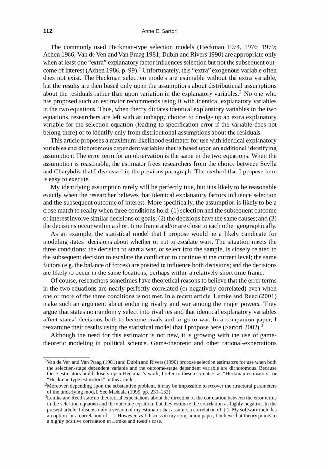
−γ′xi ). Because ui has a standard normal distribution, this probability is just thecumulative standard normal density evaluated at −γ′xi ; this is the area under thecurve to the left of the line at −γ′x in Fig. 1A or 1B. Thus,

Pi0 = �(−γ′xi ). (14)

9The analogous Heckman-type estimator also considers the two equations together.10The likelihood is proportional to the probability of the data (King 1990, p. 22). The maximum of the likelihood

is attained at the same parameter values as the maximum of the probability of the data, and so I replace theproportionality sign with an “equals” sign for the remainder of the paper.

P1: GIB

OJ006-01 March 29, 2003 11:46


(A) (B)

Fig. 1 The distribution of ui when (A) −γ′xi < −β′xi and (B) −β′xi < −γ′xi .

2. j = 1. The observation is selected into the second equation and has an observedoutcome of 0 in that equation. In the equation of interest (6), the outcome is 0 ifβ′xi + ui < 0, or ui < −β′xi . The derivation of Pi1 requires two steps:

1. Consider an observation and true model for which −β′xi > −γ′xi for the trueparameter values and the observation in question (Fig. 1A). In the usual probitsetup, the probability of a 0 would be �(−β′xi ), represented by the area to the leftof the line at −β′x in Fig. 1A. However, the observations for which ui < −γ′xi

did not make it into the sample. Thus, the ex ante probability that a 0 is in theequation of interest is �(−β′xi ) − �(−γ′xi ). This is the probability representedby the region of Fig. 1A between the two vertical lines.

2. Now consider an observation and model for which −β′xi ≤ −γ′xi (Fig. 1B). Inthis case, one cannot observe Yi1 = 1. To see this, suppose that the error termfor the observation is such that ui < −β′xi . Then ui < −γ′xi also. Thus, anyobservation that would have an outcome of 0 in the second stage is not selectedinto the sample for that stage. Thus,

Pi1 ={

�(−β′xi ) − �(−γ′xi ) if (γ′ − β′)xi > 0

0 if (γ′ − β′)xi ≤ 0.(15)

When the observed Yi1 equals 1, −β′xi ≤ −γ′xi leads to a contradiction; theprobability of an existing observation cannot be 0. If an observation is selected intothe second equation and has an outcome of 0 in that equation, it therefore must bethat −β′xi > −γ′xi for that observation at the true values of the parameters.

3. j = 2. The observation is selected into the second equation and has an observedoutcome of 1 in that equation. In the equation of interest (6), the outcome is 1 ifβ′xi + ui > 0, or ui > −β′xi . The derivation of Pi2 also takes two steps:

1. If −β′xi > −γ′xi (Fig. 1A), then any observation for which β′xi + ui > 0has a value of 1 on the observed dependent variable. The probability of such anoccurrence is 1 − �(−β′xi ), or �(β′xi ).

2. If −β′xi ≤ −γ′xi (Fig. 1B), then not all observations for which ui > −β′xi arein the sample for the second stage. In this situation, only when ui > −γ′xi doesone observe a 1 in the dependent variable of interest. Thus, the probability of a 1in the second-stage is 1 − �(−γ′xi ), or �(γ′xi ).

P1: GIB

OJ006-01 March 29, 2003 11:46

120 Anne E. Sartori

Thus,

Pi2 ={

�(β′xi ) if (γ′ − β′)xi > 0

�(γ′xi ) if (γ′ − β′)xi ≤ 0.(16)

If −β′xi < −γ′xi , then the second version of Pi2 will be smaller; if the reverse is true, thefirst version will be smaller, and so in practice,

Pi2 = min[�(γ′xi ), �(β′xi )]. (17)

I distinguish the two probabilities by subscript because I use them separately in the proofs:

Pi21 = �(β′xi ); (18)

Pi22 = �(γ′xi ).

Having calculated the probabilities that enter into the likelihood function, I now definethe estimator:

β, γ:= maxβ,γ∈Θ

L∗, (19)

where θ is the vector of all parameters and Θ is the parameter space.11 The variance–covariance matrix of the estimators is estimated by:

(−∂2L(θ)

∂θ∂θ′

)−1

(20)

(Greene 1993, p. 115).The estimates never imply that an observed outcome is impossible. However, depending

upon the data, they may imply that an outcome that never is observed is impossible. Inother words, they may imply that if an observation with certain values of the independentvariables xi selects in, then that observation always obtains a value of 1 for the observeddependent variable in the outcome equation (never has the outcome Yi1 = 1). This is mostlikely for values of xi outside the defined or usual ranges of the independent variables.12

4 Experimental Comparison of Probit, Heckman, and Sartori Estimators

In this section, I use Monte Carlo simulations to investigate the conditions under whichmy estimator is an improvement over the Heckman estimator and over ordinary probit. Thesimulations vary the “real” situation in order to evaluate the performance of each estimatorunder different conditions, all of which include nonrandom selection.

11The possible presence of a zero or negative probability in the likelihood (from Pi1) when the parameters arenot equal to their true values can pose a problem for estimation using a numerical search routine since the loglikelihood is undefined for these probabilities. The software surmounts this problem by replacing the zero ornegative number in the likelihood function with a “punishment” variable that moves the optimization routineaway from guesses that are impossible. It also confirms that the final estimates are in the feasible range.

12It might be possible to modify the computer program to restrict the estimates to values that imply that alloutcomes are possible within the plausible ranges of the independent variables.

P1: GIB

OJ006-01 March 29, 2003 11:46


As I discussed earlier, scholars have two main reactions when theory implies that iden-tical explanatory factors influence selection and the subsequent outcome of interest. Someestimate with identical explanatory variables, whereas others add an exclusion restriction.I thus perform two sets of simulations. In the first and primary set of simulations, I eval-uate the three estimators, assuming that identical explanatory factors influence selectionand the subsequent outcome of interest (the situation for which my estimator is intended).In the second set of simulations, I evaluate them assuming that there is a valid but weakexclusion restriction. Note that if identical explanatory factors truly do influence selec-tion and the subsequent outcome of interest, a valid exclusion restriction simply does notexist. My second set of simulations is based on the idea that the researcher, through addi-tional thought, might come to the conclusion that his/her original theory was incomplete,and that selection and the subsequent outcome of interest do not after all have identicalcauses.

In each experiment, I estimate 1000 times using each of the three estimators.13 To createthe data sets, I begin by creating an explanatory variable, x . I use two samples, one with100 and one with 1000 observations. I do so by drawing 1000 observations from a normaldistribution with mean 0 and variance 0.64. I set the variance of the explanatory variableat 0.64 so that the systematic component of the selection mechanism will have the samevariance as the error term; in other words, the systematic component and the error areequally important in the selection equation. (Later, I report results from simulations thatvary the ratio of the systematic component to the error.) I take the first 100 observationsas my sample of 100 and the entire data set as my sample of 1000. The realized mean forthe first 100 observations of the independent variable is 0.135 and the standard deviationis 0.6464. The realized mean for the whole sample of 1000 is 0.0385 and the standarddeviation is 0.63264.

Next, for each experiment, I generate 1000 samples of the dependent variable. As Idescribe later, in each sample, the dependent variable is a function of the explanatoryvariable (the 100 or 1000 observations of x) and of new draws of the error terms. In otherwords, the data-generating process has a systematic component and a random component.

Because ordinary probit gives consistent estimates of the selection-equation parameters,I discuss only the estimates for the outcome equation. In the interests of brevity, I discussonly the slope estimates; I also consider only one criterion, the root mean square error, forevaluating the simulations with a weak exclusion restriction.

4.1 Simulations with Identical Explanatory Variables

In the simulations with identical explanatory variables, I create the underlying utilities andthe dichotomous dependent variables as follows:

U1 = 1.25 ∗ x + u1 (21)

U2 = −0.7 + 1.5 ∗ x + u2. (22)

Here, U1 represents the actor’s utility from “selecting in” and U2 represents its utility from“going on,” or getting a 1 in the outcome equation. As is usual in probit-style models, oneobserves a dichotomous dependent variable instead of the underlying utility. One observes

13I conduct all of the simulations in STATA using STATA’s heckprob and probit commands and the program thatimplements my estimator.

P1: GIB

OJ006-01 March 29, 2003 11:46

122 Anne E. Sartori

Table 1 Mean bias (β2 = 1.5) (numbers rounded)

ρ Probit Heckman Sartori

100 observations.9 −.181 −.212 .102.5 −.0657 −.164 .159.1 .105 −.0647 .294

1000 observations.9 −.314 −.217 −.00693.5 −.227 −.157 .0478.1 −.0437 −.0859 .176

Y1 = 1 if U1 > 0; Y1 = 0 otherwise, and Y2 = 1 if U1 > 0; Y2 = 0 otherwise. In theanalyses that follow, I refer to the intercept and slope in the selection equation (21) as α1

and β1, respectively, and those from the outcome equation (22) as α2 and β2, respectively.The Heckman estimator’s key identifying assumption is that the errors in the selec-

tion equation and the outcome equation are jointly normally distributed. In practice, theresearcher often does not know to what extent this assumption accurately represents thedata-generating process. For this reason, one purpose of the simulations was to evaluatethe performance of each estimator with a variety of error-term distributions. However, itturns out that the Heckman estimates are quite poor when there is no valid exclusion re-striction, even when the estimator’s key identifying assumption is met.14 Thus, this articlediscusses only the simulations with error terms (us) that are drawn from a bivariate normaldistribution.

My estimator’s key identifying assumption is that the errors from the two equationshave a correlation of 1 (or of −1, depending upon the choice of the user).15 In practice,the researcher may know from theory that the errors are highly correlated, but is unlikelyto know that the correlation is 1. Thus, a second goal of the simulations was to vary thetrue correlation between the errors and to evaluate the performance of each estimator. Iconsider situations in which the true correlation (ρ) between u1 and u2 is .9 (my estimator’sassumption is close to true). I then consider situations in which the true ρ is only .5 (theassumption is fairly far from true) and .1 (the assumption is quite far from true). Later, Ireport results from simulations in which the true ρ is −.1, −.5, and −.9.

I evaluate the coefficient estimates and the standard-error estimates produced by eachof the estimators using three criteria: the mean bias of the estimates (MB), the root meansquare error (RMSE) of the estimates around the true parameter, and the coverage.16 Themean bias is information about the average result: insofar as the estimates differ from thetruth, to what extent do positive errors and negative errors cancel each other out? The RMSEis the average variability of the point estimate around the true parameter. The RMSE differsfrom the sampling variability, which is variation around the sample mean of the estimate,rather than around the true parameter. For example, the RMSE of the probit estimate of

14Some results from simulations with modified t and chi-square errors are available on the Political Analysis Website.

15In the simulations, I use the version of my estimator that assumes that the correlation between the errors is +1.My estimator also assumes that the errors are normally distributed.

16The mean bias is the bias divided by the number of replications in which the estimates in question converged.

P1: GIB

OJ006-01 March 29, 2003 11:46


Fig. 2 RMSEs of estimates of β2, 1000 observations.

β2 is√∑

i (βPi2−β2)2

n , where β2 is the true value, βPi2 is the probit estimate of β2 in the i th

replication, and n is the number of estimates.17

The coverage is information about the combined accuracy of the coefficient estimatesand the standard error estimates. I compute the 95% confidence interval for each replicationof the simulation using the estimate of β2 and the estimate of its standard error. The coverageis the frequency with which these confidence intervals contain the true value of β2. Ideally,one would like the 95% confidence interval to contain the true value 95% of the time.

In calculating these summary statistics, the issue arises of how to treat replications inwhich one or more estimators did not converge. Only probit converged in every replication.For example, with 100 observations, Heckman converged 912/1000 times with a true ρ of.9 and 907/1000 times with a true ρ of .5. With the same sample, my estimator converged922/1000 times with a true ρ of .9 and 943/1000 times with a true ρ of .5. In the statisticsthat follow, the numbers reported are averages over the replications that did converge.I would speculate that the Heckman estimator and my estimator are failing to convergewhen estimation is difficult, and that the nonconvergence results should be considered badestimates. (If the estimates had converged in replication j , they would have been far fromthe truth.) If so, my estimator probably performs better relative to the Heckman estimatorthan I report below in most of the simulations (because it converges more frequently), butboth selection estimators perform worse in relation to ordinary probit.18

4.1.1 Coefficient Estimates: Mean Bias and RMSEs

The striking result of the simulations is that my estimator performs better than Heckman’s,even when Heckman estimator’s key assumption about functional form is met, and myestimator’s assumption of identical errors is fairly far from the truth. Table 1 and Fig. 2

17The number of estimates is not 1000 for every estimator and simulation because the Heckman estimator and mynew estimator did not always converge.

18However, one might prefer a result of nonconvergence to an inaccurate estimate, because one has no way ofknowing which estimates are inaccurate.

P1: GIB

OJ006-01 March 29, 2003 11:46

124 Anne E. Sartori

Table 2 Mean bias, new sample of 100 observations(β2 = 1.5) (numbers rounded)


.9 −.218 −.320 .0743

.5 −.120 −.287 .123

.1 .114 −.229 .305

show the mean bias and the RMSE of the slope coefficient in the outcome equation. In allthe simulations that the table and the figure summarize, Heckman’s key assumption is met.In none of these simulations is my estimator’s key assumption met—the highest correlationin the simulations is .9, whereas my estimator assumes a correlation of 1.0.

Despite the Heckman estimator having this advantage, the Heckman estimates of theslope coefficient have greater mean bias than my estimates, even when my estimator’sassumption is fairly far from the truth—the true ρ is only .5. Only when there is almost noselection bias (the true ρ is .1), does Heckman estimator have less bias than my estimator.Moreover, when the true correlation is this low, ordinary probit outperforms the Heckmanestimator in the simulation with 1000 observations.19 The magnitudes of the biases aresmall but not negligible; for example, the Heckman estimator’s bias of −.217 when thetrue ρ is .9 and the sample size is 1000 corresponds to about 15% of the magnitude ofthe coefficient. Of course, the direction of the bias also matters. With the sample of 100observations, my estimator’s average bias would overstate the effect of the independentvariable, whereas Heckman’s would understate it. With the sample of 1000 observationsand correlations of .5 and .9, my estimator has only trivial bias, making the direction of thebias almost inconsequential.

The results from the simulations with 100 observations are somewhat peculiar. Becauseordinary probit is consistent when the errors in the selection equation and the outcomeequation are uncorrelated, I would expect probit to do worse at high (in absolute value)values of ρ. In this set of simulations, however, the ordinary probit estimates have lessaverage bias when the true correlation between the errors is .5 than they do when the truecorrelation is .1. This result is probably an artifact of the particular small sample of theexplanatory variable used in the simulations. Table 2 shows results of simulations that use adifferent sample of 100 observations of the explanatory variable.20 Using this second set ofdata, probit has lower mean bias when ρ is lower.

My estimator has a smaller RMSE for the outcome-equation estimates than either ofthe other estimators in every simulation shown in the figure—regardless of whether thesample has 100 or 1000 observations, and, more surprisingly, of whether the true ρ is .9, .5,or .1. The impact of the Heckman estimator’s RMSE when the independent variables areidentical is again not trivial. Even with samples of 1000 observations, the Heckman estima-tor’s RMSE is more than a fifth of the true slope. With 1000 observations, my estimator’sRMSE for β2 is only 23% or 31% that of Heckman’s, depending upon the true correlationbetween the error terms.

19With this sample of 100 and a ρ of .5, ordinary probit has lower mean bias than either of the other two estimators.However, my estimator has lower RMSE and more-accurate coverage.

20The new sample of the explanatory variable is drawn from the same distribution as the previous one; the realizedmean of the explanatory variable is −0.069. I create 1000 samples on which to estimate the parameters in thesame way as before, by taking new draws of the error terms.

P1: GIB

OJ006-01 March 29, 2003 11:46


Table 3 Coverage, 95% confidence interval(numbers rounded)


100 observations.9 .873 .828 .933.5 .905 .856 .934.1 .952 .836 .931

1000 observations.9 .253 .868 .948.5 .499 .889 .919.1 .930 .797 .599

In sum, the coefficient estimates in the simulations suggest that my estimator is bettersuited to the problem of identical explanatory variables than is the Heckman one. Myestimates have lower mean bias and RMSE around the true coefficient than Heckman’s, evenwhen the assumption of identical errors is fairly far from true and Heckman’s assumptionof normally distributed errors is true. In very small samples, however, my estimator, onaverage, leads to overstating the impact of the explanatory variable whereas the Heckmanestimator leads to understating them. I next investigate the coverage, because this may affectthe conclusions the researcher draws from the estimates of the coefficients.

4.1.2 Inference: Coverage

When identical explanatory variables influence selection and the outcome of interest, mynew estimator also results in more accurate inference than the Heckman estimator, evenwhen the Heckman estimator’s key assumption is met and my estimator’s assumption ofidentical errors is fairly far from the truth. As Table 3 shows, my estimator’s 95% confidenceinterval is closer to accurate when the true ρ between the errors is .9 or .5. When the truecorrelation is .1 (there is almost no selection bias) and the sample size is 1000, Heckman’sconfidence interval is more accurate than mine, but probit’s is the most accurate of all.

4.1.3 The Heckman Estimator’s Estimates of ρ

The Heckman estimator is the only one of the three procedures that yields an estimate ofthe correlation between the error terms in the two equations, ρ. This is an advantage—ingeneral, one would rather estimate a parameter than assume its value. However, whenidentical explanatory variables belong in the selection equation and the outcome equation,Heckman estimator’s estimate of ρ is often extremely misleading, as Table 4 and Figs. 3Aand B show. In some of the simulations, such as the simulation with 1000 observationsshown in the figure, there is a relatively high frequency of estimates that are 1 or very closeto 1, regardless of whether the true ρ is .9 or .5. The distribution of ρ has a spike just shy of 1;

Table 4 RMSEs of Heckprob’s estimates of ρ

True ρ 100 observations 1000 observations

.9 1.02 .784

.5 .826 .582

.1 .788 .586

P1: GIB

OJ006-01 March 29, 2003 11:46

126 Anne E. Sartori

(A) (B)

Fig. 3 Histogram of Heckman’s estimates of ρ: true ρ is (A) .9 and (B) .5.

this spike need not occur around the truth, since it also appears when the true ρ is .5. Asidefrom those two areas of higher probability, the distribution is fairly flat. Thus, the fact that theHeckman procedure provides estimates of ρ is not an advantage when identical explanatoryfactors influence selection and the outcome and one has strong prior beliefs about ρ.

4.1.4 At What True Values of ρ is Each Estimator Best?

The figures and tables above show that my estimator is a better choice for this problemthan the Heckman-type ones, even when the true ρ between the errors is as low as .5. Myestimator allows one to assume that the true correlation between the errors is +1 or −1. Inthe simulations, I use the version of the estimator that assumes a correlation of positive one.As one would expect, the tables and figures mentioned above show that this version of myestimator performs better when the true correlation is higher.

Figure 4 draws out this pattern further. The figure examines the RMSE of the slopecoefficient in the outcome equation for a greater range of true correlations of the error term.In each of these simulations, the errors are normally distributed and the sample size is 1000.

Fig. 4 RMSEs of estimates of β2.

P1: GIB

OJ006-01 March 29, 2003 11:46


The figure shows more clearly that my estimator does best when its assumption is closestto true. My estimate has lower RMSE than Heckman’s in each simulation in this set exceptthe simulation with a true ρ of −.5.21 However, when the true ρ between the errors is smallin magnitude (.1 or −.1 in these simulations), ordinary probit has lower RMSE than eitherof the selection estimators.

The mean bias of my estimates is lower than that of Heckman’s at high correlationsand becomes higher than Heckman’s as the correlation moves toward zero. In the samplewith 1000 observations, the switch occurs somewhere between a true ρ of .3, where myestimates have a smaller mean bias, and one of .2, where Heckman’s have a smaller meanbias. Similarly, my estimator’s coverage is more accurate at high correlations and becomesless accurate at low correlations. In the sample with 1000 observations, the switch occurssomewhere between a true ρ of .4, where my estimator’s coverage is more accurate, and.3, where Heckman’s coverage is more accurate. At very low correlations, probit has thelowest bias and most-accurate coverage.

The right choice when identical explanatory variables belong in the two equations thusdepends upon the guidance that theory provides about the sign and size of the correlation.Probit is the right choice if the errors are largely unrelated. My estimator is the right choiceif the correlation between the errors is high and of a specific sign, either positive or negative.Finally, the Heckman estimator is the best choice if the errors are highly correlated (makingprobit undesirable), but the researcher is quite uncertain about the true sign of the correlation(making my estimator undesirable). Even under these very limited circumstances, Heckmanestimates are not good, they are just better than those of the other estimators. Since Heckmanestimates of ρ are often very far from the truth (see above), the choice of estimators mustbe made largely on theory rather than on the basis of those estimates.

4.1.5 Do the Results Change if the Systematic Component Is More/LessImportant Relative to the Error Term?

In the simulations I discussed earlier, the systematic component and the error term in theselection equation are equally important. One might expect ordinary probit to perform betterin relation to both Heckman and my estimator when the error term is less important. Thisis because the inconsistency of probit (“selection bias”) is due, in part, to the fact that theobservations’ error terms affect their probabilities of selecting into the sample. To assessthe sensitivity of my conclusions to the relative importance of the error term, I performadditional simulations. These are identical to those I described earlier, except that I vary theratio of the variance of the systematic component to that of the error term in the selectionequation [var(β1x)/var(u)].22 The RMSEs reveal the same general pattern as before: Myestimator performs better than Heckman’s and probit when the errors are highly correlated.Probit performs better than both selection estimators when the correlation between theerrors is very low.

As expected, probit tends to perform better in absolute terms when the systematic com-ponent is more important relative to the error term. However, it does not perform betterrelative to the other two estimators. This is because all the estimators tend to perform betterwhen the systematic component is more important; a more important systematic component

21I did not investigate correlations between −.1 and −.5. The Heckman estimator probably begins to outperformmine when the correlation is between those values.

22I do this by changing the variance of the explanatory variable. The values of the ratio var(β1x)var(u) in the table are

based on the theoretical variance of x rather than its sample variance.

P1: GIB

OJ006-01 March 29, 2003 11:46

128 Anne E. Sartori

Table 5 RMSEs of β2, ρ = .5, varying the relativeimportance of the systematic component and the error

var(β1x)var(u) Probit Heckman Sartori

0.1 .374 .910 .2100.5 .283 .461 .1151 .258 .337 .1052 .241 .275 .00994

10 .234 .260 .119

means more information and less noise for the estimators to work with. As an example,Table 5 shows the results of varying var(β1x)

var(u) when the true ρ is .5 and the sample size is 1000.There are two surprising results. First, the Heckman estimator performs especially badlyin comparison to the others when there is very little information [ var(β1x)

var(u) = .1]. Second,although all of the estimators improve in RMSE as the importance of the systematic com-ponent increases, my estimator does worse when the ratio of the variance of the systematiccomponent to that of the error is very high (10:1), than when it is moderately high (2:1).At even higher ratios of var(β1x)

var(u) (not shown), the RMSEs of probit and the Heckman-typeestimator also begin to increase.

4.2 Simulations with an Exclusion Restriction

When theory points to identical explanatory factors, a common response is a mad search foran exclusion restriction.23 This practice is dangerous because including the “extra” variablemay lead to specification error. For example, if the extra variable does not affect selectionin the population but is correlated with a true explanatory variable and with selection in thesample, including it in the equation can bias the estimates of the effect of the explanatoryvariable.

This section of the article assumes a best-case scenario for a weak exclusion restriction:the dredged up explanatory variable (z) actually does influence selection and is uncorrelatedwith the explanatory variable of interest. I investigate the RMSEs of the slope coefficient(β2) in the outcome equation for each of the estimators under this scenario, using a samplesize of 1000 and errors from a bivariate standard normal distribution with correlation .9, .5,or .1. I create the “extra” variable that enters the selection equation, z, by taking 1000 drawsfrom a uniform normal distribution, independent of the distribution of the other explanatoryvariable, x. I examine two cases: one in which the true coefficient on z is small (.05), andone in which the true coefficient is larger (.25).24 The small coefficient corresponds to a“weak” exclusion restriction, whereas the larger one corresponds to a stronger restriction.When I estimate with ordinary probit or with the Heckman estimator, I include z in themodel. However, when I use my estimator, I estimate only with x.

For the weaker exclusion restriction, I choose the magnitude of the coefficient (c) onthe extra variable (z) to obtain a t-statistic of just over 1, on average, for the Heckmanestimates. My reasoning is that a researcher finding a t-statistic of that size might believe

23If there is a valid and significant exclusion restriction, then the Heckman estimator is the best choice. Bydefinition, however, there is no valid exclusion restriction if selection and the subsequent outcome truly haveidentical causes.

24Note that the extra variable z has higher variance than the original explanatory variable x , so that its coefficientis not immediately comparable to the coefficient on x .

P1: GIB

OJ006-01 March 29, 2003 11:46


Fig. 5 RMSEs of β2 when a very weak exclusion restriction is valid.

himself or herself to have a valid, though weak, exclusion restriction.25 With the weakexclusion restriction, moving from one standard deviation below the mean of z to onestandard deviation above (with x at its mean) leads to a true increase of about 4 percentagepoints in the probability of selecting into the sample.

For the stronger exclusion restriction, I choose the magnitude of the coefficient on theextra variable to obtain a t-statistic of over 5, on average, for the Heckman estimates. Movingfrom one standard deviation below the mean of z to one standard deviation above, againwith x at its mean, leads to an increase of almost 20 percentage points in the probability ofselecting into the sample.

Figure 5 shows the RMSEs of the slope coefficients in the outcome equation when theweaker exclusion restriction is valid. The figure demonstrates that the weaker exclusionrestriction is a poor assistant to the Heckman model. Heckman estimator’s RMSEs arevery similar to what they were for the model without a valid exclusion restriction. Myestimator’s RMSEs are also very similar, and remain much smaller than Heckman’s in allof the simulations.26 As in the previous simulations, my estimator outperforms probit in thesimulations where the true ρ between the errors is .5 or .9, and underperforms probit whenthe true ρ is .1.

The stronger exclusion restriction is more of a help to the Heckman model, but it isnot a savior. When the true ρ between the errors is .5 or .9 and the extra variable reallyis explanatory, the Heckman estimator now does considerably better than ordinary probit,which it did not before (see Fig. 6). However, my estimator still has lower RMSEs than theHeckman estimator for all three correlations (.9, .5, and .1), even though I used an incorrectspecification for my estimates, because the extra variable does influence selection in thisset of simulations.

Clearly, the Heckman estimator will outperform mine when the extra variable has alarge enough effect (and truly is explanatory). However, as these simulations show, largeenough is not a trivial requirement. In this example, varying the more-important “extra”explanatory variable from a standard deviation below its mean to a standard deviation above

25Of course, t-statistics vary with sample size.26I do not examine here situations in which the true correlation is highly negative and I assume it to be highly

positive. The Heckman estimator would surely outperform mine in such a simulation, as it did without theexclusion restriction.

P1: GIB

OJ006-01 March 29, 2003 11:46

130 Anne E. Sartori

Fig. 6 RMSEs of β2 when a stronger (but still weak) exclusion restriction is vaild.

results in a 20 percentage point increase in the probability of selection, but the Heckmanestimator’s RMSEs are still larger than mine. If a researcher grubs up a variable simplyto get an exclusion restriction, chances are that this variable will not be important enoughto make Heckman estimates the better choice, even if the variable is actually related toselection. If theory truly indicates that at least one variable has a reasonably large effect onselection but not on the subsequent dependent variable, then the Heckman estimates indeedare likely to be better.

5 Does it Matter?

Does the choice of estimators for this problem affect the conclusions one reaches whenanalyzing real data? In a companion paper, I show that the answer is “yes” for one importantsubstantive example (Sartori 2002). Lemke and Reed (2001) use the Heckman estimatorto examine the causes of war among enduring rivals, arguing that identical explanatoryvariables influence the decision to become rivals and the decision to go to war. Their resultscontradict all of the findings in the existing literature on the causes of war among rivalsthat they consider.27 I argue that there are good theoretical reasons to believe that ρ in theircase is large and positive. Using my estimator, I obtain estimates that are almost entirelycontrary to those of Lemke and Reed on the causes of war among rivals and are consistentwith the previous literature.

6 Conclusion

This article provides a consistent, asymptotically normal, maximum-likelihood estimator foruse in selection models when the same set of independent variables affect both the selectionequation and the equation of interest and when both dependent variables are binary. Theestimator identifies from an assumption that the error terms in the selection equation andthe outcome equation are identical for a given observation. It fills a need in quantitativepolitical science research because nonrandom selection is ubiquitous and because the ex-isting, Heckman-type models are best used only with an exclusion restriction—when the

27Lemke and Reed’s results do not contradict the findings in the existing literature they consider on the causes ofrivalry.

P1: GIB

OJ006-01 March 29, 2003 11:46


researcher believes that at least one variable that influences selection does not influence thesubsequent process of interest. In many substantively interesting problems, the same factorsaffect both processes. The new estimator’s identifying assumption is likely to be reasonableunder exactly this circumstance. When the assumption is reasonable, as long as both depen-dent variables are binary, this model avoids the unfortunate choice among identifying fromfunctional form alone, adding a theoretically unjustified variable in a mistaken attempt to“boost” identification, and giving up on estimation entirely.

The simulations confirm that this estimator is a better solution to the problem of identicalexplanatory factors than either of the common alternatives for estimation—identifying fromfunctional form alone or adding an “extra” variable to the selection equation when one isskeptical that it belongs there. First, this estimator is a better choice than the Heckmanestimator when identical explanatory variables affect selection and the dependent variableof interest and the sample size is small. The proposed estimator has lower mean bias andlower mean square error for the slope estimates in the equation of interest—not only whenits own identifying assumption is close to being met, but also when its assumption is fairlyfar from the truth (the true ρ is only .5) and Heckman’s identifying assumption is met. It alsoprovides more accurate 95% confidence intervals, thus decreasing the chances of incorrectinference. Second, dredging up an exclusion restriction is a poor solution to this problem.Even if the added variable actually does belong in the equation, that variable must havequite a large effect on selection for the Heckman estimates to have lower RMSE than mine.

As sample size approaches infinity, and if the errors truly are normally distributed, theHeckman estimator is the best choice. It is consistent and identified, though its identificationis weak. In small samples, it does not have the information needed to distinguish betweenthe effects it is trying to estimate; very large samples provide the needed information.

The choice of estimators with small-to-medium samples should depend on politicaltheory. When theory points to identical explanatory variables but very little selection bias,ordinary probit is the best choice of the three estimators. When theory suggests identicalexplanatory variables and a high degree of selection bias, but not the sign of the correlationbetween the errors (a situation likely to be rare), the Heckman estimator is the best choice,although still a poor option. However, when theory points to identical explanatory variablesand implies that the errors are correlated in a particular direction, the new estimator givesconsiderably better results than either probit or the Heckman-type estimator. The newestimator is therefore a badly needed tool for applied researchers who believe that identicalexplanatory variables influence selection and a later binary dependent variable of interest.

Appendix: Proofs

Maximum-likelihood estimators usually have several nice properties: consistency, asymp-totic normality, and asymptotic efficiency. However, not every maximum-likelihood estima-tor has these properties (Amemiya 1985, ch. 4). In this appendix, I prove that the estimatorderived in this article is consistent and asymptotically normal. Asymptotic efficiency fol-lows from asymptotic normality (Amemiya 1985, p. 123). My proofs build on proofs of theconsistency and asymptotic normality of the parameter estimates in a probit model givenby Amemiya (1985, pp. 271–273).

Notation: Let γ0 and β0 be the true parameter values, Pi j or Pi jk be the probability thatYi jk = 1 (with k used only when necessary to clarify the distinction between Pi21 and Pi22),Pi jk0 be the value of Pi jk at the true values of the parameters, θ be the set {γ, β}, θ0 be theset {γ0, β0}, and xi be a row vector containing the values of the explanatory variables forobservation i .

P1: GIB

OJ006-01 March 29, 2003 11:46

132 Anne E. Sartori

A.1 Consistency

I make three assumptions about the model:

Assumption 1. The parameter space Θ is an open-bounded subset of Euclidian K -space.

Assumption 2. {xi } are uniformly bounded in i and limn→∞ n−1 ∑ni=1 x′

i xi is a finite non-singular matrix. The empirical distribution of {xi } converges to a distribution function.

Assumption 3. prob(β′0xi = γ′

0xi ) = 0.

The statement in Assumption 3 is true as long as at least one independent variableis continuous without any mass points and β0 �= γ0. Alternatively, it may be true due tobounds on the independent variables. If all independent variables are dichotomous, thestatement restricts the applicability of the model to data-generating processes that meet theassumption.

That the statement is ever true without assumption is not intuitive, because the equationβ′

0xi = γ′0xi has an infinite number of solutions as long as it contains more than one

independent variable. It is true for continuous x without mass points for the followingreason. The equation in the assumption defines a hyperplane. If there are k independentvariables (xs), the hyperplane has dimension k − 1. The space of xs over which solutionsmight be found has k dimensions. Thus, the probability of finding a solution is zero eventhough the number of solutions is infinite.

Theorem 1. Given Assumptions 1–3, β and γ as defined in (19) are consistent estimatesof γ0 and β0.28

Proof: I prove three lemmas that lead to the theorem.Without loss of generality, I divide the data into two parts. The first part, observations

i = 1, . . . , m, consists of observations such that �(−β′xi ) > �(−γ′xi ). The second part,observations i = m + 1, . . . , n, consists of observations such that �(−β′xi ) ≤ �(−γ′xi ).I now make a fourth assumption about the model.

Assumption 4. The number of observations m and the number n − m go to infinity at thesame rate as n. The fractions m

n and n−mn converge to fractions µ1 and µ2, where 0 < µ1 ≤ 1

and 0 ≤ µ2 < 1.Let Qn(y, θ) ≡ L∗. Then, from the text,

Qn(y, θ) =n∑

i=1

Yi0 ln �(−γ′xi ) +m∑

i=1

Yi1 ln[�(γ′xi ) − �(β′xi )]

+m∑

i=1

Yi2 ln �(β′xi ) +n∑

i=m+1

Yi2 ln �(γ′xi ).

28The theorem that I use (4.1.2 in Amemiya 1985) is a standard theorem for proving consistency; for example,Amemiya uses it to show consistency of the estimates obtained through probit estimation (Amemiya 1985,pp. 270–273). Technically, the theorem states that one of the local maxima is consistent and does not specifywhich one if there are multiple local maxima (Amemiya 1985, p. 111). However, as long as Q(θ) (the functionto which n−1 L∗ converges in probability in the proofs below) has a unique global maximum, the conditionsof Theorem 4.1.1 (Amemiya 1985, pp. 106–107) also are met and β and γ as defined in (19) are consistentestimates of γ0 and β0.

P1: GIB

OJ006-01 March 29, 2003 11:46


Lemma 1. ∂Qn(y, θ)/∂θ exists and is continuous in an open neighborhood N1(θ0)of θ0.

Proof: This lemma follows from the normality of the cumulative densities in Pi j . Thepartial derivatives of the likelihood are not continuous at �(β′xi ) = �(γ′xi ). Such an eventhas probability of 0 in an open neighborhood of the true parameters by Assumption 3 andthus does not affect consistency (Huber 1967; Pakes and Pollard 1989). �

Lemma 2. Let gi jk(y, θ) ≡ (Yi j − Pi jk0) ln Pi jk . Then n−1 ∑ni=1 gi0(y, θ) converges

to 0; m−1 ∑mi=1 gi1(y, θ) converges to 0; m−1 ∑m

i=1 gi21(y, θ) converges to 0; and (n −m)−1 ∑n

i=m+1 gi22(y, θ) converges to 0. In addition, there exists an open neighborhood ofthe two parameter vectors, N2(θ0), such that n−1 Qn(y, θ) converges to a nonstochasticfunction Q(θ), where

Q(θ) = limn→∞ n−1

n∑i=1

Pi00 ln Pi0 + limm→∞

m

nm−1

m∑i=1

(Pi10 ln Pi1 + Pi210 ln Pi21)

+ lim(n−m)→∞

n − m

n(n − m)−1

n∑i=m+1

Pi220 ln Pi22. (A1)

Proof:

1. The normality of the cumulative densities in Pi j and Assumptions 1–3 imply thatgi jk(y, θ) satisfies the conditions for gt in Theorem 4.2.2 in Amemiya (1985, p. 117)in a compact neighborhood of θ0.

2. By Theorem 4.2.3 in Amemiya (1985, p. 118), the limits in Q(θ) exist.

3. By Theorem 4.2.2, n−1 ∑ni=1 gi0(y, θ), m−1 ∑m

i=1 gi1(y, θ), m−1 ∑mi=1 gi21(y, θ),

and (n−m)−1 ∑ni=m+1 gi22(y, θ) converge uniformly to 0 in probability when θ ∈ Θ.

4. By the previous step, n−1 ∑ni=1 Yi0 ln Pi0 − n−1 ∑n

i=1 Pi00 ln Pi0 converges to 0, sothat n−1 ∑n

i=1 Yi0 ln Pi0 converges uniformly to n−1 ∑ni=1 Pi00 ln Pi0 in probability

when (β, γ) ∈ N (β0, γ0), an open neighborhood of θ0.

Analogous reasoning applies to the other terms in the empirical likelihood. Alongwith Assumption 4, Steps 1–4 imply that n−1 Qn(y, θ) converges to Q(θ). �

Lemma 3. Q(θ) attains a strict local maximum at β0, γ0.

Proof: I first differentiate Q(θ) in an open neighborhood of the true parameter values toshow that a critical point occurs at β0, γ0. The assumptions allow differentiation insidethe limit operation (Amemiya 1985, p. 271). Without loss of generality, I again divide thedata into two parts. The first part, observations i = 1, . . . , m, consists of observations suchthat �(−β′

0xi ) > �(−γ′0xi ). The second part, observations i = m + 1, . . . , n, consists

of observations such that �(−β′0xi ) ≤ �(−γ′

0xi ). The proof is easier to follow with ab-breviated notation. For example, let Fiβ0 represent the cumulative density of the normaldistribution evaluated at β′

0xi and fiβ0 be its first derivative. Fiβ is the cumulative nor-mal evaluated at β′xi , where β need not be the true value, and fiβ is its first derivative.

P1: GIB

OJ006-01 March 29, 2003 11:46

134 Anne E. Sartori

Then,

∂Q

∂β= ∂

∂βlim

n→∞ n−1

(m∑

i=1

[(1 − Fiγ0) ln (1 − Fiγ) + (Fiγ0 − Fiβ0) ln (Fiγ − Fiβ)

+ Fiβ0 ln Fiβ] +n∑

i=m+1

[(1 − Fiγ0) ln (1 − Fiγ) + Fiγ0 ln Fiγ]

)

= limn→∞ n−1

m∑i=1

[−(Fiγ0 − Fiβ0)

Fiγ − Fiβfiβx+ Fiβ0

Fiβfiβx

].

Note that for observations i = 1, . . . , m, ln(Fiγ − Fiβ) is always strictly positive and thusis always defined. At β = β0 and γ = γ

0, the numerator and denominator of each fraction

in the summation sign cancel to 1. Thus, ∂Q∂β

= 0 at β = β0 and γ = γ0.

A similar exercise shows that ∂Q∂γ

= 0 at β = β0 and γ = γ0. Thus, β0, γ0 is a critical

point of Q.Next, I show that Q attains a strict local maximum at β0, γ0. The Hessian of Q is

H =

∂2 Q∂β2

1· · · ∂2 Q

∂βc∂β1

∂2 Q∂γ1∂β1

· · · ∂2 Q∂γc∂β1

.... . .

...∂2 Q

∂β1∂βc

∂2 Q∂β2

c∂2 Q

∂β1∂γ1

∂2 Q∂γ2

1

.... . .

∂2 Q∂β1∂γc

· · · ∂2 Q∂γ1∂γc

· · · ∂2 Q∂γ2

c

(A2)

where c is the number of independent variables. At the true values of the parameters, eachof the second partials with respect to β j , βk or γ j , γk can be written as the same constant(one for the βs and one for the γs) multiplied by xi j xik . For example,

∂2 Q

∂β2j

= − limn→∞ n−1

m∑i=1

Fiγ0

Fiβ0(Fiγ0 − Fiβ0)f 2β0x2

i j

and

∂2 Q

∂β j∂βk= − lim

n→∞ n−1m∑

i=1

Fiγ0

Fiβ0(Fiγ0 − Fiβ0)f 2β0xi j xik,

where j, k denote arbitrary parameters in the vector β.For a given observation i , I could rewrite the Hessian for an observation at the true values

of the parameters as the Kronecker product of two matrices:

(a b

b d

)⊗ x′

i xi . (A3)

The problem with doing so is that the terms in ∂2 Q∂β2 and ∂2 Q

∂γ∂β(a and b above) rely only

upon observations 1, . . . , m. Some terms in ∂2 Q∂γ2 rely on observations 1, . . . , m and others

P1: GIB

OJ006-01 March 29, 2003 11:46


rely upon m + 1, . . . , n. Thus, I divide the Hessian into two parts. H contains the termsinvolving the first set of observations, and H′′ the others. Then,

H = H + H′′. (A4)

To examine the definiteness of H and H′′, let Hi be the Hessian for one arbitrary obser-vation i , where 1 ≤ i ≤ m. Let H′′

i be the Hessian for one arbitrary observation i , wherem + 1 ≤ i ≤ n. Then

Hi =(

a b

b d ′

)⊗ x′

i xi , i ∈ {1, . . . , m} (A5)

and

H′′i =

(0 0

0 d ′′

)⊗ x′

i xi , i ∈ {m + 1, . . . , n}. (A6)

Evaluated at β0, γ0,

a = − Fiγ0

Fiβ0(Fiγ0 − Fiβ0)f 2iβ0, (A7)

b = 1

Fiγ0 − Fiβ0fiβ0 fiγ0, (A8)

d ′ = − 1

1 − Fiγ0f 2iγ0 − 1

Fiγ0 − Fiβ0f 2iγ0, (A9)

and

d ′′ = − 1

1 − Fiγ0f 2iγ0 − 1

Fiγ0f 2iγ0. (A10)

The equations above express Hi and H′′i each as the Kronecker product of two matrices.

To determine the definiteness of H, I first examine H and H′′ separately. The left-handmatrix in Hi is negative definite because a < 0 and ad ′ − b2 > 0. The data matrix ispositive definite.

The definiteness of the two Kronecker-multiplied matrices determines the definiteness ofthe product matrix. The characteristic roots of A⊗B are λiµi , where λi are the characteristicroots of A and µi are the roots of B (Bellman 1960, p. 227). By definition, a matrix is positivedefinite if it has all positive characteristic roots, whereas a matrix is negative definite if ithas all negative characteristic roots (Greene 1993, pp. 35–36). Thus, the Kronecker productof a negative definite matrix and a positive definite matrix is negative definite. Thus, Hi isnegative definite for all i . By similar reasoning, H′′

i is negative semidefinite for all i . (Thefirst component has one zero root and one negative root, while the data matrix again has allpositive roots.)

Note that H = limm→∞ mn

1m

∑mi=1 Hi and H′′ = lim(n−m)→∞ (n−m)

n1

(n−m)

∑ni=m+1 H′′

i .

H is negative definite for the following reason: We have seen that Hi is negative definitefor an arbitrary observation, i . Let Zη = 1

η

∑η

i=1 Hi . Then Zη+1 = η

η+1 Zη + 1η+1 Hη+1.

Multiplying a negative definite matrix by a positive constant results in a negative definite

P1: GIB

OJ006-01 March 29, 2003 11:46

136 Anne E. Sartori

matrix, and adding two negative definite matrices results in a negative definite matrix. ThusH is negative definite. It is also straightforward to show that H′′ is negative semidefinite.

When we add together H and H′′, a negative definite and a negative semidefinite matrix,to form the Hessian, we get a matrix that is negative definite. Because the Hessian of Q(θ)is negative definite, Q(θ) attains a strict local maximum at β0, γ0 (Simon and Blume 1994,p. 399).29

Together with Theorem 4.1.2 in Amemiya (1985, p. 110), Lemmas 1–3 imply Theorem 1.�

A.2 Asymptotic Normality

Theorem 2. Given Assumptions 1–4, β and γ as defined in (19) are asymptoticallynormally distributed with respective means β0 and γ0 and variances A−1 and C−1, where

A = limn→∞

1

n

m∑i=1

Fiγ0

Fiβ0(Fiγ0 − Fiβ0)f 2

iβ0x′

i xi , (A11)

C = limn→∞

1

n

(n∑

i=1

1

1 − Fiγ0f 2iγ0x′

i xi +m∑

i=1

1

Fiγ0 − Fiβ0f 2iγ0x′

i xi

+n∑

i=m+1

+ 1

Fiγ0f 2iγ0x′

i xi

). (A12)

Proof: I prove four additional lemmas which lead to the theorem.

Lemma 4. ∂2 Qn/∂θ∂θ′ exists and is continuous in an open, convex neighborhood of θ0.

Proof: This lemma follows from the normality of the cumulative densities in Pi jk and fromAssumption 3. The partial derivatives are not continuous at �(β′xi ) = �(γ′xi ), whichoccurs with probability zero by Assumption 3 and is therefore not a problem (Huber 1967;Pakes and Polland 1989). �

Lemma 5. n−1(∂2 Qn/∂θ∂θ′)θ∗ converges to a finite nonsingular matrix G(θ0) =lim En−1(∂2 Qn/∂θ∂θ′)θ0 in probability for any sequence θn such that plim θn = θ0.

Proof: This result follows from the normality of the terms in L∗, Assumptions 1–4, andTheorems 4.1.5 and 4.2.2 in Amemiya (1985, pp. 113, 117). �

Lemma 6. n−1/2(∂Qn/∂β j )β j0→ N [0, A] and n−1/2(∂Qn/∂γ j )γ j0

→ N [0, C].

Proof: I divide Qn = L∗ into observations i = 1, . . . , m and i = m + 1, . . . , n as in theproof of consistency. Then,

1√n

∂L∗

∂β

∣∣∣∣β=β0,γ=γ0

= 1√n

m∑i=1

[Yi21(Fiγ0 − Fiβ0) − Yi1 Fiβ0

Fiβ0(Fiγ0 − Fiβ0)

]fiβ0 xi (A13)

29If there are no observations such that i = m + 1, . . . , n, then H = H, which is negative definite.

P1: GIB

OJ006-01 March 29, 2003 11:46


and

1√n

∂L∗

∂γ

∣∣∣∣β=β0,γ=γ0

= 1√n

[n∑

i=1

−Yi0

(1 − Fiγ0)+

m∑i=1

Yi1

(Fiγ0 − Fiβ0)+

n∑i=m+1

Yi22

Fiγ0

]fiγ0xi .

(A14)

The Liapounov Central Limit Theorem (Amemiya 1985, p. 92) and the four assumptionstogether imply the asymptotic normality of the terms in (A13) and (A14) and thus the lemma,where

A = limn→∞ var

(1√n

∂L∗

∂β

∣∣∣∣β=β0,γ=γ0

)= lim

n→∞1

n

m∑i=1

Fiγ0

Fiβ0(Fiγ0 − Fiβ0)f 2iβ0x′

i xi , (A15)

C = limn→∞ var

(1√n

∂L∗

∂γ

∣∣∣∣β=β0,γ=γ0

)(A16)

= limn→∞

1

n

(n∑

i=1

1

1 − Fiγ0f 2γ0x′

i xi +m∑

i=1

1

Fiγ0 − Fiβ0f 2γ0x′

i xi +n∑

i=m+1

+ 1

Fiγ0f 2γ0x′

i xi

).

�

Lemma 7. G(β j0) = −A and G(γ j0) = −C.

Remember that G(θ0) = lim En−1(∂2 Qn/∂θ∂θ′)θ0 . The second derivatives of thelikelihood function in an open neighborhood of the true parameters are

∂2L∗

∂2β=

m∑i=1

{−Yi21(Fiγ − Fiβ)2 + Yi1 F2

iβ

[Fiβ(Fiγ − Fiβ)]2f 2βx′

i xi + Yi21(Fiγ − Fiβ) − Yi1 Fiβ

Fiβ(Fiγ − Fiβ)f ′βx′

i xi

};

(A17)

∂2L∗

∂2γ=

m∑i=1

{[ −Yi1

(Fiγ − Fiβ)2+ Yi0

(1 − Fiγ)2

]f 2γ x′

i xi +[

Yi1

(Fiγ − Fiβ)− Yi0

(1 − Fiγ)

]f ′γx′

i xi

}

+n∑

i=m+1

{[−Yi2

F2iγ

+ Yi0

(1 − Fiγ)2

]f 2γ x′

i xi +[

Yi2

Fiγ− Yi0

(1 − Fiγ)

]f ′γx′

i xi

}. (A18)

From Eqs. (A17) and (A18), one can calculate that

limn→∞

1

nE

∂2L∗

∂β∂β

∣∣∣∣β=β0,γ=γ0

= −A, (A19)

limn→∞

1

nE

∂2L∗

∂γ∂γ

∣∣∣∣β=β0,γ=γ0

= −C. (A20)

Using Theorem 4.2.4 in Amemiya (1985, p. 121), the four new lemmas imply Theorem 2:

√n(β − β) → N(0, A−1)

P1: GIB

OJ006-01 March 29, 2003 11:46

138 Anne E. Sartori

and

√n(γ − γ) → N(0, C−1). �

References

Achen, C. H. 1986. The Statistical Analysis of Quasi-Experiments. Berkeley: University of California Press.Amemiya, T. 1985. Advanced Econometrics. Cambridge, MA: Harvard University Press.Bellman, R. 1960. Introduction to Matrix Analysis. New York: McGraw-Hill.Berinsky, A. 1999. “The Two Faces of Public Opinion.” American Journal of Political Science 43:1209–1230.Boehmke, F. J. 2003. “Using Auxiliary Data to Estimate Selection Bias Models, with an Application to Interest

Groups’ Use of the Direct Initiative Process.” Political Analysis in press.Brehm, J. 1993. The Phantom Respondents: Opinion Surveys and Political Representation. Ann Arbor: University

of Michigan Press.Dubin, J. A., and D. Rivers. 1990. “Selection Bias in Linear Regression, Logit and Probit Models.” In Modern

Methods of Data Analysis, eds. J. Fox, and J. S. Long. Newbury Park, CA: Sage, pp. 410–443.Greene, W. H. 1993. Econometric Analysis, 2nd ed. New York: Macmillan.Heckman, J. J. 1974. “Shadow Prices, Market Wages, and Labor Supply.” Econometrica 42:679–694.Heckman, J. J. 1976. “The Common Structure of Statistical Models of Truncation, Sample Selection, and Limited

Dependent Variables and a Simple Estimator for Such Models.” The Annals of Economic and Social Measurement5(4):475–492.

Heckman, J. J. 1979. “Sample Selection Bias as a Specification Error.” Econometrica 47:153–161.Huber, P. J. 1967. “The Behavior of Maximum-Likelihood Estimates under Nonstandard Conditions.” In Proceed-

ings of the Fifth Berkeley Symposium on Mathematical Statistics and Probability, Vol. 1. eds. L. M. Le Cam,and J. Neyman. Berkeley: University of California Press, pp. 221–233.

King, G. 1990. Unifying Political Methodology. Cambridge: Cambridge University Press.Lemke, D., and W. Reed. 2001. “War and Rivalry among Great Powers.” American Journal of Political Science

45:457–469.Lewis, J. B., and K. A. Schultz. 2003. “Revealing Preferences: Empirical Modeling of a Crisis Bargaining with

Incomplete Information.” Manuscript.Maddala, G. 1999. Limited-dependent and Qualitative Variables in Econometrics. Cambridge: Cambridge

University Press.Mitchell, N. J., W. L. Hansen, and E. M. Jepsen. 1997. “The Determinants of Domestic and Foreign Corporate

Political Activity.” The Journal of Politics 59:1096–1113.Pakes, A., and D. Pollard. 1989. “Simulation and the Asymptotics of Optimization Estimators.” Econometrica

57:1027–1057.Reed, W. 2000. “A Unified Statistical Model of Conflict Onset and Escalation.” American Journal of Political

Science 44:84–93.Sartori, A. E. 2002. “Enduring Facts about Enduring Rivals.” Presented at the Annual Meeting of the American

Political Science Association, Boston.Signorino, C. S. 1999. “Strategic Interaction and the Statistical Analysis of International Conflict.” American

Political Science Review 92:279–297.Signorino, C. S. 2002. “Strategy and Selection in International Relations.” International Interactions 28:93–115.Simon, C. P., and L. Blume. 1994. Mathematics for Economists. New York: W. W. Norton.Smith, A. 1998. “A Summary of Political Selection: The Effect of Strategic Choice on the Escalation of International

Crises.” American Journal of Political Science 42:698–702.Van de Ven, W. P., and B. Van Praag. 1981. “The Demand for Deductibles in Private Health Insurance.” Journal

of Econometrics 17:229–252.

An Estimator for Some Binary-Outcome Selection Models W ... · An Estimator for Some Binary-Outcome...

Documents

Transcript of An Estimator for Some Binary-Outcome Selection Models W ... · An Estimator for Some Binary-Outcome...