An estimation of the Euro Area potential output with a ... gaps for the euro area combining...

HAL Id: hal-00972840https://hal-sciencespo.archives-ouvertes.fr/hal-00972840

Submitted on 22 May 2014

HAL is a multi-disciplinary open accessarchive for the deposit and dissemination of sci-entific research documents, whether they are pub-lished or not. The documents may come fromteaching and research institutions in France orabroad, or from public or private research centers.

L’archive ouverte pluridisciplinaire HAL, estdestinée au dépôt et à la diffusion de documentsscientifiques de niveau recherche, publiés ou non,émanant des établissements d’enseignement et derecherche français ou étrangers, des laboratoirespublics ou privés.

An estimation of the Euro Area potential output with asemi-structural multivariate Hodrick-Prescott filter

Odile Chagny, Matthieu Lemoine

To cite this version:Odile Chagny, Matthieu Lemoine. An estimation of the Euro Area potential output with a semi-structural multivariate Hodrick-Prescott filter. 2004. <hal-00972840>

https://hal-sciencespo.archives-ouvertes.fr/hal-00972840

https://hal.archives-ouvertes.fr

AN ESTIMATION OF THE EURO AREA POTENTIAL OUTPUT WITH A

SEMI-STRUCTURAL MULTIVARIATE HODRICK-PRESCOTT FILTER

N° 2004-14

Décembre 2004

ODILE CHAGNY Commissariat Général du Plan and OFCE

e-mail : [email protected]

MATTHIEU LEMOINE OFCE

e-mail : [email protected]

This paper has benefited from research conducted for the Eurostat A6 division project

on “Short-term indicators of the euro-zone”.

An estimation of the euro area potential output with a semi-structural HPMV filter

Abstract

In this paper, we develop an analytical framework for the estimation of potential output and

output gaps for the euro area combining multivariate filtering techniques with the production

function approach. The advantage of this methodology lies in the fact that it combines a model

based approach to explicit statistical assumptions concerning the estimation of the potential

values of the components of the production function. We discuss the production function

approach and the main issues raised by this approach. We then present the main empirical

studies which have estimated production function based output gaps with multivariate filtering

techniques. The production function approach will be implemented with Multivariate Hodrick-

Prescott filters (HPMV). The advantage of the multivariate production function approach will

also be assessed through using a variety of statistical criteria.

Keywords: potential output, output gap, production function, multivariate filters, unobserved

components models.

JEL Classification: C32, E23, E32.

Resume

Dans cet article, nous developpons un cadre analytique pour l’estimation du potentiel de

production et de l’ecart de production de la zone euro. La methode d’estimation combine des

techniques de filtrage multivarie et l’approche par fonction de production. Cette methodologie

presente l’avantage d’expliciter a la fois le modele economique sous-jacent et les hypotheses

statistiques permettant d’estimer la valeur potentielle de chaque facteur de production. Nous

presentons dans un premier temps l’approche par fonction de production et les problemes

souleves par cette approche. Puis est propose un survol des etudes empiriques ayant estime

un potentiel de production avec des filtres multivaries. L’approche par fonction de production

est ensuite mise en oeuvre avec un filtre de Hodrick-Prescott multivarie (HPMV). L’interet de

cette approche est enfin evalue a l’aide de divers criteres statistiques.

Keywords: potentiel de production, ecart de production, fonction de production, filtres mul-

tivaries, modeles a composantes inobservables.

JEL Classification: C32, E23, E32.

2

O. Chagny and M. Lemoine

Contents

1 Introduction 4

2 The production-function approach 5

2.1 The theoretical framework . . . . . . . . . . . . . . . . . . . . . . . . . . . . . 5

2.2 Main empirical applications using multivariate filters . . . . . . . . . . . . . . 7

2.2.1 Production-function applications with the HPMV . . . . . . . . . . . 7

2.2.2 Production functions using UCM specifications . . . . . . . . . . . . . 8

3 Analytical framework for empirical developments 10

3.1 Production function specification . . . . . . . . . . . . . . . . . . . . . . . . . 10

3.2 State-space model specification . . . . . . . . . . . . . . . . . . . . . . . . . . 12

4 Empirical results for EU5 aggregates 14

4.1 Interpretation of the empirical results . . . . . . . . . . . . . . . . . . . . . . 14

4.2 Assessment of the output gap with standard quantitative criteria . . . . . . . 14

5 National production function models 15

6 Conclusion 16

References 17

Appendices 20

A Description of the dataset . . . . . . . . . . . . . . . . . . . . . . . . . . . . . 20

B Measures of forecasting performance . . . . . . . . . . . . . . . . . . . . . . . 20

C Measures of uncertainty and consistency . . . . . . . . . . . . . . . . . . . . . 22

D Tables and graphs . . . . . . . . . . . . . . . . . . . . . . . . . . . . . . . . . 23

3


1 Introduction

Potential output is usually defined as the level of output consistent with a stable inflation rate.

The appraisal of potential output plays a key role for policy-makers. Indeed, the output gap, i.e.

the difference between the actual and potential output, is used by central banks as an indicator

of inflationary pressures. This appraisal is also necessary for measuring structural fiscal deficits.

However, no consensus exists about an estimation methodology.

Various univariate statistical methods have first been proposed, e.g. the phase-average de-

trending method, Hodrick and Prescott (1980) or Baxter and King (1995) filters. However, such

methods do not explain the economic nature of shocks affecting the trend and various accuracy

criteria show that such univariate methods provide poor information about the output gap level in

real time (Runstler, 2002). As a partial answer to these difficulties, multivariate filtering techniques

have been proposed, e.g. multivariate Hodrick-Prescott filters (HPMV), multivariate unobserved

components models (UCM) and structural vector auto-regressive models (SVAR)1.

Another strategy for identifying the potential output involves non-statistical structural meth-

ods. In this case, the detrending method relies on a specific economic theory. For instance, the

production-function-based approach is often used in the literature. This type of method is cur-

rently employed by many policy institutions (among others OECD (Giorno et al. 1995), IMF (De

Masi 1997), European Commission (Mac Morrow and Roger 2001, Denis et al. 2002), Banque

de France (Banque de France 2002)). It is also the approach recommended by the EU Economic

Policy Committee. This approach has the advantage of explicitly identifying the factors which

are driving growth (labour, capital, intermediate inputs, technological progress, etc.), and of being

used in a forecasting framework. This approach raises a number of issues, such as the choice of

an appropriate production function or the measurement of unobservable variables (total factor

productivity, equilibrium level of employment and of capital input). Although it is a structural

approach, it often relies on simple detrending methods such as HP filters.

Recent empirical papers (Butler 1996, Haltmaier 1996, Runstler 2002, Proietti et al. 2002, for

instance) have proposed combining multivariate filtering techniques with the production-function

approach. The advantage of this methodology is to combine a model-based approach to estimate

potential output with explicit statistical assumptions concerning the estimation of the potential

values of the components of the production function. Estimating these production functions with

Kalman filter techniques also makes it possible to show confidence bands for potential output and

output gaps. In this respect, this type of approach permits a good deal of economic structure to be

applied to the disentangling of supply and demand shocks, which is one of the main objectives of

the development of multivariate techniques. We might hence also expect the production-function

approach to improve the end-of-sample properties of the output gap estimates when compared to

univariate filters, or multivariate filters using non disagregated specifications.

The paper is organised as follows. The second section describes the production-function ap-

proach and presents the main empirical studies that have estimated production-function-based

1For an assessment of these methods, see for instance Chagny, Lemoine and Pelgrin (2003).

4


output gaps with multivariate filtering techniques. The third section presents the analytical frame-

work adopted for the empirical work. The production-function approach is implemented within

a HPMV framework, assuming a Cobb-Douglas functional form for the production function. The

production-function based models are estimated with the methodology adopted for the estimation

of state-space models. This strategy makes it possible to obtain confidence intervals for the output

gap, and to compare them with the results obtained with aggregated models.The fourth section

presents the results for the the euro area (understood here as the agregation of the five major

economies of the area: Germany, France, Italy, Spain and the Netherlands, accounting for slightly

more than 85 percent of the euro area GDP). The advantage of the multivariate production func-

tion over the univariate HP filter approach will be assessed through using a variety of statistical

criteria (standard errors of the output gaps, comparison of quasi real time estimates with two-sided

estimates, predictive power of the output gap estimates as regards inflation). The fifth section deals

with the issue of comparing the aggregation of country specific-models to the area wide model.

2 The production-function approach

2.1 The theoretical framework

The key assumption is that the production process can be represented by an aggregate production

function. Potential output is then calculated as the output of this function when all factors are

at their normal, or equilibrium value. The production function can have several functional forms

(constant elasticity of substitution, translogarithmic for instance), but the Cobb-Douglas form is

the most widely used.

Assuming for simplicity a Cobb-Douglas technology, the production function takes the following

form:

Yt = TFPt (NtHt)α

(CtKt)1−α (1)

where Yt is output, TFPt is total factor productivity, Nt is employment, Ht is average hours

per head, Kt is the capital stock, Ct is the degree of capital utilization, α is the elasticity of output

with respect to labour input. Under perfect competitive market assumptions, α is equal to the

labour share in the output.

Labour input is here defined as the total number of hours worked, and capital input is measured

by the capital stock, corrected for the degree of excess capacity. Total factor productivity is not

directly observable, and is usually derived as the so-called Solow’s residual from a growth accounting

framework. Assuming that all components are at their equilibrium value, i.e. their non-inflationary

level, potential output Y ∗

t can be written as:

Y ∗

t = TFP ∗

t (N∗

t H∗

t )α

(C∗

t K∗

t )1−α (2)

where * denotes an equilibrium value. Taking the logarithms of both sides of equation 2 gives:

y∗

t = tfp∗t + α(n∗

t + h∗

t ) + (1 − α)(c∗t + k∗

t ) (3)

5


As it is in many cases difficult to obtain data on hours worked and to estimate the degree

of excess capacity utilization, the Solow’s residual often include h∗

t and c∗t , and potential output

becomes:

y∗

t = f∗

t + α · n∗

t + (1 − α)k∗

t (4)

where:

f∗

t = tfp∗t + α · h∗

t + (1 − α)(c∗t ).

The equilibrium value for n∗

t requires estimating both an equilibrium unemployment rate U∗

t

and an equilibrium participation rate P ∗

t :

exp(n∗

t ) = POPt.P∗

t .(1 − U∗

t ), (5)

where POPt is the working age population, assumed to be invariant to the business cycle, and U∗

t

is estimated as a NAIRU (or NAWRU) using structural equations or as a time-varying NAIRU

within the Gordon’s triangle model framework 2 (Gordon 1997, Richardson et al. 2000), which

links the inflation rate to excess supply or excess demand in the labour market and to supply

shocks:

Πt = Πet + a (L) (Ut − U∗

t ) +n∑

i=1

Φπi (L) Xπ

i,t + επ,t, (6)

where Πt is the inflation, Πet the anticipated inflation, generally assumed to be a function of the

lagged inflation, and Xπi,t is a vector of temporary supply shocks (like the terms of trade).

Using as equilibrium value of the capital stock the observed capital stock provides a short-to-

mid-term potential output, whereas assuming a constant capital/output ratio provides a long-term

evaluation of the potential output.

The Cobb-Douglas technology takes an extremely simple form. It assumes: constant returns

to scale; per capita output grows at a constant rate; the capital-output ratio is constant; the share

of labour and capital in national income are constant (the so-called Kaldor facts in the growth

litterature (Kongsamut et al., 1997)). These assumptions have, however, not been confirmed by

recent empirical evidence. More particularly, Cobb-Douglas technology assumes that the elasticity

of substitution is fixed and equal to unity, which is not consistent with the empirical evidence

concerning the evolution of the labour share, especially in Europe (see for instance Bentolila and

Saint-Paul, 2003). To account for this, technology can be assumed to take a Constant-Elasticity-

of-Substitution form:

Y ∗

t =[δ (BtNtHt)

−ρ+ (1 − δ)(CtKt)

−ρ]−1

ρ

(7)

where Bt is the technical progress (here labor-augmenting), δ is the distribution factor indicating

the labour intensity of output, and ρ is the substitution parameter. If the substitution parameter

2See Chagny et al.( 2001) for a theoretical discussion of the equilibrium unemployment rate, Heyer and Timbeau

(2001) for a recent empirical extension of the triangle model.

6


ρ approaches zero, the CES production function reduces to the Cobb-Douglas in which the dis-

tribution parameter δ is given, assuming profit maximization, by the labour income share. The

advantage of this type of technology is that it does not restrict the substitution elasticity to be equal

to unity, but its non-linear nature makes the estimation more difficult than in the Cobb-Douglas

case. To overcome this problem, it is however possible to use translog production functions, initi-

ated by the Kmenta’s 1967 log-linearization of the CES production function, and further developed

by Christensen et al. (1973) and Brown et al. (1979).

2.2 Main empirical applications using multivariate filters

Production-function-based output gaps and potential output estimates using multivariate filters

have been mainly developed in two directions. The first extends the HPMV framework, the second

has been implemented within the class of UCM methods.

2.2.1 Production-function applications with the HPMV

Applications of the production function using the HPMV filter have been proposed by Butler (1996)

and Haltmaier (1996) (for a description of the HPMV filter, developed by Laxton and Tetlow 1992,

see Chagny, Lemoine and Pelgrin 2003) .

In Butler 1996, the estimates are obtained by manipulation of the Cobb-Douglas function and

applied to the Canadian economy. The main idea is that, even if the considerable uncertainties

about the precise nature of the structural relationships within the economy can justify the use

of semi-structural methods for estimating the potential output, decomposing potential output

into different components increases the consistency with structural models and “allows an easier

interpretation of the sources of changes in the gap or the potential” (St-Amant and van Norden,

(1997)).

Estimates are built up from the decomposition of output into the labor-input, the marginal

product of labor and the labor-output elasticity:

yt = nt + lpt − at (8)

where y, n, lp and a are the logs of output, labour input, marginal productivity of labour and

labour share.

The potential level of y is obtained via estimating equilibrium values for each of the components.

The equilibrium level of employment is obtained using equation 5. P ∗

t and U∗

t are estimated

separatly, using HPMV filters. In the case of P ∗

t , the HPMV filter incorporates additional infor-

mation about experts’ estimates of potential participation rates, and the smoothing parameter is

set at a very high level (16,000), in order to provide very smooth estimates. In the case of U∗

t ,

the HPMV filter incorporates the residual of a Phillips curve, it also adds additional constraints

(a recursive updating restriction and a steady-state growth restriction).

The equilibrium value of a is obtained using an univariate HP filter, with a large smoothing

parameter, in order to remove high-frequency variations.

7


The equilibrium value for tfp is estimated adding into the minimization program of the HPMV

the residuals of a modified Okuns’law and of an (inflation)/(marginal product of labour) rela-

tionship. The first equation is intended to capture the quantity adjustment process that firms

undertake when their marginal product deviates from its short-run equilibrium value. The pres-

ence of the second equation is motivated by the idea that deviation of the marginal product from

its equilibrium level provides an alternative information of excess demand pressure. The HPMV

minimization program incorporates also a steady-state restriction, a recursive updating restriction,

and deviation of the marginal product from the real wage.

When the output gap estimates are compared to univariate HP filter estimates, substantial

differences emerge at the beginning of the seventies (more excess demand with the production-

function approach) and at the beginning of the eighties (more excess supply). Rolling estimates

show that the production-function-based filter results are revised much less than the comparable

results from the univariate HP filters. Moreover, the reasons for the better end-of-sample properties

lies in the decomposition of output. Specifically, current (rolling) estimates of the equilibrium

participation rate and of the NAIRU generally do a good job in predicting the full-sample estimates.

In Haltmaier (1996), the production-function approach is applied to produce estimates of output

gap and potential output for the G7 countries. Output is decomposed into labour productivity

and labor input:

yt = nt + lpt (9)

where y, n and lp are the logs of output, labour input and labour productivity. The equilibrium

value for n is obtained through estimating an equilibrium value for the (employment)/(working

age population). Variations in the unemployment rate and in the participation rate are hence

consolidated into the employment-population ratio r. Estimates are obtained using the following

HPMV minimization program:

X = arg minlp∗,r∗

[∑Tt=1

(lpt − lp∗t )2 + λ

∑T−1

t=2

[(lp∗t+1 − lp∗t ) − (lp∗t − lp∗t−1)

]2+

∑Tt=1

(rt − r∗t )2 + λ∑T−1

t=2

[(r∗t+1 − r∗t ) − (r∗t − r∗t−1)

]2+ αǫt

](10)

where ǫt is the residual of an inflation equation linking inflation to its lagged values, supply shocks

and the deviations of the employment-population ratio and of the labor productivity from their

equilibrium values.

Empirical results suggest that taking account of the major components within a production-

function approach provides additional information, as substantial differences emerge in some cases

with the estimates obtained using a non-disaggregated version of the HPMV.

2.2.2 Production functions using UCM specifications

Applications of the production function using the UCM framework (for a description of the UCM

filter, see Chagny, Lemoine and Pelgrin 2003) have been proposed by Runstler (2002) and Proietti

et al. (2002).

8


The main objective of Runstler 2002 is to investigate the properties of real-time estimates for the

euro area obtained from various unobserved component models. To this end, two basic versions of

multivariate UCM models using information about inflation and two extensions of the multivariate

UCM models are compared2. One of the multivariate UCM is based on a Cobb-Douglas production

function, where the output-capital ratio is used in place of the output:

yt − kt = tfpt + (1 − α) [nt − kt] (11)

Capital stock kt and the labor force lt are taken as exogenous, and the output gap is related to

the cyclical components of the unemployment rate and the total factor productivity:

yCt = tfpC

t − (1 − α)uCt (12)

where yCt is the output-capital ratio cycle, tfpC

t and uCt are the cyclical components of the total

factor productivity and of the unemployment rate3.

The output-capital ratio is hence decomposed into a cyclical and a trend component as follows:

yt − kt = (yt − kt)∗

+ yCt (13)

where the trend component (yt − kt)∗ is modeled as a local linear trend (Harvey ,1989), and

restricted to follow a random walk without drift, accounting for the theoretical assumptions of the

Cobb-Douglas function. yCt is modeled as an AR(2) process.

The model also incorporates an inflation equation linking inflation to lagged values of yCt ,

together with equations which make it possible to obtain the decomposition of tfp and an equation

linking the capacity utilization CAP to the tfp cycle:

tfpt = tfp∗t + tfpCt

(1 − ΦL)tfpCt = (a0 + a1L)yC

t + ǫtfpt

(1 − wL)CAPCt = (b0 + b1L)tfpC

t + ǫCt

(14)

The tfp∗t trend component is again modelled as a local linear trend, while the tfpCt cycle is

related to the output gap. Empirical results show that the extended multivariate filters are subject

to considerably smaller standard errors of the filtered estimates when compared to the simple

multivariate methods, and that they show better inflation forecasting properties.

Empirical estimates of Proeitti et al. 2002 are based on the decomposition of the inputs of the

Cobb-Douglas into three components:

tfpt = tfp∗t + tfpCt

nt = n∗

t + nCt

kt = k∗

t

(15)

The equilibrium value for the capital stock is hence assumed to be equal to it’s current value.

2The paper also uses univariate HP and Baxter and King filters estimates.3With: Nt = (1 − Ut) Lt and the approximation ln (1 − Ut) ≈ −ut.

9


Employment has three determinants:

nt = popt + pt + et (16)

where popt, ptand et are the logarithms of the working age population, the participation rate and

the employment rate. Each component of employment can itself be decomposed into a permanent

and a cyclical component, except for POPt, which is assumed to be invariant to the business cycle.

The permanent component of employment is hence obtained as follows:

n∗

t = popt + p∗t + e∗t (17)

The decomposition of output becomes:

yt = y∗

t + yCt

y∗

t = tfp∗t + α · n∗

t + (1 − α)kt

yCt = tfpC

t + α · nCt

(18)

Finally, in accordance with the notion that potential output is consistent with stable inflation,

the model incorporates a Phillips-type equation, which relates the nominal price or wage inflation

rate to the output gap and to a set of exogenous supply shocks. The model also incorporates an

estimation of the equilibrium value of the capacity utilization rate CAPt. Trend and cycles of

the variables tfpt, pt,−et, CAPt are estimated using multivariate unobserved components models

proposed in Harvey (1989). The paper investigates an explorative approach. It first specifies

a system of seemingly unrelated equations without assuming common cycles or trends for the

total factor productivity, the participation rate and the contribution of the unemployment rate.

The authors also propose a common cycle specification, with the capacity utilization cycle being

defined as the reference cycle. The paper also discusses the hysteresis hypothesis, according to

which the cyclical variation permanently affects the trend in the participation and unemployment

rates. It therefore finally introduces the pseudo-integrated cycle model, which provides an effective

way of capturing the cyclical variability in the labor market variables. Empirical results show

that although the production-function approach cannot outperform the forecasting power of a

simple bivariate UCM model of output and inflation, it reduces substantially the uncertainty in

the estimates of the output gap.

Graphs presented in the paper suggest that the choice of a common cycle specification might

be justified by the fact that with a SUTSE specification, all cycles are trapped by the capacity

utilization dynamics. Indeed, the estimated output gap can not be distinguished from the capacity

utilization cycle in this case. It raises the question of using a sophisticated multivariate model

instead of a simple indicator of capacity utilization.

3 Analytical framework for empirical developments

3.1 Production function specification

In view of the preceding development, it appears to be of relevant interest to develop output gap

estimates based on the combined use of a production-function approach and of multivariate filtering

10


techniques. The analytical framework adopted for estimating the output gap of the EU5 euro area

is as follows (for a description of the data set, see Appendix A).

The production function is assumed to have a Cobb-Douglas functional form:

Yt = TFPt (NtHt)α

(Kt)1−α (19)

Transforming equation 19 gives:

Yt = TFPt

(Kt

NtHt

)1−α

NtHt (20)

where output Yt is decomposed into three components: the hourly labour productivity LPt (which

itself depends on the total factor productivity TFPt and the capital-labour ratio(

Kt

NtHt

)1−α

);

employment Nt and the average hours actually worked Ht.

As the employment depends on the population (popt), on the potential participation rate (pt)

and on the potential employment rate (et), taking the logarithms of both sides of the equation 20,

output can be decomposed as follows:

yt = lpt + popt + pt + et + ht with lpt = tfpt + α · kit

Assuming that the working age population is invariant to the cycle, the potential output (y∗

t )

estimation might rely on the multivariate estimation of potential values (lp∗t , p∗

t , e∗

t , h∗

t ). However,

we consider here a simplified decomposition, where nh = n + h is the log of the hours worked by

all employed persons:

yt = lpt + nht with lpt = tfpt + α · kit

and assuming that all variables are at their potential value, when the output gap is centered, the

potential output (y∗

t ) and output gap (yct ) can be written as follows:

y∗

t = lp∗t + nh∗

t with lp∗t = tfp∗t + α · ki∗t (21)

yct = lpc

t + nhct (22)

The potential value of the hourly labour productivity for the total economy is written as a function

of an exogenous technical progress trend tfp∗t and of the capital-output ratio in the business sector

ki∗t . The gaps are stationary variables.

The model hence requires the estimation of the trends and gaps of two variables (lp∗t ,nh∗

t ),

and takes into account the impact of the capital-labour ratio on labour productivity. Finally, in

accordance with the definition of the potential output as the level of output consistent with stable

inflation, the model incorporates an additional equation, linking the inflation (measured on the

basis of the private consumption deflator) to the output gap level:

∆πt = c + α(L)yct−i + β(L)∆πt−i + γ(L)∆st−i + επ

t (23)

This equation is formulated as a “triangle model” (Gordon, 1997), which explains the inflation

rate as a linear combination of the anticipated inflation rate πet , assumed here equal to β(L)πt−i

11


(backward anticipation), the output gap and a vector of temporary supply shocks st (here, the

relative import price growth rate, measured as the difference between the quarterly growth rate

of the goods and services deflator index and the quarterly growth rate of the private consumption

deflator). In order to be consistent with the non-accelerating inflation definition of the potential

output, β(1) has been constrained to be equal to unity. In contrast to other empirical studies,

the capacity utilization rate does not enter the model. This is justified by the fact that in many

cases (see the previous section, and also Chagny, Lemoine and Pelgrin 2003), the estimated output

gaps can be ”over-influenced” by this variable. The constant c included in the inflation equation

takes into account a possible acceleration or deceleration of the inflation during the period. This

constant might be considered as a component of an uncentered output gap (yct ), by computing:

yct = yc

t + c/α(1)

y∗

t = y∗

t − c/α(1)

In other words, this re-computation allows the output to be in average below its potential (y∗

t ).

The advantage of this model is twofolds. First, it relies on an integrated framework: all compo-

nents of the production function are assumed to follow specific stochastic processes and assumptions

about these processes are explicit. Second, it leaves room for explaining the potential output path

by economic determinants. This is specifically the case of the hourly labour productivity trend,

for which the contribution of the labour-capital substitution is considered separately, and where

other potential factors could be integrated, in order to allow a better identification of the technical

progress (e.g. instruction level, research and development expenses, ...). For instance, in countries

where specific policies of employer’s social contribution reductions on the lowest wages have been

implemented (for the panel of countries considered in this paper, this is the case of the Nether-

lands and of France4), we may expect to underestimate the technical progress trend, as these

policy measures may induce a substitution between qualified labour and low skilled labour, which

goes in hand with a lower labour productivity. To illustrate this, we have estimated two models

for France. The first relies on the specification given hereabove, the second decomposes the trend

hourly labour productivity into three componants (the exogenous technical progress trend tfp∗t ,the

capital-output ratio in the business sector kitand the impact of the reduction of employer’s social

contribution for low skilled labour lsk∗

t , as measured by the financial resources allocated to these

measures in percentage of the GDP):

lp∗t = tfp∗t + δ · ki∗t + ω · lsk∗

t (24)

3.2 State-space model specification

Considering the convergence problems associated with UCM models, when the number of param-

eters is too large, the HPMV framework has been chosen for estimating the model5.

We propose also to estimate the production-function-based models with the methodology

adopted for the estimation of state-space models. This strategy makes it possible to obtain confi-

4For a description of these employment policies, see for instance Bourdin and Marini (2003).5This kind of convergence problem is illustrated by the results of Proeitti et al. 2002, who have identified the

cycle with the capacity utilization cycle.

12


dence intervals for the output gap, and to compare them with the results obtained with aggregated

models .

Rewriting the model in a state-space form gives the following equations. Three observable

variables are used (in logarithm) as endogenous variables: the average worked hours (nh = n+h),

the hourly labour productivity (lp) and the inflation (π), and are modelled with the three following

measurement equations:

nht = nh∗

t + nhct

lpt = (tfp∗t + +δki∗t + ωlsk∗

t ) + lpct

∆πt = α · yct + β1∆πt−1 + β2∆πt−2 + (1 − β1 − β2)∆πt−3 + γ∆st + επ

t

The output (yt), the potential output (y∗

t ) and the output gap (gapt) can be deduced from the

cycles extracted from the endogenous variables:

yt = nht + lpt

y∗

t = nh∗

t + lp∗t − c/α

yct = nhc

t + lpct + c/α

For each variable, the trend is modeled as a processes integrated of order 2 and the cycle as a white

noise, leading to the 8 following state equations:

∆2nh∗

t = (σnh∗) εnh∗

t

nhct = (σnhc) εnhc

t

∆lp∗t = ∆tfp∗t + δ∆ki∗t

lpct = (σlpc) εlpc

t

∆2tfp∗t = (σtfp∗) εtfp∗

t

with εnh∗

t , εnhc

t , εlpc

t , εtfp∗

t Gaussian normalised white noises. The worked hours trend is mod-

elled as smooth, following the Hodrick-Prescott specification. The labour productivity trend is

a function of the total factor productivity trend (tfp∗t ) and of the capital intensity trend (ki∗t ).

Both gaps are modelled as Gaussian white noises and both variance ratios are constrained. Trend

innovations are considered as independent of each other and with cycle innovations. But the

employment/productivity interaction is taken into account with a correlation coefficient of cycle

innovations (cnh,lp). Variance ratio restrictions can be written as follows:

σ2nhc = 1600 · σ2

nh∗

σ2lpc = 1600 ·

[σ2

tfp∗ + δ2σ2ki∗

]

σ2yc = 160 · σ2

π

with

σ2ki∗ = V ar(∆ki∗)

and

σ2yc = σ2

nhc + σ2lpc + 2σnhcσlpccnh,lp

For trend-cycle decompositions, ratios have been set at the usual value of 1600, in order to select

cycles with a period around 8 years. The estimation of the inflation equation with a univariate HP

13


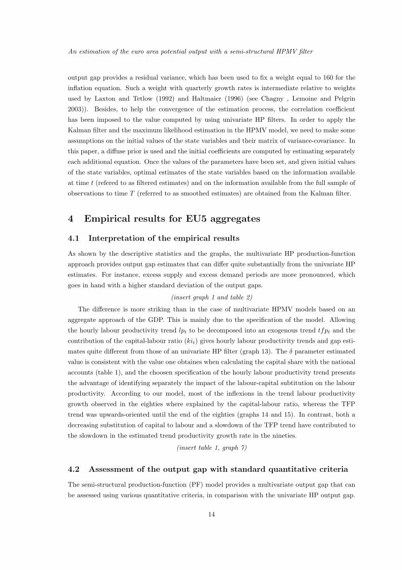
output gap provides a residual variance, which has been used to fix a weight equal to 160 for the

inflation equation. Such a weight with quarterly growth rates is intermediate relative to weights

used by Laxton and Tetlow (1992) and Haltmaier (1996) (see Chagny , Lemoine and Pelgrin

2003)). Besides, to help the convergence of the estimation process, the correlation coefficient

has been imposed to the value computed by using univariate HP filters. In order to apply the

Kalman filter and the maximum likelihood estimation in the HPMV model, we need to make some

assumptions on the initial values of the state variables and their matrix of variance-covariance. In

this paper, a diffuse prior is used and the initial coefficients are computed by estimating separately

each additional equation. Once the values of the parameters have been set, and given initial values

of the state variables, optimal estimates of the state variables based on the information available

at time t (refered to as filtered estimates) and on the information available from the full sample of

observations to time T (referred to as smoothed estimates) are obtained from the Kalman filter.

4 Empirical results for EU5 aggregates

4.1 Interpretation of the empirical results

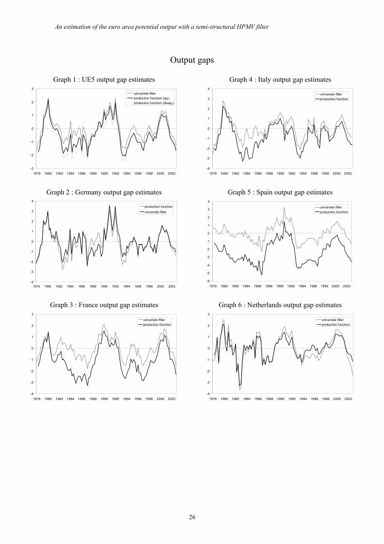
As shown by the descriptive statistics and the graphs, the multivariate HP production-function

approach provides output gap estimates that can differ quite substantially from the univariate HP

estimates. For instance, excess supply and excess demand periods are more pronounced, which

goes in hand with a higher standard deviation of the output gaps.

(insert graph 1 and table 2)

The difference is more striking than in the case of multivariate HPMV models based on an

aggregate approach of the GDP. This is mainly due to the specification of the model. Allowing

the hourly labour productivity trend lpt to be decomposed into an exogenous trend tfpt and the

contribution of the capital-labour ratio (kit) gives hourly labour productivity trends and gap esti-

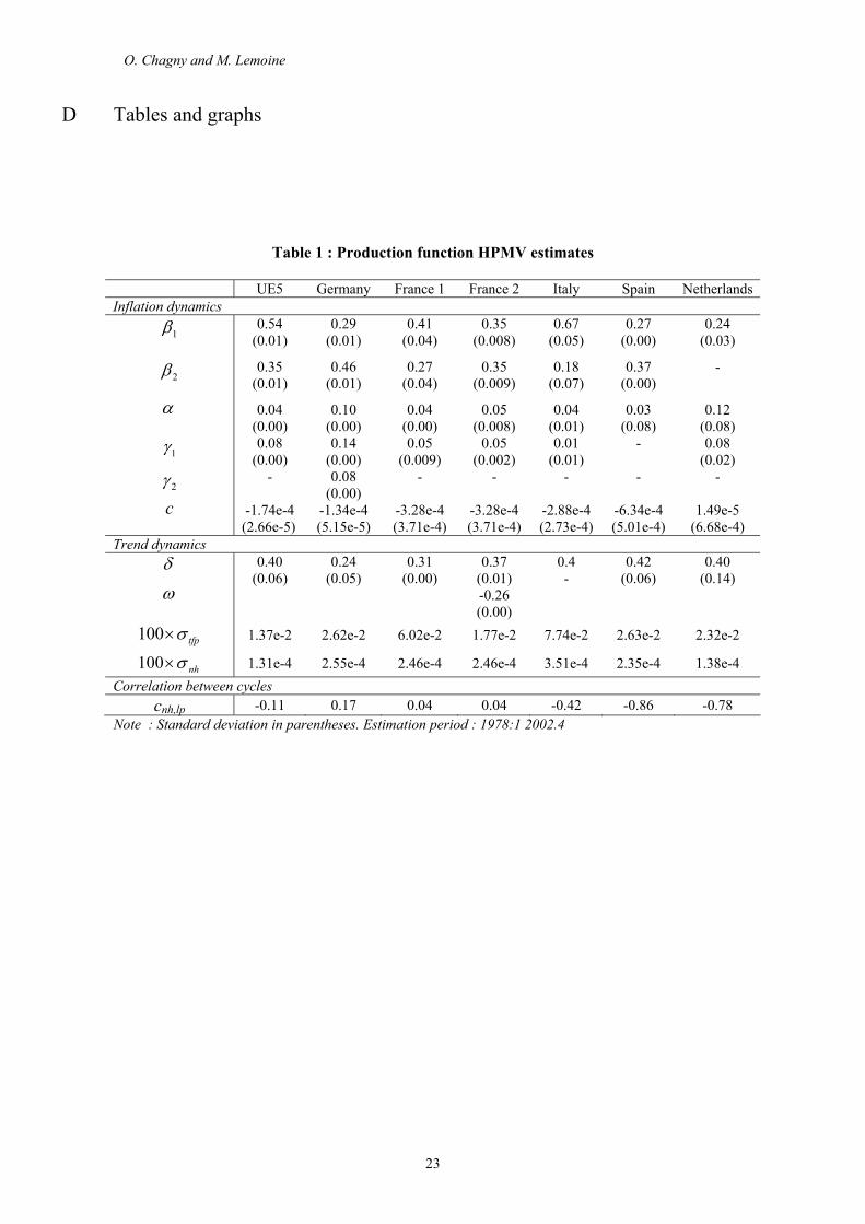
mates quite different from those of an univariate HP filter (graph 13). The δ parameter estimated

value is consistent with the value one obtaines when calculating the capital share with the national

accounts (table 1), and the choosen specification of the hourly labour productivity trend presents

the advantage of identifying separately the impact of the labour-capital subtitution on the labour

productivity. According to our model, most of the inflexions in the trend labour productivity

growth observed in the eighties where explained by the capital-labour ratio, whereas the TFP

trend was upwards-oriented until the end of the eighties (graphs 14 and 15). In contrast, both a

decreasing substitution of capital to labour and a slowdown of the TFP trend have contributed to

the slowdown in the estimated trend productivity growth rate in the nineties.

(insert table 1, graph 7)

4.2 Assessment of the output gap with standard quantitative criteria

The semi-structural production-function (PF) model provides a multivariate output gap that can

be assessed using various quantitative criteria, in comparison with the univariate HP output gap.

14


Two sets of criteria are considered, which concern the accuracy of the output gap estimates (table 4)

and their forecasting power regarding inflation (table 5) (see Appendices C and B for more details

on these criteria).

(insert tables 4 and 5)

Concerning the accuracy of the output gap estimates, the confidence bands are generally larger

with the production-function approach. The one-sided RMSE is equal to 0.82, as against 0.46 in

the case of the univariate HP filter. The two-sided RMSE is equal to 0.46, as against 0.25 in the

case of the univariate HP filter. However, one-sided and two-sided estimates of the PF output

gap also have larger standard deviation (1.60 and 1.18), than those of HP (0.99 and 0.90). We

therefore have to look at the Student statistics, which test whether the output gap estimate is

equal to zero (hypothesis H0). Student statistics of HP and PF estimates have very close values:

they stand above 1.8 for one-sided estimates and around 3 for two-sided estimates. Thus, H0

might be rejected with a risk equal to 90% with one-sided estimates and to 95% with two-sided

estimates. Concerning revisions between quasi-real-time and smooth estimates, multivariate PF

estimates have higer standard revisions (0.89) than univariate HP ones (0.76).

Although the accuracy of inflation prediction displays significant differences over the forecasting

horizons, the forecasting performance of the production-function approach can be considered as

broadly satisfactory. At a 10% level, the production-function model performs indeed better than a

naive random walk model over most of the horizons, and better than an AR(3) over long horizons6.

5 National production function models

Parameter estimates, descriptive statistics and graphs of the country-specific production-function

models output gaps are displayed in tables 1, 2 , 3 and graphs 2-6). Parameter estimates are

relatively heterogenous among countries, specifically for what concerns the inflation dynamics and

the labour market variables, a result which is consistent with the view that the euro area is still

characterized by a strong cross-country heterogeneity of the labour market institutions (see for

instance Fitoussi and Passet 2000). Despite this, the aggregation of the country-specific models

estimates provides potential output and output gap estimates which are very similar to those

obtained at the EU5 widel level (graph 1).

(Insert tables 1, 2, 3, graphs 1 to 6)

Even if they are functionnally more appropriated to capture economic structure differences

across countries, the production-function based approach exhibits agregation properties which are

in conclusion very similar to those observed with multivariate models based on a direct measure of

the GDP. The specification choosen for the model allows nevertheless to identify strong national

specificities with regard to the estimated hourly labour productivity trends (graphs 16 to 23). In

most of the countries considered here, the path of capital-labour substitution has been decreas-

ing since the mid-nineties, reflecting among others the effects of the wage moderation. But the

6However, one must keep in mind that the weight of the inflation equation has been arbitrarily fixed at a value

corresponding to a weight of 10 for year on year inflation.

15


slowdown is much less pronounced in Italy than in Spain for instance, which results in a smaller

contribution of the capital-labor ratio to the decrease of the labour productivity trend growth rate.

With regard to the capital-labour ratio, the Netherlands appear to be an outlier. The capital-labour

substitution has been practically stopped from the mid-eighties to the mid-nineties, and this is one

of the main factor explaining the slow growth rate of the total hourly labour productivity trend in

comparison to the other countries (1.4 percent per year in average over the period 1982-1993, to

compare with 2.4-2.6 percent in the other countries). In contrast, the capital-labour ratio has been

oriented upwards since 1998 in the Netherlands, which has contributed to moderate the slowdown

in the total labour productivity growth.

(Insert graphs 7 to 13)

Taking in account the capital-labour substitution reduces indeed substantially the cross-country

divergences. The average standard deviation of the total hourly labour productivity growth rate

trend (∆lp∗t ) is 0.86 over the period 1978:1 2002:4, but reduced to 0.66 for the the exogenous

technical progress trend (∆tfp∗t ). It also allows in principle to obtain a more consistent estimates

of the technical progress trend. But as displayed by the graphs 24 to 29, the 95 percent confidence

bands based on the filter uncertainty are large. For instance, estimated value for the exogenous

technical progress growth rate is -0.3% in 2002:4 in Italy, but 95% confidence upper and lower limit

are respectively 1.5% and -2.1%.

(Insert graphs 14 to 19)

A comparison of the two models estimated for France is proposed in graph 10 (see table 1 for

the parameter estimates). When the trend hourly labour productivity incorporates the impact of

the reduction of employer’s social contribution for low skilled labour lsk∗

t ,our estimates exhibit an

acceleration in the exogenous technical progress trend tfp∗t which is more pronounced since 1993.

Moreover, our model suggest that 300 000 job creations have been induced by this measure, an

estimation which is consistent with other sources (see DARES 2003 for a recent synthesis of the

employment policy in France).

6 Conclusion

Our results show that the multivariate HP production-function approach provides output gap

estimates that can differ quite substantially from the univariate HP estimates. As they are not

centered, they allow to take into account the desinflation which occured during the eighties in some

European countries. Concerning the accuracy of the output gap estimates, the confidence bands

are generally larger with the production-function approach, but the forecasting performance of the

production-function approach can be considered as broadly satisfactory. Concerning the compar-

ison of euro area wide and country-specific model, our results show that the aggregation of the

country-specific models estimates provides potential output and output gap estimates which are

very similar to those obtained at the EU5 wide level. The specification chosen for the model allows

nevertheless to identify national specificities. The model leaves room for economic determinants to

16


explain the potential output path, specifically for the hourly labour productivity trend. We illus-

trate this point in the case of France by identifying separately the effect of specific policy measures

in favour of low skilled labour on the labour productivity trend. Our results are consistent with

other sources. The approach presented in this paper can be subject to many further developments.

Use of translog production function would for instance permit to use a more complex functional

form of the production function than the Cobb-Douglas framework. We may also seek to improve

the measure of the capital-labour ratio, in order to remove the movements due solely to economic

fluctuations. Additional exogenous factors could also be integrated in the model, allowing, for

instance, to assess the impact of the underlying determinants of the capital-labour ratio.

References

BANQUE DE FRANCE, 2002, “Croissance potentielle et tensions inflationnistes”, Bulletin de

la Banque de France No 103.

BAXTER M. and KING R., 1995, “Measuring business cycles: approximate band-pass filters

for economic time series”, NBER Working Paper No 5022.

BENTOLILA S. and Gilles SAINT-PAUL, 2003, “Explaining movements in the Labor Share”,

Contributions to macroeconomics, Vol. 3 No 1.

BOURDIN J. and P. MARINI, 2003, “Une decennie de reformes fiscales en Europe : la France

a la traine”, Rapport du Senat No 343.

BROWN, R.S., D.W. CAVES, and L.R. CHRISTENSEN, 1979, “Modelling the structure of

cost and production for multiproduct firms”, Southern Economics Journal, 46, 2.

BUTLER L. ,1996, “A semi-structural method to estimate potential output: combining eco-

nomic theory with a time-series filter”, Bank of Canada Technical Report No. 76.

CAMBA-MENDEZ G. and D. RODRIGUEZ-PALENZUELA, 2003, “Assessment criteria for

output gap estimates”, Economic modelling, pp. 529-562.

CAYEN J.P and S. VAN NORDEN, 2002, “La fiabilite des estimations de l’ecart de production

au Canada”, Working paper Bank of Canada.

CHAGNY O., M. LEMOINE and F. PELGRIN, 2003, “An assessment of multivariate output

gap estimates in the Euro area”, Eurostat report, Project “Short term indicators for the Euro

zone”.

CHRISTENSEN, L.R., D.W. JORGENSEN, and L.J. LAU, 1973, “Transcendental logarithmic

production frontiers”, The Review of Economics and Statistics, 55, 1.

CLARK, T. E. and M. W. McCRACKEN, 2001, “Tests of forecast accuracy and encompassing

for nested models”, Journal of Econometrics, Vol 105, pp85-110.

DARES, 2003, “Les politiques de l’emploi et du marche du travail”, La Decouverte, collection

Reperes.

De MASI P., 1997, “IMF estimates of potential output: theory and practice.” Staff Studies for

the World Economic Outlook.

DENIS C., K. Mc MORROW and W. ROEGER, 2002, “Production function approach to

17


calculating potential growth and output gaps. Estimates for the EU Member States and the US”,

European Commission Economic Papers No 176.

DIEBOLD, F. X., and R. S. MARIANO, 1995, “Comparing predictive accuracy”, Journal

ofBusiness and Economic Statistics, Vol..13, No.3, pp. 253-63.

FITOUSSI J.P. and O. PASSET, 2000, “Reduction du chomage, les reussites en Europe”,

Rapport du Conseil d’Analyse Economique No 23.

GIORNO , P. RICHARDSON, D. ROESEVAERE and P. van den NOORD, 1995, ”Potential

output, output gaps and structural balance budgets”, OECD Economic Studies No 24.

GORDON R.J., 1997, “The Time Varying NAIRU and its implications for economic policy”,

Journal of Economic Perspectives, Vol. 11; N◦1, winter.

HAMILTON J.D., 1986, “A standard error for the estimated state vector of a state-space

model”, Journal of Econometrics, 52:129-57.

HALTMAIER J.,1996, “Inflation-adjusted potential output”, Board of Governors of the Federal

Reserve System International Finance Discussion Papers, No 561.

HARVEY A. C., 1989, Forecasting, Structural Time Series Models and the Kalman Filter,

Cambridge University Press.

HARVEY, D. I., S. J. LEYBOURNE and P. NEWBOLD, 1997, “Testing the equality of pre-

diction mean squared errors”, International Journal of Forecasting Vol. 13 No 2, pp281-291.

HODRICK, R. and PRESCOTT, E.C., 1980, “Post-war U.S. business cycles: an empirical

investigation”, Discussion Paper No 451, Carnegie-Mellon University, Pittsburgh, P.A.

KMENTA J., 1967, “On estimation of the CES production function”, International Economic

Review, Vol. 8 No 2.

KONGSAMUT P., S. REBELO and D. XIE, 1997, “Beyond Balanced Growth”, NBER Working

Paper No 6159.

LAXTON, D., and R. TETLOW, 1992, “A Simple Multivariate Filter for the Measurement of

Potential Output”, Technical Report No. 59. Bank of Canada.

Mc MORROW K. and W. ROGER, 2001, “Potential output: measurement methods, new

economy influences and scenarios for 2001-2010”, European Commission Economic Papers No

150.

OKUN, A., 1962, “Potential GDP: its measurement and significance”, American Statistical

Association, Proceedings of the Business and Economic Statistics Section: 98-103. Washington.

ORPHANIDES A. and S. VAN NORDEN, 1999, “The reliability of Output gap estimates in

real time”, Economic Discussion Series, Board of Governors of the Federal Reserve System.

ORPHANIDES A. and S. VAN NORDEN, 2003, “The reliability of inflation forecasts based

on output gap estimates in real time”, CIRANO working paper.

PESARAN M.H. and A. TIMMERMANN, 1992, “A simple nonparametric test of predictive

performance”, Journal of Business and Economic Statistics, Vol. 10, pp561-56.

PROIETTI T., A. MUSSO and T. WESTERMANN, 2002, “Estimating potential output and

the output gap for the euro area: a Model-Based Production Function Approach”, ECB Working

paper.

18


RICHARDSON P., L. BOONE, C. GIORNO, M. MEACCI, D. RAE and D. TURNER, 2000,

“The concept, policy use and measurement of structural unemployment: estimating a time varying

nairu across 21 OECD countries”, OECD Economic Department Working Paper No 250.

RUNSTLER G., 2002, “The information content of real-time output gap estimates. An appli-

cation to the euro area”, ECB Working Paper.

St AMANT P. and S. VAN NORDEN, 1997, “Measurement of the output-gap: a discussion of

recent research at the Bank of Canada”, Bank of Canada Technical Report No 79.

19


Appendices

A Description of the dataset

The database is quarterly. The sample covers the period extending from the first quarter of 1978

to the fourth quarter of 2002. Countries covered are Germany, France, Italy, the Netherlands

and Spain. As far as possible, data have been taken from the Eurostat national accounts. When

necessary, data have been back-calculated or are taken from the national sets of accounts. Specific

attention has been paid to using the same concepts and definitions for each country. EU5 data

are calculated as the aggregation of the five national data. German data have been retropolated

for the years preceding the reunification (first quarter of 1978 to fourth quarter of 1990) using the

data set published by the Statistisches Bundesamt, where national accounts aggregates for west

Germany have been harmonized with the ESA95 concepts and definitions.

Gross domestic product at constant prices: Eurostat and national sets of accounts,

billions of 1995 ECUs. Data are seasonally and working-day adjusted.

Private consumption and import of goods and services deflators: National sets of

accounts (billions of 1995 ECUs at constant prices, billions of current euros converted in ECUs

with the 1995 exchange rate for current prices). Data are seasonally and working-day adjusted.

Deflators for the EU5 data are calculated as the ratio of the aggregates in current prices to the

aggregates in constant prices.

Labour market data (employment, unemployment, working age population): Na-

tional accounts, European labour force survey (Eurostat), national labour force surveys and own

calculations. Employment: thousands of persons. ILO definition for unemployment. Labour mar-

ket data are fully consistent: labour force = working age population in employment + unemploy-

ment ; labour force ratio = ratio of the labour force to the working age population; unemployment

rate = ratio of the unemployment to the labour force. Annual data interpolated to quarterly data

for the working age population (15-64 years).

Hours worked: hours actually worked per person except for the Netherlands (hours paid

per job converted into hours per person) (Groningen University, OECD, national accounts, own

calculations). Annual data interpolated to quarterly data.

Capital stock in the business sector: capital stock in constant prices (converted into

billions of ECUs of 1995) of the total economy excluding government and housing taken from the

national accounts for Germany, and France. OECD time series converted into billions of 1995

ECUs for Italy, the Netherlands, and Spain. Annual data interpolated to quarterly data.

B Measures of forecasting performance

We test the forecasting performance of the different measures of the output gap by the root

mean squared error (RMSE) for multi-step ahead inflation forecasts.7 All models have hence been

7Other criteria can be used, as for instance the mean absolute error. Results are robust to alternative measures

of forecasting performances.

20


recursively estimated from 1978Q1 to i=1996Q4...2002Q3, and out-of-samples forecasts from 1 to

10 quarters ahead have been computed over the period 1997Q1-2002Q4.

The RMSE for any forecast is the square root of the arithmetic average of the squared differ-

ences between the actual inflation rate and the predicted inflation rate over one-period for which

simulated forecasts are constructed. As it is common in the literature, we use two reference models:

a “naive” random walk and an AR(3) process.8 We compare the accuracy of the inflation forecasts

to our reference model by comparing the RMSE of the two sets of forecasts. Specifically, we form

the ratio (Theil statistics) of the RMSE for each model of output gap to the RMSE for the naive

model (or AR(3) model). A ratio greater than one thus indicates that output gap model’s forecast

is less accurate than the “naive” or AR(3) models.9

We use the test of predictive performance proposed by Diebold and Mariano (1995) to introduce

a formal statistical procedure. The procedure is designed to test the null hypothesis of equality of

expected forecast performance by considering the mean of the difference of the RMSE of a pair of

two competing models. Let us suppose that a pair of h-step ahead forecast have produced forecasts

errors (e1t, e2t), t = 1, 2, ..., T and the RMSE is the specified function of the forecast error. Then

the null hypothesis of the Diebold-Mariano test is:

E[RMSE(e1t) − RMSE(e2t)] = 0.

Defining dt = RMSE(e1t)−RMSE(e2t), t = 1, 2, ..., T , the Diebold-Mariano test statistic is then:

SDM =[V (d)

]−1/2

dd→ N(0, 1)

where V (d) ≈ T−1

[γ0 + 2

h−1∑k=1

(1 −

kh

)γk

]and γk = T−1

T∑t=k+1

(dt − d)(dt−k − d).10

However, as is noted by Diebold and Mariano (1995), simulation evidence suggests that their

test could be seriously over-sized in the case of two-steps ahead prediction and the problem become

more acute as the forecasting horizon increases. In this respect, Harvey, Leybourne and Newbold

(1997) proposed employing an approximately unbiased estimator of the variance of d, which leads

to a modified Diebold-Mariano test statistic:

S∗ =

[T + 1 − 2h + T−1h(h − 1)

T

]SDM .

Harvey et al. (1997), Clark and McCracken (2001) show that this modified test statistic performs

better than the DM test statistic even if it still performs poorly in finite samples (Clark and

McCracken, 2001). They also show that the power of the test is improved, when p-values are

computed with a Student distribution.

8In the case of SVAR models, we use an AR(3) in first differences in order to be consistent.9It is to to be noted that the significance of the relative mean squared error (RRMSE) is not directly tested.

Indeed, the one-sided test H0 :RRMSE=1 againt H0 :RRMSE < 1 can be used and the corresponding p-values

measure type-I error associated with the test.10Diebold and Mariano (1995) initially proposed an estimate of V (d) that was not always positive semi-definite.

In this paper, a consistent estimate of the standard deviation is constructed from a weighted sum of the available

sample autocovariances of the loss differential vector - the difference between the squared forecast error of the models

and that of the reference model. Chosen weights insure that the matrix V (d) is positive semi-definite (Newey and

West, 1987).

21


C Measures of uncertainty and consistency

The statistical reliability of the output gap is also assessed by distinguishing the filter uncertainty

and the parameter uncertainty . As it is common in the literature, we use the decomposition of

Hamilton (1986):

E(Cy

t,t(θ) − Ct

)2

= E(Cy

t,t(θ) − Ct(θ))2

+ Σt,t(θ)

where Cyt,t(θ) is the estimate of the output gap given (yt)1..T and the parameter estimate θ. The

left-hand side term is the parameter uncertainty, directly obtained from the Kalman filter at each

date t. The second term of the right-hand side expression is the filter uncertainty (ΣPt,t). It needs

to be computed by a Monte-Carlo simulation procedure as follows:

• Draw K parameters (θk)k=1..K from a normal distribution N(θ, σ2

θ);

• Compute the corresponding K cycles Ct(θk) with the Kalman filter;

• For each date t, the parameter uncertainty is defined by a mean square error criterion:

ΣPt,t =

1

K

K∑

k=1

[Ct(θk) − Ct(θ)

]2

.

In addition, we also compare the one-sided/filtered estimates and the two-sided/smoothed

estimates by computing the parameter and filter uncertainty of smoothed estimates(ΣT,t,Σ

PT,t

).

Both sources of uncertainty are also characterised. Orphanides and Van Norden (1999), Cayen and

Van Norden (2002) proposed a battery of descriptive statistics but no formal testing in order to

evaluate the estimates of the output gap using real time data, final data or quasi-real time data.

Specifically, Orphanides and Van Norden (2003) find large discrepancies between the sequentially

estimated measures of the output gap when compared with final estimates. The disparities are

explained by the unreliability of the models in estimating end of sample values and to a lower

extent by data revisions. However, Orphanides and Van Norden (2003) mainly compare univariate

methods. Camba-Mendez and Rodriguez-Palenzuela (2003) assess the consistency of output gap

estimates by implementing the Pesaran and Timmermann (1992) test of directional change and a

Fisher test to compare the variances of recursively estimated output gap sequence and the finally

estimated sequence. Camba-Mendez and Rodriguez-Palenzuela (2003) show that the concern of

reliability of estimates may be to some extent overdone in the Euro-area. However, Van Norden

(2003) casts some doubts on their conclusion.

22


D Tables and graphs

Table 1 : Production function HPMV estimates

UE5 Germany France 1 France 2 Italy Spain Netherlands

Inflation dynamics

1β

0.54

(0.01)

0.29

(0.01)

0.41

(0.04)

0.35

(0.008)

0.67

(0.05)

0.27

(0.00)

0.24

(0.03)

2β

0.35

(0.01)

0.46

(0.01)

0.27

(0.04)

0.35

(0.009)

0.18

(0.07)

0.37

(0.00)

-

α 0.04

(0.00)

0.10

(0.00)

0.04

(0.00)

0.05

(0.008)

0.04

(0.01)

0.03

(0.08)

0.12

(0.08)

1γ 0.08

(0.00)

0.14

(0.00)

0.05

(0.009)

0.05

(0.002)

0.01

(0.01)

- 0.08

(0.02)

2γ - 0.08

(0.00)

- - - - -

c -1.74e-4

(2.66e-5) -1.34e-4

(5.15e-5)

-3.28e-4

(3.71e-4)

-3.28e-4

(3.71e-4)

-2.88e-4

(2.73e-4)

-6.34e-4

(5.01e-4)

1.49e-5

(6.68e-4)

Trend dynamics δ 0.40

(0.06)

0.24

(0.05)

0.31

(0.00)

0.37

(0.01)

0.4

-

0.42

(0.06)

0.40

(0.14) ω -0.26

(0.00)

100 σ× tfp 1.37e-2 2.62e-2 6.02e-2 1.77e-2 7.74e-2 2.63e-2 2.32e-2

100 σ× nh 1.31e-4 2.55e-4 2.46e-4 2.46e-4 3.51e-4 2.35e-4 1.38e-4

Correlation between cycles

cnh,lp -0.11 0.17 0.04 0.04 -0.42 -0.86 -0.78

Note : Standard deviation in parentheses. Estimation period : 1978:1 2002.4

23


Table 2: Descriptive Statistics of UE5 output gaps and trendsa

UE5 aggregate

(production

function)

UE5 aggregate

(univariate HP

filter)

UE5 national

approach

(production

function)

(1) Mean -0.43 0.02 -0.67

(2) Standard deviation 1.01 0.89 1.03

(3) Minimum -2.14 -1.71 -2.46

(4) Maximum 2.14 2.34 1.96

(5) Actual potential

output growth rateb

2.05 1.99 2.07

(6) Standard deviation

of potential output

growth rate

0.53 0.59 0.54

Note : statistics are reported for the period 1978:2 2002:4.

a : data are in percentage points. Growth rates have been annualised in the raw (5) and (6).

b : calculated as the growth rate of the trend output at the fourth quarter of the year 2002.

Table 3: Descriptive Statistics of national output gaps and trendsa

Germ.

(prod.

func.)

Germ.

(univ.

HP)

France

1

(prod.

func.)

France

2

(prod.

func.)

France

(univ.

HP)

Italy

(prod.

func.)

Italy

(univ.

HP)

Spain

(prod.

func.)

Spain

(univ.

HP)

Neth.

(prod.

func.)

Neth.

(univ.

HP)

(1) Mean -0.13 0.02 -1.03 -0.80 0.01 -0.75 0.03 -2.39 -0.01 0.00 0.01

(2) Standard

deviation 1.20 1.19 1.25 1.24 0.90 1.22 1.00 1.40 1.04 0.94 1.19

(3) Minimum -2.75 -2.43 -3.30 -3.06 -1.80 -3.27 -2.09 -5.25 -2.32 -3.32 -3.65

(4) Maximum 3.08 3.57 1.55 1.90 2.15 2.23 2.78 1.46 3.27 2.12 2.52

(5) Actual

pot. output

growth r.b 1.51 1.35 2.81 2.74 2.62 1.71 1.72 3.31 3.23 1.16 2.08

(6) St. dev. of

pot. output

growth r. 0.92 0.81 0.46 0.49 0.61 0.49 0.49 0.97 1.13 1.01 0.87

Note : statistics are reported for the period 1978:2 2002:4.

a : data are in percentage points. Growth rates have been annualised in the raw (5).

b : calculated as the growth rate of the trend output at the fourth quarter of the year 2002.

24


Table 4 : UE5 output gaps accuracy (1978:1 2002:4) and revisions statistics (1997:1 2002:4)

UE5 aggregate

(function

production )

UE5 aggregate

(univariate HP

filter)

Smoothed estimation

Total uncertainty 0.460 0.253

Filtered

uncertainty

0.449 0.253

Parametric

uncertainty

0.091 -

Filtered estimation

Total uncertainty 0.820 0.460

Filtered

uncertainty

0.809 0.460

Parametric

uncertainty

0.116 -

Output gap standard deviation

Smoothed1 1.181

(2.56)

0.897

(3.54)

Filtered1 1.596

(1.95)

0.994

(2.16)

Standard deviation of revisions

Quasi-real time 0.890 0.764

Note: t-student in parentheses.

Table 5 : Out-of-sample inflation forecasting performances (UE5 aggregate estimates)

Horizon AR(3) Random walk

Naïve

model

RMSE RRMSE DM P-value RMSE RRMSE DM P-value

1 0.219 1.000 0.000 1.000 0.260 1.000 .000 1.000

2 0.221 1.000 0.000 1.000 0.280 1.000 .000 1.000

3 0.225 1.000 0.000 1.000 0.244 1.000 .000 1.000

4 0.217 1.000 0.000 1.000 0.327 1.000 .000 1.000

5 0.220 1.000 0.000 1.000 0.337 1.000 .000 1.000

10 0.238 1.000 0.000 1.000 0.295 1.000 .000 1.000

UE5 aggregate model

1 0.178 0.813 -1.208 0.247 0.178 0.686 -1.622 0.127

2 0.171 0.771 -1.615 0.129 0.171 0.609 -2.647 0.019

3 0.173 0.770 -2.019 0.063 0.173 0.712 -1.850 0.085

4 0.164 0.756 -1.565 0.140 0.164 0.503 -3.098 0.008

5 0.159 0.726 -2.328 0.035 0.159 0.472 -3.561 0.003

10 0.159 0.670 -2.100 0.054 0.159 0.541 -2.758 0.015

N.B. The table compares the one to ten steps ahead inflation forecasts(out of sample) of the production function estimates to

the one to ten steps ahead inflation forecasts of two naive models (an AR(3) model and a random walk).

The RMSE (root mean squared error) is the square root of the mean prediction errors. The RRMSE is the relative root mean

squared error of the models against that of the naive models. The D-M statistics is the modified Diebold-Mariano (Diebold

and Mariano 1995, Harvey Leybourne and Newbold 1997) test statistics. P value is the marginal probability of the Diebold-

Mariano test of the null hypothesis of equal predictive accuracy of the alternative models and of the naive model.

25


Output gaps

Graph 1 : UE5 output gap estimates

-3

-2

-1

0

1

2

3

1978 1980 1982 1984 1986 1988 1990 1992 1994 1996 1998 2000 2002

univariate filter

production function (ag.)

production function (disag.)

Graph 2 : Germany output gap estimates

-4

-3

-2

-1

0

1

2

3

4

1978 1980 1982 1984 1986 1988 1990 1992 1994 1996 1998 2000 2002

production function

univariate filter

Graph 3 : France output gap estimates

-4

-3

-2

-1

0

1

2

3

1978 1980 1982 1984 1986 1988 1990 1992 1994 1996 1998 2000 2002

univariate filter

production function

Graph 4 : Italy output gap estimates

-4

-3

-2

-1

0

1

2

3

4

1978 1980 1982 1984 1986 1988 1990 1992 1994 1996 1998 2000 2002

univariate filter

production function

Graph 5 : Spain output gap estimates

-6

-5

-4

-3

-2

-1

0

1

2

3

4

1978 1980 1982 1984 1986 1988 1990 1992 1994 1996 1998 2000 2002

univariate filter

production function

Graph 6 : Netherlands output gap estimates

-4

-3

-2

-1

0

1

2

3

1978 1980 1982 1984 1986 1988 1990 1992 1994 1996 1998 2000 2002

univariate filter

production function

26


Labour productivity gaps and trends

Graph 7 : UE5 trend hourly labour productivity

0

0.5

1

1.5

2

2.5

3

1978 1980 1982 1984 1986 1988 1990 1992 1994 1996 1998 2000 2002

Univariate trend

Multivariate trend

TFP trend

In %, annual growth rates

Graph 8 : Germany trend hourly labour productivity

0

0.5

1

1.5

2

2.5

3

3.5

4

1978 1980 1982 1984 1986 1988 1990 1992 1994 1996 1998 2000 2002

Univariate trend

Multivariate trend

TFP trend


Graph 9 : France (1) trend hourly labour productivity

0

0.5

1

1.5

2

2.5

3

3.5

4

1978 1980 1982 1984 1986 1988 1990 1992 1994 1996 1998 2000 2002

Univariate trend

Multivariate trend

TFP trend


Graph 10 : France (1) and (2), comparison of trend

hourly labour productivity

0

0.5

1

1.5

2

2.5

3

3.5

4

1978 1980 1982 1984 1986 1988 1990 1992 1994 1996 1998 2000 2002

Multivariate trend

Multivariate trend (model with lsk)

TFP trend

TFP trend (model with lsk)


Graph 11 : Italy trend hourly labour productivity

-0.5

0

0.5

1

1.5

2

2.5

3

1978 1980 1982 1984 1986 1988 1990 1992 1994 1996 1998 2000 2002

Univariate trend

Multivariate trend

TFP trend


Graph 12 : Spain trend hourly labour productivity

-2

-1

0

1

2

3

4

5

6

1978 1980 1982 1984 1986 1988 1990 1992 1994 1996 1998 2000 2002

Univariate trend

Multivariate trend

TFP trend


Graph 13 : Netherlands trend hourly labour

productivity

-2

-1

0

1

2

3

4

1978 1980 1982 1984 1986 1988 1990 1992 1994 1996 1998 2000 2002

Univariate trend

Multivariate trend

TFP trend


27


Confidence bands of the endogenous productivity trends growth rates

Graph 14 : Confidence band UE5

-0.2

0

0.2

0.4

0.6

0.8

1

1.2

1.4

1.6

1.8

2

1978:02:00 1982:02:00 1986:02:00 1990:02:00 1994:02:00 1998:02:00 2002:02:00

UE5

UEmin

UEmax

Graph 15 : Confidence band Germany

-0.5

0

0.5

1

1.5

2

2.5

3

3.5

1978:02:00 1982:02:00 1986:02:00 1990:02:00 1994:02:00 1998:02:00 2002:02:00

GE

GEmin

GEmax

Graph 16 : Confidence band France (1)

-0.5

0

0.5

1

1.5

2

2.5

3

1978:02:00 1982:02:00 1986:02:00 1990:02:00 1994:02:00 1998:02:00 2002:02:00

FR

FRmin

FRmax

Graph 17 : Confidence band Italy

-3

-2

-1

0

1

2

3

4

1978:02:00 1982:02:00 1986:02:00 1990:02:00 1994:02:00 1998:02:00 2002:02:00

IT

ITmin

FRmax

Graph 18 : Confidence band Spain

-2

-1.5

-1

-0.5

0

0.5

1

1.5

2

2.5

1978:02:00 1982:02:00 1986:02:00 1990:02:00 1994:02:00 1998:02:00 2002:02:00

ES

ESmin

ESmax

Graph 19 : Confidence band Netherlands

-6

-5

-4

-3

-2

-1

0

1

2

3

4

5

1978:02:00 1982:02:00 1986:02:00 1990:02:00 1994:02:00 1998:02:00 2002:02:00

NL

NLmin

NLmax

20

An estimation of the Euro Area potential output with a ... gaps for the euro area combining...

Documents

Transcript of An estimation of the Euro Area potential output with a ... gaps for the euro area combining...