An Equilibrium Model of Entrusted Loans∗

Ying Liu§

Job Market Paper

November 21, 2017

Click here for the latest version

Abstract

Entrusted loans are inter-corporate loans and a major component of shadow bank-

ing in China. In a model with entrepreneurial moral hazard and bank moral hazard,

entrusted loans arise endogenously when the banking sector is competitive. Entrusted

loans involve a lending chain in which high-capitalized firms channel bank loans into

medium-capitalized firms. High-capitalized firms obtain cheap bank loans and over-

borrow to form shadow banks with the extra capital. Medium-capitalized firms si-

multaneously borrow from both banks and shadow banks, while low and semi-highly

capitalized firms borrow only from banks. As a result of lower bank monitoring, en-

trusted loans improve entrepreneurs’ welfare. However, entrusted loans destroy firms’

value because firms earn reduced expected profits. Default risk is increased and real

efficiency reduced.

Keywords: Shadow Banking, Entrusted Loans, Moral Hazard, Corporate Structure

JEL: G21, G28, G32, G38

∗I would like to thank my supervisor Norman Schurhoff for his helpful comments and advice. I amalso grateful for comments received from Theodosios Dimopoulos, John Duca, Artem Neklyudov, StevenOngena, Jean-Charles Rochet, and from seminar and conference participants at IFABS Ningbo conference,UNIL brown bag seminar and HEC Paris Finance PhD workshop.

§University of Lausanne and Swiss Finance Institute; E-mail: ying.liu@unil.ch; Website:https://yingliu-finance.com.

1 Introduction

Since the 2007-2008 global financial crisis, shadow banking in China has undergone rapid

growth. The size of this sector accounted for 39 percent of China’s GDP at the end of

2012, and in 2016, it already amounted to about $8.5 trillion, equivalent to 80 percent of

China’s GDP, as reported by Moody’s. A dominant form of China’s shadow banking is

entrusted loans.1 Entrusted loans are inter-corporate loans in which a financial institution

acts as a trustee, and the lender and borrower directly negotiate the terms of the loan. The

trustee merely acts as a middleman to facilitate the transaction for legal reasons. Classical

banking theories posit that banks differ from other credit suppliers in that banks screen or

monitor borrowers.2 Entrusted loans are associated with direct inter-corporate lending, so

the borrowing firms are subject to little or no monitoring by the lending firms. Despite being

suboptimal to bank loans regarding monitoring, entrusted loans are becoming prevalent in

China.3 This phenomenon raises a puzzle. Why do firms rely on other firms to obtain

financing, rather than specialized financial intermediaries such as banks?

In this paper, I provide an economic rationale for why entrusted loans endogenously

emerge as a form of shadow banking. I show that when the banking sector is perfectly

competitive, the interplay of entrepreneurial hazard and bank moral hazard results in a

lending chain in which firms with access to cheap bank loans recycle the loans by granting

entrusted loans to other firms. In addition to characterizing the feature of firms engaged in

entrusted loans, my model shows that entrusted loans improve entrepreneurs’ welfare but

destroy firms’ value and reduce real efficiency.

1Shadow banking has different forms in China, such as, entrusted loans, wealth management productsand trust loans (Elliott, Kroeber, and Qiao (2015), Elliott and Qiao (2015)).

2See, for example, Diamond (1984).3Entrusted loans were the largest component of China’s shadow banking sector until 2014. Since 2015,

entrusted loans are the second largest component and wealth management products become the largest one.As documented by Allen, Qian, Tu, and Yu (2017), entrusted loans constituted 32% of shadow bankingin terms of RMB amount at the end of 2012. Outstanding amount of entrusted loans has jumped to 13.2trillion RMB ($1.92 trillion) in 2016.

1

I develop a model based on Besanko and Kanatas (1993) with firms differing in their

capitalization, as in Holmstrom and Tirole (1997). Each firm invests own capital and raises

the remaining part through bank loans or entrusted loans to undertake risky investment

project. Limited liability induces entrepreneur to choose effort that influences the success

probability of project. Banks grant loans and monitor firms so that entrepreneurs exert more

effort than they would without bank monitoring. The new element I introduce is that firms

may form shadow banks and issue entrusted loans to other firms. The difference between

banking and shadow banking, apart from the source of financing, is that shadow banks

exert no monitoring efforts compared to banks. Shadow banking is, thus, a different lending

technology.

When the banking sector is perfectly competitive, there exists an equilibrium in which

high-capitalized firms over-borrow from banks and form shadow banks with their extra cap-

ital. The reason for which entrusted loans arise in the presence of a competitive banking

sector is the following. In a competitive environment, the bank gets zero surplus, and bor-

rower surplus is maximized. Given that bank monitoring is costly and unobservable, banks

are subject to the moral hazard problem when choosing monitoring intensity. Monitoring

costs must be incorporated into loan interest rates to incentivize banks to provide monitor-

ing. As firm’s capitalization reduces, bank loan demand increases, the interest rate on bank

loan also increases so that bank has a greater incentive to monitor the firm to receive the

higher payoff if the project succeeds. The bank monitoring cost is an increasing, convex

function of monitoring intensity, so bank interest rate has increasing return to scale. There-

fore, high-capitalized firms have the advantage of obtaining cheap bank loans and choose to

over-borrow. The increasing return to scale of bank interest rate creates opportunities for

high-capitalized firms to re-lend extra capital to other firms that incur expensive bank loans.

Medium-capitalized firms simultaneously borrow from both banks and shadow banks

while low and semi-highly capitalized firms only borrow from banks. Banks have an ad-

2

vantage in monitoring firms to alleviate entrepreneurial moral hazard, but banks cannot

commit to monitoring. The bank moral hazard induces banks to choose a monitoring level

to maximize bank profits, rather than maximizing entrepreneur utility. In this case, bank

monitoring forces entrepreneur to supply a level of effort that exceeds the one that would

be supplied without bank monitoring. Shadow banks do not monitor firms, so entrepreneurs

avoid effort costs by replacing bank loans with entrusted loans. A marginal increase of en-

trusted loans has two effects on entrepreneur’s expected utility: (1) the success probability

of investment project is reduced because of less bank monitoring; (2) entrepreneur obtains

higher payoff because of reduced effort. Low-capitalized firms are highly leveraged and en-

tail severe entrepreneurial moral hazard, a marginal increase of entrusted loans causes large

reduction of success probability which dominates the gain of entrepreneurial payoff, so these

firms are better off not taking entrusted loans. Semi-highly capitalized firms entail low en-

trepreneurial moral hazard, so the yield difference between bank loans and entrusted loans

is small, the increase of entrepreneur payoff by replacing bank loans with entrusted loans is

lower than the reduction of success probability, so entrepreneurs are better off not taking

entrusted loans. Therefore, the demand for entrusted loans displays a hump-shaped pattern

over firm capitalizations.

In the extension, I also consider the case that bank operates as a monopolist. En-

trusted loans do not exist in this situation. When the bank has monopoly power, the bank

loan contract is set to maximize bank’s profit, and the bank appropriates the surplus. Bank

internalizes the surplus when chooses monitoring intensity. The high surplus motivates the

bank to provide a high level of monitoring. The bank moral hazard problem is alleviated so

there is no role for entrusted loans.

To study the impact of shadow banking on social surplus and real efficiency, I examine

a benchmark model in which entrusted loans are prohibited. In the benchmark, firms only

take bank loans which are just enough to finance their investment projects. In the presence

3

of entrusted loans, entrepreneurs’ welfare are improved, but firms’ value reduced. The reason

is that entrepreneurs maximize their utilities rather than firms’ profits. Bank monitoring

forces entrepreneurs to exert more effort than they would do without bank monitoring. By

participating in shadow banking, entrepreneurs can shirk and exert less effort. As a result,

the success probabilities of firm investment projects are reduced and thereby, real efficiency

declines.

This model can be extended in a number of directions. First, I include the restricted

industries which are prohibited from bank lending.4 The lenders of entrusted loans are

high-capitalized unrestricted firms; the borrowers become medium-capitalized unrestricted

firms and high-capitalized restricted firms. Interest rates of entrusted loans increase with

the proportion of restricted firms. Shadow banks are the only external financing source

for restricted firms, and thus, behave like a monopolist. Interest rates of entrusted loans

and the default risk of restricted firms are both higher than those of the unrestricted firms.

Second, I consider the case that lending firms can better monitor the borrowing firms than

banks if lending firms and borrowing firms are affiliated. For example, the lending firms

and borrowing firms belong to the same industry, or same business group. The main results

remain valid, and the model generates several new features: (i) credit rationing is alleviated,

(ii) the borrowing firms of entrusted loans earn higher expected profits and have lower default

risk than the benchmark. The reason is that substituting bank loans with shadow bank loans

results in the greater entrepreneurial effort and, thus, reduces default risk and improves firm’s

profit.

This paper also provides interpretations for some stylized facts. First, the result is

consistent with the findings from Allen, Qian, Tu, and Yu (2017) that the lenders of entrusted

4In China, such industries include the real estate, coal mining and shipbuilding industries (Elliott,Kroeber, and Qiao (2015)). Allen, Qian, Tu, and Yu (2017) find that close to half of non-affiliated entrustedloans flew into the real estate and construction industry. A Wall Street Journal article “A Partial Primerto China’s Biggest Shadow: Entrusted Loans(May 2, 2014)” reports that from 2004 to 2013, around 20% ofentrusted loans went to property sector.

4

loans are high-capitalized firms that can obtain cheap bank loans, and the borrowers are

medium-capitalized firms.5 The model shows that it is due to the competition and moral

hazard of banks. Second, Allen, Qian, Tu, and Yu (2017) and He, Lu, and Ongena (2016)

find that lenders of entrusted loans usually charge very high interest rates to non-affiliated

borrowing firms. The model assumes that the lenders do not monitor the borrowers, which

can be interpreted as the lenders and borrowers not being affiliated, so the lenders do not

have the knowledge or ability to monitor the borrowers. The lack of monitoring makes

the borrowers riskier, and thus the lenders have to charge high interest rates. Third, the

lenders simultaneously borrow from banks and re-lend to the borrowers in the model. This

“borrow in order to lend” activity is consistent with findings in Shin and Zhao (2013).

Forth, Allen, Qian, Tu, and Yu (2017) and He, Lu, and Ongena (2016) show that the

average abnormal return for the lenders of non-affiliated entrusted loans is negative after the

entrusted loans announcement. This paper shows that entrusted loans destroy firm value

and severely increase firm default risk because entrepreneurs do not behave diligently.

The rest of this paper is organized as follows. Section 2 relates this paper to previous

research. In Section 3, I describe the model and solve the benchmark. In Section 4, I

introduce the shadow banking sector and derive the equilibrium results. I discuss welfare

implications, and list the theoretical predictions in Section 5. In Section 6, I give three

possible extensions of the model. Section 7 concludes the paper.

2 Literature Review

To the best of my knowledge, this is the first theoretical model on entrusted loans. The

most related paper is that of Allen, Qian, Tu, and Yu (2017), in which the authors examine

entrusted loans with transaction-level data. They divide entrusted loans into affiliated loans

5Allen, Qian, Tu, and Yu (2017) find that lenders are well-capitalized firms with a median value of 4billion RMB. The borrowers are medium-size companies with a median value of 0.4 billion RMB.

5

and non-affiliated loans on the basis of firm relationships and show that the loan interest

rates incorporate both fundamental and informational risks. Another related paper is that

of He, Lu, and Ongena (2016), in which the authors assess the valuation effects of entrusted

loans by measuring the abnormal returns of stock prices after entrusted loan announcements.

Chen, Ren, and Zha (2017) focus on the impact of monetary policy on entrusted loans and

emphasize the different roles of state-owned banks and non-state-owned banks that work as

trustees of entrusted loans. Yu, Lee, and Fok (2015) find a significant and positive correlation

between high-interest entrusted loans and firms’ last period cash holdings.

This paper is also related to the theoretical studies on credit rationing and constrained

bank lending. On the one hand, some studies feature moral hazard. My paper belongs to

this strand. Similar papers, include those of Besanko and Kanatas (1993), Petersen and

Rajan (1995), Holmstrom and Tirole (1997), Repullo and Suarez (2000) and Allen, Carletti,

and Marquez (2011). On the other hand, studies focus on asymmetric information, such

as Stiglitz and Weiss (1981), Besanko and Thakor (1987a), Besanko and Thakor (1987b).

Different from the above papers, I include firm heterogeneity, and I also introduce the channel

of shadow banking. Therefore, I can model the endogenous emergence of shadow banking

and identify the characteristics of the firms engaged in this activity. Moreover, by focusing

on the moral hazard problem, I can study the impact of shadow banking on entrepreneurial

behavior and firm performance.

This paper also belongs to the branch of literature about China’s shadow banking.

Acharya, Qian, and Yang (2016) document another large component of shadow banking:

wealth management products (WMP). They show that when small and medium-sized banks

face strong competition from the ‘Big Four’ banks to acquire deposits, they significantly

increased the issuance of WMPs after the financial crisis. Dang, Wang, and Yao (2014)

explain the growth of shadow banking with “information sensitivity”, which is a measure

of tail risks. The rise of shadow banking is associated with the asymmetric perception of

6

information sensitivity from banks, shadow banks, and investors. Both Hachem and Song

(2017) and Chen, He, and Liu (2017) link shadow banking activities to fiscal policy. Hachem

and Song (2017) argue that the shadow banking system is related to the competition between

small and medium-sized banks and the ‘Big Four’ banks. Shadow banking is an intended

consequence of the liquidity rules. Chen, He, and Liu (2017) show that the growth of shadow

banking after 2012 is a hangover effect of the “4 trillion stimulus package”.

Other theoretical studies regard shadow banking as a problem of regulatory arbitrage.

Buchak, Matvos, Piskorski, and Seru (2017) find that the increased regulatory requirements

of banks account for 55% of shadow bank growth, and 35% of the growth comes from the

development of financial technology. Farhi and Tirole (2017) show that financial intermedi-

aries can migrate to shadow banking in response to regulatory requirements, and they also

study optimal regulation in the presence of the shadow banking sector. In my paper, shadow

banking is not caused by the regulatory burden of traditional banks, and the banks do not

have capital constraints in my model. Shadow banking is a market reaction to the high

competition of the banking sector. Moreover, entrusted loans are very similar to trade credit

as documented by Petersen and Rajan (1997) and Biais and Gollier (1997) in the sense that

both are inter-corporate financing. However, entrusted loans are not necessarily granted

between suppliers and customers, and there are no goods or service purchases involved in

entrusted loans.

3 Model

The model is built on Besanko and Kanatas (1993) with two innovations. First, entrusted

loans are introduced as an outside option, besides firm’s own investment project. Firms

have to decide whether to participate in entrusted loans. Second, firms have different capi-

talizations, as in Holmstrom and Tirole (1997). When taking risky investment projects, firms

7

invest all own capital and borrow the remaining from external financing. The introduction of

firm heterogeneity allows me to study the firm characteristics that are engaging in entrusted

loans.

The model contains two types of agents: firms and banks. All agents are assumed

to be risk neutral. There are two dates in the model: date 0 and 1. At date 0, each firm

tries to locate funding for a risky investment project. At date 1, returns from projects are

realized, firms are liquidated, and banks are paid off.

There is a continuum of firms. Each firm is characterized by the capital w ∈ [0, 1] it

holds. The set of firms is described by the probability density function g(w). All firms have

access to the same technology and invest the same risky project in the model. The project

requires investment 1 at date 0. If w < 1, the firm needs at least 1−w external financing to

undertake the project. At date 1, the project generates return either Q > 1 with probability

p (success) or 0 with probability 1− p (failure).

Firms are run by entrepreneurs. The probability that the project succeeds depends

on the effort the entrepreneur spends on the project. The cost of effort required to achieve

a success probability p is p2

2β, where β ∈ (0, 1

2] is the reciprocal of the marginal cost of effort.

For simplicity, p is also the total effort from the entrepreneur. If the entrepreneur wants

to increase the success probability of the project, she has to expend more effort, which will

reduce her utility. Moral hazard arises since the effort of the entrepreneur is unobservable

by the market.

When the firm is not able to be self-financed, it has to take a loan from the bank. The

banking sector is perfectly competitive, so profit of each bank is driven to zero. The function

of banks is twofold: providing financial credit to the firm; offering monitoring services to

improve entrepreneur performance. Banks have a comparative advantage at monitoring

firms, which alleviates the entrepreneur moral hazard problem. Monitoring carries a cost to

8

the bank, which is assumed to be

M(p− p0) =

(p− p0)2/2m, if p ≥ p0,

0, if p < p0.

p is the effort level desired by the bank, p0 denotes the entrepreneur effort were there no

bank monitoring and thus called entrepreneur non-monitoring effort, m ∈ (0, β) denotes

the reciprocal of the marginal cost of monitoring. The marginal monitoring cost of the

entrepreneur is smaller than the bank, so m < β. Bank monitoring raises the success

probability from p0 to p. In case the bank desired level p is lower than the entrepreneur

non-monitoring effort level p0, the bank does not monitor and the total effort p equals to

non-monitoring effort p0.

3.1 Entrepreneur effort and bank monitoring

The timing of the model is as follows. Banks set up loan contracts which specify the loan size

LB and corresponding repayment RB. Firms decide how much loans to take and invest in

the project. Then entrepreneurs choose effort level p0 and banks choose monitoring intensity

p− p0.

By back-ward induction, I first solve the optimal entrepreneur non-monitoring effort p0

and bank monitoring p−p0 for given bank loan size LB and repayment RB. The entrepreneur

chooses the effort to maximize her expected utility that is given by

p∗0 = arg maxp

p(Q−RB)

rf− p2

2β+ LB + w − 1 = min{β(Q−RB)

rf, 1},

where rf ≥ 1 is the gross risk-free interest rate. For ease of exposition, two assumptions are

made:

9

Assumption 1. βQrf≤ 1.

Assumption 2. βQ2

2r2f− 1 > 0.

Assumption 1 states that the first-best level of effort, equivalently the success probability is

not bigger than 1. Under this assumption, the non-monitoring effort is thus

p∗0 =β(Q−RB)

rf. (3.1)

Assumption 2 ensures that the maximized NPV of self-financed project is strictly positive,

otherwise the entrepreneur will not undertake the investment project. Assumption 1 and 2

together require that√

2βrf < Q ≤ rf

β.

Banks do not commit to monitor firms, and bank monitoring is also unobservable to

the market, so banks also incur moral hazard problem. The bank monitoring intensity is

chosen to maximize the expected profit of the bank, for given non-monitoring effort p∗0, that

is

maxp

pRB

rf− (p− p∗0)2

2m− LB.

The optimal bank monitoring is derived as

p∗ − p∗0 =mRB

rf. (3.2)

Equation (3.1) and (3.2) show that, both entrepreneur non-monitoring effort and bank mon-

itoring expenditure are proportional to their payoffs. The payoff to entrepreneur is the total

investment output deducted by repayment to the bank, so entrepreneurs of high-capitalized

firms are willing to spend more effort. Instead, bank monitoring intensity is higher for

medium-capitalized firms. Overall, the total optimal entrepreneur effort is given as

p∗ =βQ+ (m− β)RB

rf

10

3.2 Benchmark: bank lending with no shadow banking

For comparison, I start with the benchmark in which shadow banking is prohibited. In the

benchmark, banks are the only outside financing for all firms. Then the equilibrium bank

lending problem is equivalent to the question in Besanko and Kanatas (1993), except that

firms have different initial capital.

The equilibrium loan size LB and bank repayment RB are chosen to maximize the

entrepreneur’s expected utility, subject to three constraints: the zero-profit condition of the

bank, and two participation constraints of firms. The optimization problem of entrepreneur

is given as

maxLB ,RB

U =p∗(Q−RB)

rf− p∗2

2β+ LB + w − 1, (3.3)

subject to

LB =p∗RB

rf− (p∗ − p∗0)2

2m, (bank zero-profit condition)

LB + w ≥ 1, (firm participation constraint 1)

RB ≤ Q. (firm participation constraint 2)

The entrepreneur utility is composed by three parts: the expected discounted firm profit

p∗(Q−RB)rf

; the cost of entrepreneur effort −p∗2

2β; and retained capital LB + w − 1. The zero-

profit condition of bank comes from the fact that banking sector is perfectly competitive.

Participation constraint 1 states that total capital of each firm is enough to invest in the

project. If not, the firm will return the loan LB to the bank and give up the project.

Participation constraint 2 ensures that the payoff to the entrepreneur should be nonnegative

to incentive the expenditure of effort on the project.

The maximization problem is simplified by substituting the zero-profit condition into

the objective function and thereby eliminating LB. Moreover, the optimal entrepreneur non-

11

monitoring effort level (3.1) and bank monitoring (3.2) are impounded into the objective

function, which yields

maxRB

(m− β − m2

β)R2

B + βQ2

2r2f

− (1− w) (3.4)

subject to

(m− 2β)R2B + 2βQRB

2r2f

≥ 1− w, (3.5)

Q−RB ≥ 0. (3.6)

A third assumption is further required:

Assumption 3. m < β2

Assumption 3 ensures that the second order condition of the optimization problem is nega-

tive, so there exists an solution.

Solving the optimization problem of entrepreneur, yields the following results.

Lemma 1. In equilibrium, only firms with initial capital w ≥ wN ≡ 1 − β2Q2

2(2β−m)r2fborrow

from banks, other firms are not able to obtain bank loans.

Note that wN ≤ 0 when Q2 ≥ 2β(2 − m

β)r2f , that is, the profitability of investment

project is high enough such that all firms are financed. While wN > 0 when Q2 < 2β(2−m

β)r2f ,

then firms with initial capital w < wN are credit rationed by banks.

Lemma 2. In equilibrium, firms with capital w ∈ [wN , 1] take bank loan:

L∗B = 1− w ≡ LOBB . (3.7)

12

The required repayment to banks is

R∗B =βQ−

√β2Q2 − 2(2β −m)(1− w)r2

f

2β −m≡ ROB

B . (3.8)

Equation (3.7) states that entrepreneur only issues the minimum amount of debt that

is just enough to finance the project. Because of the marginal cost of debt, bank loan interest

rate, is higher than the marginal return of retained capital, which is risk-free rate. So there

is no need to hold capital. The interest rate of bank loan is computed as

ROBB

LOBB=βQ−

√β2Q2 − 2(2β −m)(1− w)r2

f

(2β −m)(1− w). (3.9)

Note that the interest rate decreases in firm capitalization w. The negative relationship

between bank loan interest rate and firm capitalization is due to two reasons. First, banks

price loans by incorporating risks of investment projects. When the firm is low capitalized

and invest less own capital in the risky project, the entrepreneur’s incentive to exert effort

declines, which results in a high probability of investment failure. Banks thus charge a

higher interest rate to compensate the risk of default. Secondly, banks also incorporate

the monitoring cost into the interest rate. Bank’s monitoring cost is a convex function of

expenditure; the expenditure is proportional to the exposure RB as shown by equation (3.2).

So the average monitoring cost increases in loan demand. Low capitalized firms take a large

amount of bank debt and thus incur higher monitoring cost. Overall, banks charge a higher

interest rate on low capitalized firms.

13

4 Shadow banking

In this section, shadow banking is introduced. Since shadow banking in this paper refers

to inter-corporate entrusted loans, there are still two types of agents in the model: firms

and banks. However, among the firms, some endogenously form shadow banks and provide

financing to other firms in the form of entrusted loans. To differentiate, the former firms are

merely called lenders and the latter ones borrowers of shadow banking.

The first question is to determine characteristics of firms participating in shadow

banking. Specifically, what kind of firms become lenders and borrowers of shadow banking.

Because all firms are in short of capital for investment project, the way lending firms can

finance borrowing firms is through over-borrowing from banks6. Therefore, firms’ decision of

whether participating in shadow banking as lenders is equivalent to whether over-borrowing

from banks or not.

Lemma 2 shows that firms optimally choose to borrow the minimum amount of bank

loan which is just enough to finance the risky project. That is because retained capital only

generates a return of risk-free rate, which is smaller than the borrowing rate. However, once

firms have access to another option which returns with a much higher rate, firms might be

willing to over-borrow and invest extra capital in the new option. That is the way I model

the emergence of shadow banking. Specifically, in the first step, shadow banking is simply

formalized by an outside investment option which generates an expected discounted rate of

return rs > 1. Firms can invest extra capital LB + w − 1 in the outside option. The value

of rs cannot be smaller than 1. Otherwise, firms are better off depositing the extra capital

and earn the discounted rate of return 1.

The lenders are firms that choose to over-borrow bank loans. The borrowers are

merely firms choosing to take shadow bank loans. After lenders are determined, and shadow

6Purely conducting lending activities without investing in own business is not allowed, otherwise, thefirm becomes a bank and has to follow all the requirements of bank and function like a bank.

14

banks are formed. All firms except lenders thereby have both banks and shadow banks as

outside financing sources. These firms will optimally choose from both sources.

The existence of shadow banking depends on the rate rs. The equilibrium value of

rs is determined by market clearing condition. That is, the total supply of entrusted loans

should be equal to total demand. Total supply is the aggregate extra capital from lenders,

and total demand is the aggregate demand from borrowers. The existence of shadow banking

is therefore equivalent to having a solution rs > 1 which solves the market clearing condition.

Although the emergence and lending of shadow banking are sequential, I take the two

procedures as simultaneous. In essence, the two procedures are both external fundraising

activities of firms. In a static model, I can study how banks and shadow banks interact in

providing loans to firms. The timeline is given in figure 1.

Figure 1: Time line of the model

0

Banks set the loan

contract.

Firms decide whether

to take bank loan, if

yes, firms also choose

loan volume LB .

Firms which take

loan LB > 1 − wform shadow

banking, and set

the entrusted

loan contract

Firms choose the

optimal bank loan

LB and shadow

bank loan LS .

Firms choose

the effort p0,

banks choose

the monitoring

intensity p − p0

1

Projects ma-

ture, claims are

settled

15

4.1 Endogenous emergence of shadow banking

Similar to the benchmark, except that return from extra capital is rs instead of 1. The bank

loan contract {LB, RB} is set so as to maximize the entrepreneur’s utility, which is given as

maxLB ,RB

U =p∗(Q−RB)

rf− p∗2

2β+ rs(LB + w − 1), (4.1)

subject to

LB =p∗RB

rf− (p∗ − p∗0)2

2m, (4.2)

LB + w ≥ 1, (4.3)

RB ≤ Q. (4.4)

Solving the optimization problem of entrepreneur, yields the following results.

Lemma 3. For given rs > 1, firms with capital w over-borrow from banks when

rs ≥ rs(w) = 1 +

m2

β+ β −m

2β −m

βQ√β2Q2 − 2(2β −m)(1− w)r2

f

− 1

. (4.5)

First, note that rs > 1, which is consistent with the assumption that rs > 1. Sec-

ondly, rs is firm specific, which is a decreasing function of w. It implies that firms that

hold high capitalization tend to over-borrow and thus become lenders of shadow bank-

ing. Inverse solution of (4.5) shows that lenders of shadow banking have initial capital

w ≥ 1 − β2Q2

2r2f

(rs−1)

[(2β−m)rs+

2m2

β−m

][(2β−m)rs+

m2

β−β]2 . This threshold value increases in rs. That is, high

expected rate of return of shadow banking drive up firm participations.

Proposition 1. For given rs > 1, firms with initial capital w ≥ 1−β2Q2

2r2f

(rs−1)

[(2β−m)rs+

2m2

β−m

][(2β−m)rs+

m2

β−β]2

over-borrow and form shadow banks with extra capital. Bank loan size and required repayment

16

are

L∗B =β2Q2

2r2f

(rs − 1)[(2β −m)rs + 2m2

β−m

][(2β −m)rs + m2

β− β

]2 ≡ LSB,

R∗B =βQ(rs − 1)

(2β −m)rs + m2

β− β≡ RS

B.

When entrepreneur chooses to over-borrow, the optimal loan size LSB does not de-

pend on firm capitalization w anymore. Instead, all lender firms take the same amount

of bank loan. The firm that is indifferent from over-borrowing or not has capital w =

1− β2Q2

2r2f

(rs−1)

[(2β−m)rs+

2m2

β−m

][(2β−m)rs+

m2

β−β]2 = 1− LSB. Note that the expected profit from outside option

rs(LB + w − 1) is a linear function of loan size LB, so firms are willing to take as much

bank loan as possible. However, on the other hand, taking more debt means entrepreneurs’

payoff from investment project will decline, and further discouraging entrepreneur behaving

diligently, worsening the expected profit of firm’s investment project. Therefore, the optimal

amount of bank loan is determined such that the return from shadow banking compensate

the reduction of entrepreneur utility.

Also, the required repayment RB and bank loan interest rate RBLB

are also independent

of w. Each lender firm has the same bank loan contract, each entrepreneur pays the same

amount of effort and bank expends the same monitoring. Entrepreneurs of lenders firms

obtain the same amount of utility, which equals to the utility of entrepreneur of the boundary

firm w = 1− LB could get.

4.2 Shadow bank lending

In the presence of shadow banks, all firms except lenders derived in section 4.1 optimally

choose loans from banks and shadow banks. The difference between banks and shadow banks

are twofolds: first, shadow banks do not provide monitoring service. Second, shadow banks

17

require a rate of return to be at least rs > 1, while the rate of return to bank is 1. Since

shadow banks compete with formal banks in providing capital to firms, the rate of return

from shadow banks is squeezed to rs. Similarly, the optimal bank loan contract {LB, RB}

and shadow bank loan contract {LS, RS} are selected to maximize entrepreneur’s utility,

which is given as

maxLB ,RB ,LS ,RS

U =p∗(Q−RB −RS)

rf− p∗2

2β+ LB + LS + w − 1 (4.6)

subject to

p∗RB

rf− (p∗ − p∗0)2

2m= LB, (4.7)

p∗RS

rf= rsLS, (4.8)

LB + LS + w − 1 ≥ 0, (4.9)

RB +RS ≤ Q. (4.10)

The inclusion of shadow banks bring several changes. First, entrepreneur’s optimal non-

monitoring effort becomes p∗0 = β(Q−RB−RS)rf

. The optimal bank monitoring effort p∗ − p∗0

keeps but the total entrepreneur effort becomes p∗ = βQ−βRS+(m−β)RBrf

. Second, if firms

decide to take both bank loan and shadow bank loan, that is, LB > 0 and LS > 0, total

loans should be enough to start the project, as indicated by (4.9). Meanwhile, total loan

repayments RB +RS should not exceed the investment return Q.

The rate of return from retained capital LB + LS + w − 1 is only 1 because there is

no second-tier shadow banking opportunity. In one case, suppose firm A over-borrows from

both bank and shadow bank, and A wants to lend out extra capital to firm B. Within the

capital A obtained, shadow bank requires a rate of return rs. When A lends to B, A expects

a rate of return which is higher than rs. However, in this case, B could borrow directly

18

from shadow bank, instead of A. So A loses the borrower market because of competition

from shadow bank. In another case, suppose firm A only borrows from banks and over-

borrows, then A lends to B. In this case, A must have initial capital w ≥ 1 − LSB, which

means A belongs to the lenders derived in section 4.1. Therefore, there is no second-tier

shadow banking opportunity and the rate of return from retained capital is 1. Solving the

entrepreneur’s optimization problem gives the equilibrium bank and shadow bank lending.

Proposition 2. Depending on the value of the expected rate of return of shadow banking rs,

optimal financing strategies of firms are given as

1. If rs ≥ 13

(1 + m

β+ 2√

1− mβ

+ m2

β2

)≡ rs, all firms with capital w ∈ [wN , 1 − LSB]

take only bank loans. Each firm borrows the minimum amount L∗B = 1− w, and bank

requires return

R∗B =βQ−

√β2Q2 − 2(2β −m)(1− w)r2

f

2β −m≡ ROB

B . (4.11)

Firms with capital w < wN can not get any financing.

2. If rs < rs, firms with capital w ∈ [w1, w2] borrow from both bank and shadow bank,

where

w1 = 1− βQ2(2−m

β)r2f

[1−

((rs−1)(m2+2mβ−2β2)+m(2−m

β)(m−√β2(1+2rs−3r2s)+2mβ(rs−1)+m2)

2(rs−1)(m2−mβ+β2)+2m2(2−mβ

)

)2],

w2 = 1− βQ2(2−m

β)r2f

[1−

((rs−1)(m2+2mβ−2β2)+m(2−m

β)(m+√β2(1+2rs−3r2s)+2mβ(rs−1)+m2)

2(rs−1)(m2−mβ+β2)+2m2(2−mβ

)

)2].

The equilibrium bank loan size L∗B ≡ LMB , bank repayment R∗B ≡ RMB , the equilibrium

shadow bank loan size L∗S ≡ LMS , shadow bank repayment R∗S ≡ RMS , are solutions to

19

the equation system

∂U∂LB

= ∂U∂LS

LB = βr2fRB

(Q−RS + (m

2β− 1)RB

)LS = β

rsr2fRS

(Q−RS + (m

β− 1)RB

)LB + LS = 1− w

LB ≥ 0, LS ≥ 0

(4.12)

Firm with capital w ∈ [wN , w1) or w ∈ (w2, 1−LSB] borrow only from banks. The bank

loan size is L∗B = 1− w and repayment to bank is R∗B = ROBB .

4.3 The existence of shadow banking

The existence of shadow banking is equivalent to the existence of a solution rs ∈ (1, rs) which

satisfies the market clearing condition: total supply of shadow bank capital equals to total

demand of shadow bank loan.

The supply of shadow bank comes from the extra capital of lenders derived in section

4.1, which is

TS =

∫ 1

1−LSB(LSB + w − 1)g(w)dw.

The demand of shadow bank loan is the total demand of the borrowers derived in section

4.2, that is,

TD =

∫ w2

w1

LSSg(w)dw.

The shadow banking exists if and only if there exists a solution rs ∈ (1, rs) that solves

TD = TS. Note that both total supply TS and total demand TD are functions of the

expected shadow banking rate rs, one can derive some properties of TS and TD with respect

20

to rs.

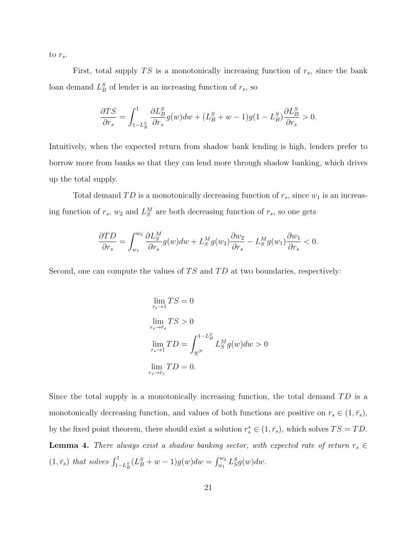
First, total supply TS is a monotonically increasing function of rs, since the bank

loan demand LSB of lender is an increasing function of rs, so

∂TS

∂rs=

∫ 1

1−LSB

∂LSB∂rs

g(w)dw + (LSB + w − 1)g(1− LSB)∂LSB∂rs

> 0.

Intuitively, when the expected return from shadow bank lending is high, lenders prefer to

borrow more from banks so that they can lend more through shadow banking, which drives

up the total supply.

Total demand TD is a monotonically decreasing function of rs, since w1 is an increas-

ing function of rs, w2 and LMS are both decreasing function of rs, so one gets

∂TD

∂rs=

∫ w2

w1

∂LMS∂rs

g(w)dw + LMS g(w2)∂w2

∂rs− LMS g(w1)

∂w1

∂rs< 0.

Second, one can compute the values of TS and TD at two boundaries, respectively:

limrs→1

TS = 0

limrs→rs

TS > 0

limrs→1

TD =

∫ 1−LSB

wNLMS g(w)dw > 0

limrs→rs

TD = 0.

Since the total supply is a monotonically increasing function, the total demand TD is a

monotonically decreasing function, and values of both functions are positive on rs ∈ (1, rs),

by the fixed point theorem, there should exist a solution r∗s ∈ (1, rs), which solves TS = TD.

Lemma 4. There always exist a shadow banking sector, with expected rate of return rs ∈

(1, rs) that solves∫ 1

1−LSB(LSB + w − 1)g(w)dw =

∫ w2

w1LSSg(w)dw.

21

I solve the model numerically by setting Q = 2.2, β = 0.5, m = 0.2, rf = 1.1

and assuming w follows uniform distribution on [0, 1]. The bank and shadow bank lending

are demonstrated in figure 8. Figure 8 shows that shadow bank loan demand LMS is a

concave function of firm capitalization w. That is due to the entrepreneur effort. When

firms simultaneously borrow from banks and shadow banks, banks provide monitoring which

guarantees a high level of success probability. Shadow banks free ride banks’ monitoring and

thus charge a lower interest rate because of no monitoring. So entrepreneurs are willing

to take shadow bank loans and thereby reduce the demand for bank loans. However, the

increase of shadow loan reduces the entrepreneur effort p because bank monitoring declines.

So entrepreneurs have to balance the tradeoff between increased payoff and reduced success

probability. For firms with low capitalization w ∈ [wN , w1), the reduction in p is much larger

than the increase in entrepreneur payoff, so entrepreneurs do not take shadow bank loans.

For firms with high capitalization w ∈ (w2, 1 − LSB], the increase in entrepreneur payoff is

smaller because these firms enjoy low bank interest rate, shadow loan rate is not competitive

as the bank loan rate, so entrepreneurs choose not to take shadow loans. For firms which

take both bank loans and shadow bank loans, the two loan demands are determined that

the marginal profit of bank loans and shadow bank loans be equal, as shown by (4.12).

I then compute and plot the interest rates of bank loan and shadow bank loan in figure

2. Figure (2a) shows the bank loan rates with and without shadow banking (benchmark),

as well as shadow bank loan rate. The green line represents the equilibrium bank lending

rate; the gray dotted line plots the bank lending rate in benchmark, the blue line plots the

shadow bank lending rate. Figure (2b) gives a clear illustration of how the bank lending rate

changes compared with the benchmark. Firms with the capital w ∈ [1 − LSB, 1] are lender

firms, firms with capital w ∈ [w1, w2] are borrower firms of shadow banking, other firms do

not participate in shadow banking.

First, note that both banks and shadow banks charge lower interest rate to high-

22

Figure 2: The comparison with and without shadow banking

(a) The lending rates(b) The change of bank lending rate from thebenchmark

capitalized firms and higher interest rate to medium-capitalized firms. They are mainly

driven by the default risk caused by moral hazard problem. Next, shadow bank interest

rates are smaller than bank interest rates. The difference comes from the bank monitoring

service. Banks monitor firms by paying a convex cost, so banks incorporate the cost into the

interest rate, which can be seen by deriving the interest rate from bank’s zero profit equation

(4.7):

RB

LB=rfp

(1 +

(p− p0)2

2mLB

)Shadow banks do not monitor firms, so shadow banks can charge a lower rate than bank

lending rate, as given by (4.8):

RS

LS=rfprs.

Since it is costly to monitoring medium-capitalized firms, the average monitoring cost in-

creases in firm capitalization w, so is the difference between bank and shadow bank lending

rates, as demonstrated by the green line and the blue line.

23

Moreover, in the presence of shadow banking, banks increase the lending rate to both

lender firms and borrower firms, which is illustrated in figure 2b. The adjustment is also

positively correlated with the involvement of shadow banking activities. That is because

participation of shadow banking discourages entrepreneur to perform diligently. The default

risk (1− p) of both lenders and borrowers thus increase, so banks incorporate the high risk

into the interest rates.

5 Welfare Analysis

To study the impact of shadow banking on social surplus and real efficiency, I compare

the equilibrium results with the benchmark where shadow banking is prohibited. Figure

9 illustrates the equilibrium results with and without entrusted loans (benchmark). Since

banks always obtain zero profit under the two situations, and proposition 2 shows that the

presence of shadow banking does not change the credit rationing, so I only focus on firms’

profits. Then, I study the impact of shadow banking on real efficiency by comparing the

success probabilities p of the investment project.

5.1 Firm’s profit

Entrusted loans affects two types of firms: firms with capitalization w ∈ (1 − LSB, 1] that

become the lenders of entrusted loans, and firms with capitalization w ∈ (w1, w2) that become

the borrowers. Note that the equilibrium bank loan contract {LB, RB} and entrusted loan

contract {LS, RS} are chosen to maximize the entrepreneur’s utility U , which is different

from firm’s profit π:

U = π − p2

2β. (5.1)

24

The entrepreneur’s utility U is lower than the firm’s profit π by p2

2β, that is the entrepreneur

effort cost. Using results from proposition 1 and 2, firm’s profit in the presence of shadow

banking is computed as

πF =

πOBF =(β−m)[β2Q2−r2f (2β−m)(1−w)]+(β2−mβ+m2

2)Q√β2Q2−2r2f (2β−m)(1−w)

(2β−m)2r2f, wN ≤ w < w1

πMF =[β(Q−RMS )+(m−β)RMB ](Q−RMB −RMS )

r2f, w1 ≤ w < w2

πOBF =(β−m)[β2Q2−r2f (2β−m)(1−w)]+(β2−mβ+m2

2)Q√β2Q2−2r2f (2β−m)(1−w)

(2β−m)2r2f, w2 ≤ w < 1− LSB

πSF =βQ2[2m4+2β4r3s−2m3β(rs+1)−mβ3rs(rs+1)+2β2m2rs(rs+2)]

2r2f(m2−mβrs+(2rs−1)β2)2 − rs(1− w), 1− LSB ≤ w ≤ 1

(5.2)

And firm’s profit in benchmark is

πOBF =(β −m)

[β2Q2 − r2

f (2β −m)(1− w)]

+ (β2 −mβ + m2

2)Q√β2Q2 − 2r2

f (2β −m)(1− w)

(2β −m)2r2f

.

(5.3)

Comparing lending firm’s profit πSF and borrowing firm’s profit πMF with the benchmark πOBF ,

respectively, yields

Lemma 5. In the presence of shadow banking, both the lending firms and borrowing firms

get lower expected profits:

πSF ≤ πOBF , πMF ≤ πOBF .

The declines in firms’ profits are due to the agency problem. Entrepreneur chooses

the debt level to maximize her utility, which equals to firm’s profit minus entrepreneur

effort cost, as shown by equation (5.1). Since bank also incurs moral hazard problem, bank

chooses the monitoring effort to maximize its profit, not entrepreneur utility. So the bank’s

monitoring forces entrepreneur to exert more effort than her desired level. More specifically,

banks force entrepreneurs to exert effort p, which is higher than entrepreneur’s desired level

25

p0. In the presence of entrusted loans, the lending firms replace bank loans with entrusted

loans and avoid the corresponding bank monitoring. The lending firms of entrusted loans

take excess loans which result in higher debt level, so the entrepreneurs also behave less

diligently because of moral hazard. Overall, by engaging in entrusted loans, entrepreneurs

obtain higher welfare, but firms earn lower expected profits as entrepreneurs exert less effort

than the benchmark.

I then compute the profits with the numerical results and plot the change of profit

100∗(πF −πOBF )/πOBF in Figure 3. The profits are reduced in the presence of entrusted loans.

The reduction is very significant for high-capitalized lending firms because these firms invest

a large amount in shadow banking. For the borrowers of entrusted loans, the reduction is

a concave function of firm capitalization, which is proportional to the demand of entrusted

loans of these firms. In other words, firms which participate more in shadow banking loose

more profit.

Figure 3: The change of firm profit with and without entrusted loans

26

5.2 Real efficiency

The probabilities of success or the total efforts from entrepreneur are demonstrated in figure

4. Figure 4a compares the total entrepreneur effort with the benchmark, figure 4b demon-

strates the change of entrepreneur effort compared with benchmark 100 ∗ (p − pOB)/pOB.

The total entrepreneur effort declines in the presence of entrusted loans. Similarly, the re-

duction is positively correlated with the involvement of shadow banking and more significant

for the lending firms. However, the reductions are due to different factors for the lending

firms and borrowing firms. Note that the total entrepreneur effort is the sum of entrepreneur

non-monitoring effort and bank monitoring effort. The reduction of lenders comes from the

decreased entrepreneur non-monitoring effort, while the reduction of borrowers is from the

decreased bank monitoring effort. The lenders increase the demand for bank loan since part

of the loan is invested in shadow banking, so the repayment to bank also increase, and the

projected return to entrepreneur is reduced. Entrepreneur thus reduces the non-monitoring

effort since it is proportional to the return: p0 = β(Q−RB)rf

. For the borrowing firms, the

demands of bank loans are reduced since part of bank loans are replaced by shadow bank

loans. Banks cut the monitoring effort because banks receive a reduced payoff. While shadow

banks do not provide monitoring service, the total entrepreneur effort thus is decreased.

27

Figure 4: The comparison with and without shadow banking

(a) The entrepreneur total effort

(b) The change of entrepreneur total effort

Taken together, the reduction of entrepreneur effort of both lending firms and bor-

rowing firms makes these firms riskier. Therefore, banks increase the lending rates of these

firms, as shown in figure 2b.

In conclusion, entrusted loans improve entrepreneurial welfare but reduce firms’ profit,

because entrepreneurs exert less effort than desired by the shareholders of firms. The drop

of entrepreneurial efforts also causes an increase in default risk.

5.3 Theoretical predictions

The theoretical model has shown that the existence of entrusted loan is related to the com-

petitive environment of the banking sector. Entrusted loans do not exist when the bank has

monopoly power (described in section 6.1). When the banking sector is perfectly competi-

tive, entrusted loans arise endogenously. Therefore, we should observe the banks are more

competitive along with soaring of entrusted loans.

28

Essentially, the cause of entrusted loan is the heterogeneity in the interest rates of bank

loan each firm has. Firms that can obtain cheap bank loan re-lend the loan to firms that

could only borrow with the high rate from the bank. So I postulate the first hypothesis:

Hypothesis 1. The bank lending rate is a decreasing function of firm capitalization, or an

increasing function of loan volume.

This hypothesis is based on Lemma 6. The theory shows that the high-capitalized

firm has lower monitoring cost, the entrepreneur also pays more effort on the investment

project. So the bank charges lower lending rate.

The next two hypotheses are related to the welfare analysis

Hypothesis 2. For firms with the same capitalization, the bank lending rates are higher to

firms that engage in shadow banking activities, than firms that do not.

Hypothesis 3. For firms with the same capitalization, the default risk(probability of success)

is higher to firms that engage in shadow banking activities, than firms that do not.

Hypothesis 2 could test whether the entrusted loans from the lending firms are natu-

rally the over-borrowed bank loans. Fixing the firm capitalization, the lenders of entrusted

loans have higher bank loan demands, according to hypothesis 1, the lending firms have to

pay a higher interest rate to the bank. Hypothesis 3 reflects the negative impact of the

entrusted loans to the involved firms. As an alternative investment project, entrusted loans

offer a higher payoff, the entrepreneurs thus reduce the efforts on firms’ investment projects,

resulting in a high default risk.

6 Extensions

Three extensions are considered in this section. In the first extension, I assume the banking

sector is non-competitive. In the second extension, I include restricted industries which are

prohibited from bank lending. In the third extension, I consider a special case that shadow

29

banks can better monitor borrowing firms than banks if the lending firms and borrowing

firms are affiliated.

6.1 Non-competitive banking sector

In this section, it is assumed that the banking sector is non-competitive. The bank has

monopoly power. I show that under this setting, entrusted loans do not exist. The reason

is that with monopoly power, the bank obtains positive surplus. A high surplus induces the

bank to provide a high level of monitoring, so bank moral hazard is alleviated. Note that

entrusted loans result from bank moral hazard when the bank moral hazard is not severe,

entrusted loans do not exist. To prove this, I first solve the optimal loan contract with a

non-competitive banking sector. The optimization problem is given as

maxLB ,RB ,p

p∗RB

rf− (p∗ − p∗0)2

2m− LB (6.1)

subject to

p∗(Q−RB)

rf− p∗2

2β+ rs(LB + w − 1) ≥ 0 (6.2)

LB + w − 1 ≥ 0 (6.3)

0 ≤ RB ≤ Q (6.4)

When the bank has monopoly power, the loan contract {LB, RB} are set to maximize the

bank’s profit. Three constraints have to be satisfied. 6.2 establishes that each firm gets

positive profit. 6.3 ensures that the firm gets enough financing for the investment project.

Last, the required repayment to the bank cannot exceed the total return from the project.

Note that the rate of return of retained capital LB + w − 1 is rs, the following result will

show that even if the firm has a profitable option (investing in shadow banking), the firm

30

chooses not to invest in this option.

Proposition 3. Under non-competitive banking sector, only firms with initial capital w ≥

wN can obtain bank financing, the firms with w < wN are not financed. The optimal loan

size, the bank repayment, and monitoring effort are given as

L∗B = 1− w, (6.5)

R∗B =βQ

2β −m≡ Rnc

B , (6.6)

p∗ =β

β −mp∗0 =

β2Q

(2β −m)rf≡ pnc. (6.7)

Each firm only borrows the amount of capital that is enough to undertake the investment

project, thus, shadow banking does not exist.

Each firm only borrows the minimum amount of capital 1−w from the bank. It implies

that shadow banking does not exist in a non-competitive banking environment. Further, I

compare the bank lending rates and total entrepreneur efforts (probability of success) under

a non-competitive banking environment to the benchmark. The comparisons are given as

follows.

Lemma 6. The lending rates are

RncB

LncB=

βQ

(2β −m)(1− w),

ROBB

LOBB=βQ−

√β2Q2 − 2(2β −m)(1− w)r2

f

(2β −m)(1− w),

and

RncB

LncB≥ ROB

B

LOBB. (6.8)

31

The entrepreneur total efforts are

pnc =βQ

rf

β

2β −m,

pOB =βQ

rf

β

2β −m+

β −m2β −m

√1−

2(2β −m)(1− w)r2f

β2Q2

,and

pOB ≥ pnc. (6.9)

Equations (6.8) and (6.9) show that under non-competitive banking environment,

the bank charges higher lending rate and the entrepreneur exerts less effort on the project,

compared to those in a competitive banking environment. The comparisons are demonstrated

in figure 5. The solid red line illustrates the non-competitive banking sector; the green line

illustrates the competitive banking sector.

Figure 5: The comparison between competitive and non-competitive banking environment

(a) The bank lending rates (b) The total entrepreneur efforts

The bank lending rate under a non-competitive banking environment is higher than

that in a competitive environment. The lending rate increases with firm capitalization w.

The bank has monopoly power and takes the most surplus from the lending. Equation (6.6)

32

shows that bank requires the same amount of repayment from each firm, and the repayment

is more than half of the investment return. Since the bank’s utility is negatively correlated

to the loan size LB, the bank only lends the minimum amount of capital to each firm. As a

result, high-capitalized firms borrow less but pay the same amount to the bank than other

firms. Thus the interest rates are higher for the high-capitalized firms. Moreover, no firm

has the incentive to over-borrow and forms shadow bank. Because replacing bank loan with

shadow bank loan does not bring any benefit to the borrower. Since the bank always charges

the same amount of repayment and provides the same amount of monitoring, the firm’s

profit does not improve by reducing bank loan. Therefore, shadow banking does not exist.

The total entrepreneur effort is smaller under non-competitive environment and is

independent of firm capitalization w. That is because the bank charges the same amount

of repayment from each firm, which results in equal entrepreneur non-monitoring effort and

bank monitoring. When the bank has monopoly power, the bank takes the most surplus

by charging high lending rate. Worsening the entrepreneur’s incentive to put effort into the

project.

6.2 Restricted Industries

Since 2005, the China Banking Regulatory Commission has put a more severe restriction

on bank lending to certain industries, including real-estate, core mining, shipbuilders and

local government financing platform, etc. The limited access to the bank loan, in turn,

creates demand for entrusted loans. Unlike the formal banks, shadow banks are not under

regulatory supervision. Firms that can issue entrusted loan fills the gap by lending to

restricted industries.

In this section, the model is extended by taking the restricted industries into account.

More specifically, it is assumed that each firm is prohibited from bank loan with probability

q ∈ [0, 0.5). q can be interpreted as the proportion of the restricted industries among all the

33

industries. Note that the firms in restricted industries are different from the credit rationed

firms. Credit rationing in Lemma 1 is an endogenous decision of banks that not lending to

firms with low capitalization. But the restricted firm is caused by an exogenous policy rule

imposed on the bank, and it is irrelevant from capitalization.

The equilibrium derived in section 3 and 4 is a special case when q = 0. When q > 0,

all firms are divided into two types: restricted firms and unrestricted firms. Unrestricted

firms behave same as described in section 3 and 4: high-capitalized firms over-borrow from

banks, other firms optimally choose to borrow from banks and shadow banks. The restricted

firms can only borrow from shadow banks. In equilibrium: the lenders of the entrusted

loan are high-capitalized unrestricted firms, and the borrowers are medium-capitalized un-

restricted firms and high-capitalized restricted firms.

I start from deriving the shadow loan contract to restricted firms. The bank loan and

shadow loan contracts to unrestricted firms follow the results from section 4. The equilibrium

expected rate of return r∗s from shadow banking is derived by market clearing.

For the restricted firms, entrusted loans are the only external financing source. There-

fore, the shadow bank has monopoly power. The shadow loan contract, including loan size

LS and return RS, are set to maximize the profit of shadow bank.

Since shadow bank does not monitor the firms, the optimal level of entrepreneur effort

equals to the non-monitoring effort level, that is,

p∗ = p∗0 =β(Q−RS)

rf. (6.10)

For given effort level p∗, shadow bank chooses the loan size LS and payoff RS to maximize

the expected profit:

maxLS ,RS

p∗RS

rf− LS. (6.11)

34

subject to

p∗(Q−RS)

rf− p∗

2

2β+ LS + w − 1 ≥ 0 (6.12)

LS + w ≥ 1, (6.13)

p∗RS

rf≥ rsLS. (6.14)

Equation (6.12) and (6.13) are the participation constraints of the firm. Equation (6.12)

indicates that the firm gets non negative profit, and equation (6.13) ensures that the firm

obtains enough financing to undertake the project. The last constraint (6.14) is the partici-

pation constraint of the shadow bank, which requires that the shadow bank obtains rate of

return at least rs.

The optimal loan size is solved as

L∗S = 1− w, (6.15)

and the optimal return as

R∗S =Q

2. (6.16)

With monopoly power, the shadow bank sets a higher lending rate, so each firm only borrows

the minimum amount 1 − w which is just enough to undertake the investment project.

Furthermore, the participation constraint of the shadow bank requires that

w ≥ 1− βQ2

4rsr2f

≡ wS. (6.17)

Hence, only firms with an initial capital w ≥ wS can get entrusted loans. Note that the

threshold wS > wN , which implies that the credit rationing with shadow bank is more

35

severe than the one with formal banks. That mainly results from the monitoring role banks

play.

Lemma 7. To firms from the restricted industries, shadow bank is the only outside financing

source. Firms that have initial capital w ∈ [wS, 1] borrow from the shadow bank. The optimal

loan size is L∗S = 1−w, and the required return to shadow bank is R∗S = Q2

. Firms that have

initial capital w < wS cannot get financing from shadow bank.

The lending to restricted firms is part of the entrusted loans demand. Another part

comes from the unrestricted firms, which is derived in section 4.3. So the total demand of

entrusted loans is

TD = (1− q)∫ w2

w1

LMS g(w)dw + q

∫ 1

wS(1− w)g(w)dw.

The supply of shadow loan comes from the unrestricted firms, which is

T S = (1− q)∫ 1

1−LSB(LSB + w − 1)g(w)dw.

The expected rate of return of shadow banking, denoted as rs is derived by equalizing the

total demand to total supply. Shadow banking exists if and only if there exists a solution

rs ∈ (1,+∞) which solves TD = T S. Based on Lemma 4, one has the following conclusion.

Lemma 8. If there is a proposition q ∈ (0, 0.5) of firms being in restricted industries, the

equilibrium expected rate of return rs∗ is an increasing function of q, so one gets rs

∗ > r∗s .

Shadow banking sector grows when q increases. When q > q(rs∗(q) = rs), the unrestricted

firms are crowded out by the restricted firms, so only restricted firms get shadow loan.

The inclusion of restricted industries increases the demand for entrusted loans and

also reduces the total supply because the total amount of unrestricted firms decreases, further

driving up the interest rates on entrusted loans. Therefore, the expected rate of return rs

increases in q. Note that the lenders of entrusted loans are unrestricted firms which have

36

initial capital w ∈ (1 − LsB, 1]. When q increases, rs and LSB also increase since they are

both increasing function of q. So the range of lenders, which is (1−LsB, 1] expands, meaning

that the shadow banking sector expands with q. However, the demand for entrusted loans

from the unrestricted firms shrinks when rs increases. When rs is above rs, no firm from

unrestricted industries takes entrusted loans, so the demand side is only composed of the

restricted firms. q solves the equation rs∗(q) = rs, so when q > q, one has rs

∗ > rs, and only

firms from restricted industries borrow from shadow bank. Figure 10 plots the equilibrium

lending with restricted industries.

6.3 Shadow banks also monitor firms

In this section, I consider the case where shadow banks can monitor firms. More specifically,

the lending firms can even monitor the borrowing firms better than banks. This could

happen when lending firms and borrowing firms have a certain relationship, for example,

suppliers and customers, parent firm and subsidiary firm, or firms belonging to the same

business group. Empirical findings from Allen, Qian, Tu, and Yu (2017) and He, Lu, and

Ongena (2016) show that around 75% entrusted loans are made between affiliated firms.7

Compared with banks, lending firms may have an informational advantage or have efficiently

monitor and enforce repayment when law enforcement is difficult (see Degryse, Lu, and

Ongena (2016)). Moreover, two firms may have mutual interest, especially when one firm

is controlling shareholder of another one. All could help the lending firms monitor the

borrowing firms more efficiently.

Suppose shadow bank has the same monitoring technology as the bank. That is,

7In Allen, Qian, Tu, and Yu (2017), there are 800 affiliated entrusted loans vs. 289 nonaffiliated entrustedloans in their sample. In He, Lu, and Ongena (2016), there are 536 affiliated entrusted loans vs. 183nonaffiliated loans in their sample.

37

shadow bank also incurs a convex monitoring cost, given as

Ms(p− p0 −∆pb) =

(p− p0 −∆pb)

2/2ms, if p ≥ p0 + ∆pb,

0, if p < p0 + ∆pb,

where ∆pb denotes the bank monitoring level. Similar to the bank, shadow bank monitors

the entrepreneur so that entrepreneur exerts more efforts. The marginal monitoring cost of

shadow bank is 1ms

. Since shadow bank can better monitor the firm, one requires ms > m.

Moreover, similar to assumption 3, one also needs ms <β2

to ensure that the second order

condition of entrepreneur maximization problem is well defined.

Shadow bank chooses the monitoring intensity to maximize its own profit, which is

derived as

p− p0 −∆pb =msRS

rf.

The entrepreneur non-monitoring level p∗0 and bank monitoring level ∆pb are the same as

shown by equations (3.1) and (3.2). So the total entrepreneur effort is given as

p∗ =βQ+ (m− β)RB + (ms − β)RS

rf. (6.18)

Next, I solve the equilibrium bank loan contract {LB, RB}and shadow bank loan contract

{LS, RS}. The shadow bank monitoring only affects the borrowing firms. The lending firms

have the same borrowing strategy, that is, firms with capital above 1−LSB over-borrow from

banks, and each firm borrows LSB and repays RSB to the bank. For other firms, entrepreneurs

optimally choose from both bank loans and shadow bank loans, the optimization problem is

given as

maxLB ,RB ,LS ,RS

U =p∗(Q−RB −RS)

rf− p∗2

2β+ LB + LS + w − 1 (6.19)

38

subject to

p∗RB

rf− mR2

B

2r2f

= LB, (6.20)

p∗RS

rf− mSR

2B

2r2f

= rsLS, (6.21)

LB + LS + w − 1 ≥ 0, (6.22)

RB +RS ≤ Q. (6.23)

Solving this optimization problem gives the shadow loan demand L∗S, which is a function

of the expected rate of return rs. Given the lenders firms’ optimal bank loan size LSB, one

can derive the total shadow loan supply. By equalizing the total supply with total demand,

one can derive the equilibrium value of r∗s , and further get the equilibrium bank and shadow

bank contracts. The equilibrium can be characterized as

Lemma 9. If shadow banks also monitor the firms and shadow banks can better monitor the

firms than banks, the equilibrium has the following features.

1. Credit rationing can be alleviated, that is, firms with initial capital w < wN can also

get external financing.

2. The borrowers firms only take the minimum amount of external financing (i.e., L∗B +

L∗S = 1− w).

3. The borrowers firms can get higher profit π and higher success probability p than the

benchmark, the lenders firms get lower profit π and lower success probability p than the

benchmark.

39

7 Conclusion

A model is built to characterize the endogenous emergence of an important type of shadow

banking in China: entrusted loans. The model shows that with entrepreneurial moral haz-

ard and costly bank monitoring, entrusted loans arise when the banking sector is compet-

itive. Lenders of entrusted loans are firms which have high capitalization. Borrowers of

entrusted loans are medium-capitalized firms. Entrusted loans involve a lending chain in

which high-capitalized firms over-borrow from the bank, then re-lend to medium-capitalized

firms through shadow banking. Medium-capitalized firms mix the outside financing with

both bank loans and entrusted loans.

Entrusted loans improve entrepreneurs’ welfare but reduce firms’ profits. Moreover,

firms’ default risk is increased and real efficiency reduced. The reduction is correlated with

the involvement of shadow banking activity, and especially significant for lending firms. This

result is consistent with the empirical observation that abnormal stock returns of lender firms

are negative after the entrusted loans are publicly announced.

In the extension, I consider a particular case when shadow banks can better monitor

the borrowing firms than banks when the lending firms and borrowing firms are affiliated,

so the lending firm has better knowledge or stronger controlling of borrowing firm. In this

case, entrusted loans can alleviate credit rationing. Low-capitalized firms that would not

be financed without entrusted loans would be financed when entrusted loans are available.

Entrusted loans also improve profits of borrowing firms and reduce their default risk, because

of a higher level of monitoring from lending firms. Although the impact on lending firms is

still negative: lending firms earn a lower expected profit, the total social welfare might be

improved. It is more interesting to derive a general result with different bank and shadow

bank monitoring.

I have assumed that all firms have positive NPV investment projects and lack of

40

capital to undertake the projects. Entrusted loans are essentially bank loans that pass

through a lending chain. It is useful to consider another case that entrusted loans are from

retained earnings of firms that have run out of good investment projects. In this case,

entrusted loans can be beneficial for lending firms, because of efficiently capital allocation.

However, the impact to borrowing firms is unclear, and it is worth to have a study.

41

References

Acharya, V. V., J. Qian, and Z. Yang (2016, Nov). In the shadow of banks: Wealth man-

agement products. working paper, New York University.

Allen, F., E. Carletti, and R. Marquez (2011). Credit market competition and capital

regulation. The Review of Financial Studies .

Allen, F., Y. Qian, G. Tu, and F. Yu (2017, September). Entrusted Loans: A Close Look at

China’s Shadow Banking System. Available at SSRN: https://ssrn.com/abstract=2621330

or http://dx.doi.org/10.2139/ssrn.2621330 .

Besanko, D. and G. Kanatas (1993, January). Credit Market Equilibrium with Bank Moni-

toring and Moral Hazard. The Review of Financial Studies 6 (1), 213–232.

Besanko, D. and A. V. Thakor (1987a, October). Collateral and Rationing: Sorting Equilibria

in Monopolistic and Competitive Credit Markets. International Economic Review 28 (3),

671–689.

Besanko, D. and A. V. Thakor (1987b). Competitive equilibrium in the credit market under

asymmetric information. Journal of Economic Theory 42 (1), 167 – 182.

Biais, B. and C. Gollier (1997). Trade credit and credit rationing. The Review of Financial

Studies 10 (4), 903–937.

Buchak, G., G. Matvos, T. Piskorski, and A. Seru (2017, March). Fintech, regulatory arbi-

trage, and the rise of shadow banks. Working Paper 23288, National Bureau of Economic

Research.

Chen, K., J. Ren, and T. Zha (2017). The Nexus of Monetary Policy and

Shadow Banking in China. NBER Working Paper No. w23377. Available at SSRN:

https://ssrn.com/abstract=2964673 .

42

Chen, Z., Z. He, and C. Liu (2017, July). The financing of local government in china:

Stimulus loan wanes and shadow banking waxes. Working Paper 23598, National Bureau

of Economic Research.

Dang, T. V., H. Wang, and A. Yao (2014, September). Chinese shadow banking: Bank-

centric misperceptions. HKIMR Working Paper No. 22/2014. Available at SSRN:

https://ssrn.com/abstract=2495197 or http://dx.doi.org/10.2139/ssrn.2495197 .

Degryse, H., L. Lu, and S. Ongena (2016). Informal or formal financing? evidence on the

co-funding of chinese firms. Journal of Financial Intermediation 27 (Supplement C), 31 –

50.

Diamond, D. W. (1984). Financial intermediation and delegated monitoring. The Review of

Economic Studies 51 (3), 393–414.

Elliott, D. J., A. R. Kroeber, and Y. Qiao (2015). Shadow Banking in China: A Primer .

Research paper, The Brookings Institution.

Elliott, D. J. and Y. Qiao (2015). Reforming shadow banking in china. Economic Studies at

Brookings .

Farhi, E. and J. Tirole (2017, October). Shadow banking and the four pillars of traditional

financial intermediation. Working Paper 23930, National Bureau of Economic Research.

Hachem, K. C. and Z. M. Song (2017). Liquidity Regulation and Unintended Financial

Transformation in China. NBER Working Papers 21880, National Bureau of Economic

Research, Inc.

He, Q., L. Lu, and S. Ongena (2016, October). Who Gains from Credit Granted between

Firms? Evidence from Inter-Corporate Loan Announcements Made in China. CFS Work-

ing Paper No. 529. Available at SSRN: https://ssrn.com/abstract=2734657 .

43

Holmstrom, B. and J. Tirole (1997, August). Financial Intermediation, Loanable Funds, and

the Real Sector. The Quarterly Journal of Economics 112 (3), 663–691.

Petersen, M. A. and R. G. Rajan (1995, May). The Effect of Credit Market Competition on

Lending Relationships. The Quarterly Journal of Economics 110 (2), 407–443.

Petersen, M. A. and R. G. Rajan (1997). Trade credit: Theories and evidence. The Review

of Financial Studies 10 (3), 661–691.

Repullo, R. and J. Suarez (2000, December). Entrepreneurial moral hazard and bank moni-

toring: A model of the credit channel. European Economic Review 44 (10), 1931–1950.

Shin, H. S. and L. Zhao (2013). Firms as surrogate intermediaries: evidence from emerging

economies. Asian Development Bank .

Stiglitz, J. E. and A. Weiss (1981, June). Credit Rationing in Markets with Imperfect

Information. The American Economic Review 71 (3), 393–410.

Yu, Y., Y.-T. Lee, and R. C. Fok (2015). Speculative Motive for Holding Cash and High-

Interest Entrusted Loans . Available at SSRN: https://ssrn.com/abstract=2649970 .

44

Appendices

A List of Variables

Variable Description

w Firm capitalization

g(w) The probability density function of firm capitalization w

wN Threshold of firm capitalization under which firms are credit rationed

(w1, w2) The range of firms that borrow from both banks and shadow banks

p0 Non-monitoring effort of entrepreneur

p Total effort of entrepreneur/ Probability of success of investment project

1β Marginal cost of entrepreneur effort

1m Marginal cost of bank monitoring

Q Return of the investment project if succeed

rf Risk free rate

rs Expected return of shadow banking

rs Upper bound of rs

LB Firm’s demand of bank loan

RB Return of bank loan

LS Firm’s demand of shadow bank loan

RS Return of shadow bank loan

LSB Equilibrium bank loan to the firms which become lenders of shadow bank

RSB Equilibrium bank return from the firms which become lenders of shadow banking

LMB Equilibrium bank loan to the firms which borrow from both bank and shadow bank

RMB Equilibrium bank return from the firms which borrow from both bank and shadow bank

LMS Equilibrium shadow banking loan to the firms which borrow from both bank and shadow bank

RMS Equilibrium shadow banking return from the firms which borrow from both bank and shadow bank

LOBB Equilibrium bank loan to the firms which only borrow from the bank

ROBB Equilibrium bank return from the firms which only borrow from the bank

TS Total supply of shadow bank

TD Total demand of shadow bank

45

B Proof of Lemma 1, 2, 3 and Proposition 1

The optimization problem of (3.3) is a special case of (4.1) when rs = 1, so the proofs are

put together. Results of Lemma 1 and 2 are derived in the analysis for different values of rs.

Replacing LB with the bank’s zero-profit condition (4.2), and substituting the optimal

value of p∗0 and p∗ with equations (3.1) and (3.2), respectively, the optimization problem (4.1)

of the firm is given as

maxRB

(mrs − 2βrs + β − m2

β)R2

B + 2β(rs − 1)QRB + βQ2

2r2f

− rs(1− w)

subject to

(m− 2β)R2B + 2βQRB

2r2f

≥ 1− w,

Q−RB ≥ 0.

The Lagrangian is

L =(mrs − 2βrs + β − m2

β)R2

B + 2β(rs − 1)QRB + βQ2

2r2f

− rs(1− w)

+λ

[(m− 2β)R2

B + 2βQRB

2r2f

− 1 + w

],

where λ is the Lagrange multiplier associated with (4.3). Differentiating the Lagrangian

with respect to RB gives

∂L

∂RB

= 2(mrs − 2βrs + β − m2

β)RB + 2β(rs − 1)Q+ λ(2(m− 2β)RB + 2βQ) = 0. (B.1)

First, if we assume constraint (4.3) binds, that is, each firm only borrows the minimum

amount that is just enough to cover the investment cost. Equation (4.2) and (4.3) give that

46

LB =(m−2β)R2

B+2βQRB2r2f

= 1− w. We can solve the optimal bank repayment as

R∗B =βQ−

√β2Q2 − 2(2β −m)(1− w)r2

f

2β −m≡ ROB

B ,

which requires that

w ≥ 1− β2Q2

2(2β −m)r2f

≡ wN .

So if the firm has very low capitalization, the agency cost will be too high for bank to lend to

the firm, hence, firm with initial capital w < wN are credit rationed by the bank, as shown

in Lemma 1.

The assumption that constraint (4.3) binds requires that λ ≥ 0. Substituting R∗B into

equation (B.1), yields

λ =−βQ(rs − 1) + (m

2

β− β + 2βrs −mrs)

βQ−√β2Q2−2(2β−m)(1−w)r2f

2β−m

βQ+ (m− 2β)βQ−√β2Q2−2(2β−m)(1−w)r2f

2β−m

.

λ ≥ 0 implies that

rs ≤ 1 +

m2

β+ β −m

2β −m

βQ√β2Q2 − 2(2β −m)(1− w)r2

f

− 1

≡ rs.

Note that rs > 1, so the benchmark applies since rs = 1, and the equilibrium results are

given as in Lemma 2.

On the other hand, if rs > rs, then λ < 0, which implies that constraint (4.3) does

not bind. That is, the firm decides to over-borrow from the bank. If constraint (4.3) does

not bind, then λ = 0, from equation (B.1) we can derive that

R∗B =βQ(rs − 1)

m2

β− β + 2βrs −mrs

≡ RSB,

47

which is smaller than Q when rs > rs. And optimal bank loan size is derived from (4.2) as

L∗B =(m− 2β)R∗B + 2βQR∗B

2r2f

=β2Q2

2r2f

(rs − 1)((2β −m)rs + 2m2

β−m)

(m2

β− β + 2βrs −mrs)2

≡ LSB.

That are the results of Lemma 3 and Proposition 1.

C Proof of proposition 2

To solve the optimization problem (4.6), note that LB and LS can be replaced by equations

(4.7) and (4.8), respectively. In addition, substituting p∗ = p∗0 + mRBrf

, the optimization

problem can be simplified as

maxRB ,RS

β

2r2f

[(Q−RS + (

m

β− 1)RB

)(Q−RS +

2

rsRS − (

m

β− 1)RB

)− m

βR2B

]+ w − 1,

(C.1)

subject to

RB

(Q−RS + (

m

2β− 1)RB

)+RS

rs

(Q−RS + (

m

β− 1)RB

)≥

r2f (1− w)

β, (C.2)

RB +RS ≤ Q, (C.3)

RB ≥ 0, (C.4)

RS ≥ 0. (C.5)

48

Let λ, µ be the multiplier of constraint (C.2) and (C.5), respectively, one gets the Lagrangian

problem as

L =β

2r2f

[(Q−RS + (

m

β− 1)RB

)(Q−RS +

2

rsRS − (

m

β− 1)RB

)− m

βR2B

]+ w − 1

+λ

[RB

(Q−RS + (

m

2β− 1)RB

)+RS

rs

(Q−RS + (

m

β− 1)RB

)−r2f (1− w)

β

]+µRS.

Taking derivative with respect to RB and RS respectively, yields

∂L∂RB

= (m

β−1)

[2

rsRS − 2(

m

β− 1)RB

]−2m

βRB+λ

[Q+ (

m

β− 2)RB + (

mβ− 1

rs− 1)RS

]= 0

(C.6)

∂L∂RS

= 2(1

rs−1)Q−2(

2

rs−1)RS +

2

rs(m

β−1)RB +λ

[Q

rs− 2RS

rs+ (

mβ− 1

rs− 1)RB

]+µ = 0.

(C.7)

First, assuming constraint (C.5) is binding, that is, R∗S = 0. And, one should have µ > 0.

Furthermore, assuming constraint (C.2) is also binding. The optimal value of RB can be

derived from (C.2) as

R∗B = ROBB =

βQ−√β2Q2 − 2(2β −m)(1− w)r2

f

2β −m

The binding assumption of constraint (C.2) requires that λ > 0, which can be proved by

replacing R∗B into (C.6):

λ =2(m

2

β2 − mβ

+ 1)R∗B√Q2 − 4(1− m

2β)r2f (1−w)

β

> 0.

In addition, µ is derived from (C.7),

µ = 2(1− 1

rs)Q+

2

rs(1− m

β)R∗B −

2

rs

(Q+ (

m

β− 1− rs)R∗B

)(mβ− 1)2R∗B + m

βR∗B

Q+ (mβ− 2)R∗B

. (C.8)

49

µ > 0 is equivalent to

[(rs − 1)Q+ (1− m

β)R∗B

] [Q+ (

m

β− 2)R∗B

]−[Q+ (

m

β− 1− rs)R∗B

](m2

β2− m

β+ 1

)R∗B > 0,

which is a quadratic function of R∗B. Note that if rs ≥ 13

(1 + m

β+ 2√

1− mβ

+ m2

β2

), the

determinant of the quadratic equation is negative, so the inequality always holds. When

rs <13

(1 + m

β+ 2√

1− mβ

+ m2

β2

), the inequality reduces to either

R∗B >(2β2 − 2βm)(rs − 1) +m2 +m

√β2(1 + 2rs − 3r2

s) + 2βm(rs − 1) +m2

(2β2 − 2βm)(rs − 1) + 2m2(rs + 1)− 2m3

β

Q

or

R∗B <(2β2 − 2βm)(rs − 1) +m2 −m

√β2(1 + 2rs − 3r2

s) + 2βm(rs − 1) +m2

(2β2 − 2βm)(rs − 1) + 2m2(rs + 1)− 2m3

β

Q.

That is,

w < 1− βQ

2(2− mβ )r2f

1−

(rs − 1)(m2 + 2mβ − 2β2) +m(2− mβ )(m−

√β2(1 + 2rs − 3r2s) + 2mβ(rs − 1) +m2)

2(rs − 1)(m2 −mβ + β2) + 2m2(2− mβ )

2

≡ w1,

or

w > 1− βQ

2(2− mβ )r2f

1−

(rs − 1)(m2 + 2mβ − 2β2) +m(2− mβ )(m+

√β2(1 + 2rs − 3r2s) + 2mβ(rs − 1) +m2)

2(rs − 1)(m2 −mβ + β2) + 2m2(2− mβ )

2

≡ w2.

Instead, if w1 ≤ w ≤ w2, µ > 0 is violated, so constraint (C.5) is not binding, which means

that R∗S > 0 and µ = 0. Then the optimal value of R∗B, R∗S and value of λ are solved from

50

equations (C.2), (C.6) and (C.7):

RB

(Q−RS + (m

2β− 1)RB

)+ RS

rs

(Q−RS + (m

β− 1)RB

)=

r2f (1−w)

β

∂L∂RB

= (mβ− 1)

[2rsRS − 2(m

β− 1)RB

]− 2m

βRB + λ

[Q+ (m

β− 2)RB + (

mβ−1

rs− 1)RS

]= 0

∂L∂RS

= 2( 1rs− 1)Q− 2( 2

rs− 1)RS + 2

rs(mβ− 1)RB + λ

[Qrs− 2RS

rs+ (

mβ−1

rs− 1)RB

]= 0.

(C.9)

which is equivalent to equation system 4.12.

λ > 0 should always hold, since the constraint (C.2) is always binding. If not, one

should have λ = 0. Replacing λ = 0, equation (C.6) reduces to (mβ−1)RS = rs

[mβ

+ (mβ− 1)2

]RB,

but the left hand side is non positive, since m < β2, and the right hand side is non negative,

which is contradiction. Therefore, constraint (C.2) is binding.

D Proof of Lemma 4

As have been proved that the total supple function is monotonically increasing with respect

to rs and total demand function is monotonically decreasing w.r.t rs. The two functions are

illustrated in figure (6). When rs = 1, total demand TD > 0, and when rs = rs, TD = 0.

When rs = 1, total supply TS = 0 and TS increases in rs.

Now, I prove that the intersection of the two curves is in between 1 and rs. Suppose

r∗s ≥ rs, then one should have TD(r∗s) < TD(rs) = 0 and TS(r∗s) > TS(rs) > 0, but one

function is negative and another function is positive, there is no way to have intersection of

the two curves. Thus, r∗s < rs.

51

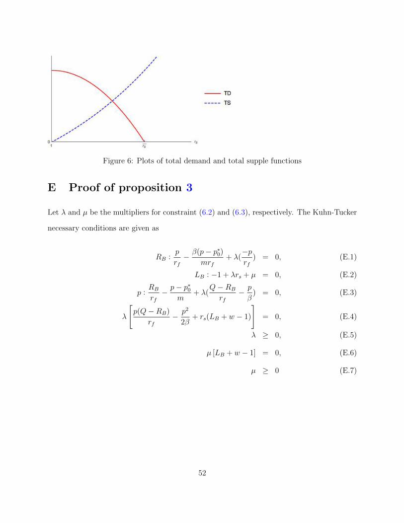
Figure 6: Plots of total demand and total supple functions

E Proof of proposition 3

Let λ and µ be the multipliers for constraint (6.2) and (6.3), respectively. The Kuhn-Tucker

necessary conditions are given as

RB :p

rf− β(p− p∗0)

mrf+ λ(

−prf

) = 0, (E.1)

LB : −1 + λrs + µ = 0, (E.2)

p :RB

rf− p− p∗0

m+ λ(

Q−RB

rf− p

β) = 0, (E.3)

λ

[p(Q−RB)

rf− p2

2β+ rs(LB + w − 1)

]= 0, (E.4)

λ ≥ 0, (E.5)

µ [LB + w − 1] = 0, (E.6)

µ ≥ 0 (E.7)

52

The first step is to prove that constraint (6.3) is binding. If not, then µ = 0, and λ = 1rs

from (E.2). Replacing λ in equations (E.1) and (E.3) and solving for p and RB yields

p∗ =β

β +m( 1rs− 1)

p∗0,

R∗B =(1− 1

rs)(β + m

rs)

β(2− 1rs

)−m(1− 1rs

)2Q.

As λ > 0, the constraint (6.2) must bind, which derives the optimal loan volume:

L∗B =

p2

2β− p(Q−RB)

rf

rs+ 1− w. (E.8)

Since L∗B > 1 − w, one must have p∗

2β>

Q−R∗B

rf, that is, β

m< 2(1 − 1

rs) < 2. But we require

that m < β2, contradiction. Therefore, constraint (6.3) is binding and L∗B = 1− w.

The next step is to calculate the optimal loan return R∗B and monitoring effort p∗.

Assuming constraint (6.2) is not binding, then λ = 0. Furthermore, R∗B and p∗ are solved

from (E.1) and (E.3) as

R∗B =β

2β −mQ, (E.9)

p∗ =β

β −mp∗0 =

β2

(2β −m)rfQ. (E.10)

Moreover, constraint (6.3) is verified to be no binding by replacing R∗B and p∗ into (6.3).

At last, substituting the optimal value of L∗B, R∗B and p∗ into equation (6.1), non

negative profit of the bank requires that w ≥ 1− βQ2

2(2−mβ

)r2f= wN .

53

F Proof of Lemma 5

I first prove that the lender firm’s profit is lower than that of benchmark, that is, πSF < πOBF .

The lender firm’s profit πSF is a function of rs, and rs ∈ [rs(w), rs). One can get some

properties of πSF :

πSF (rs) = πOBF ,

∂πSF∂rs

(rs = rs) =

(m− β)[β2Q2 − 2(2β −m)(1− w)r2

f

] [β2Q+ (β −m)

√β2Q2 − 2(2β −m)(1− w)r2

f

](2β −m)

(β2 +m2 − βm

)βQr2

f

< 0,

limrs→+∞

∂πSF∂rs

> 0,

∂2πSF∂r2

s

=β3Q2

(β2 +m2 − βm

) (4m4 − βm3(rs + 12) + β2m2(5rs + 14)− 3β3m(3rs + 2) + 6β4rs

)r2f

(m2 − βmrs + β2(2rs − 1)

)4 > 0

So πSF is a convex function on rs ∈ [rs,+∞). Furthermore, one can compute the value of

derivative of∂πSF∂rs

at rs and get∂πSF∂rs

(rs = rs) < 0. So πSF is a decreasing function of rs on

rs ∈ [rs, rs], then one should have πSF ≤ πSF (rs = rs) = πOBF .

Next, I prove that the borrower firm’s profit is also lower than that of benchmark,

that is, πMF < πOBF . Note that the profit of benchmark πOBF = πMF (RS = 0), so the proof

of πMF < πOBF is equivalent to the proof that∂πMF∂RS

< 0. As the profit of borrower firm is

πMF = p(Q−RB−RS)rf

, taking the derivative w.r.t RS gives∂πMF∂RS

= − prf

+ Q−RB−RSrf

∂p∂RS

. In the

equilibrium, one has frac∂p∂RS < 0, since shadow bank loan replaces bank loan, but bank

provides monitoring which increases p but shadow bank does not monitoring, so the increase

of shadow bank loan reduces bank monitoring and results in lower success probability p.

Overall,∂πMF∂RS

< 0, so πOBF = πMF (RS = 0) > πMF .

54

G Proof of Lemma 7

Replacing the optimal entrepreneur effort p∗, one gets the Lagrangian problem as

L =β(Q−RS)RS

r2f

− LS + λ

[β(Q−RS)2

2r2f

+ LS + w − 1

]+ µ(LS + w − 1),

where λ is the multiplier of constraint (6.12) and µ is the multiplier of constraint (6.13).

Taking derivative with respect to LS and RS respectively, yields

∂L∂LS

= −1 + λ+ µ, (G.1)

∂L∂RS

=β(Q− 2RS)

r2f

− λβ(Q−RS)

r2f

. (G.2)

Assuming constraint (6.13) binds, so L∗S = 1 − w and one needs µ > 0. Further, assuming

(6.12) also binds, then one should have R∗S = Q, which contradicts with the requirement that

RS < Q. So (6.12) does not bind, then one gets λ = 0. Equation (G.2) gives the optimal

shadow bank return R∗S = Q2

. Substituting λ = 0 into equation (G.1), one gets µ = 1 > 0,

which confirms the assumption that constraint (6.13) indeed binds. At last, replacing the

optimal values of L∗S and R∗S into shadow bank constraint (6.14), one gets w ≥ wS.

H Proof of Lemma 8

First proving that the equilibrium expected rate of return rs is an increasing function of q.

Taking q2 > q1 > 0, suppose rs is not increasing function of q, then one should have either

rs(q2) > rs(q1), or rs(q2) = rs(q1). In the first case, assuming rs(q2) > rs(q1). Since TD

is a decreasing function of rs, one gets TD(rs(q2)) > TD(rs(q1)). One the other hand, T S

is an increasing function of rs, so one gets T S(rs(q2)) < TS(rs(q1)). By the definition of

rs, one should have TD(rs(q1)) = T S(rs(q1)), and TD(rs(q2)) = T S(rs(q2)). But we have

55

T S(rs(q2)) < TS(rs(q1)) = TD(rs(q1)) < TD(rs(q2)), which is a contradiction. In another

case, assuming rs(q2) = rs(q1), one should have T S(rs(q2)) = T S(rs(q1)). But T S is an

decreasing function of q, so T S(q2) < TS(q1), which is again a contradiction. Therefore, rs

is an increasing function of q. So for any q > 0, r∗s(q) > r∗s(q = 0) = r∗s .

When q = 0, there exists an upper bound rs such that for any rs ≥ rs, the total

demand from unrestricted industries shrinks to zero, that is TD(rs) = 0. But when q > 0,

the total demand expands by the restricted industries. When rs ≥ rs, the demand from the

unrestricted industries shrinks to zero, but the demand from the restricted industries is still

positive. Hence, when q is large enough, the equilibrium rs could go above rs. In this case,

only restricted industries require shadow bank loan, which is plotted in figure 7.

Figure 7: Total demand and total supply function with restricted industries

56

I Proof of Lemma 9

First, when shadow bank does not monitor the borrowers firms, firms with low capitalization

w ∈ [wN , w1) only get bank financing. The bank loan contract is determined by the bank

zero-profit constraint, that is

p(Q−RB)

rf− mR2

B

2r2f

=(m− 2β)R2

B + 2βQRB

2r2f

= 1− w.

Solving the quadratic function of RB gives the optimal bank repayment R∗B. But when

w < wN , the determinant of the quadratic function is negative, which means there is no

solution. Intuitively, it is because when firm has low net wealth, the agency cost is very

high, so bank has to charge very high repayment, but then the entrepreneur will incur

negative utility, which is not optimal. When bank can better monitor the borrowers firms,

the entrepreneur still takes the minimum amount of loan, that is LB +LS = 1−w. To prove

that credit rationing could be alleviated, one can prove that there exists positive solution

RB and RS which solves the constraint LB + LS = 1− w.

Replacing LB with equation (6.20) and LS with equation (6.21), substituting p, one

can rewrite the constraint as a function of RB:

(m−2β)R2B+2

[βQ+ (ms − β)RS +

m− βrs

RS

]RB+

2

rsRS(βQ+(ms−β)RS)−m

2sR

2S

rs−2r2

f (1−w) = 0.

The determinant is computed as

∆ = β2Q2−2(2β−m)r2f (1−w)+2βQRS(β

rs−β+ms)+R

2S

[(ms − β +

m− βrs

)2 +2β −mrs

(m2s + 2ms − 2β)

].

Note that when w = wN , sum of the first two components results in zero. The sum of

last two components is an increasing function of ms, and when ms → β2, 2βQRS( β

rs− β

2) +

R2S

[(−β

2+ m−β

rs)2 + 2β−m

rs(β

2

2 − β)]> 0. So for large ms, the determinant ∆ is positive,

57

which means that there exists solution RB and RS which solves the constraint equation. In

other words, the bank and shadow bank can extend credit to medium-capitalized firms.

Second, the borrowers firm only takes the minimum amount of financing, that is

LB + LS = 1− w. The entrepreneur optimization problem can be simplified as

maxRB ,RS

β

2r2f

[(Q+ (

ms

β− 1)RS + (

m

β− 1)RB

)(Q− (

ms

β+ 1)RS +

2

rsRS − (

m

β− 1)RB

)− m

βR2B −

msR2S

βrs

]+w−1,

(I.1)

subject to

RB

(Q+ (

ms

β− 1)RS + (

m

2β− 1)RB

)+RSrs

(Q+ (

ms

2β− 1)RS + (

m

β− 1)RB

)≥

r2f (1− w)

β, (I.2)

RB +RS ≤ Q, (I.3)

RB ≥ 0, (I.4)

RS ≥ 0. (I.5)

Let λ, µ be the multiplier of constraint (C.2) and (I.5), respectively, one gets the Lagrangian

problem as

L =β

2r2f

[(Q+ (

ms

β− 1)RS + (

m

β− 1)RB

)(Q− (

ms

β+ 1)RS +

2

rsRS − (

m

β− 1)RB

)− m

βR2B −

msR2S

βrs

]+ w − 1

+λ

[RB

(Q+ (

ms

β− 1)RS + (

m

2β− 1)RB

)+RSrs

(Q+ (

ms

2β− 1)RS + (

m

β− 1)RB

)−r2f (1− w)

β

].

Taking derivative with respect to RB and RS respectively, yields

∂L∂RB

= (m

β−1)

[(

2

rs− 2ms

β)RS − 2(

m

β− 1)RB

]−2m

βRB+λ

[Q+ (

m

β− 2)RB + (

mβ − 1

rs+ms

β− 1)RS

]= 0

(I.6)

∂L∂RS

= 2(1

rs−1)Q+2(

ms

rsβ−m

2s

β2− 2

rs−1)RS+(

2

rs−ms

β)(m

β−1)RB+λ

[Q

rs+ (

ms

β− 1)

2RSrs

+ (

mβ − 1

rs+ms

β− 1)RB

]+µ = 0.

(I.7)

Assuming the constraint (I.2) does not bind, then λ = 0. Substituting λ = 0 into equations

(I.6) and (I.7) and solve RS as

RS =β(β2 +m2 − βm

)Q(rs − 1)rs

−β2(m((rs − 2)rs + 2) +msrs) + βm(m(rs − 1)2 + 3msrs

)−mmsrs(m+msrs) + β3(rs − 1)2

< 0,

58

which violates the constraint that RS > 0. So constraint (I.2) binds, that is, LB+LS = 1−w.

In terms of firm profit πF and success probability p. For borrowers firms, the success

probability is increased by taking shadow bank loan. Since p = βQ+(m−β)RB+(ms−β)RSrf

, taking

derivative of RS, yields ∂p∂RS

= ms−βrf

+ ∂p∂RB

∂RB∂RS

= ms−βrf

+ β−mrf

= ms−mrf

> 0. For firm profit

π, since entrepreneur utility U = π− p2

2β, the utility should increase when entrepreneur takes

shadow bank loan. On the right hand side, the increase of p causes reduction of dis-utility

− p2

2β. To have an equality, π must be increased. That is, the borrowers firms get higher

profits.

For lenders firms, the success probability p is reduced, it’s the same reasoning as

the main model part. over-borrowing from the bank increases the debt level of firms, which

reduces the entrepreneur non-monitoring effort and in the end reduces the success probability.

59

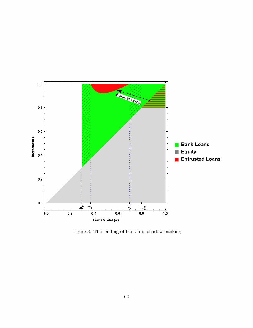
Figure 8: The lending of bank and shadow banking

60

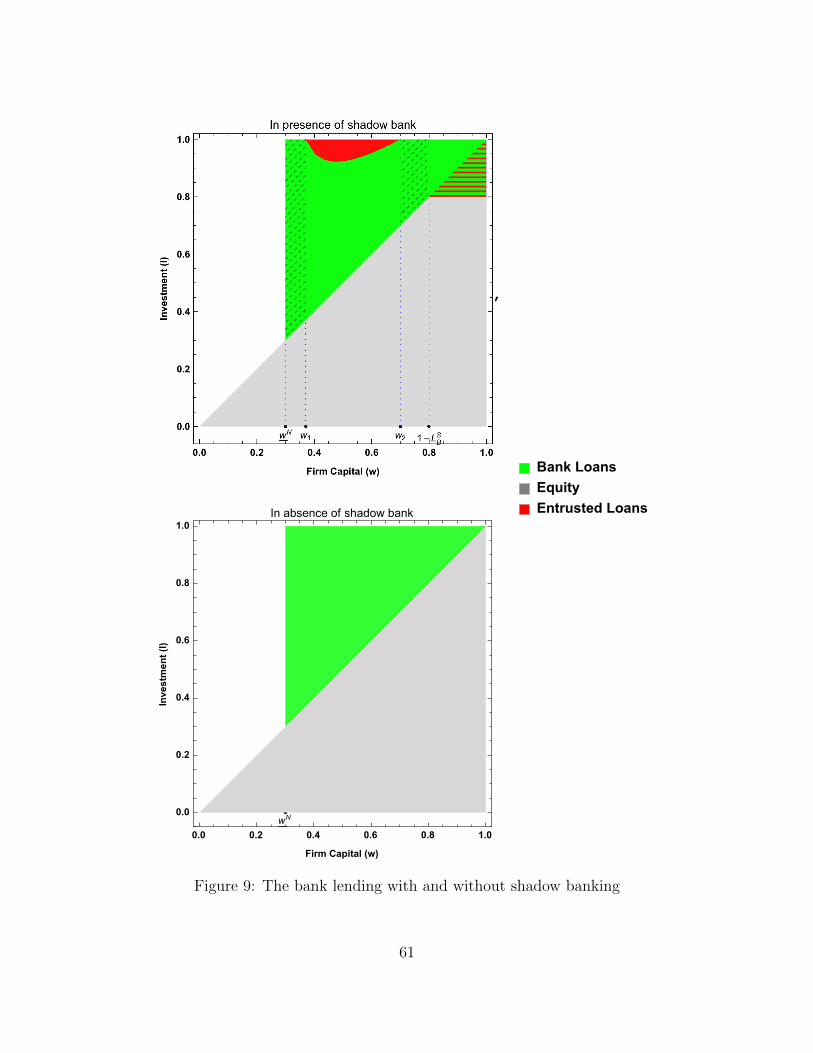
Figure 9: The bank lending with and without shadow banking

61

(a) when q = 0.03

(b) when q = 0.1

Figure 10: The bank and shadow bank lending with restricted industries

62