AN ENSEMBLE MODELING APPROACH TO EXAMINING THE …

AN ENSEMBLE MODELING APPROACH TO EXAMINING THE IMPACT OF THE

SAHARAN AIR LAYER ON THE EVOLUTION OF AN IDEALIZED TROPICAL

CYCLONE

BY

RICHARD JAMES MALIAWCO JR.

THESIS

Submitted in partial fulfillment of the requirements

for the degree of Master of Science in Atmospheric Sciences

in the Graduate College of the

University of Illinois at Urbana-Champaign, 2012

Urbana, Illinois

Advisers:

Professor Greg Michael McFarquhar

Dr. Brian F. Jewett

ii

ABSTRACT

The Saharan air layer (SAL) is a warm, dry, dusty layer of

air that resides over the tropical Atlantic Ocean. While some

studies have found that the SAL may indirectly promote tropical

cyclone (TC) development, others have identified potential

inhibiting factors for TC development. One uncertainty is

whether TC evolution depends on increases in cloud condensation

nuclei, thought to occur in the SAL, in a predictable manner. In

this study, the Regional Atmospheric Modeling System (RAMS) was

used to test if a systematic dependence of the evolution of TC

intensity on cloud condensation nuclei (CCN) concentration

exists in the context of uncertainties induced by perturbations

in other parameters describing the meteorological conditions and

properties of the initial vortex.

First, RAMSv6.0 was used to show that minor differences in

computational architecture across platforms resulted in maximum

surface wind speed, Vmax, variations of 8.1 ms-1 as early as 12

hours into simulations with identical initial conditions.

Results were identical when simulations with the same initial

conditions were conducted on the same compute node. Second,

RAMSv6.0 simulations on the same compute node examined how TC

evolution responded to changes in the initial warm bubble

temperature used to initialize convection and in the initial

radius of maximum winds (RMW) in the vortex. Two and three grid

iii

simulations assessed the importance of horizontal resolution on

the magnitude of the sensitivity to changes in these parameters.

The sensitivity was greater in the 2 grid simulations than in

the 3 grid simulations with a spread in Vmax at 96 hours of 14.4

ms-1 and 8.8 ms

-1 respectively for the RMW tests.

Finally, RAMSv4.3 was used to assess the impacts of dust

acting as CCN on TC evolution in the context of changes in other

initial conditions by conducting an ensemble of simulations. For

CCN of 100, 101, 1000 and 2000 cm-3, a series of simulations with

varying environmental temperature, relative humidity, warm

bubble temperature, vortex height, and RMW were conducted. A

monotonic relationship was seen such that the mean MSLP

increased and mean Vmax decreased with increasing CCN. Although

the difference in mean Vmax of TCs simulated with CCN

concentrations of 100 vs. 101 cm-3 was larger than one standard

deviation in the first 24 hours of simulated time, beyond 36

hours the mean values were within a standard deviation of each

other. With a few exceptions, the mean Vmax and MSLP for

simulations with CCN of 100, 1000 and 2000 cm-3 differed by more

than one standard deviation from each other. Thus, the analysis

suggests that the effect of CCN on TC intensity is greater than

uncertainties in intensity induced by non-linear amplification

of noise in the initial conditions.

iv

ACKNOWLEDGMENTS

While there are countless individuals to whom I owe my

gratitude for helping to make this M.S. thesis possible, I must

begin with a reflection. Even at the young age of 25, I have

embarked on an extraordinary journey in life. It is unfathomable

to me that I have gone from writing daily journal articles about

the weather as early as 3rd grade to now having earned my M.S.

degree in atmospheric sciences. The journey from a hobby in

weather to a dream career in meteorology is far from over, and

even getting to this point has not been without setbacks;

however, I have always carried a positive attitude and strived

to meet the challenges of the moment.

When I succeed at something I take great pride that hard

work and commitment to seeing things through has paid off. On

the other hand, when I do not quite make it through with the

strides I could have hoped for, I take comfort in the fact that

I have learned a great deal from having attempted a challenge

rather than walking away. While figuring out the things one is

talented at and what one wants to do in life are important, also

finding out what isn’t quite the right fit can also be

incredibly beneficial. A rigorous graduate program in

atmospheric sciences at the University of Illinois at Urbana-

Champaign combined with an incredible support team who believed

v

in me even when times were tough have enabled me to make my

experiences here remarkably rewarding. I have not only been able

to affirm that a career in meteorology is a perfect fit for me,

but I have also learned a great deal about my strengths and

weaknesses and I am certain this will be important to ensuring a

long-term career upon graduation. As a result, there are

countless to whom I am thankful.

I must first express my warmest heartfelt thank you to my

advisor, Greg McFarquhar. As an undergraduate at Lyndon State

College I made initial contact with him to express an interest

in his research and the program here. I made it known that I was

very passionate and motivated and that I wanted to acquire a

deeper understanding of atmospheric science principles. While I

had dreamed of becoming a weather forecaster someday, I realized

that the landscape was competitive. I knew that a master’s

degree would enhance my career opportunities and enable me to

dabble into other areas within the field such as research. I

also wanted a chance to better myself at a skill that has fought

with me tooth and nail as an undergraduate, computer

programming. And even though I was not an all-star student with

a 4.0 GPA or ideal graduate record exam (GRE) scores, Greg took

me in under his wing and gave me the opportunity I desired.

There have been a number of positive benefits as a result

of my experiences here. I had the opportunity to travel around

vi

the country to present at conferences (29th Conference on

Hurricanes and Tropical Meteorology at Tucson, AZ & the 13th

Conference on Cloud Physics in Portland, OR). Having been a part

of an exciting project, I even considered continuing on for a

Ph.D. for a time. While in Ft. Lauderdale however, I gathered

forecasting experience between 03 and 18 September 2010 as part

of NASA’s Genesis and Rapid Intensification Processes (GRIP)

field campaign. That reaffirmed to me my passion for operational

weather forecasting. Beyond this, while I was delighted to have

the opportunity to work on computer programming skills, I

continued to struggle, and I realized more and more that a

career involving this skill set was not the right match for me.

However, it was my advisor, Greg, who upon coming here to UIUC,

has helped me to figure that out. That is because he quite

literally gave me every opportunity in the world to succeed. For

that I am endlessly grateful. Even when I had endured very

serious personal matters in my life, Greg has always been

understanding and continued to believe in me. It seems at times

he will stop at nothing to see his students succeed, and that is

why I tremendously valued my time here, even having endured a

number of shortcomings. Greg, in more ways than he will ever

realize, has been a true inspiration to me.

vii

I would also like to thank my co-advisor Brian Jewett for

all of his support during my stay here. Without his help and

optimistic attitude, I would not be where I am today. He has

taken upon himself numerous efforts to assist me in coding and

trying to get me to overcome my struggles. He has always made

himself available when I had questions and has been a miracle

worker when it came to helping me understand modeling at a level

I never thought could be possible before coming here.

Scott Braun at NASA Goddard’s Space Flight Center in

Greenbelt, MD is also owed a tremendous thank you for providing

me with an opportunity to work for him during the summer of

2011. That summer was one of my most memorable and it was a

fantastic learning opportunity.

I would like to thank Eric Snodgrass for allowing me to be

his teaching assistant during the spring of 2012. Here I was

able to get exposure to a different aspect of the field, and I

walked away with a new found appreciation to just how much

effort goes into grading assignments and exams. I fully

understand why sometimes it took professors a week or more to

get an assignment back to me for my classes! Thank you so much

for helping me to see the light!

I also need to extend a thank you to UIUC’s Department of

Atmospheric Sciences and their computing resources staff, as

well as the San Diego Supercomputer Center (SDSC) computational

viii

resources. I must further acknowledge the NASA Hurricane Science

Program grant (GrantNNX09AB82G) for financial support.

Lastly, I would like to thank countless friends, as well as

my family, who have been there for me since day one. Whether it

has been experiencing the blizzard on my 18th birthday,

graduating high school on the first day of the Atlantic

hurricane season in 2005, starting college when Katrina entered

the Gulf of Mexico as a dangerous hurricane, or moving hundreds

of miles away to attend graduate school, my family has always

given me love, support, and encouragement to reach my dreams.

Without them, and without everyone mentioned herein, I would

never have been able to take the steps necessary to turn what

was once a childhood hobby into a remarkable career of my

dreams. With the deposition of this thesis, I become one step

closer to reaching my version of the American dream. Thank you

all from the bottom of my heart.

ix

TABLE OF CONTENTS

CHAPTER

1. INTRODUCTION.................................................1

1.1 Motivation of Study.....................................1

1.2 Overview of SAL Impacts on TC Evolution.................3

1.3 Objectives..............................................6

2. METHODOLOGY..................................................9

2.1 Description of RAMS.....................................9

2.2 Model Configuration for RAMSv6.0 Sensitivity Tests......9

2.3 Description of RAMSv6.0 Sensitivity Tests..............11

2.4 Model Configuration for RAMSv4.3 Ensemble Runs.........13

2.5 Description of Ensemble Runs Using RAMSv4.3............14

2.6 Tables.................................................15

3. RESULTS SECTION.............................................19

3.1 Discussion of RAMSv6.0 Sensitivity Tests..............19

3.2 Discussion of RAMSv4.3 Ensemble Runs...................28

3.3 Figures................................................37

4. CONCLUSIONS & FUTURE WORK...................................62

4.1 Concluding Remarks.....................................62

4.2 Future Plans...........................................64

REFERENCES..................................................67

1

CHAPTER 1

INTRODUCTION

1.1 Motivation of Study

Tropical cyclones (hereafter, TCs) have been widely

studied. They are among nature’s most lethal phenomena and can

leave behind a steep price tag. TCs are often associated with

damaging winds, heavy rainfall, storm surge, beach erosion,

inland flooding, and even tornadoes. TCs are often identified as

primary causes for many societal and economic problems. These

impacts have motivated decades of research into the factors that

influence the development and evolution of TC track and

intensity. The Galveston Hurricane of 1900 claimed the lives of

more than 8000 people and is considered the deadliest TC to have

affected the U.S. More recently in 2005, Hurricane Katrina was

responsible for at least 1500 fatalities and is among the top

three deadliest TCs to impact the U.S. in recorded history

(Blake et al., 2007). Emanuel et al. (2006) described Katrina as

the single most costly natural disaster for the United States,

carrying a $125 billion price tag. The impacts of Hurricane

Mitch of 1998, responsible for 11,000 deaths in Central America

were also immense. Undoubtedly, improved TC forecasts could have

important societal and economic benefits.

Aberson (2001) discussed how numerical guidance has led to

improved hurricane track forecasts since 1976 by approximately

2

0.7% per year. However, intensity forecast improvements have not

been as robust. Poor collection of inner-core data for numerical

model assimilation, limitations in computational resources, and

lack of understanding of TC physics and environmental

interaction may all be responsible for the lag in TC intensity

forecasting improvements (Rogers et al., 2006). Davis et al.

(2010) discussed the challenges in hurricane intensity

prediction that still exist even after four decades of research

and suggested that there is a need to further investigate the

environmental and internal processes that modulate TC intensity

changes.

There are many factors that influence the development and

evolution of TCs. Gray (1968) showed that large wind shear

between 250-850 hPa inhibits TC activity in the southwestern

Atlantic and central Pacific. He also discussed the importance

of high sea surface temperatures (hereafter, SSTs) and high low-

mid tropospheric moisture on TC development and intensity.

Emanuel (2005) established that increasing SSTs linked to global

warming may partly increase average TC intensity; however,

other factors such as the decrease 250-850 hPa vertical wind

shear by approximately 0.3 ms-1 per decade from 1949-2003 may

have also played a role in increasing the average intensity of

TCs. Webster (2005) explained an upward 30 year trend of more

frequent and stronger hurricanes in the context of global

3

warming; however, he concluded that a longer global data record

is needed before 30 year trends can be attributed to global

warming. Kossin (2007) did not find increases in TC intensity

over the last 30 years in any basin other than the Atlantic.

Vecchi and Soden (2007) showed that increases in June-November

vertical wind shear across the tropical Atlantic projected by

climate models may also have implications for TC activity. Other

factors that influence TCs are related to interannual

teleconnections such as the El Niño Southern Oscillation (Pielke

and Landsea, 1999). Therefore, the effect of increasing global

SSTs on TC intensity is uncertain due to the myriad of other

factors that also affect intensity.

1.2 Overview of SAL Impacts on TC Evolution

While some studies have focused on factors that affect TC

frequency, evolution, intensity, and structure (such as the

impacts of warm SSTs, vertical wind shear, moisture and

temperature vertical profiles, etc.), more recent investigations

have begun to focus on how microphysical processes such as those

induced by potential effects of enhanced dust from the Saharan

Air Layer (hereafter, SAL), impact TC evolution. Twomey (1974,

1977) showed that increases in atmospheric cloud condensation

nuclei (hereafter, CCN) concentrations lead to increases in

cloud droplet number and a decrease in mean cloud droplet size

under conditions of constant liquid water content through what

4

is referred to as the first indirect aerosol effect. In turn,

this results in clouds reflecting more solar radiation. Albrecht

(1989) discussed the second aerosol effect where smaller cloud

droplets result in lower collision and coalescence efficiencies

and therefore inhibit the formation of large raindrops, which

leads to suppressed precipitation. These two effects could

conceivably impact TC evolution. Therefore, continuing

investigations into aerosol influences on TCs may eventually

lead to improved understanding of TC evolution and

predictability.

Carlson and Prospero (1972) performed the first systematic

study on the SAL. The SAL, a deep isentropic air layer over the

Saharan Desert, has high potential temperatures, low water vapor

mixing ratios, high aerosol concentrations, and a midlevel jet

along its southern periphery (Karyampudi et al., 1999). Studies

of SAL impacts on TCs have thus far yielded mixed conclusions

with some suggesting it may enhance the potential for TC

development and others suggesting the SAL may cause a reduction

in TC intensity. Dunion and Velden (2004) suggested that the SAL

suppressed TCs by introducing dry, stable air into the storm,

and by enhancing the local vertical wind shear and preexisting

trade wind inversion. Several studies reached similar

conclusions that the SAL can inhibit TC development. Evan et al.

(2006) identified an inverse relationship between Atlantic dust

5

and TC activity. Wu (2007) suggested that the SAL activity is

enhanced during drought when there is increased atmospheric dust

loading which may lead to the suppression of TC activity. Twohy

et al. (2009) suggested that since the Saharan dust is

hydroscopic it could serve as CCN. Rosenfeld et al. (2007)

showed that increases in CCN suppress the warm rain process and

weaken TCs through low-level evaporative cooling of cloud drops

and increased cooling due to precipitation melting. But, using

data from the NASA African Monsoon Multidisciplinary Analysis

(NAMMA, 2006), Jenkins et al. (2008) indicated that dust may

affect cloud microphysics by increasing convective activity.

Zhang et al. (2007, 2009) found that increases of CCN associated

with the SAL could induce changes in the sizes and number

concentrations of cloud droplets, changing the distribution of

latent heating in the eyewall and spiral rain bands, thus

influencing TC evolution through associated dynamical changes.

However, a monotonic response of TC intensity to CCN

concentration was not seen and TC intensities exhibited

sensitivity to the environmental conditions and to the time at

which the dust was injected.

As a result of the study by Zhang et al. (2007), Cotton and

Saleeby (2008) hypothesized that the dust impact on TCs suggests

a path toward modifying the intensity of hurricanes. Cotton and

Krall (2012) showed that ingestion of enhanced CCN

6

concentrations leads to smaller cloud droplet sizes, especially

in the outer TC rainbands, which, in turn leads to three

effects. First, there is a suppression of cloud droplet

collision and coalescence. Second, smaller particles have

reduced fall speeds which increases liquid water contents at

upper levels. Third, smaller droplets have reduced probability

to be collected by ice particles and therefore freeze. Cotton

and Krall (2012) showed that the increase in supercooled liquid

water altered the vertical heating profile of the TC and

resulted in an increase in downdrafts and therefore cold pool

enhancement, and therefore reducing the TC intensity. While some

studies suggested changes in dust and the SAL dramatically

affect TCs, Braun (2010), on the other hand, suggested the role

of SAL on TC evolution may have been overemphasized.

1.3 Objectives

The primary purpose of this study is to extend the studies

of Zhang et al. (2007, 2009) which found a non-monotonic

decrease in TC intensity with increasing CCN concentration. Due

to this non-monotonic response, it is conceivable that the

response to aerosols might be akin to response seen as a result

of small perturbations in initial conditions. Sippel and Zhang

(2008) performed MM5 ensemble simulations that revealed subtle

differences in initial conditions induced large uncertainties in

TC evolution. Therefore, aerosol effects need to be interpreted

7

in the context of other effects and processes that impact the

evolution of TCs. The ocean-atmosphere system operates

chaotically as small perturbations in initial conditions result

in increasingly large changes in the state of the atmosphere

with the passage of time (Lorenz, 1963). As such, instead of an

aerosol effect weakening or enhancing TC intensity, it is

possible that the sensitivity of TC evolution to CCN

concentration may be the result of amplification in non-linear

noise associated with perturbations in initial conditions

induced by small changes in aerosol concentrations.

Understanding the sensitivity of TCs to microphysical factors is

complicated by this nonlinear chaotic amplification of noise.

This study extends the work by Zhang et al., (2007, 2009)

by conducting an ensemble of model simulations to address

questions surrounding the effects of Saharan dust acting as CCN

on TCs in the context of how other initial model fields affect

TCs. Other factors that are known to affect the evolution of TCs

include the environmental temperature, relative humidity, the

depth and radius of maximum winds (hereafter, RMW) of the vortex

used to represent the initial disturbance, and the

characteristics of the warm bubble used to initiate convection.

This study aims to determine the extent to which the aerosol

effect is masked by the amplification of perturbations in

initial fields as previously described. In addition, the degree

8

to which model results are reproducible is examined. In the next

section, a detailed description of the model chosen for these

simulations is presented, as well as a complete overview of the

experiments designed to meet these objectives. This is then

followed by a summary of results, conclusions, and future work.

9

CHAPTER 2

METHODOLOGY

2.1 Description of RAMS

In this chapter, the methodology used for investigating the

sensitivity of TCs due to changes in initial model conditions is

presented. Additional model simulations conducted to assess the

reproducibility of the model are also described. Lastly, an

ensemble of simulations conducted to investigate the response of

TCs due to changes in CCN concentration in the context of

changes in other initial conditions is detailed.

The Regional Atmospheric Modeling System (hereafter, RAMS)

was selected for the purposes of these investigations. A

detailed overview of RAMS can be found in Cotton et al. (2003).

Since RAMS has the ability to explicitly simulate CCN activation

and includes double moment parameterization schemes for liquid

and ice microphysical parameters, its use for studying aerosol

impacts on clouds is appropriate. Additionally, the use of RAMS

allows for a comparison against the results of previous studies

that used this model to examine the impacts of Saharan dust

acting as CCN on TCs (Zhang et al., 2007, 2009).

2.2 Model Configuration for RAMSv6.0 Sensitivity Tests

It was previously discussed that Zhang et al. (2007)

identified a non-monotonic response of changes in TC intensity

to initial CCN concentration. It is reasonable to question

10

whether chaotic behavior (Lorenz, 1963), namely amplification of

non-linear noise associated with small perturbations in initial

conditions, may have played a role in those results. Using

RAMSv6.0, released in January of 2006, a series of model

sensitivity tests was designed in order to investigate this

possibility. The model configuration and setup for these

simulations is summarized in Table 1. The model setup mimicked

the earlier Zhang (2007, 2009) studies as closely as possible so

that the results of the different studies can be compared. The

setup consisted of a parent domain and two inner nests with

horizontal grid spacing of 24 km, 6 km, and 2 km, respectively.

The domain center was placed at 15º N latitude and 40 º W

longitude. There were 40 vertical levels which extended from the

surface to 30 km. The vertical resolution varied from 300 m near

the surface increasing to 1 km near the domain top.

The vortex used to initialize the RAMSv6.0 simulations used

an axisymmetric mesoscale convective vortex (MCV) similar to

that of Montgomery et al. (2006). The initial vortex

characteristics included a maximum tangential velocity of 6.63-

ms-1, 8 km depth, and a 75 km radius. In order to initiate

convection, a 3.0 K temperature perturbation (warm bubble) was

placed 50 km east of the domain center.

The microphysical parameterization scheme was based upon that

of Meyers et al. (1997), which includes a large liquid droplet

11

mode and explicit CCN activation, as detailed in Saleeby and

Cotton (2004). Prognostic hydrometeors included small cloud

droplets, pristine ice, rain, snow, aggregates, graupel, hail,

and large cloud droplets.

The idealized environment in which the vortex was placed

consisted of no vertical wind shear, a constant ocean surface

SST of 29 ºC, and vertical profiles of temperature and humidity

consistent with the Jordan (1958) sounding, which is based on

the 1946-1955 mean for stations in the West Indies area. These

conditions were applied in a horizontally uniform fashion in all

domains.

The model setup only differed from the Zhang et al. (2007,

2009) studies in that the Chen and Cotton (1988) radiation

scheme was used instead of that of Harrington (1997).

Originally, the use of the Harrington radiation scheme was

planned; however, trial runs with this scheme exhibited sources

of numerical instability that could not be identified. While

accounting for condensate in the atmosphere, the Chen and Cotton

(1988) radiation scheme has a limitation in that it does not

consider whether it is cloud water, rain, or ice.

2.3 Description of RAMSv6.0 Sensitivity Tests

Using this configuration, tests were designed to examine

the sensitivity of TC evolution to perturbations in initial

conditions. These simulations were conducted on manabe, the

12

local Linux cluster maintained by the University Of Illinois

Department Of Atmospheric Sciences computing support staff. The

simulations were run in parallel, meaning that multiple

processor cores were used to perform the simulations. Since

there may be minor differences in the compilation and execution

of codes on different processors, initial tests were performed

to determine the extent to which simulations were reproducible.

Additional tests where the temperature of the warm bubble and

the radius of maximum winds (hereafter, RMW) were perturbed were

also performed. The three sets of simulations were categorized

as, and will be referred to in the results section as node

tests, bubble temperature tests, and RMW tests. These sets of

simulations are summarized in Table 2, and explained in more

detail below.

Simulations with identical initial conditions were executed

to examine the effect of the computing environment on TC

evolution. These simulations were run on ten different nodes of

manabe. For the bubble temperature tests, all initial conditions

except the temperature of the warm bubble used to initialize

convection were held constant. The warm bubble, with an 8 km

height, was placed 50 km east of the domain center with bubble

temperatures of 2.0 K, 2.9 K, 3.0 K, 3.1 K and 4.0 K. The

variations of ±0.1 K and ±1.0 K about the base value of 3 K were

used to investigate the response to smaller and larger changes

13

of the initial bubble temperature, respectively. The third suite

of sensitivity tests varied the RMW with initial values of 70

km, 74.9 km, 75 km, 75.1 km, and 80 km used, representing

variations of ±0.1 km and ±1.0 km about the base value. All of

the above sensitivity tests were run using three grids with the

finest horizontal resolution being 2 km. An additional set of

bubble temperature and RMW tests were repeated using only two

domains with the finest resolution of 6 km to determine whether

the sensitivity to these parameters depended on resolution.

2.4 Model Configuration for RAMSv4.3 Ensemble Runs

RAMSv4.3 was used to conduct the ensemble of simulations,

where the response of the TC to changes in CCN concentration in

the context of the variation of other parameters was

investigated. The RAMSv4.3 version was used for this ensemble

instead of the newer RAMSv6.0 because a more sophisticated CCN

code was available in RAMSv4.3 at the time the model simulations

were performed (Cotton, 2010, personal communication).

The same model configuration that was used for the initial

sensitivity tests with RAMSv6.0 was also used for the RAMSv4.3

ensemble. Initial tests with this code suggested that the

Harrington radiation scheme was stable in RAMSv4.3 and therefore

simulations with this scheme were performed. These simulations

were conducted using single processors on the supercomputer,

14

Trestles, available at the San Diego Supercomputer Center

(SDSC). The configuration is summarized in Table 3.

2.5 Description of Ensemble Runs Using RAMSv4.3

Table 4 summarizes the initial conditions chosen for the

ensemble of simulations conducted with RAMSv4.3. The CCN

concentrations were varied over the range observed during NAMMA

(Slusher et al. 2007). Specifically, concentrations of 100, 101,

1000, and 2000 cm-3 were applied initially, horizontally

uniformly in all domains. The simulation with a concentration of

101 cm-3 was included to test the impact of small perturbations

in CCN on simulated storm properties. For each CCN

concentration, simulations with vortex depths of 6 km and 8km,

and RMWs of 70 km, 75 km, and 80 km were performed. The vortex

properties were the same that were used for the RAMSv6.0 tests.

The range of values selected for perturbations in the vortex

properties chosen here are consistent with airborne Doppler

observations (Reasor et al., 2005) of the pre-Dolly MCV over the

tropical Atlantic in 1996 and observations during the Tropical

Experiment in Mexico (TEXMEX; Raymond et al., 1998).

The vertical profile of the temperature and humidity

associated with the Jordan (1958) sounding was also varied for

each CCN concentration. At all vertical levels, the

environmental temperature was randomly perturbed by ± 0.1º C and

the humidity (mixing ratio) was also randomly perturbed by ± 1%

15

at each vertical level. Bubble temperatures of 2 K, 3 K, and 4 K

were also used for each CCN concentration. This represented 72

simulations for each CCN value for a total of 288 simulations.

The results of these simulations are discussed in the next

chapter.

2.6 TABLES

Vortex Radius of Maximum Winds

(RMW)

75 km

Vortex Depth 8.0 km

Maximum Tangential Velocity

(Initial)

6.63-ms-1

Bubble Temperature 3.0 K, 50 km E of vortex

center

Two-Moment Microphysics Scheme Cotton (2003)

Radiation Chen and Cotton (2008)

Table 1. Conditions used for control simulations conducted with

RAMSv6.0.

16

1. Reproducibility Tests Identical Simulations, 10

different nodes on manabe

2. Vortex Radius of Maximum Winds

(RMW)

70, 74.9, 75, 75.1 km

3. Bubble Temperature 2.0, 2.9, 3.0, 3.1, 4.0 K

Table 2. Summary of simulations conducted with RAMSv6.0.

17

Vortex Radius of Maximum Winds

(RMW)

75 km

Vortex Depth 8.0 km

Maximum Tangential Velocity

(Initial)

6.63-ms-1

Bubble Temperature 3.0 K, 50 km E of vortex

center

Two-Moment Microphysics Scheme Cotton (2003)

Radiation Harrington

Table 3. Conditions used for control simulations conducted with

RAMSv4.3.

18

CCN Values 100, 101, 1000, 2000 cm-3

Environmental Temperature Jordan, ± 0.1 ºC Perturbation (For

each CCN)

Environmental Humidity (q) Jordan ± 1% Perturbation (For each

CCN)

Vortex Depth Values 6.0, 8.0 km (For each CCN)

RMW 70, 75, 80 km (For Each CCN)

Bubble Temperature 2.0, 3.0, 4.0 K (For Each CCN)

Table 4. Summary of simulations conducted with RAMSv4.3.

19

CHAPTER 3

RESULTS SECTION

3.1 Discussion of RAMSv6.0 Sensitivity Tests

In this chapter, the results of the RAMSv6.0

sensitivity tests, including the effects of small perturbations

in initial conditions on TCs, are first discussed. Second, the

results of reproducibility tests conducted on different nodes on

manabe are given. Finally, the outcome of the ensemble of

simulations, conducted with RAMSv4.3 in order to investigate the

impact of changes in CCN concentration in the context of changes

in other initial conditions, is provided.

The local Linux cluster maintained by the University of

Illinois, manabe, was utilized for RAMSv6.0 simulations to

determine the magnitude of the response to perturbations in non-

linear conditions. Since processors on these nodes have minor

differences that may affect the way that codes are compiled and

executed, it was first necessary to carry out initial tests to

determine the extent to which the simulations were reproducible.

Ten simulations were conducted under different processor cores

in order to carry out this objective. The nodes on which these

tests were conducted are as follows: manabe25, manabe33,

manabe14, manabe34, manabe23, manabe44, manabe41, manabe45,

manabe42, and manabe46.

20

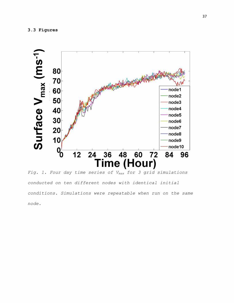
The results were identical for simulations run on manabe25

and manabe14 when comparing the binary output files of minimum

sea level pressure (MSLP) and maximum surface wind speed (Vmax).

Likewise, simulations run on manabe33, manabe45, manabe42, and

manabe46 exhibited identical results to each other. Each

additional simulation produced unique results. This describes a

total of six different solutions from ten simulations with

identical initial conditions. The 96 hour time evolution of MSLP

and Vmax is shown in figure 1. Note that there are only six lines

present because some of the simulations were identical, as

previously discussed. During the first 12 hours of simulated

time, the TC intensities ranged from 30.1 ms-1 to 38.2 ms

-1, or

differed by 8.1 ms-1; however, beyond 12 hours the spread in

solutions begins to increase. The spread in the solutions at 24

hours increased to 10.5 ms-1. The sensitivity of solutions

remained constant from about 24 hours through 84 hours, at which

time the solutions further diverged. Differences in storm

intensities between 84 and 96 hours were greater than 15 ms-1.

Within this timeframe, the strongest TC intensities exhibited

Vmax values greater than 80ms-1, while the weakest TC intensities

exhibited Vmax values around 65ms-1. As an example, at 92 hours of

simulation time, intensities varied from 65.9 to 82.5 ms-1, or

ranged by 16.6 ms-1.

21

Another way to quantify TC intensity is through the minimum

sea level pressure (MSLP). Figure 2 shows the evolution of MSLP

over the same 96 h period. Again, there were six unique

solutions for MSLP for the ten simulations discussed above.

There was little in the way of solution variation up until about

12 hours at which time the MSLP varied by 2.5 hPa, ranging from

999.9 hPa to 1002.4 hPa. Thereafter, the solutions diverged

more. By 24 hours, the sensitivity more than doubled and reached

6.4 hPa, ranging from 982.3 hPa to 988.7 hPa. The sensitivity

remained similar through about 72 hours at which time the spread

in solutions diverged further. Between 84 and 96 hours, the

simulations exhibited the largest sensitivity. At the 96 hour of

the simulations the MSLP values ranged by 8.6 hPa or from 930.0

hPa to as high as 938.6 hPa.

The simulations run on the same compute node were found to

be repeatable. Therefore, the impact of varying computer

architecture was eliminated by running all tests on the same

compute node. This strategy of conducting simulations on the

same compute node was implemented for the RWM and warm bubble

three grid and two grid sensitivity tests. Figure 3 shows the

evolution of the surface maximum wind speed with varying initial

bubble temperatures of 2.0, 2.9, 3.0, 3.1, and 4.0 K.

Through about the first 12 hours of the simulations, there

was very little in the way of sensitivity. However, by 12 hours

22

the solutions varied between 28.6 and 37.1 ms-1, or by only 8.5

ms-1. While the TCs continued to show a general intensification

trend throughout 96 hours, the rate of intensification slowed

beyond 48 hours. At 48 hours the TCs exhibited a range in

intensity of 8.3 ms-1, comparable to that of 12 hours; however,

the intensities were stronger, varying from 63.0 ms-1 to 71.3 ms

-

1. At 96 hours, the intensities ranged from 67.1 to 75.0 ms-1.

This represents a total variation of 7.9 ms-1.

There is no monotonic relationship between storm intensity

and the magnitude of the bubble temperature used to initialize

convection. The response of the TC due to changes in the warm

bubble temperature most likely just shows how non-linear noise

amplifies some small uncertainties in initial conditions.

The time evolution of MSLP for the three-grid simulations

with varying temperatures of the bubble used to initialize

convection is shown in figure 4. There is little variation in

the solutions due to changes in initial conditions through about

the first 12 hours. In fact, by 12 hours, intensity only varied

between 1000.8 and 1003.2 hPa, or by 2.4 hPa. The MSLP ranged

from about 984.0 to 989.3 hPa by 24 hours. Thus, the sensitivity

more than doubled as it increased to 5.3 hPa. However, the

spread in solutions appeared to converge again around 36 hours

(3.7 hPa variation) and again between 72 and 84 hours before

spreading out again at 96 hours. At 76 hours, the solutions

23

varied by only 1.2 hPa. At 96 hours, however, the MSLP solutions

once again exhibited larger variation the smallest value at

934.0 hPa and the weakest TC exhibiting an MSLP of 937.9 hPa.

Additional three grid simulations varying the RMW were

conducted to examine the response to other variations in initial

conditions. Figure 5 shows the evolution of the surface maximum

wind speed for simulations with initial RMW values of 70, 74.9,

75.0, 75.1, and 80.0 km. The solutions begin to exhibit notable

spread even by 12 hours of simulation time. At 12 hours TC

intensities varied between 26.1 and 37.2 ms-1, or by 11.1 ms

-1. As

the TCs intensified throughout the 4 day evolution, the

sensitivity actually exhibited decreased from that seen at 12

hours. In fact, by 48 hours of simulation time there was 8.3 ms-1

spread in TC intensities, ranging from 63.0 to 71.3 ms-1. This

sensitivity thereafter changed very little through the rest of

the simulated time. At 96 hours, the intensities ranged from

67.0 to 75.9 ms-1, representing an 8.8 ms

-1 difference. Note that

these results that are observed were similar when compared with

the warm bubble temperature sensitivity tests. The sensitivity

increased through 12 hours, and thereafter leveled off through

the remainder of the simulated time. This suggests that

amplification of noise in the initial conditions caused the

differences in these simulations seen as early as 12 hours.

24

The evolution of the MSLP is also examined to interpret the

results of the RMW tests. These results are shown in figure 6.

There was little variation as the simulations began; however,

beyond 12 hours the spread in solutions increased. At 12 hours

there was only a 1.9 hPa difference in TC intensities, ranging

from 1001.3 to 1003.2 hPa. By 24 hours, however, the spread more

than doubled to 4.2 hPa, ranging from 983.8 to 988.0 hPa. Beyond

this time period, the increase in sensitivity leveled off;

although the spread in solutions tended to decrease between 60

and 72 hours. At 68 hours of simulation time, there was only a

1.0 hPa difference in intensities, ranging from 954 to 955 hPa.

Beyond 72 hours the spread in solutions increased once again and

at 96 hours when the simulations ended the intensities ranged

from 932.2 hPa to 937.5 hPa, representing a 5.3 hPa spread.

These warm bubble temperature and RMW tests were repeated

on 2 grids in order to determine if there was a dependence of

sensitivity on the horizontal resolution of the model. Figure 7

shows the evolution of surface maximum wind speeds through 96

hours for idealized TCs initialized with bubble temperatures of

2.0, 2.9, 3.0, 3.1, and 3.0 K. As in the three grid simulations,

the solution spread diverges beyond 12 hours. At this time the

TC intensities varied between 22.2 and 26.2 ms-1 or by 4 ms

-1.

This spread amplified with time and by 24 hours the solution

spread was 4.7 ms-1 at which time TC intensities varied between

25

21.5 and 26.2 ms-1. By the end of the 96 hours of simulation

time, the TC intensities varied from 48.4 to 62.4 ms-1 or 14.0

ms-1. While the TC intensification trends are generally similar

for the two and three grid simulations, this spread is actually

larger than the 2 grid simulations, indicating that the

horizontal resolution of the simulations in fact may play a role

in the observed sensitivity in solutions.

The evolution of MSLP is summarized for the warm bubble

temperature tests simulated on two grids in Figure 8. Perhaps

one of the more notable differences in this figure is that as

compared with other tests in which the TCs appeared to intensify

at a steady rate throughout the first 36 hours before a gradual

reduction in intensification rate for the remainder of the four

days. Here, as well as for the other 2 grid sensitivity tests,

the TCs intensified initially during 12 hours, but then the

intensification leveled off until 36 hours. Beyond this the TCs

intensified again at a steady rate through 96 hours. As with the

other simulations the spread in solutions increased beyond 12

hours. The sensitivity, in general, varied little and remains at

around 4.0 hPa. At 24 hours the solutions varied between 1005.8

and 1009.7 hPa, representing a 3.9 hPa difference. In fact, even

by 84 hours the solutions varied by 4.1 hPa, or between 954.4

and 958.5 hPa. At 96 hours, however, the solutions varied

between 939.4 and 947.5 hPa, or by 8.1 hPa, almost double that

26

of only 12 hours prior. Here again, the sensitivities observed

were larger than with the three grid higher resolution

simulations.

The final sensitivity test that was conducted with RAMSv6.0

was a series of two grid simulations in which the RMW was

varied. These simulations followed a similar intensification

trend and sensitivity characteristics to that of the warm bubble

temperature sensitivity tests conducted on two grids, and are

summarized in figure 9. At 12 hours, the TC intensities varied

between 20.7 and 28.4 ms-1, or by 7.7 ms

-1. By 48 hours this

sensitivity increased to 9.1 ms-1 at which time TC intensities

varied between 31.2 and 40.3 ms-1. This spread continued to

increase, in general, throughout four days and by 96 hours was

at 14.4 ms-1 with the weakest TC having and intensity of 48.8 ms

-1

and the most intense at 63.2 ms-1. Again, this sensitivity was

larger than the three grid simulations where at 96 hours the

sensitivity for the RMW tests was observed to be 8.8 ms-1.

Lastly, the results of two grid RMW sensitivity tests

summarized in terms of the four day evolution of MSLP is shown

in figure 10. The MSLP at 12 hours exhibited a 2.7 hPa

difference, ranging from 1004.3 to 1007.0 hPa. The sensitivity

increased with time and by 48 hours was observed to be 4.9 hPa,

ranging between 991.4 and 996.3 hPa. At 96 hours the spread grew

to 13.5 hPa, ranging from 939.6 to 949.1 hPa. This spread is

27

again larger than that observed with the three grid RMW

simulations where a 5.3 hPa spread was observed at 96 hours.

This lends further support to the idea that of the degree to

which small perturbations in initial conditions amplifies is

dependent upon the horizontal resolution of the model.

In summary, the sensitivity tests conducted with RAMSV6.0

reveal the importance of considering the architecture of the

computational platforms on which model sensitivity tests are run

since TC intensities simulated on different processors can vary

by 8.1 ms-1 or 2.5 hPa even as early as 12 hours of simulation

time. Furthermore, given the uncertainties due to variations in

initial conditions observed in the warm bubble temperature and

RWM two and three grid simulations, it is reasonable to question

whether the response of TC intensity due to variations in CCN is

at least partly caused by amplification of initially small

differences in model simulations. Perhaps the furthest reaching

result from these tests is that it is important to use the same

node when conducting series of sensitivity simulations.

The next section of this chapter examines the response of

TCs to varying aerosol concentrations in the context of

responses to small changes in initial conditions by conducting

an ensemble of simulations. In doing so, this extends the

studies of Zhang et al. (2007, 2009) because it offers insight

as to whether they were seeing a physical response due to

28

variations in aerosol concentrations or merely a response of the

system to variations in initial conditions.

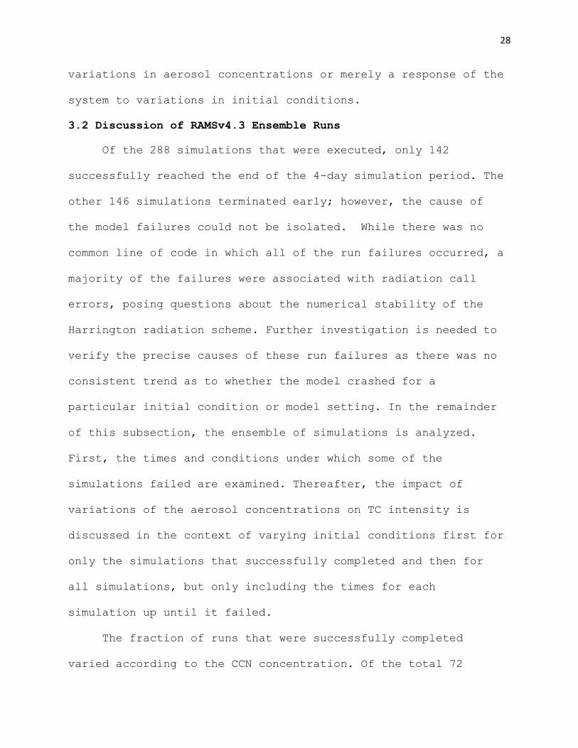
3.2 Discussion of RAMSv4.3 Ensemble Runs

Of the 288 simulations that were executed, only 142

successfully reached the end of the 4-day simulation period. The

other 146 simulations terminated early; however, the cause of

the model failures could not be isolated. While there was no

common line of code in which all of the run failures occurred, a

majority of the failures were associated with radiation call

errors, posing questions about the numerical stability of the

Harrington radiation scheme. Further investigation is needed to

verify the precise causes of these run failures as there was no

consistent trend as to whether the model crashed for a

particular initial condition or model setting. In the remainder

of this subsection, the ensemble of simulations is analyzed.

First, the times and conditions under which some of the

simulations failed are examined. Thereafter, the impact of

variations of the aerosol concentrations on TC intensity is

discussed in the context of varying initial conditions first for

only the simulations that successfully completed and then for

all simulations, but only including the times for each

simulation up until it failed.

The fraction of runs that were successfully completed

varied according to the CCN concentration. Of the total 72

29

simulations for each CCN concentration, there were a total of 55

fully completed runs with a CCN concentration of 100 cm-3, 50 for

runs with a concentration of 101 cm-3, 19 for runs with a

concentration of 1000 cm-3, and 18 for runs with a concentration

of 2000 cm-3. At this time it is unknown why the runs with higher

CCN concentration were more prone to failure.

Figure 11 shows a histogram of the time at which each of

the 288 simulations stopped. The stop time can correspond to a

natural finish (i.e., when the four day period of simulation was

completed) or when the simulations failed. There are two

clusters of times at which the model runs stopped. The highest

frequency appears at 96 hours because 142 of the 288 model runs

successfully ran for a total of four days. Although only 3 total

simulations stopped within the first 24 hours, there was a

larger cluster of model failures between 24 and 48 hours with a

total of 104 simulations having stopped by the end of 48 hours.

After 48 hours, however, there were very few model runs that

failed until beyond 78 hours.

This analysis can be separated according to the initial CCN

concentration. In figure 12, it is seen that there were only 2

runs containing a CCN concentration of 100 cm-3 that failed prior

to 48 hours. However, there were a total of 12 run failures by

48 hours. There were no additional simulations that stopped

until after 84 hours. Between 84 and 96 hours there were 2

30

additional simulations that stopped prematurely and 55

simulations finished successfully at 96 hours. Figure 13 shows

this same analysis for simulations with CCN concentrations of

101 cm-3. By 48 hours there were a total of 12 run failures;

however, 11 of them occurred after 42 hours. Beyond that run

failures occurred more slowly, and in fact by 84 hours of

simulation time there were only 3 additional simulations that

stopped prematurely. At 96 hours, 50 of the 72 runs completed

successfully, without complications. Simulations with CCN

concentrations of 1000 cm-3 failed in greater numbers, with only

19 finishing successfully at 96 hours as shown in Figure 14.

While only one failure occurred between 0 and 24 hours, the

largest number of model simulations that stopped occurred from

24 to 48 hours when an additional 39 simulations had failed.

Finally, simulations with a concentration of 2000 cm-3 exhibited

2 large clusters with greater frequency of end runtime as shown

in figure 15. It should be pointed out that with these

simulations there were no run failures during the first 24

hours. Between 24 and 48 hours there were 40 failures. While

only 3 additional simulations stopped by 84 hours, an additional

11 simulations stopped between 84 and 96 hours. Only 18

simulations were completed successfully with CCN concentrations

of 2000 cm-3.

31

This information can also be presented by displaying the

cumulative percentage of model runs that stopped as a function

of time after the model was initialized. Figure 16 shows that up

until 24 hours, only 1% of the simulations had stopped. By 48

hours, however, 36% of the simulations had stopped. Thereafter,

the rate of failure was slower with only 39% of the simulations

having stopped by 84 hours. Up to (but not including) the 96th

hour of simulation time, 45% of the total number of simulations

had stopped.

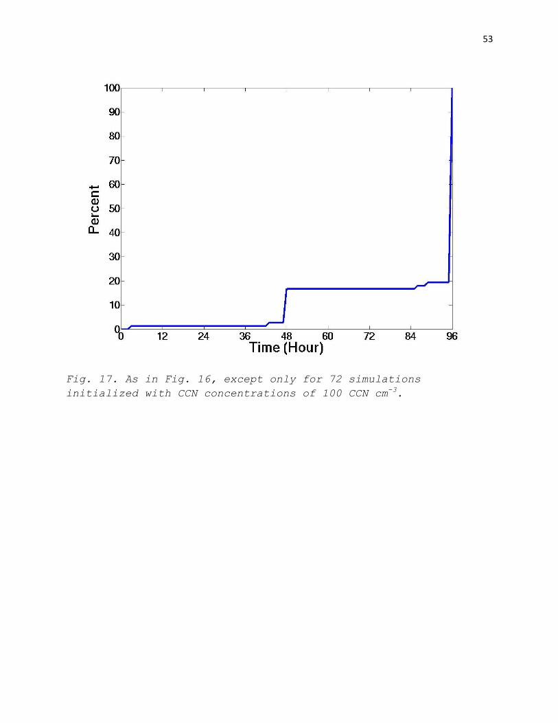
In figure 17, the cumulative frequency of the percentage of

runs stopping as a function of time for simulations conducted

with an initial CCN concentration of 100 cm-3 is shown. Through

the first 42 hours, only 1% of the model simulations had failed.

However, at 48 hours there was a sharp increase in the number of

model simulation failures since by that time 17% of the model

simulations had stopped. From 48 hours to just prior to 96

hours, the percent of model runs that stopped increased slowly

and reached 19% within the final hour of simulation time. Figure

18 shows the cumulative percent of runs that have stopped for

simulations with a CCN concentration of 101 cm-3. Just 3% of runs

failed before 48 hours, but this rises sharply to 17% after 48

hours. This value rises to 19% just prior to the 96 hour of

simulation time. The remaining 81% of simulations finished at

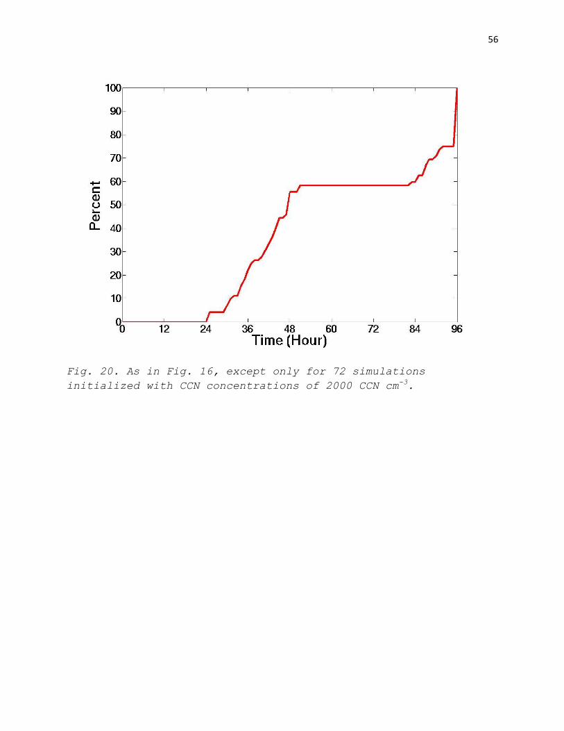
the end of the simulated time. Figure 19 shows that the

32

cumulative percent distribution of simulations with CCN

concentrations of 1000 cm-3 stopping as a function of simulation

time looks different in that from 24 to 48 hours, the percent of

runs that failed gradually increases from 0% to 56% by 48 hours.

Thereafter few runs failed until the remaining model runs

finished at 96 hours. Lastly, figure 20 shows the cumulative

percent distribution of stopped runs for all model simulations

with a CCN concentration of 2000 cm-3. While none of these

simulations fail before 24 hours, there is a steady rise in the

number of runs that failed beyond that, and by 48 hours

approximately 56% of the simulations had stopped. This value

does not increase again until 84 hours. By about 90 hours nearly

80% of the simulations had failed. The remaining 18 simulations

were successfully completed at 96 hours.

Figure 21 shows the mean surface wind speed, Vmax, computed

for simulations of each CCN concentration along with the

standard deviation (shaded) and excluding all of the model

simulations that failed prematurely. Throughout almost the

entire four day period, there was a monotonic response in Vmax to

changes in aerosol concentrations. This result differs from the

Zhang et al. (2007, 2009) studies in that they found a non-

monotonic response of Vmax to CCN concentration. This suggests

that the response of the idealized TC to variations in CCN is

stronger than the variations that occur due to non-linear

33

amplification of noise in the initial conditions. It is

important to realize that Zhang’s initial studies solely looked

at changing CCN concentrations and not many of the other factors

considered in this study.

Simulations with initial CCN concentrations of 100 and 101

cm-3 were performed to test the magnitude of response to a small

change in CCN. Through the first 24 hours, the difference in

average Vmax of TCs simulated with initial CCN concentrations of

100 vs. 101 cm-3 was larger than one standard deviation. Beyond

36 hours, the Vmax for simulations initialized with CCN

concentrations of 100 and 101 were within one standard deviation

of each other. However, it is important to note that while the

standard deviations overlapped occasionally, as discussed, the

mean value of Vmax decreased with increasing CCN at all times.

Between 24 and 60 hours the differences between the 1000 and

2000 cm-3 simulations were mostly within a standard deviation of

each other and then the solutions diverge through 96 hours with

the weaker TCs associated with higher CCN concentrations.

The four day evolution of MSLP is plotted in Figure 22,

where the mean MSLP and standard deviation for all simulations

that successfully terminated at 96 hours for each CCN

concentration is plotted. There were essentially two different

clusters of solutions after 24 hours up until 96 hours. The

simulations with 1000 and 2000 cm-3 CCN initially consistently

34

remained within one standard deviation of each other, with the

mean MSLP crossing repeatedly. The 100 and 101 cm-3 solutions

remained outside of one standard deviation of each other through

the first 36 hours; however, from 36 to 96 hours the average

MSLP for the two families were within one standard deviation of

each other. But, the mean MSLPs crossed less than those of the

1000 and 2000 cm-3 simulations. While it is unclear why there was

more overlap in the solutions of mean MSLP as compared with Vmax,

it is clearly seen that the simulations with higher

concentrations of CCN were persistently weaker when compared

with those of lower CCN concentrations.

To assess the potential importance of the failed runs on

the findings, the analyses presented in figures 21 and 22 were

repeated to include results from all model simulations up until

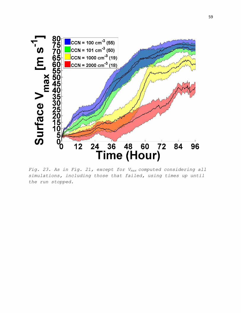
the time they stopped. Figure 23 shows the four day evolution of

mean Vmax and its standard deviation sorted according to the

initial CCN concentration. A monotonic response in Vmax to

changes in CCN concentration was again seen. The reliability of

the results will be less questionable if the same trends hold,

and in fact generally that is the case. Not only did these

results hold up, but the 100 and 101 cm-3 concentration

simulations stayed within a standard deviation again beyond 36

hours. Additionally, while the 1000 and 2000 cm-3 concentration

simulations remained within a standard deviation occasionally

35

through the first 48 hours, it was observed as before that the

means never crossed. Again the weaker TCs were associated with

the highest CCN concentrations. The most notable difference from

the analysis considering only the runs that successfully

finished is that the 1000 cm-3 simulations were considerably

weaker beyond 48 hours when failed runs were excluded; however,

the solutions were still more than one standard deviation away

from those conducted with 2000 cm-3 CCN concentrations initially,

and the overall conclusions made previously remain intact. This

is shown more clearly when the results are placed side by side

in figure 24.

Lastly, the four day evolution of mean MSLP and standard

deviation separated by CCN concentration for all runs up until

the time at which they stopped is shown in Figure 25. The same

conclusions that were obtained when the failed runs were not

included still hold. The solutions essentially diverged into two

clusters beyond 24 hours and remained as such through 96 hours.

However, unlike the Vmax analyses, the means of the MSLP plots

did occasionally cross as seen in Figure 23; however, the lower

CCN concentration simulations remained persistently stronger

than that of higher CCN concentrations. The most notable

difference is that when the failed runs were included, the 1000

cm-3 concentration simulations were somewhat more intense as

compared to when they were not included. This is consistent with

36

what was seen in Figure 23 and is particularly noted between 48

and 72 hours where the solutions between 1000 cm-3 and 2000 cm

-3

concentration simulations diverged. That phenomenon does not

occur when the failed runs were excluded.

The next chapter summarizes the main conclusions derived

from these results in context of the findings from previous

studies. It also provides implications on what these results may

mean surrounding the impacts of the SAL on TCs. There remain

many unanswered questions as a result of this study and

furthermore, there may be a need to rerun simulations to obtain

a more robust dataset where the entire ensemble of simulations

is run successfully for four days. Suggestions for further

investigation are also presented in the next chapter.

37

3.3 Figures

Fig. 1. Four day time series of Vmax for 3 grid simulations

conducted on ten different nodes with identical initial

conditions. Simulations were repeatable when run on the same

node.

38

Fig. 2. Four day time series of MSLP for 3 grid simulations

conducted on ten different nodes with identical initial

conditions. Simulations were repeatable when run on the same

node.

39


conducted on the same node with varying warm bubble temperature

perturbations used to initialize convection.

40




41


conducted on the same node with varying RMW perturbations in the

vortex used to initialize the TC.

42




43




44


conducted on the same node with varying warm bubble


45




46




47

Fig. 11. Histogram of frequency of occurrence of end runtime

sorted into 6 hour bin widths for all 288 simulations.

48

Fig. 12. As in Fig. 11, except for only simulations initialized

with CCN concentrations of 100 CCN cm-3.

49



50



51



52

Fig. 16. Cumulative percentage of all 288 simulations stopping

before the time indicated on horizontal axis.

53

Fig. 17. As in Fig. 16, except only for 72 simulations

initialized with CCN concentrations of 100 CCN cm-3.

54



55



56



57

Fig. 21. Mean Vmax (solid line) for simulations initialized with

indicated CCN concentration as a function of simulation time for

all 142 successfully completed simulations. Shading denotes one

standard deviation about the mean with following color scale

based on initial CCN concentration: 100 cm-3 (blue), 101 cm

-3

(green), 1000 cm-3 (yellow), and 2000 cm

-3 (red).

58

Fig. 22. As in Fig. 21, except for MSLP.

59

Fig. 23. As in Fig. 21, except for Vmax computed considering all

simulations, including those that failed, using times up until

the run stopped.

60

Fig. 24. A comparison of 48-96 hour time series of mean Vmax for

all simulations including the failed runs up until the model

runs stopped (left) and for the 142 successfully completed runs

(right) separated by CCN concentration. Shading denotes one

standard deviation about the mean value for the following

initial CCN concentrations: 100 cm-3 (blue), 101 cm

-3 (green),

1000 cm-3 (yellow), and 2000 cm

-3 (red).

61

Fig. 25. As in Fig. 23, except for MSLP.

62

CHAPTER 4

CONCLUSIONS & FUTURE WORK

4.1 Concluding Remarks

Previous studies have hypothesized that one of the

mechanisms by which the Saharan Aerosol Layer (SAL) can impact

tropical cyclones (TCs) is through the action of dust as cloud

condensation nuclei (CCN). In this investigation, a series of

idealized simulations were performed with the Regional

Atmospheric Modeling System (RAMS) version 6.0 to examine the

reproducibility of simulations running on different

computational nodes and to sensitivity of TC evolution to small

perturbations in the warm bubble temperature and the radius of

maximum winds (RMW) used to initialize convection. Thereafter,

RAMSv4.3 was used to conduct a series of ensemble simulations

with inner domain resolutions of 2 km allow an initial vortex to

evolve for 4 days where different ensemble members varied

initial CCN concentrations of 100, 101, 1000, and 2000 cm-3 in

the context of changes in initial conditions input into the

model. Overall conclusions from all of these simulations are

discussed in this chapter.

First, the series of simulations conducted using RAMSv6.0

with identical initial conditions on different processor cores

showed that model solutions were different depending on the

choice of node. This occurred due to minor differences in the

63

computational architecture across platforms. By simply running

on different nodes, simulations produced TCs with intensity

spreads by as much as 8.1 ms-1 or 2.5 hPa as early as 12 hours

into simulation time. When experiments were repeated on the

same node, however, the results were identical. This has

important implications for the conduct of sensitivity studies in

that series of simulations should be conducted on isolated nodes

so that the response to changes in initial conditions or

parameterization schemes is isolated from responses due to

changes in architecture.

The second series of sensitivity tests involved 2 and 3

grid simulations on RAMSv6.0 to examine how large and small

perturbations in the initial RMW and the temperature of the warm

bubble used to initialize convection affected TC evolution. By

about 12 hours of simulation time, lasting throughout the

remainder of the 96 hour runs, the response to perturbations was

observed to be largely amplification of non-linear noise. While

the storms intensified overall throughout 96 hours, there were

notable differences in the spread of the sensitivity, namely

that in general, two grid simulations tended to have a greater

range in intensities. For example, the spread at 96 hours for

two grid RMW tests was calculated to be 14.4 ms-1 which compared

to the three grid RMW tests where the spread was observed to be

8.8 ms-1.

64

The third series of sensitivity tests conducted using

RAMSv4.3 involved an ensemble of simulations designed to study

the impacts of dust acting as CCN on TCs in the context of

uncertainties induced by variations in other initial conditions.

This extends the studies by Zhang et al. (2007, 2009) which

looked at only at the effect of changing CCN centration on TCs.

Because those studies found a non-monotonic response of TC

intensity to increases in CCN concentration, it was hypothesized

that the non-linear amplification of perturbations in initial

conditions observed in the RAMSv6.0 experiments might mask an

aerosol effect on TCs. It was observed throughout the 96 hour

evolution that as CCN concentration increased, the intensity of

the TCs decreased. It is also important to note that of the 288

simulations planned, only 142 were completed in full while 146

had stopped prematurely due to unidentified causes. While this

did not appear to affect the mean results, the simulations with

1000 cm-3 were weaker beyond 48 hours when including the failed

runs in the analysis for times up until the model runs stopped.

However, any differences induced by including the failed runs

were not large enough to affect the monotonic relationship found

between changing CCN concentrations and a decrease in TC

intensity. These findings lend support to the idea that the dust

in the SAL may play an important role in the evolution of TCs.

4.2 Future Plans

65

While this study suggests that there is a physically-based

impact of changing aerosol concentrations on TC intensity, it is

important to note that there was a spread in solutions for a

constant CCN both in the ensemble of simulations conducted with

RAMSv4.3 with varying initial conditions and in the sensitivity

simulations conducted with RAMSv6.0. Because only 142 of the

planned 288 ensemble simulations with RAMSv4.3 completed

successfully, it will be necessary to reproduce these

simulations without failures. It needs to be determined whether

the numerical instability was due to the Harrington radiation

scheme or other causes to identify exactly why 146 of the 288

simulations failed.

The ensemble of simulations was conducted using a

horizontally homogenous 3-D vertical profile of CCN

concentrations at the time the TC first formed. Further

investigations should examine the effects of introducing CCN at

the TC lateral boundaries at varying stages of its evolution to

represent the situation where dust is drawn into the circulation

of a TC. Most importantly, it is necessary for the results

presented here be analyzed to investigate the physical

mechanisms by which increasing dust concentrations led to

reductions in TC intensity.

Specifically, future work will need to compare the results

to that of Cotton and Krall (2012) which showed that an

66

ingestion of enhanced CCN concentrations leads to smaller cloud

droplet sizes causing a suppression of cloud droplet collision

and coalescence, an increase in liquid water contents at upper

levels, and an increase in supercooled water which altered the

heating profile of the TC and resulted in increases in downdraft

and cold pool enhancement and therefore reducing the TC

intensity. These types of analyses and future work will begin to

enhance the physical understanding of the results obtained in

this study, the first to identify a monotonic response of

increasing CCN concentrations to a reduction in TC intensity.

67

REFERENCES

Abserson, S.D., 2001: The ensemble of tropical cyclone track

forecasting models in the North Atlantic basin (1976–2000).

Bull. Amer. Meteor. Soc., 82, 1895–1904.

Albrecht, B., 1989: Aerosols, cloud microphysics, and fractional

cloudiness, Science, 245,1227-1230.

Blake, E.S., E.N. Rappaport, and C.W. Landsea, 2007: The

deadliest, costliest, and most intense United States

tropical cyclones from 1851-2006 (and other frequently

requested hurricane facts). NOAA, Technical Memorandum NWS-

TPC-5, 43 pp.

Braun, S.A., 2010: Reevaluating the role of the Saharan air

layer in Atlantic tropical cyclogenesis and evolution. Mon.

Wea. Rev., 138, 2007-2037.

Chen, S., and W R. Cotton, 1988: The sensitivity of a simulated

extratropical mesoscale convective system to longwave

radiation and ice-phase microphysics. J. Atmos. Sci., 45,

3897–3910.

Cotton, W. R., R. A. Pielke, Sr., R. L. Walko, G. E. Liston, C.

J. Tremback, H. Jiang, R.L. McAnelly, J. Y. Harrington, M.

E. Nicholls, G. G. Carrio, and J. P. McFadden, 2003: RAMS

2001: Current status and future directions. Meteor. Atmos.

Phy., 82, 5-29.

_______, G.M. Krall, Potential indirect effects of aerosol on

68

tropical cyclone intensity, 2012: convective fluxes and

cold-pool activity. Atmos. Chem. Phy., 12, 351-385.

Davis, C., W. Wang, S.S. Chen, Y. Chen, K. Corbosiero, M.

DeMaria, J. Dudhia, G. Hollad, J. Klemp, J. Michalakes, H.

Reeves, R. Rotunno, C. Snyder, Q. Xiao, 2008: Prediction of

landfalling hurricanes with the advanced hurricane WRF

model. Mon. Wea. Rev., 136, 1990–2005.

Dunion, J. P. and C. S. Velden, 2004: The impact of the Saharan

Air Layer on Atlantic tropical cyclone activity. Bull.

Amer. Meteor. Soc., 85, 353–365.

Emanuel K., 2005: Increasing destructiveness of tropical

cyclones over the past 30 years. Nature, 436, 686-688.

______, S. Ravela, E. Vivant, and C. Risi, 2006: An statistical

deterministic approach to hurricane risk assessment. Bull.

Amer. Meteor. Soc., 87, 299 – 314.

Evan A. T., J. Dunion, J. A. Foley, A. K. Heidinger, C. S.

Velden, 2006: New evidence for a relationship between

Atlantic tropical cyclone activity and African dust

outbreaks, Geophys. Res. Lett., 33, L19813,

doi:10.1029/2006GL026408.

Gray, W.M., 1968: Global view of the origin of tropical

disturbances and storms. Mon. Wea. Rev., 96, 669-700.

Harrington J.Y., 1997: The effects of radiative and

69

microphysical processes on simulated warm and transition

season Arctic stratus. PhD. Diss., Atmospheric science

Paper No 637, Colorado State University, Department of

Atmospheric Science , Fort Collins, CO 80523, 1-289.

Jenkins, G. S. and A. Pratt (2008), Saharan dust, lightning and

tropical cyclones in the eastern tropical

Atlantic during NAMMA-06, Geophys. Res. Lett., 35, L12804,

doi:10.1029/2008GL033979.

Jordan, C. L., 1958: Mean soundings for the West Indies area. J.

Meteor., 15, 91–97.

Karyampudi, V.M., S. P. Palm, J. A. Reagen, H. Fang, W. B.

Grant, R. M. Hoff, C. Moulin, H. F. Pierce, O. Torres, E.

V. Browell, and S. H. Melfi, 1999: Validation of the

Saharan dust plume conceptual model using Lidar, Meteosat,

and ECMWF data. Bull. Amer. Meteor. Soc., 80, 1045-1074.

Kossin, J. P., K. R. Knapp, D. J. Vimont, R. J. Murnane, and B.

A. Harper, 2007: A globally consistent reanalysis of

hurricane variability and trends. Geophys. Res. Lett., 34,

L04815, doi:10.1029/2006GL028836.

Lorenz, E. N., 1963: Deterministic Nonperiodic Flow, J. Atmos.

Sci., 20, 130-141.

Meyers, M.P., R.L. Walko, J.Y Harrington, and W.R. Cotton, 1997:

New RAMS cloud microphysics parameterization. Part II: the

two moment scheme. Atmos. Res., 45, 3-39.

70

Montgomery, M. T., M. E. Nicholls, T. A. Cram and A. B.

Saunders, 2006: A “vertical” hot tower route to tropical

cyclogenesis. J. Atmos. Sci., 63, 355-386.

Pielke, R.A., C.N. Landsea, La Niña, El Niño, and Atlantic

hurricane damages in the United States (1999). Bull. Amer.

Meteor. Soc., 80, 2027-2033.

Prospero, J.M., and T.N. Carlson, 1972: Vertical and areal

distribution of Saharan dust over the western equatorial

Atlantic Ocean. J. Geophys. Res., 74, 6947-6952.

Raymond, D. J., C. López-Carrillo, and L. López Cavazos, 1998:

Case-studies of developing east Pacific easterly waves.

Quart. J. Roy. Meteor. Soc., 124, 2005–2034.

Reasor, P. D., M. T. Montgomery, and L. F. Bosart, 2005:

Mesoscale observations of the genesis of Hurricane Dolly

(1996). J. Atmos. Sci., 62, 3151–3171.

Rogers, R. F., S. Aberson, M. Black, P. Black, J. Cione, P.

Dodge, J. Gamache, J. Kaplan, M. Powell, 2006: The

Intensity Forecasting Experiment (IFEX): A NOAA multi-year

field program for improving tropical cyclone intensity

forecasts. Bull. Amer. Meteor. Soc., 87, 1523–1537.

Rosenfeld, D., Khain, A., Lynn, B., and Woodley, W. L., 2007:

Simulation of hurricane response to suppression of warm

rain by sub-micron aerosols, Atmos. Chem. Phys. Discuss.,

7, 5647-5674.

71

Saleeby, S. M., and W. R. Cotton, 2004: Large-Droplet Mode and

Prognostic Number Concentration of Cloud Droplets in the

Colorado State University Regional Atmospheric Modeling

System (RAMS). Part I: Module Descriptions and Supercell

Test Simulations. J. Appl. Meteor., 43, 182–195.

_____, Cotton, W. R.: A binned approach to cloud-droplet riming

implemented in a bulk microphysics model, J. Appl.

Meteorol., 47, 694-703, doi: 10. 1175/2007JAMC1664.1,2008.

Sippel, J. A. and F. Zhang, 2008: A probabilistic analysis of

the dynamics and predictability of tropical cyclogenesis.

J. Atmos. Sci., 65, 3440-3459.

Slusher, D. L., G. Chen, B.E., Anderson, K.L. Thornhill, E.L.

Winstead, K.J. Gleicher, G.S. Diskin, A. Nenes, 2007: The

microphysical and optical properties of Saharan dust as

observed during NAMMA. AGU fall meeting, San Francisco, CA,

December, 2007.

Twohy, C. H., et al. (2009), Saharan dust particles nucleate

droplets in eastern Atlantic clouds, Geophys. Res. Lett.,

36, L01807, doi:10.1029/2008GL035846.

Twomey, S., 1974: Pollution and planetary albedo. Atmos.

Environ., 8, 1251–1256.

______, 1977: The Influence of Pollution on the Shortwave Albedo

of Clouds, J. Atmos.Sci., 34, 1149–1152.

Vecchi, G. A. and B. J. Soden (2007), Increased tropical

72

Atlantic wind shear in model projections of global warming,

Geophys. Res. Lett., 34, L08702, doi:10.1029/2006GL028905.

Webster, P. J., G. J. Holland, J. A. Curry, and H.-R. Chang,

2005: Changes in Tropical Cyclone Number, Duration, and

Intensity in a Warming Environment. Science, 309 (5742),

1844-1846.

Wu, L. (2007): Impact of Saharan air layer on hurricane peak

intensity. Geophys. Res. Lett., 34, L09802,

doi:10.1029/2007GL029564.

Zhang, H., G. M. McFarquhar, S. M. Saleeby, and W. R. Cotton,

2007: Impacts of Saharan dust as CCN on the evolution of an

idealized tropical cyclone. Geophys. Res. Lett., 34,

L14812, doi:10.1029/2007GL029876.

______, H., G. M. McFarquhar, W. R. Cotton, and Y. Deng (2009),

Direct and indirect impacts of Saharan dust acting as cloud

condensation nuclei on tropical cyclone eyewall

development, Geophys. Res. Lett., 36, L06802,

doi:10.1029/2009GL037276.

AN ENSEMBLE MODELING APPROACH TO EXAMINING THE …

Documents

Transcript of AN ENSEMBLE MODELING APPROACH TO EXAMINING THE …