An enhanced void-crack based Rousselier damage model for...
30
This is a repository copy of An enhanced void-crack based Rousselier damage model for ductile fracture with the XFEM. White Rose Research Online URL for this paper: http://eprints.whiterose.ac.uk/135655/ Version: Accepted Version Article: Ahmad, M.I.M., Curiel-Sosa, J.L. orcid.org/0000-0003-4437-1439, Arun, S. et al. (1 more author) (2018) An enhanced void-crack based Rousselier damage model for ductile fracture with the XFEM. International Journal of Damage Mechanics. ISSN 1056-7895 https://doi.org/10.1177/1056789518802624 © 2018 The Authors. This is an author-produced version of a paper subsequently published in International Journal of Damage Mechanics. Uploaded in accordance with the publisher's self-archiving policy. [email protected] https://eprints.whiterose.ac.uk/ Reuse Items deposited in White Rose Research Online are protected by copyright, with all rights reserved unless indicated otherwise. They may be downloaded and/or printed for private study, or other acts as permitted by national copyright laws. The publisher or other rights holders may allow further reproduction and re-use of the full text version. This is indicated by the licence information on the White Rose Research Online record for the item. Takedown If you consider content in White Rose Research Online to be in breach of UK law, please notify us by emailing [email protected] including the URL of the record and the reason for the withdrawal request.
Transcript of An enhanced void-crack based Rousselier damage model for...

This is a repository copy of An enhanced void-crack based Rousselier damage model for ductile fracture with the XFEM.
White Rose Research Online URL for this paper:http://eprints.whiterose.ac.uk/135655/
Version: Accepted Version
Article:
Ahmad, M.I.M., Curiel-Sosa, J.L. orcid.org/0000-0003-4437-1439, Arun, S. et al. (1 more author) (2018) An enhanced void-crack based Rousselier damage model for ductile fracture with the XFEM. International Journal of Damage Mechanics. ISSN 1056-7895
https://doi.org/10.1177/1056789518802624
© 2018 The Authors. This is an author-produced version of a paper subsequently published in International Journal of Damage Mechanics. Uploaded in accordance with thepublisher's self-archiving policy.
[email protected]://eprints.whiterose.ac.uk/
Reuse
Items deposited in White Rose Research Online are protected by copyright, with all rights reserved unless indicated otherwise. They may be downloaded and/or printed for private study, or other acts as permitted by national copyright laws. The publisher or other rights holders may allow further reproduction and re-use of the full text version. This is indicated by the licence information on the White Rose Research Online record for the item.
Takedown
If you consider content in White Rose Research Online to be in breach of UK law, please notify us by emailing [email protected] including the URL of the record and the reason for the withdrawal request.

For Peer Review
!" #!$%$ &
'"( )%$ *%+%,*-%./ 0 ) $)) #")$ * ,' ,( ./ 0 ) $)) #,$$ * ,"./ 0 ) $)) #")$ * %, $". $)$ * / 0 )1$,
$ #
23# ), ,45*,6,0 ##"
%!
$ 36"# )# )" ! "" $ #""#3 $$7##) ""$#845*9$ " $"# "#8'9!## " $")$ 0"##0#!$#) #" ! /% %:%-/ ; ##$$"# )$6#0" $" ,$45* #$3"# )! # ,3$$"$#$0! #3 $$!# )" )$ "# ,# /%45*849"# #!$,
3$ $ 0#0 # $" !$0 )# " ")0 ##6 $ $) ! 3$45* # # ) )" "$ #"!"$ # $$4"# " $ <)# $0 #0") #"#67 # " ,3$ $$3#" ") #)# " $
http://mc.manuscriptcentral.com/ijdm
International Journal of Damage Mechanics

For Peer Review
An Enhanced Void-Crack based Rousselier Damage Model for Ductile
Fracture with the XFEM
M.I.M. Ahmada,b,c,∗, J.L. Curiel-Sosaa,b, S. Arund, J.A. Rongonga
aDepartment of Mechanical Engineering, The University of Sheffield, Sir Frederick Mappin Building, Mappin Street, S13JD Sheffield, United Kingdom
bComputer-Aided Aerospace and Mechanical Engineering Research Group (CA2M), University of Sheffield, Sheffield,UK
cDepartment of Mechanical and Materials Engineering, Faculty of Engineering and Build Environments, UniversityKebangsaan Malaysia, 43600 UKM Bangi, Selangor, Malaysia
dSchool of Mechanical Engineering, University of Phayao, Phayao, Thailand
Abstract
This work presents a modelling strategy for ductile fracture materials by implementing the Rousselier
damage model with the extended finite element method (XFEM). The implicit integration scheme and
consistent tangent modulus (CTM) based on a radial return mapping algorithm for this constitutive
model are developed by the user-defined material subroutine UMAT in ABAQUS/ Standard. To enhance
the modelling of the crack development in the materials, the XFEM is used that allows modelling of
arbitrary discontinuities, where the mesh does not have to be aligned with the boundaries of material
interfaces. This modelling strategy, so-called Rousselier-UMAT-XFEM (RuX) model is proposed to
connect both concepts, which gives an advantage in predicting the material behaviour of ductile material
in terms of voids and crack relation. This is the first contribution where XFEM is used in ductile fracture
analysis for micromechanical damage problems. The results indicate that the RuX model is a promising
technique for predicting the void volume fraction damage and crack extension in ductile material, which
shows a good agreement in terms of stress-strain and force-displacement relationships.
Keywords:
Ductile fracture, Rousselier, XFEM, crack, void damage.
1. Introduction
Materials and structures do not only deform plastically but are also subjected to damage [1]. The
internal damage variable approach defines damage as the modification of the physical properties of
materials related to irreversible growth in micro-defects [2]. Three stages occur in ductile fracture [3, 4]:
firstly, voids initiate at material defects; next, the voids enlarge where the stress triaxiality is large
due to significant plastic deformation; finally, when the voids are large enough, they coalesce to form
microcracks from which a macroscopic crack develops leading to macroscopic failure.
By considering the ductile damage caused by plastic void growth, a micromechanics based model was
developed by Gurson [5] in 1977 and phenomenologically extended in 1984 by Tvergaard and Needleman
(the so-called as GTN model) [6]. Rousselier [7, 9] then extended this model further by characterizing
the thermodynamic state with the hardening and softening of the material into the internal variables in
the framework of the plastic potential.There has been considerable research interest in the constitutive
∗Corresponding authorEmail address: [email protected] (M.I.M. Ahmad)
Preprint submitted to International Journal of Damage Mechanics July 24, 2018
Page 2 of 29
http://mc.manuscriptcentral.com/ijdm
International Journal of Damage Mechanics
1
2
3
4
5
6
7
8
9
10
11
12
13
14
15
16
17
18
19
20
21
22
23
24
25
26
27
28
29
30
31
32
33
34
35
36
37
38
39
40
41
42
43
44
45
46
47
48
49
50
51
52
53
54
55
56
57
58
59
60

For Peer Review
relations of void growth and damage for the modelling of ductile fracture. For example, Batisse et al.
[10] investigated the ductile fracture of A508 Cl 3 steel in different heat conditions based on the local
approach of fracture. In a separate study, Guo J. et al. [11] studied the ductile fracture of Al-alloy 5052
by implementing the modified Rousselier model for both tension and shear failure in a numerical and
experimental investigation. This was next followed by modelling ductile fracture over the entire range
of stress triaxiality based on classical void growth and the Mohr-Coulomb model for 6260 thin-walled
aluminium extrusion material [12].
For the extended study, it is interesting to explore the relationship of the knowledge of void ductile
damage with the crack development of the material [13]. The advanced numerical technique called
the Extended Finite Element Method (XFEM) is employed to model crack development, under the
assumptions of linear elastic fracture mechanics [14]. Since its introduction, XFEM has been developed
and used in many applications [15]. For example dynamic analysis of a stationary crack [16], failure
analysis of fibre metal laminates [17], modelling of quasi-static crack growth [18], and the analysis of
ductile damage model (Lemaitre model) for crack initiation and propagation [19].
The aim of this paper is to develop the connection between the micromechanical constitutive damage
model and crack development, in which the Rousselier-UMAT-XFEM (RuX) model is proposed and
used to represent an extensive analysis of ductile damage with a crack in the material. Indeed, this is
an exciting new achievement by implementing the XFEM solution in the constitutive Rousselier damage
model, which gives benefit in terms of the mathematical formulation to predict the void damage together
with the crack development of the ductile materials.
Accordingly, this paper is organized into five sections. An overview of the RuX model is given in
Section 2. Section 3 describes numerical frameworks, which is then followed by Section 4, which presents
the results and discussion of the study. Finally, Section 5 provides the concluding remarks of this paper.
2
Page 3 of 29
http://mc.manuscriptcentral.com/ijdm
International Journal of Damage Mechanics
1
2
3
4
5
6
7
8
9
10
11
12
13
14
15
16
17
18
19
20
21
22
23
24
25
26
27
28
29
30
31
32
33
34
35
36
37
38
39
40
41
42
43
44
45
46
47
48
49
50
51
52
53
54
55
56
57
58
59
60

For Peer Review
2. Overview of the RuX model
The RuX model solution has been proposed to predict the micromechanical damage of the material
with the existing crack development. The RuX model is a combined term of the Rousselier model
(constitutive damage model), UMAT subroutine (interface user-defined material) and XFEM solution
(crack development). Fig. 1 illustrates the flow-diagram, displaying the steps involved in the model.
Input model properties from the experimental reference
data
Prediction of material damage behaviour based on
constitutive equation
UMAT subroutine implemented within
ABAQUS/ Standard module
RuX model processing
Output:Formation of void damage, f
with a ductile crack behaviour
Figure 1: The flow diagram of RuX model
The Rousselier model was implemented using an Abaqus UMAT subroutine to describe material
damage [29]. In the subroutine, the integration scheme utilizing the radial return algorithm and implicit
solution method are formulated in the finite element method, which is explained in the next section.
Then, to introduce the crack development in the material, the XFEM solution is proposed where the
crack initiation and evolution based on the damage of traction-separation law and displacement/ energy
release rate criterion are selected for characterizing the crack behaviour.
3. Numerical frameworks
3.1. Rousselier’s Damage Model in UMAT Subroutines
The Rousselier model is a pressure-dependent plasticity model, which was developed based on the
thermodynamics of the irreversible processes (TIP) framework [12]. In the TIP framework, the specific
free energy, ψ can be defined as [7]:
ψ(
ǫeij , p, β)
= ψe(
ǫeij)
+ ψp (εeq) + ψβ (β) (1)
where ψe is elastic strain energy, ψp and ψβ are the dissipated energy relating to the mechanisms of
hardening and softening, respectively.
The Rousselier plastic potential is used to estimate the onset of yielding of the material point [8]
which shows the presence of the void volume fraction, considered as an internal state variable in the
material constitutive model. Rousselier proposed the classical plastic potential as [7, 22, 23]:
φ =q
ρ−R (εeq) +B (β)De
(
−σmρσ1
)
(2)
3
Page 4 of 29
http://mc.manuscriptcentral.com/ijdm
International Journal of Damage Mechanics
1
2
3
4
5
6
7
8
9
10
11
12
13
14
15
16
17
18
19
20
21
22
23
24
25
26
27
28
29
30
31
32
33
34
35
36
37
38
39
40
41
42
43
44
45
46
47
48
49
50
51
52
53
54
55
56
57
58
59
60

For Peer Review
where q and σm are the von Mises equivalent stress and mean stress, respectively, D and σ1 are Rousselier
material parameters, ρ is a relative density, β is an internal variable describing damage and εeq is the
equivalent plastic strain which represents hardening of the material. With loading, the void volume
fraction evolves from the initial void volume fraction, f0, of the material. The void growth rate can be
obtained as:
f = (1− f) ǫpkk = (1− f) ǫp (3)
where εpkk is the component of the plastic strain tensor.
By considering a material which contains a void, the relationship between the relative density, ρ, and
f can be written as:
ρ =
(
1− f
1− f0
)
(4)
since the value of f0 is very small compared to unity, Eq. (4) becomes as [24]:
ρ = 1− f (5)
However, f0 is still be calculated in the formulation of this study, in order to see the influence of f0 in
the formation of void growth in the material. The function of B (β) in Eq. (2) can be written in terms
of the void volume fraction as:
B (β) = σ1f (6)
By substituting Eq. (5) and Eq. (6) into Eq. (2), the Rousselier plastic potential can be written as:
φ =q
1− f−R (εeq) +Dσ1fe
(
−σm(1−f)σ1
)
(7)
Next, to implement the Rousselier model as a constitutive material in the formulation, UMAT subrou-
tine is chosen as an interface. The UMAT subroutine is the user-defined material of the ABAQUS/Standard
module, which implements the implicit integration scheme to update the state of the model and the
consistent tangent modulus (CTM) required for developing the mechanical constitutive model. For in-
tegration of the elastoplastic constitutive equation, the radial return algorithm [25, 26] is implemented
involving two main parts; the elastic predictor part, and the plastic corrector part. The detailed for-
mulation of the integration procedure is discussed further in the next section. Fig. 2 illustrates a full
schematic flow diagram of the UMAT subroutine algorithm that is implemented in this study.
4
Page 5 of 29
http://mc.manuscriptcentral.com/ijdm
International Journal of Damage Mechanics
1
2
3
4
5
6
7
8
9
10
11
12
13
14
15
16
17
18
19
20
21
22
23
24
25
26
27
28
29
30
31
32
33
34
35
36
37
38
39
40
41
42
43
44
45
46
47
48
49
50
51
52
53
54
55
56
57
58
59
60

For Peer Review
Next time increment No
Plastic regime思>0
思чϬElastic regime
START
Calculate ௧ߪ , , ௧, ௧and ݍ௧
Input the value of material properties and arrange in ordered pairs of hardening data
(E, v, ߪ௬, ߪଵ, D, , ߪ and ߝ)
Start time increment
Calculate the value of elastic properties
Set the initial value, οൌ Ͳand οൌ Ͳ
Store ߝ ௧andߪ ,Calculate the value of yield potential, 思
Update ߝ and ߪ௬Update the value of p and q
Determine the value of ο and update f
for current iteration
No [End of iteration]
Yes
Yes
No
Determine the flow direction, Update p, q, ߪ, ο , ο ߝ , and f
Calculate coefficient in Appendix C and D
Determine the CTM for current time increment
Evaluate the five constants for computing CTM for pressure dependent plasticity
model
i< maximum allowed number
Update the value of ο and οDetermine the correction value of and
Update iteration number (i=i+1)
ο or ο >
tolerance
STOP(Not converge)
Calculate coefficient in Appendix A
STOP
Yes
Figure 2: Schematic flow diagram of UMAT subroutine algorithm
3.2. Elastoplastic constitutive relations
The strain rate decomposition based on the deformation theory of plasticity [25] is formulated as:
dǫij = dǫeij + dǫpij (8)
where dǫij , dǫeij and dǫpij denote the differential change in the total, elastic and plastic strain tensors
respectively. Assuming small elastic strains, the Cauchy stress tensor, σij becomes:
σij =∂W
∂ǫeij(9)
5
Page 6 of 29
http://mc.manuscriptcentral.com/ijdm
International Journal of Damage Mechanics
1
2
3
4
5
6
7
8
9
10
11
12
13
14
15
16
17
18
19
20
21
22
23
24
25
26
27
28
29
30
31
32
33
34
35
36
37
38
39
40
41
42
43
44
45
46
47
48
49
50
51
52
53
54
55
56
57
58
59
60

For Peer Review
where W is the elastic strain energy potential. For the case of isotropic elasticity, Eq. (9) becomes:
σij = Ceijklǫ
ekl (10)
Ceijkl = 2Gδikδjl +
(
K −2
3G
)
δijδkl (11)
where Ceijkl is a fourth order elasticity tensor, G and K are the elastic shear and bulk moduli. Next, the
stress tensor in Eq. (10) can be decomposed as:
σij = σmδij + Sij (12)
where δij is the Kronecker-Delta (second order identity tensor) and Sij is the deviatoric stress component.
The elastic limit of material under the combined state of stress can be substituted by a yield function
which is expressed as:
F(
p, q,Hi)
= 0 (13)
where p = −σm is the hydrostatic pressure, q =√
32SijSij and Hi, i = 1, 2, ... is the internal state
variable such as hardening. To establish the yield criterion, the values of yield function, F are classified
as follow:
F < 0 : Elastic deformation regime (14)
F = 0 : Plastic deformation regime (15)
Hence, Eq. (12) becomes:
σij = −pδij +2
3qnij (16)
where nij =∂q
∂σij= 3
2Sij
qis the unit vector in the deviatoric space normal to the yield surface.
Moreover, to define the associated flow rule, the yield function, F and plastic potential, φ are taken
to be identical [27], and the increment in the plastic strain tensor can be written in term of the plastic
potential, φ as given by:
dǫpij = dλ∂φ
∂σij(17)
where dλ is a non-zero scalar factor of proportionality when plastic deformation occurs. The plastic
strain increment in Eq. (17) can also be decoupled into volumetric,(
dǫpij)
Vand deviatoric,
(
dǫpij)
D
parts as:
dǫpij =(
dǫpij)
V+(
dǫpij)
D
= dλ
(
∂φ
∂p
∂p
∂σij+∂φ
∂q
∂q
∂σij
)
= −1
3dλ∂φ
∂pδij + dλ
∂φ
∂qnij
(18)
6
Page 7 of 29
http://mc.manuscriptcentral.com/ijdm
International Journal of Damage Mechanics
1
2
3
4
5
6
7
8
9
10
11
12
13
14
15
16
17
18
19
20
21
22
23
24
25
26
27
28
29
30
31
32
33
34
35
36
37
38
39
40
41
42
43
44
45
46
47
48
49
50
51
52
53
54
55
56
57
58
59
60
For Peer Review
where ∂p∂σij
= −13δij and nij =
∂q∂σij
= 32Sij
q.
Substituting Eq. (18) with −dλ∂φ∂p
= dǫp and dλ∂φ∂q
= dǫq, which becomes:
dǫpij =1
3dǫpδij + dǫqnij (19)
where dǫp and dǫq are the variables corresponding to volumetric and deviatoric strain increments.
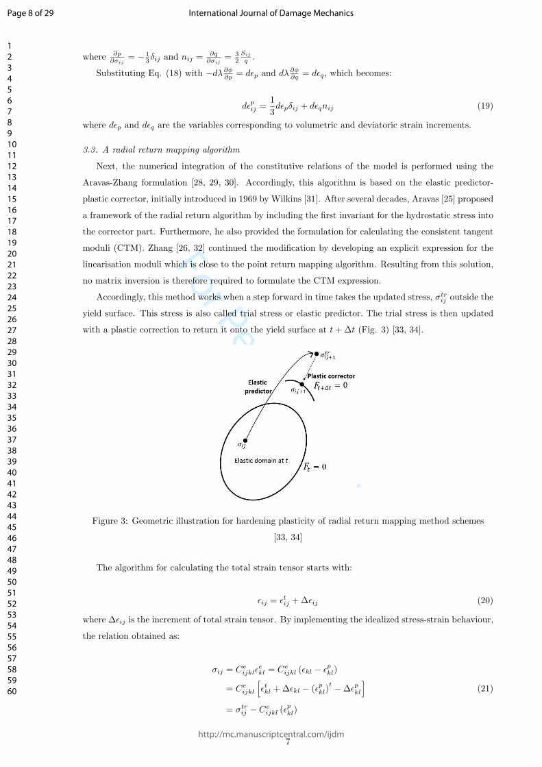
3.3. A radial return mapping algorithm
Next, the numerical integration of the constitutive relations of the model is performed using the
Aravas-Zhang formulation [28, 29, 30]. Accordingly, this algorithm is based on the elastic predictor-
plastic corrector, initially introduced in 1969 by Wilkins [31]. After several decades, Aravas [25] proposed
a framework of the radial return algorithm by including the first invariant for the hydrostatic stress into
the corrector part. Furthermore, he also provided the formulation for calculating the consistent tangent
moduli (CTM). Zhang [26, 32] continued the modification by developing an explicit expression for the
linearisation moduli which is close to the point return mapping algorithm. Resulting from this solution,
no matrix inversion is therefore required to formulate the CTM expression.
Accordingly, this method works when a step forward in time takes the updated stress, σtrij outside the
yield surface. This stress is also called trial stress or elastic predictor. The trial stress is then updated
with a plastic correction to return it onto the yield surface at t+∆t (Fig. 3) [33, 34].
Figure 3: Geometric illustration for hardening plasticity of radial return mapping method schemes
[33, 34]
The algorithm for calculating the total strain tensor starts with:
ǫij = ǫtij +∆ǫij (20)
where ∆ǫij is the increment of total strain tensor. By implementing the idealized stress-strain behaviour,
the relation obtained as:
σij = Ceijklǫ
ekl = Ce
ijkl (ǫkl − ǫpkl)
= Ceijkl
[
ǫtkl +∆ǫkl − (ǫpkl)t−∆ǫpkl
]
= σtrij − Ce
ijkl (ǫpkl)
(21)
7
Page 8 of 29
http://mc.manuscriptcentral.com/ijdm
International Journal of Damage Mechanics
1
2
3
4
5
6
7
8
9
10
11
12
13
14
15
16
17
18
19
20
21
22
23
24
25
26
27
28
29
30
31
32
33
34
35
36
37
38
39
40
41
42
43
44
45
46
47
48
49
50
51
52
53
54
55
56
57
58
59
60

For Peer Review
where ǫkl = ǫtkl +∆ǫkl, ǫpkl = (ǫpkl)
t+∆ǫpkl, σ
trij = Ce
ijkl
[
(ǫkl)t+∆ǫkl
]
is the trial stress and (ǫpkl)tis the
plastic strain tensor at time step t. The term in Eq. (21) can be further elaborated as:
Ceijkl (∆ǫ
pkl) =
[
2Gδikδjl +
(
K −2
3G
)
δijδkl
]
∆ǫpkl
= 2G∆ǫpij +K∆ǫpkkδij −2
3G∆ǫpkkδij
(22)
Subtituting Eq. (19) into Eq. (22):
Ceijkl (∆ǫ
pkl) = 2G∆ǫqnij +K∆ǫpδij (23)
Hence, Eq. (23) is used to rewrite the Eq. (21) as:
σij = σtrij − 2G∆ǫqnij −K∆ǫpδij (24)
By substituting from Eq. (16), this becomes:
−pδij +2
3qnij = −ptrδij +
2
3qtrntrij − 2G∆ǫqnij −K∆ǫpδij (25)
Thus, the correction formula for the hydrostatic pressure and equivalent stress at t+δt can be written
as:
p = ptr +K∆ǫp (26)
q = qtr − 3G∆ǫq (27)
3.4. Integrating the nonlinear equation
Following to the Newton Raphson method based on Taylor series expansion, ∆ǫp and ∆ǫq are used
to formulate the internal variables of the model as [25]:
0 = ∆ǫp
(
∂φ
∂q
)
+∆ǫq
(
∂φ
∂p
)
(28)
0 = ∆ǫpP +∆ǫqQ+ d∆ǫp
[
P +∆ǫp∂P
∂∆ǫp+∆ǫq
∂Q
∂∆ǫp
]
+ d∆ǫq
[
Q+∆ǫp∂P
∂∆ǫq+∆ǫq
∂Q
∂∆ǫq
]
+ dH1
[
∆ǫp∂P
∂H1+∆ǫq
∂Q
∂H1
]
+ dH2
[
∆ǫp∂P
∂H2+∆ǫq
∂Q
∂H2
]
(29)
where P = ∂φ∂q
and Q = ∂φ∂p
, while ∂∆ǫp and ∂∆ǫq are defined as the correction values for ∆ǫp and ∆ǫq
respectively. Moreover, the values of dH1 and dH2 can be determined as follows:
dH1 = −1
Ω
(
∂G2
∂H2
∂G1
∂∆ǫp−∂G1
∂H2
∂G2
∂∆ǫp
)
d∆ǫp +
(
∂G2
∂H2
∂G1
∂∆ǫq−∂G1
∂H2
∂G2
∂∆ǫq
)
d∆ǫq
−1
Ω
(
∂G2
∂H2
∂G1
∂p−∂G1
∂H2
∂G2
∂p
)
∂p
∂∆ǫpd∆ǫp +
(
∂G2
∂H2
∂G1
∂q−∂G1
∂H2
∂G2
∂q
)
∂q
∂∆ǫqd∆ǫq
(30)
8
Page 9 of 29
http://mc.manuscriptcentral.com/ijdm
International Journal of Damage Mechanics
1
2
3
4
5
6
7
8
9
10
11
12
13
14
15
16
17
18
19
20
21
22
23
24
25
26
27
28
29
30
31
32
33
34
35
36
37
38
39
40
41
42
43
44
45
46
47
48
49
50
51
52
53
54
55
56
57
58
59
60

For Peer Review
dH2 = −1
Ω
(
−∂G2
∂H1
∂G1
∂∆ǫp+∂G1
∂H1
∂G2
∂∆ǫp
)
d∆ǫp +
(
−∂G2
∂H1
∂G1
∂∆ǫq+∂G1
∂H1
∂G2
∂∆ǫq
)
d∆ǫq
−1
Ω
(
−∂G2
∂H1
∂G1
∂p+∂G1
∂H1
∂G2
∂p
)
∂p
∂∆ǫpd∆ǫp +
(
−∂G2
∂H1
∂G1
∂q+∂G1
∂H1
∂G2
∂q
)
∂q
∂∆ǫqd∆ǫq
(31)
where Ω =(
∂G1
∂H1
)(
∂G2
∂H2
)
−
(
∂G2
∂H1
)(
∂G1
∂H2
)
. The G1 and G2 are the functions made by regrouping the
implicit function as:
G1 = ∆H1− h1
(
∆ǫp,∆ǫq, p, q,H1, H2
)
(32)
G2 = ∆H2− h2
(
∆ǫp,∆ǫq, p, q,H1, H2
)
(33)
By implementing Eq. (30) and Eq. (31) into Eq. (29) leads to the reduced form of the Newton-
Raphson equation as:
A11cp +A12cq = b1 (34)
A21cp +A22cq = b2 (35)
where d∆ǫp = cp and d∆ǫq = cq. The derivations for Aij and bi are given in Appendix A. The value of
∆ǫp and ∆ǫq are then updated by:
∆ǫn+1p = ∆ǫnp + cp (36)
∆ǫn+1q = ∆ǫnq + cq (37)
where superscript n is the iteration number.
3.5. Static implicit solution method
In this study, the implicit method has been formulated for finite element solution from static equi-
librium and the solution is determined iteratively which is performed until a convergence criterion is
satisfied for each increment. The virtual work principle is usually employed to explain the equilibrium
state, which considers a material continuum body in volume, V and bounding surface, S subjected to
surface traction, ti and distributed body force per unit volume, fi. The equilibrium equation can be
written as [35]:
∫
S
tidS +
∫
V
fidV = 0 (38)
The Cauchy stress matrix, σij at a point on S is defined by ti = σijnj , where nj is the unit vector
outward normal to S at the point. By considering the divergence theorem of Gauss, the above equation
reduces to:
∂σij∂xj
+ fi = 0 (39)
9
Page 10 of 29
http://mc.manuscriptcentral.com/ijdm
International Journal of Damage Mechanics
1
2
3
4
5
6
7
8
9
10
11
12
13
14
15
16
17
18
19
20
21
22
23
24
25
26
27
28
29
30
31
32
33
34
35
36
37
38
39
40
41
42
43
44
45
46
47
48
49
50
51
52
53
54
55
56
57
58
59
60

For Peer Review
Multiplying Eq. (39) by a virtual displacement, δui and integrating it over the whole volume, then
applying the chain rule gives:
∫
V
σij∂δui∂xj
dV −
∫
S
tiδuidS −
∫
V
fiδuidV = 0 (40)
The term ∂δui
∂xjis the unit relative virtual displacement, which can be decomposed into the virtual
strain tensor. The equilibrium statement in Eq. (40) can be written in terms of incremental virtual
displacement, G (ui) as:
G (ui) =
∫
V
σijδǫijdV −
∫
S
tiδuidS −
∫
V
fiδuidV (41)
where σij and ǫij are conjugate of material stress and strain measures.
If the Newton Raphson method is implemented to determine a set of solutions of Eq. (41), the
estimation of the root is written as:
∆un+1i = un+1
i − uni = −
∂G (uni )
∂ui
−1
G (uni ) (42)
where superscript n is the number of iteration and∂G(un
i )∂ui
is the jacobian matrix of the governing
equations which is presented as:
∂G (uni )
∂ui= KMN =
∫
v0
Bij,MDijklBij,NdV0 + JMN (43)
where Bij,M and Bij,N are the strain variation matrices, which is based on the current position of the
material point. JMN is the global jacobian matrix and Dijkl is the consistent tangent moduli (CTM) of
the material, explained in Appendix B.
3.6. Extended Finite Element Method (XFEM)
The XFEM provides significant benefits in the numerical modelling of crack propagation where special
functions are added to the finite element approximation using the partition of unity framework [15, 36].
For crack modelling, a discontinuous function also called the Heaviside step function is where the linear
elastic asymptotic crack-tip displacement fields are used to account for the crack (Fig. 4). Therefore, this
enables the domain to be modelled by finite elements without explicitly meshing the crack surfaces. The
approximation for a displacement vector function, u with the partition of unity enrichment is [18, 37]:
u =n∑
i=1
Ni (x)ui +n∑
i=1
Ni (x)H (x) ai +n∑
i=1
Ni (x)4
∑
α=1
Fα (x) bαi (44)
where Ni (x) is the nodal shape function, ui is the nodal displacement vector associated with the con-
tinuous part of the finite element solution, H(x) associates discontinuous jump function across the crack
surfaces, ai is the nodal enriched degree of freedom vector, Fα (x) represents the elastic asymptotic
crack-tip functions and bαi is the nodal enriched degree of freedom vector. Theoretically, the first term
is applicable to all nodes in the model and the second term is for nodes whose shape function support
cross by the crack interior. Meanwhile, the third term is only for nodes crossing at the crack tip.
10
Page 11 of 29
http://mc.manuscriptcentral.com/ijdm
International Journal of Damage Mechanics
1
2
3
4
5
6
7
8
9
10
11
12
13
14
15
16
17
18
19
20
21
22
23
24
25
26
27
28
29
30
31
32
33
34
35
36
37
38
39
40
41
42
43
44
45
46
47
48
49
50
51
52
53
54
55
56
57
58
59
60

For Peer Review
The Heaviside function, H(x) across the crack surfaces gives as:
H(x) =
1 if ξ ≥ 0
−1 otherwise(45)
where ξ = n.(x − x∗), is the local axis perpendicular to the crack growth direction, x is a Gauss point,
x∗ is the point on the crack closest to x, and n is the unit outward normal to the crack at x. Moreover,
the asymptotic crack tip function, Fα (x) is given by:
Fα (x) = rm[
sinΘ
2, cos
Θ
2, sinΘsin
Θ
2, sinΘcos
Θ
2
]
(46)
where (r,Θ) is a polar coordinate system with its origin at the crack tip and m is a value which depends
on the type of material. The processes flow of XFEM formulation is presented in Fig. 5. It should be
noted that for XFEM elements, the location and the number of Gauss points between load increments
may be changed as the crack propagates. Hence, material state variables must be updated consistently
until the end of the load increment.
However, in crack propagation problems, the crack crosses over a whole element one at a time only
permitting to work on plane problems with a reduced integration element, so that the stresses and strains
are calculated in the centre of the element (on the integration point). Also, as the crack tip is never
within an element, the singularity of the stresses does not need to be considered in the definition of the
elemental displacements [39]. Moreover, the asymptotic singularity functions are only considered when
modelling stationary cracks. Therefore, the crack must propagate across an entire element to avoid
the need to model the stress singularity. Thus, in the crack propagation of plane problem, the XFEM
discontinuous displacement approximation becomes:
u =n∑
i=1
Ni (x)ui +n∑
i=1
Ni (x)H (x) ai (47)
The crack initiation and direction of the crack extension need to be defined in the XFEM formulation,
in order to simulate the degradation and eventual failure of an enriched element. The failure mechanism
consists of two concepts: a crack initiation criterion and a damage evolution law. A crack process begins
when the stresses or the strains (based on the damage of traction-separation law) satisfy specified crack
initiation criteria. After that, the damage evolution law (based on displacement or energy release rate
criterion) describes the rate at which the cohesive stiffness is degraded once the corresponding initiation
criterion is reached.
11
Page 12 of 29
http://mc.manuscriptcentral.com/ijdm
International Journal of Damage Mechanics
1
2
3
4
5
6
7
8
9
10
11
12
13
14
15
16
17
18
19
20
21
22
23
24
25
26
27
28
29
30
31
32
33
34
35
36
37
38
39
40
41
42
43
44
45
46
47
48
49
50
51
52
53
54
55
56
57
58
59
60

For Peer ReviewFigure 4: Enrichment nodes for the crack tip and the crack surfaces. The squared nodes (set of nodes
KΛ) are enriched by the crack tip functions while the circled nodes (set of nodes KΓ) are enriched by
the discontinuity functions
Start
XFEM updates• Enriched nodes and element around crack tip (asymptotic function)• Enriched nodes and elements around crack surface (heaviside function)
Crack growth criterion
XFEM formulation?
End
XFEM element integration and material point operation
Stress recovery
ABAQUS built-in element types
Penalty contact
Load increment
Contact?
Crack growth?
Yes
No
Yes
Yes
No
No
Data input and mesh initialization
Level set function
Figure 5: Flowchart of XFEM formulation [38]
12
Page 13 of 29
http://mc.manuscriptcentral.com/ijdm
International Journal of Damage Mechanics
1
2
3
4
5
6
7
8
9
10
11
12
13
14
15
16
17
18
19
20
21
22
23
24
25
26
27
28
29
30
31
32
33
34
35
36
37
38
39
40
41
42
43
44
45
46
47
48
49
50
51
52
53
54
55
56
57
58
59
60
For Peer Review
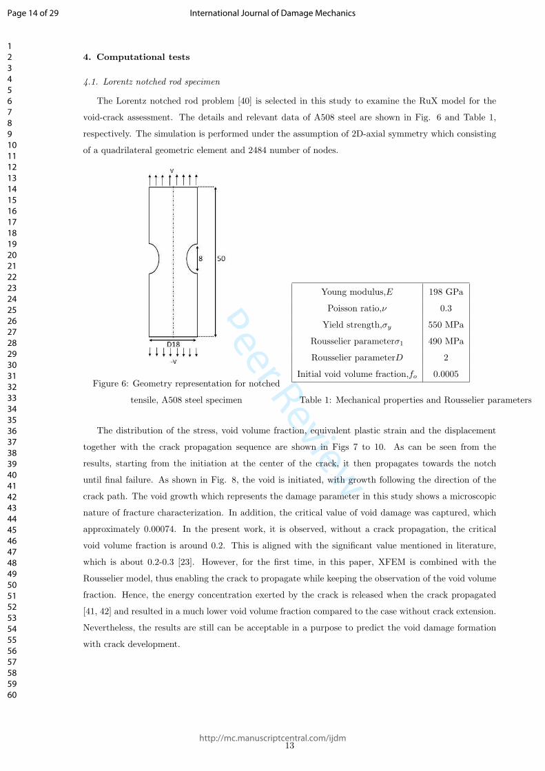
4. Computational tests
4.1. Lorentz notched rod specimen
The Lorentz notched rod problem [40] is selected in this study to examine the RuX model for the
void-crack assessment. The details and relevant data of A508 steel are shown in Fig. 6 and Table 1,
respectively. The simulation is performed under the assumption of 2D-axial symmetry which consisting
of a quadrilateral geometric element and 2484 number of nodes.
Figure 6: Geometry representation for notched
tensile, A508 steel specimen
Young modulus,E 198 GPa
Poisson ratio,ν 0.3
Yield strength,σy 550 MPa
Rousselier parameterσ1 490 MPa
Rousselier parameterD 2
Initial void volume fraction,fo 0.0005
Table 1: Mechanical properties and Rousselier parameters
The distribution of the stress, void volume fraction, equivalent plastic strain and the displacement
together with the crack propagation sequence are shown in Figs 7 to 10. As can be seen from the
results, starting from the initiation at the center of the crack, it then propagates towards the notch
until final failure. As shown in Fig. 8, the void is initiated, with growth following the direction of the
crack path. The void growth which represents the damage parameter in this study shows a microscopic
nature of fracture characterization. In addition, the critical value of void damage was captured, which
approximately 0.00074. In the present work, it is observed, without a crack propagation, the critical
void volume fraction is around 0.2. This is aligned with the significant value mentioned in literature,
which is about 0.2-0.3 [23]. However, for the first time, in this paper, XFEM is combined with the
Rousselier model, thus enabling the crack to propagate while keeping the observation of the void volume
fraction. Hence, the energy concentration exerted by the crack is released when the crack propagated
[41, 42] and resulted in a much lower void volume fraction compared to the case without crack extension.
Nevertheless, the results are still can be acceptable in a purpose to predict the void damage formation
with crack development.
13
Page 14 of 29
http://mc.manuscriptcentral.com/ijdm
International Journal of Damage Mechanics
1
2
3
4
5
6
7
8
9
10
11
12
13
14
15
16
17
18
19
20
21
22
23
24
25
26
27
28
29
30
31
32
33
34
35
36
37
38
39
40
41
42
43
44
45
46
47
48
49
50
51
52
53
54
55
56
57
58
59
60

For Peer ReviewFigure 7: Stress in y-direction along the crack
Figure 8: Void volume fraction distribution along the crack
Figure 9: Equivalent plastic strain distribution along the crack
14
Page 15 of 29
http://mc.manuscriptcentral.com/ijdm
International Journal of Damage Mechanics
1
2
3
4
5
6
7
8
9
10
11
12
13
14
15
16
17
18
19
20
21
22
23
24
25
26
27
28
29
30
31
32
33
34
35
36
37
38
39
40
41
42
43
44
45
46
47
48
49
50
51
52
53
54
55
56
57
58
59
60

For Peer ReviewFigure 10: Displacement in y-direction distribution
Next, these results were compared with the results found in the reference [40] regarding the stress
and the strain relation as shown in Fig. 11. In this figure, to trigger the connection between the damage
model with the crack or its propagation, the result from XFEM is compared with the RuX model. The
result shows that the XFEM formulation itself does not predict the behaviour in tension adequately.
However, the result for the RuX model shows an acceptable agreement with the benchmark result from
Lorentz et al. [40]. This shows that the RuX formulation connects XFEM and the damage model in
an appropriate manner. As the specimen is loaded, the stress first increases because of increasing void
fraction at the structural scale and then drops suddenly due to final cracks of the material. Numerical
values for the similarity between the predicted and benchmark results are shown in Table 2. Similarity
values of at least 95% show the effectiveness of the results in this analysis.
Table 2: Numerical values of similarity for different solution models
Solution model Total stress, (σt), MPa Similarity,%
Lorentz et al. (2008) 5957
Rousselier 6061 98
RuX 5667 95
15
Page 16 of 29
http://mc.manuscriptcentral.com/ijdm
International Journal of Damage Mechanics
1
2
3
4
5
6
7
8
9
10
11
12
13
14
15
16
17
18
19
20
21
22
23
24
25
26
27
28
29
30
31
32
33
34
35
36
37
38
39
40
41
42
43
44
45
46
47
48
49
50
51
52
53
54
55
56
57
58
59
60

For Peer ReviewFigure 11: Stress-strain curve for notched tensile specimen
This is followed by evaluating the relation between force and displacement (Fig. 12), where the force
increases with increasing displacement until it reaches final failure and then drops due to final fracture.
Figure 12: Force-displacement distribution
16
Page 17 of 29
http://mc.manuscriptcentral.com/ijdm
International Journal of Damage Mechanics
1
2
3
4
5
6
7
8
9
10
11
12
13
14
15
16
17
18
19
20
21
22
23
24
25
26
27
28
29
30
31
32
33
34
35
36
37
38
39
40
41
42
43
44
45
46
47
48
49
50
51
52
53
54
55
56
57
58
59
60

For Peer Review
Figure 13: Evolution of damage variable in Lorentz et al. [40](above) and RuX model with
crack(below)
The evolution of the void volume fraction as a damage variable between both methods is then
compared to verify the predictive capability of the RuX model (Fig. 13). It should be noted that the
benchmark model does not consider or predicts the actual crack development. The evolution begins when
the localization phenomenon occurs due to high triaxiality in the centre of the specimen (Fig. 13(a)).
The void band forms a shear band due to the influence of shear localization, and the crack initiation
occurs at the crack tip based on the damage criteria of material (Fig. 13(b)). Then the evolution is
extended as the voids coalesce along the shear bands and the crack propagates correspondingly, thereby
resulting in the bifurcation (Fig. 13(c)). Finally, the strength of the structure is lost due to final crack
or called as the ultimate fracture mode (Fig. 13(d)). Therefore, good agreement is achieved between the
simulation and the benchmark results.
However, the crack propagation in the RuX model does not show signs of any formation of the
bifurcation or cup-cone fracture at the plots like the results obtained from [40, 11]. There are some
arguments to be highlighted at this point, which is first the crack growth direction will diverge or incline
because of factors such as mesh orientation, mixed-mode loading conditions or having different material
properties due to the presence of interfaces at arbitrary orientations. In this case, a standard tension test
is simulated, and the material is considered homogeneous, thus it is impossible to form a cup-cone fracture
behaviour in the computational results. Secondly, the crack path is influenced by the arrangement of the
integration points in the elements. For this case, the crack jumps from one point to another based on
the XFEM formulation, in which the enrichment functions typically consist of the near-tip asymptotic
functions that capture the singularity around the crack tip and a discontinuous function that represents
the jump in displacement across the crack surfaces. Note that at the crack tip, where steep gradients of
17
Page 18 of 29
http://mc.manuscriptcentral.com/ijdm
International Journal of Damage Mechanics
1
2
3
4
5
6
7
8
9
10
11
12
13
14
15
16
17
18
19
20
21
22
23
24
25
26
27
28
29
30
31
32
33
34
35
36
37
38
39
40
41
42
43
44
45
46
47
48
49
50
51
52
53
54
55
56
57
58
59
60

For Peer Review
stresses and strains take place, the critical conditions for instability are achieved over some characteristic
length, related to interparticle spacing. Otherwise, void coalescence and material decohesion will not
occur [7].
4.1.1. Relative error and mesh convergence analysis
To validate the stability and accuracy of the simulation results, analysis of the relative error and
mesh convergence was conducted. The relative error is calculated from the residuals which represent
the difference between the internal and external forces acting on a model. In this case, the residual
displays information that determines whether an iteration has produced an equilibrium solution [33].
If the residuals are small, the system accepts the iteration as converged. It can be seen in Fig. 14,
from the readings that the maximum residual norm produced is consistent after 3000 iterations, showing
that the solution achieved a stable condition and the data recorded are below the tolerance value. For
this case, the tolerance is set to 0.005 and is used to determine whether a solution is converged. The
tolerances must be small to provide an accurate solution but large enough to achieve the solution within
a reasonable number of iterations [38]. Also, to identify the adequate size of meshing in the analysis, a
mesh convergence curve is presented as shown in Fig. 15, showing the convergence and reaching a stable
form [43].
Figure 14: Maximum residual norm vs. No. of iteration
18
Page 19 of 29
http://mc.manuscriptcentral.com/ijdm
International Journal of Damage Mechanics
1
2
3
4
5
6
7
8
9
10
11
12
13
14
15
16
17
18
19
20
21
22
23
24
25
26
27
28
29
30
31
32
33
34
35
36
37
38
39
40
41
42
43
44
45
46
47
48
49
50
51
52
53
54
55
56
57
58
59
60

For Peer ReviewFigure 15: Mesh convergence curve
4.2. Compact tension (CT) specimen
The RuX model is further investigated using the compact tension (CT) specimen studied by Samal
et al. [44]. A 2D-plane stress analysis test is performed consisting of the quadrilateral geometric element
and 8398 nodes used for the specimen. The geometry and the mechanical properties of the specimen
are shown in Fig. 16 and Table 3 respectively. The material of the CT specimen is low alloy steel,
22NiMoCr37 and the initial crack is 16.1 mm.
Figure 16: Geometry representation for CT-specimen
Young modulus,E 210 GPa
Poisson ratio,ν 0.3
Yield strength,σy 563 MPa
Rousselier parameterσ1 445 MPa
Rousselier parameterD 2
Initial void volume fraction,fo 0.0003
Table 3: Mechanical properties and
Rousselier parameters
The contour plots for the stress and void volume fraction are shown in Figs 17 and 18. It can be
observed from Fig. 18 that the highest void damage contour is concentrated at zones of high stress (as
shown in Fig. 17), which is at the crack tip area. Furthermore, the contour plot of plastic potential is
also presented (as shown in Fig. 19). As a final discussion point, the force, F as a function of the imposed
crack mouth opening displacement, CMOD is depicted and the comparison with the experimental result
is shown in Fig. 20. It can be seen that the RuX model result follows a similar trend to the experiment,
with reasonable agreement. However, variances occur, especially after it enters the plastic region of
material behaviour. The inability to achieve a perfect match with the experiment in this region is caused
by the interaction of XFEM module in Abaqus which by default applies a linear constitutive relationship.
19
Page 20 of 29
http://mc.manuscriptcentral.com/ijdm
International Journal of Damage Mechanics
1
2
3
4
5
6
7
8
9
10
11
12
13
14
15
16
17
18
19
20
21
22
23
24
25
26
27
28
29
30
31
32
33
34
35
36
37
38
39
40
41
42
43
44
45
46
47
48
49
50
51
52
53
54
55
56
57
58
59
60

For Peer Review
In contrast, the applied Rousselier model tries to follow the material’s plastic behaviour. As it can be seen
in the previous result in Fig. 11, applying XFEM only, resulted in a linear constitutive relationship, but
applying the Rousselier model together fixing the result, thus, it follows the material’s plastic behaviour.
Nevertheless, a fair performance is shown via the new algorithm, in which the crack propagation can be
evaluated via XFEM while it tries to maintain the plastic behaviour via the Rousselier model.
20
Page 21 of 29
http://mc.manuscriptcentral.com/ijdm
International Journal of Damage Mechanics
1
2
3
4
5
6
7
8
9
10
11
12
13
14
15
16
17
18
19
20
21
22
23
24
25
26
27
28
29
30
31
32
33
34
35
36
37
38
39
40
41
42
43
44
45
46
47
48
49
50
51
52
53
54
55
56
57
58
59
60

For Peer ReviewFigure 17: Stress in y-direction along the crack
Figure 18: Void volume fraction distribution along the crack
Figure 19: Plastic potential distribution along the crack
Figure 20: Force-CMOD for CT-specimen in simulation and experiment
21
Page 22 of 29
http://mc.manuscriptcentral.com/ijdm
International Journal of Damage Mechanics
1
2
3
4
5
6
7
8
9
10
11
12
13
14
15
16
17
18
19
20
21
22
23
24
25
26
27
28
29
30
31
32
33
34
35
36
37
38
39
40
41
42
43
44
45
46
47
48
49
50
51
52
53
54
55
56
57
58
59
60
For Peer Review
5. Conclusion
Phenomenologically, the initiation and propagation of a crack by XFEM are investigated with the
evolution of the void damage described by the Rousselier model in ductile materials. From this study,
ductile fracture analysis was successfully achieved by combining the XFEM with the Rousselier damage
model and the RuX model was introduced as a solution. This is the first contribution that practically
describes the relationship between the void volume fraction as a damage parameter with the crack growth,
which can enhance the numerical solution for the prediction of ductile fracture behaviour. There have
some points that need to be highlighted here which are:
• The RuX model was tested by investigating the relation of void-crack in Lorentz-notched rod
and CT-specimen. The stress-strain curve and force-displacement relation have been presented to
prove that good agreement results are achieved. However, some variances need to be taken into
account here due to the cause of interaction of XFEM module and the Rousselier damage model.
The relative error and mesh convergence curve were presented and the overall implementation was
verified.
• The evolution of the void damage using the RuX model was discussed in this study. However,
the RuX model was unable to predict the bifurcation or cup-cone fracture in damage material
behaviour. There are some arguments in this situation, and many factors need to be taken into
account such as material properties, mesh orientation or mixed-mode loading conditions.
• The critical value of void damage formation in RuX model was relatively lower than the value
obtained in previous literature. This is due to the energy concentration exerted by the crack is
released when the crack propagated and resulted in a much lower void volume fraction compared to
the case without crack extension. Nevertheless, the results are still acceptable in order to predict
the void damage formation with crack development.
In the future study, a 3D-simulation problem will be considered and tested, to validate the capability
of the developed model. In particular, attention should be paid to the convergence problems to upgrade
the performance of the computational results.
6. Acknowledgements
The authors would like to express their gratitude to the University of Sheffield, the National University
of Malaysia and Ministry of Education Malaysia for supporting this research project.
7. Appendix A: Coefficients in Equations 34 and 35
A11 = P +∆ǫp
(
K ∂P∂p
+ ∂P∂H1
∂H1
∂∆ǫp+ ∂P
∂H2∂H2
∂∆ǫp
)
+∆ǫq
(
K ∂Q∂p
+ ∂Q∂H1
∂H1
∂∆ǫp+ ∂Q
∂H2∂H2
∂∆ǫp
)
A12 = Q+∆ǫp
(
−3G∂P∂q
+ ∂P∂H1
∂H1
∂∆ǫq+ ∂P
∂H2∂H2
∂∆ǫq
)
+∆ǫq
(
−3G∂Q∂q
+ ∂Q∂H1
∂H1
∂∆ǫq+ ∂Q
∂H2∂H2
∂∆ǫq
)
A21 = K ∂φ∂p
+ ∂φ∂H1
∂H1
∂∆ǫp+ ∂φ
∂H2∂H2
∂∆ǫp
22
Page 23 of 29
http://mc.manuscriptcentral.com/ijdm
International Journal of Damage Mechanics
1
2
3
4
5
6
7
8
9
10
11
12
13
14
15
16
17
18
19
20
21
22
23
24
25
26
27
28
29
30
31
32
33
34
35
36
37
38
39
40
41
42
43
44
45
46
47
48
49
50
51
52
53
54
55
56
57
58
59
60

For Peer Review
A22 = −3G∂φ∂q
+ ∂φ∂H1
∂H1
∂∆ǫq+ ∂φ
∂H2∂H2
∂∆ǫq
b1 = −∆ǫpP −∆ǫqQ
b2 = −φ
8. Appendix B: Derivation of consistence tangent modulus (CTM) formulation
To achieve convergence in the analysis, the tangent modulus formulation need to be consistent with
the stress update procedure. For this study, Zhang approach [26, 45] is used which can develop an
explicit CTM formula solution with the return mapping algorithm. The CTM formula is defined as:
Dijkl =∂σij∂ǫkl
=∂∆σij∂∆ǫkl
(48)
By referring to kinematic solution, three direct strains are defined as:
∂ (ǫij)tr
D= ∂ (∆ǫij)D =
(
Jijkl −1
3δijδkl
)
∂ǫkl (49)
∂p = −Kδpq∂ǫpq +K∂∆ǫp (50)
∂σm = Kδpq∂ǫpq −K∂∆ǫp (51)
Differentiation from Eq. (12) and using Eq. (51) gives:
∂σij = Kδijδpq∂ǫpq −Kδij∂∆ǫp
+
2Gq
qtrJijkl +
4G2
qtr∆ǫqnijS
trij
∂ (ǫij)tr
D− 2Gnij∂∆ǫq
(52)
By substituting Eq. (49) into Eq. (52) as:
∂σij = Zijkl∂ǫkl −Kδij∂∆ǫp − 2Gnij∂∆ǫq (53)
where,
Zijkl =
(
K −2
3Gq
qtr
)
δijδkl + 2Gq
qtrJijkl +
4G2
qtr∆ǫqnijnkl (54)
By considering the linearization of the flow and yield condition at the end of the time step, the
equations obtained as [26, 28]:
A11∂∆ǫp + A12∂∆ǫq = (B11δij +B12nij) ∂σij (55)
A21∂∆ǫp + A22∂∆ǫq = (B21δij +B22nij) ∂σij (56)
where the constants Aij and Bij are given in Appendix C.
By substituting of Eq. (53) into Eq. (55) and Eq. (56) gives:
23
Page 24 of 29
http://mc.manuscriptcentral.com/ijdm
International Journal of Damage Mechanics
1
2
3
4
5
6
7
8
9
10
11
12
13
14
15
16
17
18
19
20
21
22
23
24
25
26
27
28
29
30
31
32
33
34
35
36
37
38
39
40
41
42
43
44
45
46
47
48
49
50
51
52
53
54
55
56
57
58
59
60

For Peer Review
∂∆ǫp = (C11δij + C12nij)Zijkl∂ǫkl (57)
∂∆ǫq = (C21δij + C22nij)Zijkl∂ǫkl (58)
where the constants, Cij are presented in Appendix D.
By substituting of Eq. (57) and Eq. (58) into Eq. (53), yields an expression of the tangent moduli
consistent with the radial return method for the general pressure-dependent elastoplastic model:
∂σij =MijklZijkl∂ǫkl → Dijkl =∂σij∂ǫkl
=MijklZijkl (59)
where,
Mijkl = Jijkl −M iijkl −Mn
ijkl (60)
M iijkl = K (C11δijδkl + C12δijnkl) (61)
Mnijkl = 2G (C21nijδkl + C22nijnkl) (62)
Finally, by multiplying Mijkl and Zijkl and using the relation between δij and nij , the following
explicit expression for the CTM is obtained:
Dijkl = d0Jijkl + d1δijδkl + d2nijnkl + d3δijnkl + d4nijδkl (63)
where the five constants are given as:
d0 = 2Gq
qtr(64)
d1 = K −2G
3
q
qtr− 3K2C11 (65)
d2 =4G2
qtr∆ǫq − 4G2C22 (66)
d3 = −2GKC12 (67)
d4 = −6GKC21 (68)
it should be noted that Dijkl is symmetric if C12 = 3C21.
24
Page 25 of 29
http://mc.manuscriptcentral.com/ijdm
International Journal of Damage Mechanics
1
2
3
4
5
6
7
8
9
10
11
12
13
14
15
16
17
18
19
20
21
22
23
24
25
26
27
28
29
30
31
32
33
34
35
36
37
38
39
40
41
42
43
44
45
46
47
48
49
50
51
52
53
54
55
56
57
58
59
60

For Peer Review
9. Appendix C: Coefficient in Equations 55 and 56
A11 = P +∆ǫp
(
∂P∂H1
∂H1
∂∆ǫp+ ∂P
∂H2∂H2
∂∆ǫp
)
+∆ǫq
(
∂Q∂H1
∂H1
∂∆ǫp+ ∂Q
∂H2∂H2
∂∆ǫp
)
A21 = ∂φ∂H1
∂H1
∂∆ǫp+ ∂φ
∂H2∂H2
∂∆ǫp
A22 = ∂φ∂H1
∂H1
∂∆ǫq+ ∂φ
∂H2∂H2
∂∆ǫq
B11 =∆ǫp3
(
∂P∂p
+ ∂P∂H1
∂H1
∂p+ ∂P
∂H2∂H2
∂p
)
+∆ǫq3
(
∂Q∂p
+ ∂Q∂H1
∂H1
∂p+ ∂Q
∂H2∂H2
∂p
)
B12 = −∆ǫp
(
∂P∂q
+ ∂P∂H1
∂H1
∂q+ ∂P
∂H2∂H2
∂q
)
−∆ǫq
(
∂Q∂q
+ ∂Q∂H1
∂H1
∂q+ ∂Q
∂H2∂H2
∂q
)
B21 = 13
(
Q+ ∂φ∂H1
∂H1
∂p+ ∂φ
∂H2∂H2
∂p
)
B22 = −
(
P + ∂φ∂H1
∂H1
∂q+ ∂φ
∂H2∂H2
∂q
)
10. Appendix D: Coefficients in Equations 61 and 62
C11 =[(
A22 + 3GB22
)
B11 −(
A12 + 3GB12
)
B12
]
/∆
C12 =[(
A22 + 3GB22
)
B12 −(
A12 + 3GB12
)
B22
]
/∆
C21 =[(
A11 + 3KB11
)
B21 −(
A21 + 3KB21
)
B11
]
/∆
C22 =[(
A11 + 3KB11
)
B22 −(
A21 + 3KB21
)
B12
]
/∆
where,
∆ =(
A11 + 3KB11
) (
A22 + 3GB22
)
−(
A12 + 3GB11
) (
A21 + 3KB21
)
References
[1] Rousselier G. and Leclercq S. (2006) A simplified polycrystalline model for viscoplastic and damage
finite element analyses. International Journal of Plasticity 22(4):685 - 712.
[2] Jin W. and Arson C. (2018) Micromechanics based discrete damage model with multiple non-smooth
yield surfaces: Theoretical formulation, numerical implementation and engineering applications.
International Journal of Damage Mechanics 27(5):611 - 639.
[3] Sun D.Z, Sester M, and Schmitt W (1997) Development and application of micromechanical material
models for ductile fracture and creep damage. International Journal of Fracture 86(1):75 - 90.
[4] Besson J. (2010) Continuum Models of Ductile Fracture: A Review. International Journal of Damage
Mechanics 19(1):3 - 52.
25
Page 26 of 29
http://mc.manuscriptcentral.com/ijdm
International Journal of Damage Mechanics
1
2
3
4
5
6
7
8
9
10
11
12
13
14
15
16
17
18
19
20
21
22
23
24
25
26
27
28
29
30
31
32
33
34
35
36
37
38
39
40
41
42
43
44
45
46
47
48
49
50
51
52
53
54
55
56
57
58
59
60

For Peer Review
[5] Gurson A.L (1977) Continuum Theory of Ductile Rupture by Void Nucleation and Growth: Part
IYield Criteria and Flow Rules for Porous Ductile Media. Journal of Engineering Materials and
Technology 99(1):2 - 15.
[6] Tvergaard V and Needleman A (1984) Analysis of the cup-cone fracture in a round tensile bar. Acta
Metallurgica 32(1):157 - 169.
[7] Rousselier G (1981) Finite deformation constitutive relations including ductile fracture damage.
Three-dimensional constitutive relations and ductile fracture.(A 83-18477 06-39) Amsterdam, North-
Holland Publishing Co. :331 - 355.
[8] Mehdi Ganjiani (2018) A thermodynamic consistent rate-dependent elastoplastic-damage model. In-
ternational Journal of Damage Mechanics 27(3):333 - 356.
[9] Rousselier G, Devaux J, Motte G, and Devesa G (1977) A Methodology for Ductile Fracture Analysis
Based on Damage Mechanics: An Illustration of a Local Approach of Fracture. STP27716S Nonlinear
Fracture Mechanics: Volume II Elastic-Plastic Fracture, STP27716S, ASTM International, West
Conshohocken, PA :332 - 354.
[10] Batisse R, Bethmont M, and Devesa G, and Rousselier G (1987) Ductile fracture of A 508 Cl 3
steel in relation with inclusion content: The benefit of the local approach of fracture and continuum
damage mechanics. Nuclear Engineering and Design 105(1):113 - 120.
[11] Guo J, Zhao S, and Murakami R.I and Zang S. (2013) Experimental and numerical investigation for
ductile fracture of Al-alloy 5052 using modified Rousselier model. Computational Materials Science
71:115 - 123.
[12] Rousselier G and Luo M (2014) A fully coupled void damage and MohrCoulomb based ductile fracture
model in the framework of a Reduced Texture Methodology. International Journal of Plasticity 55:1
- 24.
[13] In-Bong Kim, Chol-Su Ri and Yong-Il So (2016) A damage mechanics model of materials with voids
and cracks. International Journal of Damage Mechanics 25(6):773 - 796.
[14] Belytschko T and Black T (1999) Elastic crack growth in finite elements with minimal remeshing.
International Journal for Numerical Methods in Engineering 45(5):601 - 620.
[15] Giner E, Sukumar N, Tarancn J.E and Fuenmayor F.J (2009) An Abaqus implementation of the
extended finite element method. Engineering Fracture Mechanics 76(3):347 - 368.
[16] Navarro-Zafra J, Curiel-Sosa J, Moreno M.S, Pinna C, Vicente J.M, Rohaizat N and Tafaz-
zolimoghaddam B (2016) An approach for dynamic analysis of stationary cracks using XFEM.
Proceedings of the 24th UK Conference of the Association for Computational Mechanics in Engi-
neering :303 - 308.
[17] Curiel-Sosa J.L and Karapurath N (2012) Delamination modelling of GLARE using the extended
finite element method. Composites Science and Technology 72(7):788 - 791.
26
Page 27 of 29
http://mc.manuscriptcentral.com/ijdm
International Journal of Damage Mechanics
1
2
3
4
5
6
7
8
9
10
11
12
13
14
15
16
17
18
19
20
21
22
23
24
25
26
27
28
29
30
31
32
33
34
35
36
37
38
39
40
41
42
43
44
45
46
47
48
49
50
51
52
53
54
55
56
57
58
59
60

For Peer Review
[18] Sukumar N and Prvost J.H (2003) Modeling quasi-static crack growth with the extended finite el-
ement method Part I: Computer implementation. International Journal of Solids and Structures
40(26):7513 - 7537.
[19] Seabra M.R.R, Sustaric P, Cesar de Sa J.M.A and Rodic T (2013) Damage driven crack initiation
and propagation in ductile metals using XFEM. Computational Mechanics 52(1):161 - 179.
[20] Ruggieri C and Dotta F (2011) Numerical modeling of ductile crack extension in high pressure
pipelines with longitudinal flaws. Engineering Structures 33(5):1423 - 1438.
[21] Dotta F and Ruggieri C (2004) Structural integrity assessments of high pressure pipelines with axial
flaws using a micromechanics model. International Journal of Pressure Vessels and Piping 81(9):761
- 770.
[22] Seidenfuss M, Samal M.K and Roos E (2011) On critical assessment of the use of local and nonlocal
damage models for prediction of ductile crack growth and crack path in various loading and boundary
conditions. International Journal of Solids and Structures 48(24):3365 - 3381.
[23] Areias P, Dias-da-Costa D, Sargado J.M and Rabczuk T (2013) Element-wise algorithm for modeling
ductile fracture with the Rousselier yield function. Computational Mechanics 52(6):1429 - 1443.
[24] Rousselier G (1987) Ductile fracture models and their potential in local approach of fracture. Nuclear
Engineering and Design 105(1):97 - 111.
[25] Aravas N (1987) On the numerical integration of a class of pressure-dependent plasticity models.
International Journal for Numerical Methods in Engineering 24(7):1395 - 1416.
[26] Zhang Z.L (1995) Explicit consistent tangent moduli with a return mapping algorithm for pressure-
dependent elastoplasticity models. Computer Methods in Applied Mechanics and Engineering
121(1):29 - 44.
[27] Richard M. Christensen Yield functions and plastic potentials for BCC metals and possibly other
materials. Stanford University and Lawrence Livermore National Laboratory: 1 - 21.
[28] Zhang Z.L and Niemi E (1995) A class of generalized mid-point algorithms for the GursonTvergaard
material model. International Journal for Numerical Methods in Engineering 38(12):2033 - 2053.
[29] Arun S (2015) Finite Element Modelling of Fracture and Damage in Austenitic Stainless Steel in
Nuclear Power Plant. PhD Thesis, Faculty of Engineering and Physical Sciences, University of
Manchester, UK.
[30] Bensaada R, Almansba M, Ouali M.O and Hannachi, N.E (2016) The Rousselier model implemen-
tation for a dynamic explicit analysis of the ductile fracture. Nature & Technology (15):31.
[31] Wilkins M.L (1969) Calculation of elastic-plastic flow. Lawrence Radiation Laboratory, University
of California.
[32] Zhang Z.L (1995) On the accuracies of numerical integration algorithms for Gurson-based pressure-
dependent elastoplastic constitutive models. Computer Methods in Applied Mechanics and Engineer-
ing 121(1):15 - 28.
27
Page 28 of 29
http://mc.manuscriptcentral.com/ijdm
International Journal of Damage Mechanics
1
2
3
4
5
6
7
8
9
10
11
12
13
14
15
16
17
18
19
20
21
22
23
24
25
26
27
28
29
30
31
32
33
34
35
36
37
38
39
40
41
42
43
44
45
46
47
48
49
50
51
52
53
54
55
56
57
58
59
60

For Peer Review
[33] Curiel-Sosa J.L, Beg O.A and Liebana Murillo J.M (2013) Finite Element Analysis of Structural
Instability Using an Implicit/Explicit Switching Technique. International Journal for Computational
Methods in Engineering Science and Mechanics 14(5):452 - 464.
[34] De Souza Neto E.A, Peric D. and Owen D.R.J (2008) Computational Methods For Plasticity: Theory
and applications. John Wiley Sons, Ltd.
[35] Zhang Z.L (1994) A practical micro mechanical model based local approach methodology for the
analysis of ductile fracture of welded T-joints. PhD Thesis, Lappeenranta University of Technology,
Finland.
[36] Wang H, Liu Z, Xu D, Zeng Q and Zhuang Z (2016) Extended finite element method analysis
for shielding and amplification effect of a main crack interacted with a group of nearby parallel
microcracks. International Journal of Damage Mechanics 25(1):4 - 25.
[37] Sukumar N, Mos N, Moran B and Belytschko T. (2000) Extended finite element method for
three-dimensional crack modelling. International Journal for Numerical Methods in Engineering
48(11):1549 - 1570.
[38] Abaqus analysis user’s guide documentation (2014). Dassault Systemes Simulia Corp. Abaqus 6,14-2.
[39] Serna Moreno M.C., Curiel-Sosa J.L, Navarro-Zafra J, Martinez Vicente J.L and Lopez Cela J.J
(2015) Crack propagation in a chopped glass-reinforced composite under biaxial testing by means of
XFEM. Composite Structures 119:264 - 271.
[40] Lorentz E, Besson J and Cano V (2008) Numerical simulation of ductile fracture with the Rousselier
constitutive law. Computer Methods in Applied Mechanics and Engineering 197(21):1965 - 1982.
[41] Curiel-Sosa J.L, Tafazzolimoghaddam B. and Zhang C (2018) Modelling fracture and delamination
in composite laminates: Energy release rate and interface stress. Composite Structures 189: 641 -
647.
[42] Tafazzolimoghaddam B and Curiel-Sosa J.L (2015) On the calculation of energy release rate in
composites by finite elements, boundary elements and analytical methods. Composites: Mechanics,
Computations, Applications, An International Journal 6(3): 219 - 237.
[43] Ahmad M.I.M, Curiel-Sosa J.L and Rongong J (2017) Characterisation of creep behaviour using the
power law model in copper alloy. Journal of Mechanical Engineering and Sciences 11(1):2503 - 2510.
[44] Samal M.K, Seidenfuss M and Roos E (2009) A new mesh-independent Rousselier’s damage model:
Finite element implementation and experimental verification. International Journal of Mechanical
Sciences 51(8):619 - 630.
[45] Simo J.C and Taylor R.L (2014) Consistent tangent operators for rate-independent elastoplasticity.
Computer Methods in Applied Mechanics and Engineering 48(1):101 - 118.
28
Page 29 of 29
http://mc.manuscriptcentral.com/ijdm
International Journal of Damage Mechanics
1
2
3
4
5
6
7
8
9
10
11
12
13
14
15
16
17
18
19
20
21
22
23
24
25
26
27
28
29
30
31
32
33
34
35
36
37
38
39
40
41
42
43
44
45
46
47
48
49
50
51
52
53
54
55
56
57
58
59
60