An empirical test of regulatory effects H. Craig Petersen Assistant Professor of Economics Utah State University

Averch and Johnson have provided analytical support for the assertion that rate of return regulation causes inefficient pro­duction because of the overuse of capital. Empirical evidence in support or refutation of their thesis is just beginning to appear. This paper provides additional evidence. The regulated firm's objective is stated in terms of cost minimization subject to a regulatory constraint. The effect of changes in the allowed rate of return on capital are evaluated. It is shown that as the allowed return approaches the cost of capital, costs increase and the percentage of total costs paid to capital also increases. These are testable implications of the revised A-J model. Data on costs, input prices, and output are collected for electric power production. Three measures of regulatory policy with regard to the allowed return are formulated. Econometric analysis suggests that lower allowed rates of return are significantly associated with higher costs and larger proportions of cost going to capital. These findings are consistent with the revised A-J model and with those of other recent investigators .

• Price regulation of electric power in the United States is accomplished by using a rate of return on capital criterion. The individual firm is allowed to charge prices which will allow it to recover its expenses while also earning a fair rate of return on its capital base.

Price changes to be allowed by a commission are determined in a rate case. The rate case is a quasi-judicial proceeding which determines the firm's present revenues, expenses, capital or rate base, and rate of return in relation to a test period (usually the latest twelve-month period for which data are available). The rate case also determines the appropriate or fair rate of return. If the rate of return earned by the firm in the test period is less than the fair rate of return, then the firm will be allowed to raise prices. If the return is greater than the fair return, a reduction in prices may be ordered. The new prices which the commission will allow are set such that they generate sufficient revenues to allow the firm to pay its expenses plus earn the fair rate of return on its rate base. Thus, regulation can be considered as a cost plus profit process.

H. Craig Petersen received the B.S. in economics and computer science from Utah State University in 1968 and the Ph.D. in economics from Stanford University in 1973. Currently he is studying the impact of particular regulatory policies on the operations of utilities and the economic. institutional. and legal aspects of solar energy.

1. Introduction

TEST OF

REGULATORY EFFECTS / III

112 I H. CRAIG PETERSEN

There are significant differences among the states regarding the particulars of their regulatory procedures. Some states have large, active regulatory commissions, while others have small, poorly staffed commissions which have rarely required rate adjustments. 1 In some states the regulation of electric power rates is done on a local rather than a statewide basis. At the present time Texas, South Dakota, and Minnesota do not have statewide commissions. Until 1966, Iowa also regulated electric power on a local basis. The record of local commission regula­tion is rather poor; its demise attests to that fact. It is a main­tained hypothesis of this paper that local regulation is less effec­tive than that done on a statewide basis. 2

For many years students of regulation have argued that the cost-plus type of regulation used in the United States does not provide utilities with much incentive to be efficient in their provision of service. In their 1962 article, Averch and Johnson (A-J)3 give analytical support for the proposition that such regu­lation tends to result in inefficient production. Starting with the assumptions of no regulatory lag, profit maximization, and an allowed rate of return greater than the cost of capital, they demonstrate that the firm has an incentive to use more capital in production than would be dictated by strict cost minimization. A substantial literature has accumulated which extends and refines the basic A-J idea. 4

Intuitively, what occurs is that the firm is constrained as to the amount of total profits it may earn, and seeks means of circumventing the regulatory constraint. This is accomplished by overutilizing capital. Since the firm is assumed to be allowed to earn more on each additional unit of capital employed than the cost of that capital to the firm, up to some point profits are increased by substitution of capital for the other input, labor.

Another way of looking at the result is to view the excess return, s-PK , where s is the allowed return and PK is the cost of capital, as a subsidy granted to the use of capital. The firm in its decision making maximizes profits by using each input until its value in production equals its cost, but because each unit of capital is subsidized, the firm does not use the market cost of capital in the decision process, but some shadow price of capital less than PK • Capital is used until the value of its marginal product is driven down to this shadow price. In this view, the firm behaves in the same manner as any profit-maximizing firm, but uses a different capital price.

In spite of the potential importance of the Averch and John­son result, empirical support or refutation has been slow in coming. First to be published were articles by Spann and by

1 See Clark, Dodge. and Co. [5] or Federal Power Commission [9] for infOImation on commission composition and policies.

2 See Reschenthaler [16] for one of the few published discussions on the nature of municipal regulation. The ineffectiveness of local regulation is consid­ered in most texts on the economics of regulation. See Phillips [IS], for example.

3 In [I]. 4 The most comprehensive of the A-J publications are those by Bailey [2]

and by Baumol and Klevorick [4).

Courville. 5 Both confirm the existence of A-J type inefficiency. The objective of this paper is to add to the emerging body of empirical evidence on the effect of rate of return regulation.

• In this section the A verch-J ohnson analysis is reformulated in terms of cost minimization subject to technology and regula­tory constraints. The effect of changes in the allowed return on capital on costs and input choice is investigated. It is shown that costs increase for the production of any given level of output as the allowed return approaches the cost of capital. It is also demonstrated that the use of capital and the proportion of total costs paid to capital increase as regulation becomes more stringent.

For the unconstrained firm, a necessary condition for profit-maximization is that the cost of producing the chosen level of output be minimized subject to the constraint imposed by existing technology. A similar requirement holds for the regulated profit-maximizing firm, but with the additional qualification that, in minimizing costs, the profit limitation must not be violated. That is, the firm must choose inputs such that the difference between production costs and revenues generated from the chosen output does not exceed the allowed rate of return per unit of capital employed. The regulated firm attempts to circumvent the regulatory constraint by incorporating into its costs a higher expenditure on capital than would be used on a strict cost minimization criterion.

Formally stated, the problem of the firm is to minimize

C = PLL + PKK + PFF

subject to the production technology constraint,

Q(K, F, L) ~ Q,

and the regulatory constraint,

R-PLL-PFF ~ sK

(1)

(2)

(3)

where L, K, and F are labor, capital, and fuel inputs, the Pi are input prices, Q is the chosen level of output, s is the allowed return on capital, and R is total revenue, PQ.

The production function, Q(K,F,L) is taken to be quasi­concave with QL ~ 0, QK ~ 0, and QF ~ 0. It is assumed that each input is required for production: Q(O, F, L) = Q(K, 0, L) = Q(K, F, 0) = 0. Also, the A-J assumption of s-PK > ° is adopted. The author has considered the strength of this assump­tion in an earlier paper. 6 Both the regulatory constraint and the production function constraint are assumed binding for the re­mainder of the discussion. Thus, the relationships (2) and (3) hold as equalities.

The problem is solved by using the Lagrangian multiplier method. The Lagrangian is

:£ = -PLL - PFF - PKK + v[-Q +Q(K, F, L)]

5 In [17) and [6), respectively. 6 See [13).

+ iI.(sK + PLL + PFF - R), (4)

2. Theoretical model

TEST OF

REGULATORY EFFECTS /113

114 I H. CRAIG PETERSEN

where v and A are Lagrangian multipliers, and are interpreted as the change in the optimum value of the objective function for a change in the constant of the associated constraint.

The first-order conditions are:

- P L + AP L + VQL = 0

-PL + APF + VQF = 0

-PK + As + VQK = 0

R - PFF - PLL - s K = 0

Q - Q(K, F, L) = 0

K > 0, L > 0, F > 0, V> 0, A > o. Consider equation (5), which can be written as

1 - A = vQdPL •

(5)

(6)

(7)

(8)

(9)

(10)

(11)

Since v, QL, and PL are all nonnegative, then 1 - A ;:3 0 and A ~ 1. If A = 1, that implies [by equation (7)] that P K - S = VQK ;:3 O. But this in turn requires P K ;:3 s, which con­tradicts the assumption that s > PK • Thus, 0 < A < 1.

Since s > PK, then As > APK and -As < - APK. Adding PK to each side, PK - As < PK - APK. Dividing by 1 - A gives:

(PK - As)/(1 - A) < PK • (12)

Equations (5), (6), and (7) imply the following relationships:

QFIQK = PFI(PK - As)/(1 - A)

QdQK = PL/(PK - As)/(1 - A)

PLIPl' = QLIQl'.

(13)

(14)

(15)

The term (PK - As)/(1 - A) can be interpreted as the implicit or shadow price of capital used by the constrained firm in its decision process. In that this price is less than the market price, PK , capital is used more intensively in production of Q than would be the case if the firm were allowed unconstrained cost minimization. Intuitively, what occurs is that the firm must increase its allowable profits (sK) if the regulatory constraint is not to be violated. By substituting capital for other inputs, total allowable profits are increased because the base to which s is applied is expanded. Thus, while costs, PKK + PLL + Pl'F, do increase, the constraint is in a sense relaxed, and the opportun­ity set of the firm in terms of total allowable profits is expanded.

Equations (8), (13), (14), and (15) form a system of four equations in four unknowns, K*, L *, F*, A *, where the asterisks denote the optimum values of the variables. These equations can be solved, at least conceptually, in terms of the parameters of the system; Q, PK, PL, Pl" and s. The optimum input bundle for the constrained firm is given by:

K* = K(Q, PL, PF, PK, s)

L* = L(Q, PL, Pl' , PK, s)

F* = F(Q, PL, Pl' , PK, s).

(16)

(17)

(18)

Since C* = P LL * + P FF* + P KK*, equations (16), (17), and (18) imply

(19)

Equation (19) is the general relationship from which the statisti­cal models of Section 3 are derived.

The effect of changes in s on the cost which the firm incurs to produce the output Q can be determined by differentiating the Lagrangian expression (4) with respect to s:

a::£/as = AK. (20)

The first-order conditions for an optimum guarantee that the value of the Lagrangian, ::£, at K*, L * , F* , and A * is always equal to the value of the objective function, -C, for all s. Thus

a::£/as = a( -C)/as = AK (21)

and

aCias = -AK. (22)

Since A > 0 and K > 0, it follows that aCias < o. The result is a testable hypothesis of the Averch-Johnson

model. If quantity and input prices are held constant, then the cost of production increases as regulation becomes tighter, that is, as s approaches PK •

It is possible that the inverse relationship between costs and the allowed rate of return may exist for reasons other than that proposed by Averch and Johnson. For instance, it has been asserted that regulation reduces the incentive to be efficient. It is possible that costs may increase in tightly regulated jurisdictions because of an input neutral shift of the cost function as man­agement becomes more lax. Additional implications of the model are derived to differentiate neutral upward shifts of the cost function stemming from managerial indifference from cost increases resulting from profit-maximizing management's at­tempts to circumvent the regulatory constraint.

Consider first the model's implications regarding d(PKK/C)/ds, or the change in the percent of total cost going to capital for a change in the allowed rate of return, with output held constant. Note that

d(PKK/C)/ds = PKK ( dK/ds _ dC/ds ) (23) C K C'

which indicates that the percent spent on capital increases if the percentage change in capital used in production is greater than the percentage change in total cost.

Since C = PKK + PLL + PFF, then

dC/ds = PLdLids + PFdF/ds + PKdK/ds. (24)

Substituting (24) into (25) gives

= ~K [(dK/ds) ( C -ilK

(25) TEST OF

REGULATORY EFFECTS /115

3. Statistical model

116 I H. CRAIG PETERSEN

Since C - PKK > 0, if it can be shown that dKlds < 0 and PLdLids + PFdFlds > 0, then it is also true that d(PKKIC)ds < O. These relationships are investigated using comparative statics procedures.

Differentiating the first-order conditions of the model com­pletely with respect to K, F, L, s, A, and v generates the following system of equations:

[;; ~ ~:: ~:~:] [:;;~] = [1,] o 0 PL S PF dKlds -K o 0 QL QK QF dF Ids 0

(26)

Solving by Cramer's rule gives

dKlds = KQd(QKIs - QLIPL)PLS. (27)

But QKIs - QdPL is negative by (14), hence dKlds < O. As regu­lation tightens, the firm uses more and more capital to produce the output Q.

The expressions for dLlds and dFlds can be derived in a similar manner. Their signs, however, cannot be specified with­out additional assumptions. Fortunately, equation (25) requires only that the sign of PLdLids + PFdFlds be determined. A tedi­ous number of algebraic operations results in

PKdLlds + PFdFlds = -KQKIs(QKIs - QLIPL), (28)

which is positive by (14). Thus PLdLids + PFdFlds > 0 and dKlds < O. Hence, by equation (25), it is known that d(PKKIC)lds is negative.

By way of review, it is asserted that if the A-J analysis is a meaningful description of the behavior of the constrained firm, then the following relationships hold for production of the level of output Q:

dClds < 0 (29)

and

d(PKKIC)lds < o . (30)

• Previous empirical researchers have investigated the electric power industry. 7 These studies, taken together, provide a framework for the choice of a functional form for this analysis. The basic properties which will be required of the chosen form are that it allow for increasing (and changing) returns to scale, that it be amenable to estimation using three factors (capital, labor, and fuel), that it be augmentable by a technological change parameter, and that it not impose a priori restrictions 'on elasticities of substitution between factors. Also, as a statistical convenience, it should be estimable by standard linear methods.

The three common functional forms used in the estimation of cost and production functions are the linear form, the Cobb-

7 See the studies by Barzel [3], Dhrymes andnKurz [7], and Nerlove [12]. Other studies are listed in Petersen [14].

Douglas form, and the constant elasticity of substitution (CES) form. Each of these is deficient with respect to at least one of the above criteria.

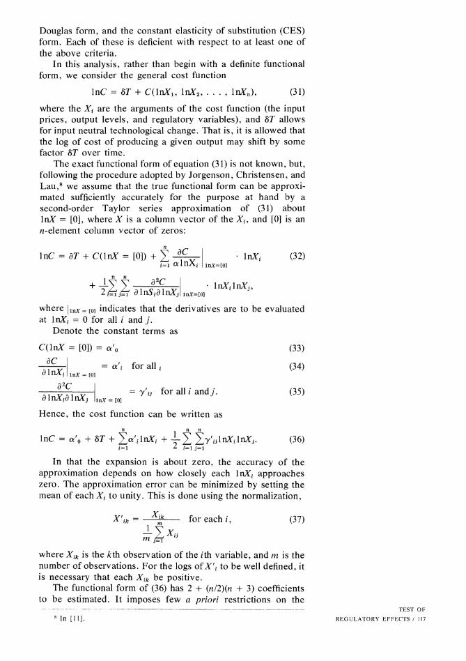
In this analysis, rather than begin with a definite functional form, we consider the general cost function

InC = aT + C(lnX1 , lnX2 , ••• , lnXn), (31)

where the X; are the arguments of the cost function (the input prices, output levels, and regulatory variables), and aT allows for input neutral technological change. That is, it is allowed that the log of cost of producing a given output may shift by some factor aT over time.

The exact functional form of equation (31) is not known, but, following the procedure adopted by Jorgenson, Christensen, and Lau,s we assume that the true functional form can be approxi­mated sufficiently accurately for the purpose at hand by a second-order Taylor series approximation of (31) about lnX = [0], where X is a column vector of the X;, and [0] is an n-element column vector of zeros:

InC = aT + C(lnX = [0)) + f ~I . lnX; (32) i=l aInX; 1nX=[0]

+ -L L a C . InX;lnXh 1 n n 2 I 2;=lj=1 aInS;alnXj 1nX=[0]

where 11nX = [0] indicates that the derivatives are to be evaluated at InX; = 0 for all i and j.

Denote the constant terms as

C(lnX = [0)) = a' 0

ac I ' for all ; alnX; 1nX = [0] = a i

a2

c I = y'ij for all i andj. a InXia InXj 1nX = [0]

Hence, the cost function can be written as

(33)

(34)

(35)

n 1 n n

InC = a'o + aT + La'iInX; + - L LY'ijlnX;lnXj . (36) ;=1 2 ;=1 j=l

In that the expansion is about zero, the accuracy of the approximation depends on how closely each lnX; approaches zero. The approximation error can be minimized by setting the mean of each Xi to unity. This is done using the normalization,

for each i, (37)

where X ik is the kth observation of the ith variable, and m is the number of observations. For the logs of X'i to be well defined, it is necessary that each X;k be positive.

The functional form of (36) has 2 + (n12)(n + 3) coefficients to be estimated. It imposes few a priori restrictions on the

" In [Ill. TEST OF

REG ULA TORY EFFECTS I 117

118 I H. CRAIG PETERSEN

parameters. Returns to scale cannot only be increasing, but can vary for different levels of output. The elasticity of substitution varies between inputs and for different levels of input usage. Technological change has been incorporated, and the model is easily estimable by simple linear methods. Thus, all of the re­quirements of functional form indicated by previous studies are satisfied. 9

In terms of the variables of Section 2, equation (36) becomes

InC' = ao + aT + Q{JInQ' + aLInP'L + aFInP'F + aKInP'K + aRIn«s - PK)') + 'YQQ(lnQ'F + 'YLL(lnP'L)2 + 'YKK(InP'K)2 + 'YFF(lnP'F)2 + 'YRR[ln«s - PK)')F + 'YQLInQ'lnP'L + 'YQFlnQ'lnP'F + 'YQKInQ'lnP'K + 'YQRInQ'In«s - PK)') + 'YLKInP'LInP'K + 'YLF InP'L InP'F + 'YLR InP'L In«s - PK)') + 'YKF InP'K InP'F + 'YKR InP'K In«s - PK)') + 'YFRlnP'Fln«s - PK)'), (38)

where the primes denote the normalized variables as given by equation (37), T is an index of technology, the Pi are input prices, Q is quantity, and s - PK is the difference between the allowed rate of return and the cost of capital, or "regulatory tightness." Equation (38) is the basic equation for determining the effect of regulation on unit costs.

N ext we consider the percentage of total expenditure going to capital. The estimating equation chosen is

PKKIC = bo + bQ InQ' + bQQ (lnQ')2 + bK InP'K + bFlnP'F + bLInP'L + bRln«s - PK)'). (39)

The theoretical model of Section 2 predicts that bR should be negative if an A-J effect is operative.

The statistical analysis is carried out using ordinary least squares (OLS). Behind the OLS methodology is the assumption that all variables on the right-hand side of equations (38) and (39) are either exogenous or predetermined. The presence of en­dogenous variables generates estimates of the coefficients which are biased. The Pi are exogenous as is s if the political influence of the firm on the commission is taken to be negligible. The quantity terms require some discussion. If there is no A-J effect, that is if the firm does not manipulate costs in the attempt to circumvent the regulatory constraint, then technology dictates costs and the price set by the commission is determined by technology and the allowed rate of return. Quantity as a function of price is, thus, exogenous to the firm. On the other hand, if tighter regulation results in higher costs, then the firm may be able to manipulate price and, hence, quantity. Note that as s decreases, costs increase. It is assumed that, if an A-J effect is operative, the two are offsetting, and the price fixed by the commission remains unchanged in equilibrium. Thus, quantity is exogenous to the firm. Such a result is a possible explanation for Stigler-Friedland's finding 10 that regulation had no effect on

9 The properties of functional forms such as (38) are discussed in Jorgenson, Christensen, and Lau [II].

10 In [18].

prices. In a related study!! the author has relaxed the assump­tion of quantity being exogenous and, using a simultaneous equation model and a different data set, tested for the A-J effect. The results are consistent with those of this analysis.

• The sample consists of fifty-six steam generating plants which experienced at least a fifty-percent expansion during the period 1960 to 1965. These are observed over the three-year period, 1966 to 1968. The selection of plants which significantly expanded capacity is dictated by the theoretical model which is derived in marginal terms. The analysis suggests that regulation causes planners to choose excessively capital-intensive produc­tion. Only in plants where capacity is being added is there much possibility for capital-other input substitution. Ex post substitu­tion in the industry is probably very limited.

The dependent variable used in estimation of (38) is the log of cost of production per unit of output in terms of dollars per thousand KWH. The dependent variable associated with (39) is the percent of total cost going to capital.

Output is in terms of millions of KWH of power. Fuel price is given as cost per million British Thermal Units of energy. The wage rate is expressed as dollars per year per employee. The capital price is formulated in terms of the annual rental price of capital as suggested by Jorgenson.!2 That is,

PK = q(r + 8 - q), (40)

where q is the price of equipment, r is the interest rate, 8 is the rate of depreciation, and q the rate of price change for equip­ment. An index of technology is constructed by determining the computed average time that capital had been in service. A dummy variable is included to distinguish plants which are owned by firms which are part of interstate holding companies. Participation in holding companies may be considered to be an additional scale variable.

Tightness of regulation proved difficult to quantify. Three measures are used in the analysis. First, as has been noted, four states during the study period did not have statewide regulatory commissions. Regulation is assumed to be less effective in these states. Thus, the model suggests that cost per unit of output should be lower in plants which operate in these states. Actual data consist of a dummy variable which takes on a value of one in states with commissions and zero in the states without com­missions.

Second, state commissions can be characterized as determin­ing the rate base on an original cost basis or on a fair value basis. The former method uses the value of the firm's capital as it appears on the firm's books, while the latter gives recognition to increased capital costs over time and may be five to fifty percent higher than original cost. Eiteman and Stuart!3 found that when the rate base was adjusted so as to be comparable in

II In [14]. 12 In [IOJ. I" In [8] and [19], respectively.

4. Data

TEST OF

REGULATORY EFFECTS I 119

120 / H. CRAIG PETERSEN

these two types of jurisdictions, a higher rate of return was, on average, allowed in fair value states. The differential was statis­tically significant. Thus, a second measure of "regulatory tight­ness" adopted is division of plants which operate in fair value states from those which operate in original cost jurisdictions. It is assumed that fair value regulation is more liberal in terms of allowed profits. The theoretical model predicts that average cost and percentage of cost going to capital should be lower in plants operating in these states. Data assume the form of a dummy variable taking on a value of one in states with original cost commissions and zero for states with fair value commissions or no state commission.

A third method of measuring regulatory stringency examines the return to equity capital. Because of the residual nature of the return to common stockholders, it is here that liberal or conser­vative commission policies are most dramatic. In a rate case an overall return on the capital base is allowed. Out of this total the firm must meet its debt, preferred stock, and common stock obligation; and its legal priorities are in that order. Fixed debt and preferred stock interest and dividends must be paid before common stockholders can receive dividends. Because of this legal priority, a one-percent change in the overall rate of return has a multiplied effect on the return to equity. If the firm has fifty-percent common stock in its capitalization, a one-percent change in the allowed rate of return has a two-percent effect on the return to equity. Thus, it is on the common stockholder that "tightness of regulation" is really felt.

The relationship between s - PK , the average allowed return minus the average cost of capital, and Se - Pe. the average return to equity minus the cost of equity, is just S - PK = (se - P e)(l - /3), where /3 is the percent of debt capital in the rate base. An index of Se - Pecan be derived based on the assumption that capital markets are efficient in their evalua­tion of a firm's relative profitability.

The value of a utility's stock at time 0 is given by the discounted value of the expected dividend stream,

MVo = IDt/(l + Pe)l, (41) 1=1

where MVo is the price of the firm's common stock at time 0, D t

is the dividend at time t and is given by the relationship Dt = DoO + g)f, where g is a constant rate of dividend growth.14

If the rate of dividend growth is less than the cost of capital, then (41) becomes

MVo = D 1/(Pe - g),

which can be solved for Pe:

P _ D1 e- MVo +g.

(42)

(43)

To return to equation (42), the dividend paid at time t is just the dividend pay-out ratio, d, times earnings per share for the

14 This model of stock price valuation is found in most introductory finance texts such as Van Horne [20).

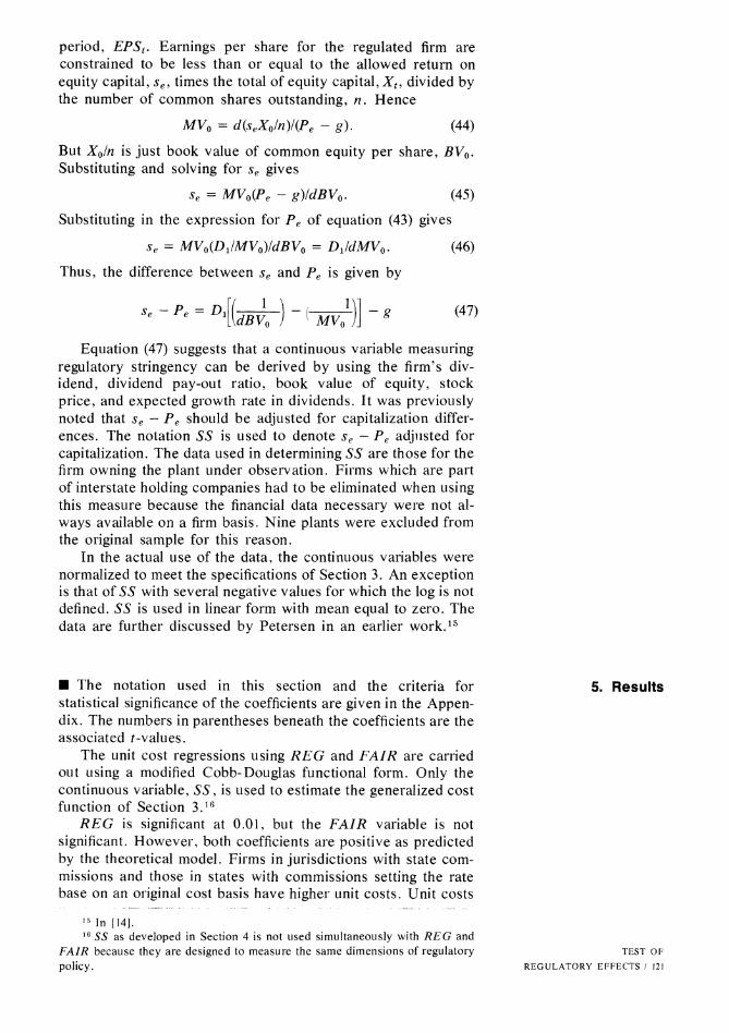
period, EPSt • Earnings per share for the regulated firm are constrained to be less than or equal to the allowed return on equity capital, Se' times the total of equity capital, Xt, divided by the number of common shares outstanding, n. Hence

MVo = d(seXo1n)/(Pe - g). (44)

But Xoln is just book value of common equity per share, BVo. Substituting and solving for Se gives

Se = MVo(Pe - g)ldBVo· (45)

Substituting in the expression for P e of equation (43) gives

Se = MVo(D!IMVo)ldBVo = D!ldMVo. (46)

Thus, the difference between Se and Pe is given by

(47)

Equation (47) suggests that a continuous variable measuring regulatory stringency can be derived by using the firm's div­idend, dividend pay-out ratio, book value of equity, stock price, and expected growth rate in dividends. It was previously noted that Se - P e should be adjusted for capitalization differ­ences. The notation S S is u sed to denote S e - P e adjnsted for capitalization. The data used in determining SS are those for the firm owning the plant under observation. Firms which are part of interstate holding companies had to be eliminated when using this measure because the financial data necessary were not al­ways available on a firm basis. Nine plants were excluded from the original sample for this reason.

In the actual use of the data, the continuous variables were normalized to meet the specifications of Section 3. An exception is that of SS with several negative values for which the log is not defined. SS is used in linear form with mean equal to zero. The data are further discussed by Petersen in an earlier work.!5

• The notation used in this section and the criteria for statistical significance of the coefficients are given in the Appen­dix. The numbers in parentheses beneath the coefficients are the associated t-values.

The unit cost regressions using REG and FAIR are carried out using a modified Cobb-Douglas functional form. Only the continuous variable, SS, is used to estimate the generalized cost function of Section 3. 16

REG is significant at 0.01, but the FAIR variable is not significant. However, both coefficients are positive as predicted by the theoretical model. Firms in jurisdictions with state com­missions and those in states with commissions setting the rate base on an original cost basis have higher unit costs. Unit costs

1.; In [14J. 16 SS as developed in Section 4 is not used simultaneously with REG and

FAIR because they are designed to measure the same dimensions of regulatory policy.

5. Results

TEST OF

REGULATORY EFFECTS I 121

122 I H. CRAIG PETERSEN

in states with commissions are, on average, seven percent higher.

Signs of other coefficients are consistent with a priori expec­tations. Fuel, labor, and capital price coefficients are all positive and significant. Newer vintage plants have significantly lower costs. The coefficients of the quantity variables imply that aver­age costs decrease with quantity out to a minimum of 4447 million KWH. Only seven plants in the sample exceeded that level of production.

Regression A

LCaST' = -0.1717 + 0.0880NH - 0.1008LQ' + 0.0590LQ'LQ' (3.85) (-8.11) (8.42)

+ 0.6237LF'+ 0.1784LL' + 0.2680LK' - 0.0189TC - 0.0006Y (15.26) (2.75) (2.18) (-4.45) (-0.06)

+ 0.0701REG + 0.0013FAIR (3.04) (0.08)

Number of observations: 168 R2 = 0.82.

Regression B uses the generalized cost function, but without the interaction terms of SS with LQ, LF, LL, and LK. The joint hypothesis that the coefficients of these terms are all zero can­not be rejected. The computed F-statistic is 0.759. The critical value at 0.05 is 2.45. The hypothesis that the appropriate func­tional form (when using SS) is a modified Cobb-Douglas, suoh as was used in Regression A, is, however, rejected.

The effect of changes in SS on the log of costs is given by:

dIne' = -3.627 - 550.2(SS'). dSS'

(48)

Equation (48) has a maximum at SS = -0.0066. In accor­dance with the requirements of Section 3, SS was normalized to have a mean equal to zero. In terms of the original data, the maximum occurs at SS' = 0.005. Less than fifteen percent of the observations on SS do not exceed that maximum point. The result suggests that the cost inflating effects of regulation can be reduced if the firm is regulated very tightly, but such an interpre­tation undoubtedly gives greater credit to the data and estima­tion procedures than their precision would justify. The estimates do suggest, however, that as regulation tightens, costs increase-although evidently at a decreasing rate.

For the other estimated coefficients of Regression B, all linear terms in input prices are positive and significant. Tech­nology results in a decrease in costs, and the unit cost curve decreases to a minimum at 7358 million KWH. This level is greater than for all but three of the output observations.

Regression B

LCaST' = -0.0185 -0.1160LQ' +0.0409LQ'LQ' -0.0127TC (-7.81) (4.19) (-3.20)

-0.OO20Y +0.5299LF' +0.3260LL' + 0.4088LK' -4.763LK'LK' (-0.23) (9.15) (4.79) (2.44) (- 3 .29)

+ 0.8516LF'LF' + 0.6055LL'LL' + 1.704LF'LK' -1.277LF'LL' (4.04) (1.36) (2.76) (-4.69)

+0.0846LF'LQ' -5.874LK'LL' +O.4lO2LK'LQ' +0.1943LL'LQ' (1.06) (-5.88) (2.00) (1.90)

- 3.625SS' (-3.73)

- 275.1SS'SS' ( -4.93)

Number of observations: 141 R2=0.87.

Turning to the percent of cost paid to capital, the basic estimating equation is (39). In actual practice, the Y and TC variables are included to allow for year-to-year and technology effects, and the NH variable to adjust for differences attribut­able to holding companies.

Using REG and FAIR, it is found that their coefficients are both positive and that of REG is significant at 0.01. Tighter regulation is associated with a greater proportion of cost going to capital. Looking at the other coefficients, both the linear and quadratic terms in quantity are significant. They suggest that there are savings on the use of capital in comparison to other inputs up to some point. The coefficient of the fuel price is negative and significant. The cost of fuel makes up a large component of total costs as found in the denominator of PC. The coefficient of the wage rate is positive and significant. This might be explained by substitution of capital for labor as wages increase, however previous studies such as that by Dhrymes and Kurz17 found little substitution between labor and capital. The capital price coefficient is negative but not significant. A possible explanation is that high rental rates on capital increase the cost of using a given amount of capital, but this is offset by substitution of other inputs (primarily fuel) as capital becomes more expensive. An interesting conclusion is that newer tech­nology in a plant seems to have no effect on the share of cost going to capital. This suggests that technology has been neutral among inputs or at least for capital as compared to labor and fuel considered together.

Regression C

PC = -0.0502 - 0.0114LQ' + 0.0132LQ'LQ' - 0.1510LF' (-2.40) (4.89) (-9.63)

+ 0.0675LL'- 0.0037LK' - .OO03TC - .0083Y (2.71) (-0.29) (-0.20) (-2.30)

+ 0.0223NH + .0267REG + .0026FAIR (2.53) (3.02) (0.38)

Number of observations: 168 R2 = 0.49.

When the continuous variable SS is used to determine the effect of regulation on the proportion paid to capital, the findings

17 In [7). TEST OF

REGULATORY EFFECTS / 123

6. Summary and conclusion

124 I H. CRAIG PETERSEN

are similar to those of Regression C. The signs of the quantity and input price variables are the same. Their magnitudes and t-statistics change quantitatively, but the comments made for Regression C still hold. SS is negative and significant at 0.01. As regulation becomes more stringent, the firm spends a greater fraction of total cost on capital.

Regression D

PC = -0.0036 - 0.0095LQ' + 0.0132LQ'LQ' - 0.1878LF' (-1.80) (4.62) (-9.09)

+ 0.1023LL' - 0.0253LK' + 0.0013TC - 0.0090Y - 1.336SS' (3.53) (-0.41) (0.70) (-2.20) (-2.96)

Number of observations: 141 R2 = 0.50 .

• The Averch-lohnson model provides analytical support for the proposition that rate of return regulation may result in inefficient production. In this paper the A-l model is reformu­lated in terms of cost-minimization subject to the regulatory constraint. It is shown that as regulation tightens, that is, as the allowed return approaches the cost of capital, the firm has higher unit costs and spends a larger portion of total cost on capital. These two relationships are testable hypotheses of the revised A-l model.

A general functional form is adopted for empirical analysis. This form does not put a priori restrictions on the coefficients of the cost function. The sample consists of steam generating plants which experience a large addition to capacity just prior to the sample period, 1966 to 1968. Three measures of regulatory policy with regard to the allowed return are used. The first is the dichotomy between firms operating in states with state commis­sions and those without. The second is the separation of original cost from fair value rate base jurisdictions. It is assumed that regulation is more strict in states with state commissions and in original cost jurisdictions. The third measure is an attempt to measure the actual difference between the allowed return and the cost of capital.

The evidence supports the hypotheses. Using both a modified Cobb- Douglas and the more general form of the cost function, it is found that as regulation tightens, unit costs in­crease. The result is statistically significant using the state com­mission versus no state commission dichotomy and also using the continuous measure of the allowed return minus the cdst of capital. It is also found that the percent of cost going to capital increases with more stringent regulation. This result is also statistically significant when the same two measures are used.

In summary, the findings of this analysis are that the empiri­cal evidence does support the Averch-lohnson contention. The conclusions here are also generally consistent with those previ­ously reported by Spann and by Courville. Additional results on

this topic and on other effects of regulation are presented in an earlier work of the author. 18

Appendix

• The following notation is used in reporting the results of the econometric analysis:

LcaST PC Y TC LQ LL LK LF REG

FAIR

SS

NH

LQLQ LQLL LQLF LQLK

Log of unit cost of production. Percent of total unit cost going to capital. Year of observation. Index of technological change. Log of quantity produced. Log of annual wage rate. Log of capital rental rate. Log of fuel price. Dummy variable. Value equals one for firms under staie commission. Dummy variable. Value equals one for firms regu­lated on an original cost basis. Allowed return on equity minus the cost of equity capital adjusted for capitalization differences. Dummy variable. Value equals one if firm is part of a holding company. Log of quantity times log of quantity. Log of quantity times log of wage rate. Log of quantity times log of fuel price. Log of quantity times log of capital rental rate.

In general, products of two variables required by equation (38) are denoted by LiLj where Li and Lj are the respective variable names. The last four entrys in the column above are examples.

Standard tests of statistical significance are used. In most cases a coefficient will be considered significantly different from zero if it passes a two-tailed (-test at an alpha level of 0.05. If the sign of the coefficient is given by the theoretical model or a priori expectation, then a one-tail test at 0.05 will be the criteria.

References

l. AVERCH. H. AND JOHNSON. L. L. "'Behavior of the Firm under Regulatory Constraint." The American Economic Review, Vol. 52. No.5 (December 1962), pp, 1053-1069.

2. BAILEY, E. Economic Theory of Regulatory Constraint. Lexington, Mass.: D.C. Heath, 1973.

3. BARZEL, Y. "The Production Function and Technological Change in the Steam Power Industry." Journal of Political Economy, Vol. 72, No.2 (April 1964), pp. 133-150.

4. BAUMOL, W. AND KLEVORICK, A. "Input Choices and Rate of Return Regulation: An Overview of the Discussion." The Bell Journal of Economics and Management Science, Vol. I, No.2 (Autumn 1970), pp. 162-190.

'" In [14]. TEST OF

REGULATORY EFFECTS I 125

126 I H. CRAIG PETERSEN

5. CLARK, DODGE, AND COMPANY. An Outline of Electric Utility Regulation by States. New York, 1962.

6. COURVILLE, L. "Regulation and Efficiency in the Electric Utility Industry." The Bell Journal of Economics and Management Science, Vol. 5, No. I (Spring 1974). pp. 53-74.

7. DHRYMES, P. J. AND KURZ, M. "Technology and Scale in Electricity Gen­eration." Econometrica, Vol. 32, No.4 (July 1964), pp. 287-315.

8. EITEMAN, D. K. "Interdependence of Utility Rate-Base Type, Permitted Rate of Return, and Utility Earnings." Journal of Finance, Vol. 17, No.1 (March 1962), pp. 38-52.

9. FEDERAL POWER COMMISSION. Federal and State Commission Jurisdiction and Regulation. Washington, D.C.: U.S. Government Printing Office.

10. JORGENSON, D. W. "Capital Theory and Investment Behavior." The Ameri­can Economic Review. Vol. 53, No.2 (May 1963), pp. 247-259.

11. ---, CHRISTENSEN, L. R., AND LAU, L. J. "Conjugate Duality and the Transcendental Logarithmic Function." Stanford University Working Pa­per, 1971.

12. NERLOVE, M. "Returns to Scale in Electricity Supply," in C. Christ et al., Measurement in Economics. Stanford: Stanford Univ. Press, 1963, pp. 167-198.

13. PETERSON, H. C. "The Allowed Rate of Return vs. the Marginal Cost of Captial in a Public Utility Rate Case." #74-2, Center Study Papers, Economics Research Center, Utah State University, January, 1974.

14. ---. 'The Effect of Regulation on Production Costs and Output Prices in the Private Electric Utility Industry." Memorandum No. /5/, Stanford University Center for Research in Economic Growth, Stanford University, September, 1973.

15. PHILLIPS, C. F., JR. The Economics of Regulation. Homewood, Ill.: R. D. Irwin, Inc., 1969.

16. RESCHENTHALER, G. B. "The Legal Background of Electric Utility Regula­tion in Texas-An Economist's View." Baylor Law Review, Vol. 21, No.3 (Summer 1969). pp. 295-304.

17. SPANN, R. M. "Rate of Return Regulation and Efficiency in Production: An Empirical Test of the Averch-Johnson Thesis." The Bell Journal of Economics and Management Science, Vol. 5, No. 1 (Spring 1974), pp. 38-52.

18. STIGLER, G. AND FRIEDLAND, C. "What Can the Regulators Regulate: The Case of Electricity." Journal of Law and Economics. Vol. 5 (October 1962), pp. 1-16.

19. STUART, F. "Rate Base versus Rate of Return." Public Utilities Fort­nightly, Vol. 70 (September 21, 1962), pp. 395-99.

20. VAN HORNE, J. C. Financial Management and Policy. Englewood Cliffs, N.J.: Prentice-Hall, Inc., 1971.