An Empirical Study on Progressive Sampling forJust-in-Time Software Defect Prediction

Xingguang Yang∗†, Huiqun Yu∗‡�, Guisheng Fan∗�, Kang Yang∗, Kai Shi§∗Department of Computer Science and Engineering, East China University of Science and Technology, Shanghai 200237, China

†Shanghai Key Laboratory of Computer Software Evaluating and Testing, Shanghai 201112, China‡Shanghai Engineering Research Center of Smart Energy, Shanghai, China

§Alibaba Group, Hangzhou, China

Abstract—Just-in-time software defect prediction (JIT-SDP) isan active research topic in the field of software engineering,aiming at identifying defect-inducing code changes. Most existingJIT-SDP work focuses on improving the prediction performanceof the model by improving the model. However, a frequentlyignored problem is that collecting large and high quality defectdata sets is costly. Specifically, when labelling the samples, expertsin the field are required to carefully analyze the defect reportinformation and log of code modification, which requires a lotof effort. Therefore, how to build a high-performance JIT-SDPmodel with a small number of training samples is an issue worthstudying, which can reduce the size of the defect data sets andreduce the cost of data sets acquisition. This work thus providesa first investigation of the problem by introducing a progressivesampling method. Progressive sampling is a sampling strategythat determines the minimum number of training samples whileguaranteeing the performance of the model. However, progressivesampling requires that the learning curve of the prediction modelbe well behaved. Thus, we validate the availability of progressivesampling in the JIT-SDP issue based on six open-source projectswith 227417 changes. Experimental results demonstrate thatthe learning curve of the prediction model is well behaved.Therefore, the progressive sampling is feasible to tackle the JIT-SDP problem. Further, we investigate the optimal training samplesize derived by progressive sampling for six projects. Empiricalresults demonstrate that a high-performance prediction modelcan be built using only a small number of training samples. Thus,we recommend adopting progressive sampling to determine thesize of training samples for the JIT-SDP problem.

Index Terms—Just-in-time, software defect prediction, progres-sive sampling, mining software repositories

I. INTRODUCTION

Defects in the software system can cause huge losses tocompanies [1]. Although software quality activities (such assource code checking and unit testing) can reduce the numberof defects in software, they require a lot of testing resources.Therefore, how to release a high-quality software projectwith limited testing resources is a huge challenge in thefield of software engineering [2]. Software defect predictionis an effective method. Developers use machine learning orstatistical learning methods to identify the defect-proneness ofprogram modules in advance, thereby investing more limitedtesting resources into defect-prone modules [2].

Corresponding Authors: Huiqun Yu (yhq@ecust.edu.cn), Guisheng Fan(gsfan@ecust.edu.cn)

Just-in-time software defect prediction(JIT-SDP) is a morefine-grained defect prediction method, which is made atchange-level rather than module-level(e.g., function, file, andclass) [1]. In the software development process, once the de-veloper submits a modification to the software code, the defectprediction model will predict the defect-proneness of the code.If the change is predicted to be buggy, the correspondingdeveloper will be assigned to check the change. Therefore,JIT-SDP has the advantages of fine granularity, instantaneity,and traceability [3], and has been adopted by many companiessuch as Lucent [4], BlackBerry [5], Cisco [6], etc.

Recently, JIT-SDP has received extensive attention andresearch. The main research work focuses on model building[7] [8], feature selection [1] [9], data annotation [10], etc.However, few studies have focused on the cost of acquiringdefect data sets. Specifically, in order to obtain high-qualitydefect data sets, experts in specific fields are required to ana-lyze version control systems (SVN, CVS, Git, etc.) and defecttracking systems (Bugzlla or Jira) during the data annotationphase [3]. Therefore, constructing an accurate defect dataset is costly [11]. In the field of software engineering datamining [12] [13], researchers found the following relationshipbetween the size of the data sets and the performance of theprediction model: When the data set size is small, the accuracyof the prediction model increases significantly as the size ofthe data increases. When the data sets size exceeds a certainnumber, adding more data does not lead to higher predictionperformance. Therefore, how to build a high performanceprediction model with fewer training samples for JIT-SDP isa problem worth studying, which brings two advantages:

• Firstly, reducing the size of training samples can reducethe cost of data sets labeling.

• Secondly, when using complex learning algorithms suchas deep learning algorithms [8], reducing the size of thetraining data can significantly reduce the time requiredfor model training.

In order to reduce the use of training samples, this paperfirst introduces progressive sampling into the study of JIT-SDPproblems. We conduct experiment on the change-level defectdata sets from six open source projects with 227417 changes.The main contributions of this paper are as follows:

7th International Workshop on Quantitative Approaches to Software Quality (QuASoQ 2019)

Copyright © 2019 for this paper by its authors. Use permitted under Creative Commons License Attribution 4.0 International (CC BY 4.0).

12

• We introduce progressive sampling to the JIT-SDP studyto determine the optimal training sample size and reducethe cost of defect data acquisition. However, progres-sive sampling requires that the learning curve of theprediction model be well behaved in coarse granularity.Therefore we conduct a large-scale empirical study basedon the defect data sets from six open-source projects.The experimental results show that the learning curveof the prediction model is well behaved. So progressivesampling is efficient for JIT-SDP.

• We further investigate the optimal training sample sizederived by progressive sampling based on six open-source projects. The experiment uses the random forestto establish a prediction model and uses AUC to evaluatethe performance of the model. Empirical results showthat using progressive sampling can significantly reducethe number of training samples used while guaranteeingthe performance of the prediction model. Therefore, werecommend that in the practical application of JIT-SDP,using progressive sampling can effectively reduce theamount of training samples and reduce the cost of modelbuilding.

The rest of the paper is organized as follows: The relatedwork is described in Section II. Section III introduces theprogressive sampling and it’s application in the scenario ofJIT-SDP. Experimental setup is described in the Section IV.Section V introduces the experimental results and discussion.Section VI introduces the threats to validity. Conclusions andfuture work is described in the Section VII.

II. RELATED WORK

A. Just-in-Time Software Defect Prediction

JIT-SDP is a special method for predicting software defects.Unlike traditional defect prediction, JIT-SDP is performed atchange-level, which has finer granularity. Mockus and Weiss[4] first proposed the idea of JIT-SDP, and they designed anumber of change metrics to predict whether changes aredefect-inducing or clean. Recently, Kamei et al. [1] performeda large-scale empirical study in JIT-SDP. They collected elevendata sets from six open-source projects and five commercialprojects. Their experimental results show that their predictionmodel can achieve 68% accuracy and 64% recall. Moreover,they find that 35% defect-inducing changes can be identifiedusing only 20% of the effort.

Subsequently, researchers proposed various methods to im-prove the performance of the prediction model for JIT-SDP.Chen et al. [14] designed two objects through the benefit-costanalysis, and formalized the JIT-SDP problem into a multi-objective optimization problem. They proposed a methodcalled MULTI based on NSGA-II [15]. The experimentalresults show that MULTI can significantly improve the effort-aware prediction performance for JIT-SDP. Furthermore, Yanget al. [16] found that the MULTI method is more biasedtowards the benefit object in the optimal solution selection.Therefore, they proposed a benefit-priority optimal solution

selection strategy to improve the performance of the MULTImethod. Cabral et al. [17] first found that JIT-SDP suffers fromclass imbalance evolution. Their proposed approach can obtaintop-ranked g-means compared with state-of-the-art methods.

B. Progressive Sampling

Weiss and Tian pointed out that in the field of data mining,data acquisition is one of the main costs of the process ofbuilding a classification model [18]. Therefore, reducing theuse of training data while guaranteeing the performance ofthe prediction model can reduce the cost of model building.In solving the actual classification task, using fewer trainingsamples can still get a high prediction model. Thus, Provostet al. [19] proposed progressive sampling method. Progressivesampling continuously increases the number of training sam-ples by the iterative method. Currently progressive samplinghas been widely used in the field of software engineering datamining. For example, in the study of performance predictionfor configurable software, obtaining data sets is costly. Thus,Sarkar et al. [12] used progressive sampling to determine theoptimal number of training samples.

In the JIT-SDP study, obtaining high-quality defect datasets is costly, and it requires specialists in specific fieldsto thoroughly analyze defect report information and codemodification logs [11]. The most existing JIT-SDP study onlyfocuses on improving the performance of the prediction model,but ignores the cost of defect data sets acquisition. Therefore,this paper first introduces progressive sampling into the JIT-SDP scenario.

III. PROGRESSIVE SAMPLING

A. Basic Concept of Progressive Sampling

Progressive sampling is a popular sampling strategy thathas been used for various learning models [13]. Progressivesampling is an iterative process whose basic idea is to generatean array of integers n0, n1, n2, ..., nk. Each integer ni indicatesthat the training samples with size of ni are used to buildthe prediction model at the ith iteration. According to thecalculation of the number of training samples in each iteration,progressive sampling can be classified as arithmetic progres-sive sampling and geometric progressive sampling [20]. Thesize of training samples for two progressive sampling iscalculated as shown in Eq. (1) and Eq. (2), respectively, wheren0 represents the initial training sample size and a determinesthe growth rate of the training samples. It can be seen thatthe main difference between the two kinds of progressivesampling is that the geometric progressive sampling has alarger growth rate than the arithmetic progressive sampling,and is suitable for the prediction model with high algorithmcomplexity. Since the machine learning algorithm used in thispaper is the random forest [21], the training time of the modelis short, so it is suitable to use arithmetic progressive sampling.

ni = n0 + i ∗ a (1)

ni = n0 ∗ ai (2)

7th International Workshop on Quantitative Approaches to Software Quality (QuASoQ 2019)

Copyright © 2019 for this paper by its authors. Use permitted under Creative Commons License Attribution 4.0 International (CC BY 4.0).

13

Learning curve. The learning curve [19] describes theprediction performance of the prediction model at differenttraining sample sizes and can clearly characterize the learningprocess of progressive sampling. Typical learning curve isshown as Fig.1, where the x-axis represents the training samplesize and the y-axis represents the prediction performance ofthe model. A well behaved learning curve is monotonicallynon-decreasing and contains three regions: In the first region,the model performance increases rapidly as the training samplesize increases; in the second region, the model performanceincreases slowly as the training sample size increases; in thethird region, adding more training samples will not signifi-cantly improve the performance of the model.

Training sample size

Perfo

rman

ce

Fig. 1. Learning Curve

B. The Process of Progressive Sampling in the JIT-SDPProgressive sampling is widely used in various software

engineering related studies, such as performance prediction ofconfigurable software [12], etc. In this paper, we first introduceprogressive sampling into the JIT-SDP scenario. The detailedprocess is shown in Fig. 2, which involves four steps asfollowing:

Start

Developers Software history

repositoryData sets

Prediction

modelAcceptable?

Increase training

samples

End

Y

N

Fig. 2. The process of progressive sampling in the JIT-SDP

1) Developers mine metrics related to software changes fromthe software history repositories.

2) Domain experts label samples as defect-inducing or cleanby analyzing defect reporting information and code mod-ification logs in version control systems, and build defect

data sets. Because of the high cost of this process, onlya few number of changes are labeled.

3) Based on the existing data sets, a machine learningalgorithm is used to build a defect prediction model.

4) After the prediction model is evaluated, it is requiredto determine whether the performance of the model isacceptable. If the performance is not acceptable, the moretraining samples will be collected according to the rulesof progressive sampling.

We use following Algorithm 1 to describe more formallythe application process of progressive sampling in JIT-SDP.

Algorithm 1: The progressive sampling for JIT-SDPInput: initial sample size: n0; growth factor: a;

termination threshold: threshold AUCOutput: prediction model: model;

1 begin2 # Build data sets with n0 samples3 D = mining software repository(n0)4 while true do5 # Split data sets into training and test sets6 train set, test set = train test split(D)7 # Build prediction model based on machine

learning methods8 model = Random Forest(train set)9 # Model evaluation

10 AUC = Evaluation(model, test set)11 # Whether the model is acceptable12 if AUC > threshold AUC then13 return model14 end15 else16 new D =

mining software repository(a)17 D = D ∪ new D18 end19 end20 end

We denote an instance of a code change as X ={x1, x2, ..., xm}, where x1, x2, ..., xm represent the m metricsof the change X . An example of the change X is denotedas (x, Y ), where x represents the values of metrics and Yrepresents whether the change is buggy or clean. If the changeX is identified as buggy, then Y will be marked as 1, otherwiseit is marked as 0. The defect data sets D for a specific projectare composed of a set of examples X , where X ⊆ D.

In the beginning, developers need to mine n0 samples fromthe software history repositories and build data sets D (Line3). The data sets are then split into training and test sets (Line6). The the defect prediction model is built and evaluatedbased on a machine learning algorithm (Line 8-10). Ourexperiment uses the random forest to build a prediction modeland evaluate the model using AUC. If the performance of themodel exceeds the threshold threshold AUC, the progressive

7th International Workshop on Quantitative Approaches to Software Quality (QuASoQ 2019)

Copyright © 2019 for this paper by its authors. Use permitted under Creative Commons License Attribution 4.0 International (CC BY 4.0).

14

sampling terminates the iteration (Line 12-13). Otherwise, itis necessary to further collect a samples from the softwarehistory repositories to increase the size of the data sets (Line16-17).

IV. EXPERIMENTAL SETUP

This paper introduces progressive sampling into the JIT-SDPproblem and designs the following two research questions:

• RQ1: Whether the progressive sampling is feasible in theJIT-SDP scenario?

• RQ2: What is the optimal training sample size to estab-lish a high performance prediction model by adoptingprogressive sampling?

The experimental hardware environment is Intel(R)Core(TM)I7-7700 CPU RAM: 8G. The programming environ-ment used in the experiment is python3.2.

A. Data Sets

The data sets used in the experiment were provided byKamei et al. [1] and are widely used in the field of JIT-SDP [7] [8] [9]. The data sets are collected from sixopen source projects, namely Bugzilla(BUG), Columba(COL),Eclipse JDT(JDT), Eclipse Platform(PLA), Mozilla(MOZ), andPostgreSQL(POS), with a total of 227417 changes. The num-ber of defective changes, defect rate, and data collection periodfor each subject system are shown in Table I.

TABLE ITHE BASIC INFORMATION OF DATA SETS

Project Period #defectivechanges #changes %defect

rate

BUG 1998/08/26∼2006/12/16 1696 4620 36.71%COL 2002/11/25∼2006/07/27 1361 4455 30.55%JDT 2001/05/02∼2007/12/31 5089 35386 14.38%MOZ 2000/01/01∼2006/12/17 5149 98275 5.24%PLA 2001/05/02∼2007/12/31 9452 64250 14.71%POS 1996/07/09∼2010/05/15 5119 20431 25.06%

In order to accurately predict defects for software changes,Kamei et al. [1] designed 14 metrics. These metrics can bedivided into five dimensions: diffusion, size, purpose, history,and experience. The specific description information is shownin Table II.

B. Prediction Model

Similar to previous research [22], the experiment uses therandom forest algorithm to build prediction models [21],because previous studies have shown that random forest ishighly robust, accurate and stable on JIT-SDP issues [23], andexceed other modeling techniques [24].

Random forest is an ensemble learning algorithm based ondecision tree. Different from the conventional decision tree,the base learner randomly selects a subset of the attributes ineach node’s attribute set, and then selects an optimal attributefrom the subset. Random forest algorithm is simple, easy toimplement, and has low computational overhead, and is widelyused in various learning tasks.

TABLE IITHE DESCRIPTION OF METRICS

Dimension Metric Description

Diffusion

NS Number of modified subsystemsND Number of modified directoriesNF Number of modified filesEntropy Distribution of modified code across each file

SizeLA Lines of code addedLD Lines of code deletedLT Lines of code in a file before the change

Purpose FIX Whether or not the change is a defect fix

HistoryNDEV Number of developers that changed the files

AGE Average time interval between the lastand the current change

NUC Number of unique last changes to the files

ExperienceEXP Developer experienceREXP Recent developer experienceSEXP Developer experience on a subsystem

C. Performance Indicators

The test samples can be divided into true positive(TP),false negative(FN), false positive(FP), and true negative(TN)according to the labels of the samples and the predictionresults. The confusion matrix of the classification results isshown in the Table III. JIT-SDP is a binary classificationproblem. Common evaluation indicators include precision,recall, accuracy, etc. However, since the defect data sets areusually class-imbalanced, these threshold-based evaluation in-dicators are sensitive to threshold settings. Therefore, thresholdindependent evaluation indicators should be used [25].

The experiment uses AUC to evaluate the prediction per-formance of the model [1] [22]. AUC (Area Under Curve)is the area under the ROC curve. The ROC (Receiver Op-erating Characteristic) curve is drawn as follows: First, thetest examples are sorted in descending order according tothe probability that the prediction is positive; then the testexamples are regarded as positive classes one by one, andthe true positive rate (TPR) and false positive rate (FPR) arecalculated each time; using TPR as the ordinate and FPR asthe abscissa, one point of the ROC curve is obtained, and thesepoints are connected to obtain the ROC curve.

TPR =TP

TP + FN(3)

FPR =FP

TN + FP(4)

TABLE IIICONFUSION MATRIX

Actual value Prediction resultPositive Negative

Positive TP FNNegative FP TN

D. Data Preprocessing

In order to improve the prediction performance of themodel, according to the recommendations of Kamei et al. [1],we conduct the following preprocessing on the data sets:

7th International Workshop on Quantitative Approaches to Software Quality (QuASoQ 2019)

Copyright © 2019 for this paper by its authors. Use permitted under Creative Commons License Attribution 4.0 International (CC BY 4.0).

15

1) Remove highly correlated metrics. Since NF and ND,REXP and EXP are highly correlated, ND and REXPare excluded. Since LA and LD are highly correlated,LA and LD are normalized by dividing by LT. Since LTand NUC are highly correlated with NF, LT and NUCare normalized by dividing by NF.

2) Logarithmic transformation. Since most metrics arehighly skewed, each metric(except for fix) performs alogarithmic transformation.

3) Dealing with class imbalance. The data sets used inthe experiment are class-imbalanced, i.e., the number ofdefect-inducing changes is far more than the number ofclean changes. Therefore, we perform random undersam-pling on the training set. By randomly removing the cleanchanges, the number of defect-inducing changes is thesame as the number of clean changes.

V. EXPERIMENTAL RESULTS AND DISCUSSION

This section answers the questions raised in Section IVthrough experiments.

A. Analysis for RQ1

Motivation. Progressive sampling is an effective means ofdetermining the optimal training sample size, and is widelyused in the field of software engineering [12]. This paper firstintroduces progressive sampling into the JIT-SDP problem todetermine the optimal training sample size for the predic-tion model. However, in practical applications, progressivesampling requires that the learning curve of the predictionmodel be well behaved [19]. The basic characteristic of awell behaved learning curve is that the slope of the learningcurve is monotonically non-increasing at the level of coarsegranularity [19]. Therefore, we aim to verify whether progres-sive sampling is feasible on JIT-SDP issues through empiricalresearch.

Approach. The experiment uses the six open source projectsintroduced in the Section IV as the research object to explorewhether the learning curve of the JIT-SDP model is wellbehaved. Because the prediction model is based on a fasttraining random forest algorithm, the arithmetic progressivesampling method is adopted. To plot a learning curve for eachdata sets, we divided the data sets into two parts: 50% as thetraining pool for the constructing training sets and 50% as thetest sets for the model evaluation. The two parameters of thearithmetic progressive sampling are as follows:

• n0 = |training pool| ∗ 1%• a = |training pool| ∗ 1%

Since progressive sampling requires the learning curve tobe well behaved in coarse grain size, the granularity of ourparameter settings is large. The initial number of trainingsamples is 1% of the total number of training pools, and 1%of the number of training samples is added per iteration.

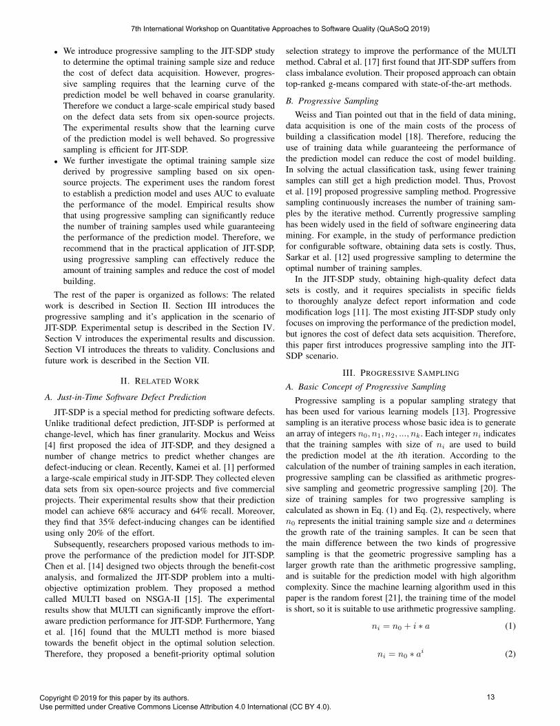
Findings. The experimental results are shown in Fig. 3,which contains six subgraphs, each of which represents a

learning curve for a project, where the horizontal axis rep-resents the size of training samples and the vertical axisrepresents the performance of the prediction model.

As can be seen from Fig. 3, the learning curve for eachsystem is well behaved, which is generally monotonicallynon-decreasing. Although the learning curve fluctuates inlocal areas, the general trend is monotonically non-decreasing.Therefore, we can draw a conclusion that progressive samplingis feasible in the JIT-SDP problem.

B. Analysis for RQ2

Motivation. The Section V-A has proven that progressivesampling is feasible in the JIT-SDP problem. However, whatis the optimal training sample size to establish a high perfor-mance prediction model by adopting progressive sampling isa question worth studying. If a high-performance predictionmodel can be built with very few training samples, then onlya small number of data sets need to be labelled during theconstruction of the defect data sets, which can greatly reducethe cost of data sets acquisition. Therefore, it is necessary tofurther investigate the optimal training sample size based onprogressive sampling for JIT-SDP.

Approach. The experiment uses the data sets of the sixprojects introduced in Section IV. The prediction model isbuilt based on the random forest, and the optimal trainingsample size is calculated based on the arithmetic progressivesampling. The experimental data sets are divided into twoparts: 50% as a training pool for generating training sets and50% as test sets for model evaluation. The parameters of thearithmetic progressive sampling are as follows: First, the initialsample size should be set small, so n0 is set to 0.5% of thesize of training pool. Second, since the training time of themodel is short, the number of samples added at each iterationshould not be too large. The experiment sets the growth ratea to 20. The threshold in the progressive sampling is used todetermine whether the performance of the model is acceptable.Threshold settings are usually given by experts in a particularfield. Previous studies have shown that the AUC value of theJIT-SDP model is usually not lower than 0.75 [22]. Therefore,the threshold of acceptable performance threshold AUC isset to 0.75, i.e., once the AUC value of the prediction modelis greater than or equal to 0.75, the progressive samplingterminates the iteration and returns the value of training samplesize.

• n0 = |training pool| ∗ 0.5%• a = 20• threshold AUC = 0.75

For better generalizability of experimental results, and tocounter random observation bias, the entire experiment isrepeated 100 times.

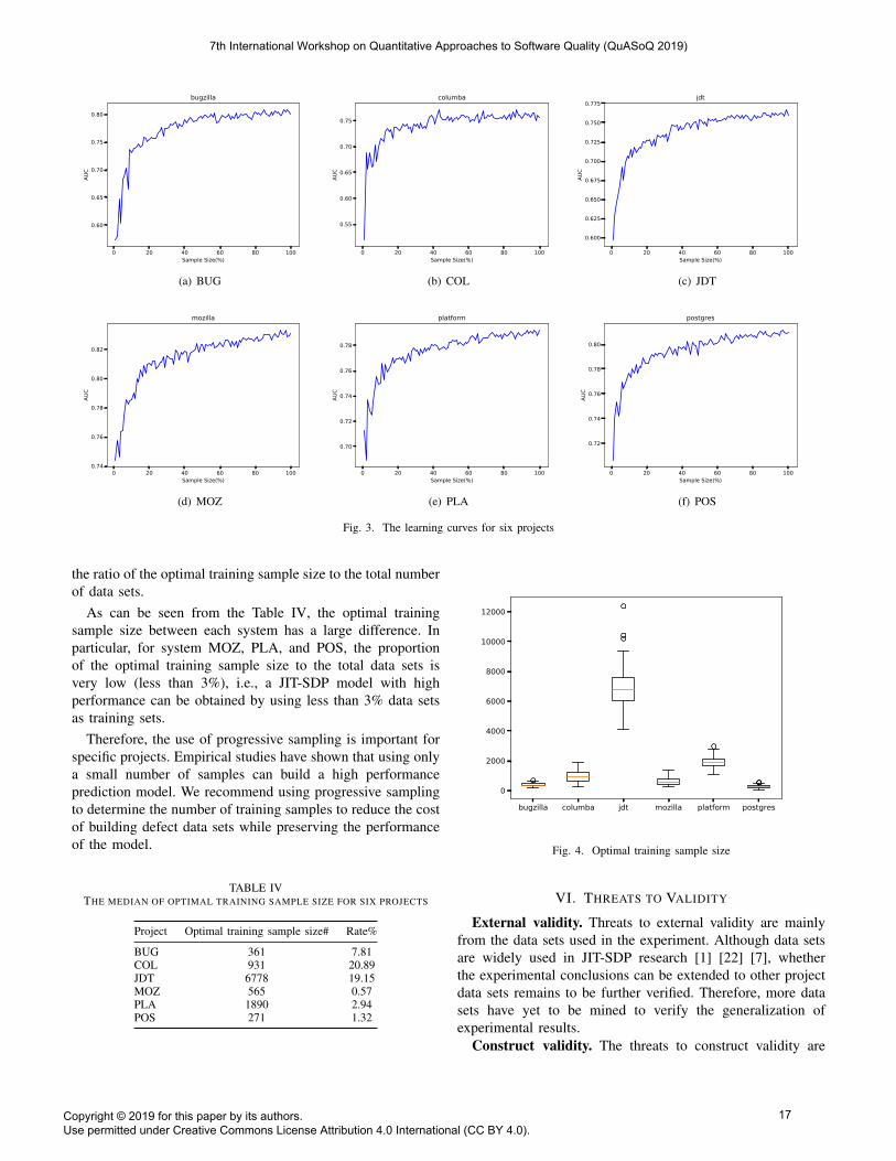
Findings. The experimental results are shown in Fig. 4,which describes box plots of optimal training sample sizes forsix projects. Table IV shows the median of optimal trainingsample size for six projects, where the second column repre-sents the median of optimal training sample sizes calculatedfrom 100 experimental results, and the third column represents

7th International Workshop on Quantitative Approaches to Software Quality (QuASoQ 2019)

Copyright © 2019 for this paper by its authors. Use permitted under Creative Commons License Attribution 4.0 International (CC BY 4.0).

16

0 20 40 60 80 100Sample Size(%)

0.60

0.65

0.70

0.75

0.80

AUC

bugzilla

(a) BUG

0 20 40 60 80 100Sample Size(%)

0.55

0.60

0.65

0.70

0.75

AUC

columba

(b) COL

0 20 40 60 80 100Sample Size(%)

0.600

0.625

0.650

0.675

0.700

0.725

0.750

0.775

AUC

jdt

(c) JDT

0 20 40 60 80 100Sample Size(%)

0.74

0.76

0.78

0.80

0.82

AUC

mozilla

(d) MOZ

0 20 40 60 80 100Sample Size(%)

0.70

0.72

0.74

0.76

0.78AU

C

platform

(e) PLA

0 20 40 60 80 100Sample Size(%)

0.72

0.74

0.76

0.78

0.80

AUC

postgres

(f) POS

Fig. 3. The learning curves for six projects

the ratio of the optimal training sample size to the total numberof data sets.

As can be seen from the Table IV, the optimal trainingsample size between each system has a large difference. Inparticular, for system MOZ, PLA, and POS, the proportionof the optimal training sample size to the total data sets isvery low (less than 3%), i.e., a JIT-SDP model with highperformance can be obtained by using less than 3% data setsas training sets.

Therefore, the use of progressive sampling is important forspecific projects. Empirical studies have shown that using onlya small number of samples can build a high performanceprediction model. We recommend using progressive samplingto determine the number of training samples to reduce the costof building defect data sets while preserving the performanceof the model.

TABLE IVTHE MEDIAN OF OPTIMAL TRAINING SAMPLE SIZE FOR SIX PROJECTS

Project Optimal training sample size# Rate%

BUG 361 7.81COL 931 20.89JDT 6778 19.15MOZ 565 0.57PLA 1890 2.94POS 271 1.32

bugzilla columba jdt mozilla platform postgres

0

2000

4000

6000

8000

10000

12000

Fig. 4. Optimal training sample size

VI. THREATS TO VALIDITY

External validity. Threats to external validity are mainlyfrom the data sets used in the experiment. Although data setsare widely used in JIT-SDP research [1] [22] [7], whetherthe experimental conclusions can be extended to other projectdata sets remains to be further verified. Therefore, more datasets have yet to be mined to verify the generalization ofexperimental results.

Construct validity. The threats to construct validity are

7th International Workshop on Quantitative Approaches to Software Quality (QuASoQ 2019)

Copyright © 2019 for this paper by its authors. Use permitted under Creative Commons License Attribution 4.0 International (CC BY 4.0).

17

mainly considered whether the evaluation indicator used in ourexperiment can accurately reflect the prediction performanceof the prediction model. The experiment uses AUC to evaluatethe JIT-SDP model, which is also widely adopted by previousresearch [22].

Internal validity. The threats to internal validity are mainlyfrom experimental code. Our experimental code is written inpython. In order to reduce errors in the code, we used maturelibraries and carefully checked the code of the experiment.

VII. CONCLUSIONS AND FUTURE WORK

In this paper, we first introduce progressive sampling for theJIT-SDP. Progressive sampling is a commonly used samplingstrategy that progressively increases the number of trainingsamples to determine the optimal number of training sam-ples.The experiment is conducted on six open source projectswith 227417 changes. Our prediction model is built based onthe random forest algorithm and evaluated by AUC.

Large-scale empirical studies demonstrate that progressivesampling is feasible in the JIT-SDP scenario. Moreover, ex-perimental results show that the optimal training sample sizederived by progressive sampling is very small. Especially, theproportion of training samples to the total number of datasets is less than 3% on the projects MOZ, PLA, and POS.Therefore, we suggest that progressive sampling can be used inthe practical application of JIT-SDP to determine the optimalnumber of samples, thereby reducing the number of trainingsamples and reducing the cost of acquiring data sets.

In the future, we plan to design a more intelligent pro-gressive sampling method. We aim to further reduce thetraining sample size by selecting samples more intelligently sothat progressive sampling can reach the termination conditionearlier. Secondly, in order to further verify the generalizationof the experimental conclusions, we hope to collect more datasets to improve the reliability of the experimental conclusions.

ACKNOWLEDGMENT

This work is partially supported by the NSF of China undergrants No.61772200 and 61702334, Shanghai Pujiang TalentProgram under grants No. 17PJ1401900. Shanghai MunicipalNatural Science Foundation under Grants No. 17ZR1406900and 17ZR1429700. Educational Research Fund of ECUSTunder Grant No. ZH1726108. The Collaborative InnovationFoundation of Shanghai Institute of Technology under GrantsNo. XTCX2016-20.

REFERENCES

[1] Y. Kamei, E. Shihab, B. Adams, A. E. Hassan, A. Mockus, A. Sinha,and N. Ubayashi, “A large-scale empirical study of just-in-time qualityassurance,” IEEE Transactions on Software Engineering, vol. 39, no. 6,pp. 757–773, 2013.

[2] Z. Li, X. Jing, and X. Zhu, “Progress on approaches to software defectprediction,” IET Software, vol. 12, no. 3, pp. 161–175, 2018.

[3] L. Cai, Y. Fan, M. Yan, and X. Xia, “Just-in-time software defectprediction:a road map,” Journal of Software, vol. 30, no. 5, pp. 1288–1307, 2019.

[4] A. Mockus and D. M. Weiss, “Predicting risk of software changes,” BellLabs Technical Journal, vol. 5, no. 2, pp. 169–180, 2000.

[5] E. Shihab, A. E. Hassan, B. Adams, and Z. M. Jiang, “An industrial studyon the risk of software changes,” in 20th ACM SIGSOFT Symposium onthe Foundations of Software Engineering, FSE, p. 62, 2012.

[6] M. Tan, L. Tan, S. Dara, and C. Mayeux, “Online defect predictionfor imbalanced data,” in 37th IEEE/ACM International Conference onSoftware Engineering, ICSE, pp. 99–108, 2015.

[7] Q. Huang, X. Xia, and D. Lo, “Revisiting supervised and unsupervisedmodels for effort-aware just-in-time defect prediction,” Empirical Soft-ware Engineering, vol. 24, no. 5, pp. 2823–2862, 2019.

[8] T. Hoang, H. K. Dam, Y. Kamei, D. Lo, and N. Ubayashi, “Deepjit: anend-to-end deep learning framework for just-in-time defect prediction,”in Proceedings of the 16th International Conference on Mining SoftwareRepositories, MSR, pp. 34–45, 2019.

[9] J. Liu, Y. Zhou, Y. Yang, H. Lu, and B. Xu, “Code churn: A neglectedmetric in effort-aware just-in-time defect prediction,” in 2017 ACM/IEEEInternational Symposium on Empirical Software Engineering and Mea-surement, ESEM, pp. 11–19, 2017.

[10] D. A. da Costa, S. McIntosh, W. Shang, U. Kulesza, R. Coelho, and A. E.Hassan, “A framework for evaluating the results of the SZZ approach foridentifying bug-introducing changes,” IEEE Transactions on SoftwareEngineering, vol. 43, no. 7, pp. 641–657, 2017.

[11] X. Chen, L. Wang, Q. Gu, Z. Wang, C. Ni, W. Liu, and Q. Wang, “Asurvey on cross-project software defect prediction methods,” Journal ofComputer, vol. 41, no. 1, pp. 254–274, 2018.

[12] A. Sarkar, J. Guo, N. Siegmund, S. Apel, and K. Czarnecki, “Cost-efficient sampling for performance prediction of configurable systems(T),” in 30th IEEE/ACM International Conference on Automated Soft-ware Engineering, ASE, pp. 342–352, 2015.

[13] A. Lazarevic and Z. Obradovic, “Data reduction using multiple modelsintegration,” in Principles of Data Mining and Knowledge Discovery,5th European Conference, PKDD, pp. 301–313, 2001.

[14] X. Chen, Y. Zhao, Q. Wang, and Z. Yuan, “MULTI: multi-objectiveeffort-aware just-in-time software defect prediction,” Information &Software Technology, vol. 93, pp. 1–13, 2018.

[15] K. Deb, S. Agrawal, A. Pratap, and T. Meyarivan, “A fast and elitistmultiobjective genetic algorithm: NSGA-II,” IEEE Transactions onEvolutionary Computation, vol. 6, no. 2, pp. 182–197, 2002.

[16] X. Yang, H. Yu, G. Fan, and K. Yang, “An empirical studies on opti-mal solutions selection strategies for effort-aware just-in-time softwaredefect prediction,” in The 31st International Conference on SoftwareEngineering and Knowledge Engineering, SEKE, pp. 319–424, 2019.

[17] G. G. Cabral, L. L. Minku, E. Shihab, and S. Mujahid, “Class imbalanceevolution and verification latency in just-in-time software defect predic-tion,” in Proceedings of the 41st International Conference on SoftwareEngineering, ICSE, pp. 666–676, 2019.

[18] G. M. Weiss and Y. Tian, “Maximizing classifier utility when thereare data acquisition and modeling costs,” Data Mining and KnowledgeDiscovery, vol. 17, no. 2, pp. 253–282, 2008.

[19] F. J. Provost, D. D. Jensen, and T. Oates, “Efficient progressivesampling,” in Proceedings of the Fifth ACM SIGKDD InternationalConference on Knowledge Discovery and Data Mining, KDD, pp. 23–32, 1999.

[20] G. H. John and P. Langley, “Static versus dynamic sampling for datamining,” in Proceedings of the Second International Conference onKnowledge Discovery and Data Mining, KDD, pp. 367–370, 1996.

[21] L. Breiman, “Random forests,” Machine Learning, vol. 45, no. 1, pp. 5–32, 2001.

[22] Y. Kamei, T. Fukushima, S. McIntosh, K. Yamashita, N. Ubayashi,and A. E. Hassan, “Studying just-in-time defect prediction usingcross-project models,” Empirical Software Engineering, vol. 21, no. 5,pp. 2072–2106, 2016.

[23] Y. Jiang, B. Cukic, and T. Menzies, “Can data transformation help in thedetection of fault-prone modules?,” in Proceedings of the 2008 Workshopon Defects in Large Software Systems, held in conjunction with the ACMSIGSOFT International Symposium on Software Testing and Analysis,ISSTA, pp. 16–20, 2008.

[24] Y. Kamei, S. Matsumoto, A. Monden, K. Matsumoto, B. Adams, andA. E. Hassan, “Revisiting common bug prediction findings using effort-aware models,” in 26th IEEE International Conference on SoftwareMaintenance, ICSM, pp. 1–10, 2010.

[25] C. Tantithamthavorn, S. McIntosh, A. E. Hassan, and K. Matsumoto,“An empirical comparison of model validation techniques for defectprediction models,” IEEE Transactions on Software Engineering, vol. 43,no. 1, pp. 1–18, 2017.

7th International Workshop on Quantitative Approaches to Software Quality (QuASoQ 2019)

Copyright © 2019 for this paper by its authors. Use permitted under Creative Commons License Attribution 4.0 International (CC BY 4.0).

18