An Empirical Component-Based Model forHigh-Strength Bolts at Elevated Temperatures

Jonathan M. Weiganda,1,∗, Rafaela Peixotob,3, Luiz Carlos Marcos VieiraJuniorb,4, Joseph A. Maina,1, Mina Seifa,2

aEngineering Laboratory, National Institute of Standards and Technology, Gaithersburg,Maryland, United States

bDepartment of Structural Engineering, School of Civil Engineering, Architecture and UrbanDesign, University of Campinas, Sao Paulo, Brazil

Abstract

High-strength structural bolts are used in nearly every steel beam-to-column con-nection in typical steel building construction practice. Thus, accurately modelingthe behavior of high-strength bolts at elevated temperatures is crucial for properlyevaluating the connection capacity, and is also important in evaluating the strengthand stability of steel buildings subjected to fires. This paper uses a component-based modeling approach to empirically derive the ultimate tensile strength andmodulus of elasticity for grade A325 and A490 bolt materials based on data fromdouble-shear testing of high-strength 25 mm (1 in) diameter bolts at elevatedtemperatures. Using these derived mechanical properties, the component-basedmodel is then shown to accurately account for the temperature-dependent degra-dation of shear strength and stiffness for bolts of other diameters, while also pro-viding the capability to model load reversal.

Keywords: Bolts, Steel, Shear, Elevated temperatures, Fire, Component-based

∗Corresponding author. Tel.: +1 (301) 975-3302; fax: +1 (301) 869-6275Email address: jonathan.weigand@nist.gov (Jonathan M. Weigand)

1Research Structural Engineer, Materials and Structural Systems Division, Engineering Labo-ratory, National Institute of Standards and Technology, Gaithersburg, Maryland

2Research Structural Engineer, Fire Research Division, Engineering Laboratory, National In-stitute of Standards and Technology, Gaithersburg, Maryland

3Graduate Research Assistant, Department of Structural Engineering, University of Campinas,Sao Paulo, Brazil

4Associate Professor, Department of Structural Engineering, University of Campinas, SaoPaulo, Brazil

Preprint submitted to Journal of Constructional Steel Research March 1, 2018

1. Introduction1

Steel buildings subjected to structurally significant fires experience thermal as-2

sault comprising elevated temperatures and non-uniform thermal gradients, which3

may induce both temperature-dependent degradation and large unanticipated loads4

in the steel building components, including connections. The effects of the fire on5

steel connections are important because, in addition to resisting gravity loads,6

connections provide critical lateral bracing to the columns. Consequently, fail-7

ure of steel connections could lead to column instability potentially resulting in8

local or widespread collapse. High-strength bolts are used in nearly every beam-9

to-column connection in typical steel building construction practice. Thus, accu-10

rately modeling the behavior of the bolts under elevated temperatures is crucial11

for properly evaluating the connection capacity, and by extension, important in12

evaluating the strength and stability of steel buildings subjected to fires.13

Fire effects on steel structures can produce failures of connections, including14

fracture of connection plates, shear or tensile rupture of bolts, and bolt tear-out15

failure of beam webs or connection plates. Seif et al. (2013, 2016) examined such16

failure modes for typical steel gravity and moment connections at elevated temper-17

atures, using high-fidelity finite element analyses. These studies showed that the18

potential for failure of connections in fire may result not only from degradation of19

material strength under the sustained gravity loads, but also on the additional loads20

and deformations that can be developed through thermal expansion or contraction.21

The ductility of steel components plays an important role in the performance of22

connections at elevated temperatures. Sufficient ductility can potentially accom-23

modate thermal expansion and allow for redistribution of loads after failure of one24

or more individual connection components.25

A key issue in predicting the response of structural systems to fire-induced26

effects is the proper modeling of connection components at elevated tempera-27

tures. Gowda (1978), Luecke et al. (2005), and Hu et al. (2009) have examined28

the behavior of commonly used structural steels at elevated temperatures. Ko-29

dur et al. (2012) studied the influence of elevated temperatures on the thermal30

and mechanical properties of high-strength bolts by conducting shear and tensile31

coupon testing of 22 mm (7/8 in) diameter high-strength bolts at eight elevated32

temperatures between ambient temperature and 800 °C. Yu (2006) studied the in-33

fluence of elevated temperatures on bolted connections, work which included tests34

of high-strength bolts under shear loading. Yu (2006) observed that bolts did not35

2

experience appreciable degradation in their shear resistance until heated in excess36

of their tempering temperature. More recently, Fischer et al. (2016) tested single-37

lapped bolted splice joints at temperatures of 400 °C and 600 °C, and Peixoto et al.38

(2017) tested a large number of high-strength bolts at elevated temperatures under39

double-shear loading. The tests by Peixoto et al. (2017) used fixtures fabricated40

from thick heat-treated high-strength plates to minimize the influence of bearing41

deformations (i.e., to isolate the bolt-shear deformations) which have been sig-42

nificant in previous studies. These recent results by Peixoto et al. (2017) provide43

sufficient data needed for the development and formulation of reliable component-44

based models.45

This paper describes the development of a reduced-order component-based46

modeling approach for the shear behavior of high-strength bolts at elevated tem-47

peratures that is capable of capturing temperature-induced degradation in bolt-48

shear strength and stiffness. Semi-empirical models for both ASTM A325 (ASTM,49

2014a) and ASTM A490 (ASTM, 2014b) 25 mm (1 in) diameter bolts are devel-50

oped, based on the comprehensive dataset from Peixoto et al. (2017). Using the51

component-based model, degradation in the ultimate tensile strength and modu-52

lus of elasticity of the bolt materials is linked to the corresponding degradation53

in the bolt double-shear strength and initial stiffness of the bolt load-deformation54

response, respectively. By calculating the elevated-temperature-induced degrada-55

tion in the mechanical properties of the bolt steels, the results of the 25 mm (1 in)56

diameter bolts can be generalized to calculate the behavior of bolts with other57

diameters or lap-configurations.58

2. Summary of Experimental Data59

The component-based model presented in this paper was formulated based on60

the results of recent double-shear tests of high-strength bolts at elevated tempera-61

tures (Peixoto et al., 2017), which covered two bolt grades, three bolt diameters,62

and five temperatures. The bolt grades were either ASTM A325, with a specified63

nominal yield strength of 635 MPa (92 ksi) and specified nominal ultimate tensile64

strength of 825 MPa (120 ksi), or ASTM A490, with a specified nominal yield65

strength of 895 MPa (130 ksi) and specified nominal ultimate tensile strength of66

1035 MPa (150 ksi). For each bolt grade, three diameters of bolts were tested67

(19 mm (3/4 in), 22 mm (7/8 in), and 25 mm (1 in)) at five temperatures (20 °C,68

200 °C, 400 °C, 500 °C, and 600 °C). At least three nominally identical tests were69

conducted for each combination of parameters.70

3

115

52.5

6060

52.5

220

7656

38030 60 30

20

2060

LoadingBlock

ReactionBlock

Figure 1: Schematic of bolt double-shear test assembly (dimensions in mm).

The double-shear loads were applied using testing blocks designed to resist71

loads much larger than the bolts’ nominal shear capacity. These blocks were72

reused for multiple tests. Two sets of testing blocks were manufactured: one73

set for the 19 mm (3/4 in) and 22 mm (7/8 in) diameter bolts, and one set for the74

25 mm (1 in) diameter bolts. The first set was manufactured using ASTM A3675

(ASTM, 2014c) steel, with a specified minimum yield strength of 250 MPa (36 ksi),76

and the second set was manufactured using heat-treated AISI/SAE 8640 alloy77

steel, with a specified minimum yield strength of 560 MPa (81 ksi). The configu-78

ration and dimensions of the testing blocks used to test the 25 mm (1 in) diameter79

bolts is shown in Fig. 1.80

For each test, the entire test setup, including the bolt specimen, was pre-heated81

to the specified temperature using an electric furnace, and then the loading block82

(see Fig. 1) was compressed downward with a universal testing machine until the83

bolt fractured in double-shear. For all tests, both shear planes were located in the84

unthreaded region of the bolts. The influence of including threads in the shear85

plane was not considered in this study. Each tested bolt was assigned a unique86

name, which includes the bolt diameter (specified in mm), bolt grade, tempera-87

ture level (in °C), and test number. Thus, Test 19A325T20-1 had a diameter of88

4

19 mm (3/4 in), an ASTM A325 grade, and was tested at a temperature of 20 °C89

(ambient temperature), with the numeral 1 after the hyphen indicating that it was90

the first test in a set of three nominally identical specimens. Detailed descriptions91

of the test specimens, test setup, and instrumentation used in the tests are avail-92

able in Peixoto et al. (2017). Results showed that the shear strength of the bolts93

was only slightly degraded at a temperature of 200 °C, but the degradation was94

more significant at higher temperatures. For example, at temperatures of 400 °C,95

500 °C, and 600 °C the A325 bolts retained an average of approximately 82 %,96

60 %, and 35 % of their initial double-shear strength, respectively. Uncertain-97

ties in the measured bolt double-shear load-deformation behavior are reported in98

Peixoto et al. (2017).99

It is noted that in the series of 19 mm (3/4 in) and 22 mm (7/8 in) diameter bolts100

tested using the ASTM A36 steel testing blocks, large bearing deformations accu-101

mulated in the testing blocks, which influenced the measured deformations. How-102

ever, those bearing deformations were significantly smaller in the AISI/SAE 8640103

alloy steel testing blocks used in testing the 25 mm (1 in) diameter bolts, since104

the ratio of the testing-block strength to the bolt strength was significantly larger.105

All tested 25 mm (1 in) bolt specimens, whose data were used to formulate the106

component-based model presented in this paper, used only the AISI/SAE 8640107

alloy steel testing blocks.108

3. Selection of Data used in Fitting Component-based Model Parameters109

The bolt double-shear load-deformation data in Peixoto et al. (2017) had a110

reduced stiffness at low load levels (e.g., see Fig. 2(a)) due to the initial bearing111

deformations in the loading and reaction blocks. The stiffness increased as full112

contact was established between the bolt shaft and the faces of the holes in the113

testing blocks. The initial-deformation portion of the bolt response is identifiable114

by the upward concavity of the bolt load-deformation response.115

The component-based model for the bolt double-shear load-deformation re-116

sponse was formulated as if the bolt was in full bearing contact with the faces117

of the holes in the testing blocks at onset of applied loading. Therefore, the pa-118

rameters for the component-based model were fitted to a subset of the data, corre-119

sponding to the data from Peixoto et al. (2017) without the initial reduced-stiffness120

portions. The portion of the data used in fitting the parameters of the component-121

based model were selected using the following procedure:122

Step 1. Select data from an individual bolt test (Fig. 2(a)).123

5

0.0 0.5 1.0 1.5 2.0 2.5 3.0 3.5 4.0 4.5

Deformation, (mm)

0

100

200

300

400

500

600

Load

, P (

kN)

(a)

0.0 0.5 1.0 1.5 2.0 2.5 3.0 3.5 4.0 4.5

Deformation, (mm)

0

2

4

6

8

Slo

pe,

P /

(kN

/mm

)

104

Points selected by thresholding at 95 % of peak stiffness

95% threshold

(b)

0.0 0.5 1.0 1.5 2.0 2.5 3.0 3.5 4.0 4.5

Deformation, (mm)

0

100

200

300

400

500

600

Load

, P (

kN)

Linear regression of selected load-deformation points

Load-deformation points selected by thresholding at 95 % of peak stiffness

Data Points Excluded from Parameter FittingData Points Included in Parameter Fitting

(c)

Figure 2: (a) Data from individual bolt load-deformation response, (b) slope of bolt load-deformation response, and (c) selected data to be used in fitting the parameters of the component-based model.

Step 2. Calculate the slope of the bolt load-deformation response (Fig. 2(b)). In124

this paper, complex step differentiation was used; however, other numer-125

ical differentiation methods such as central-differencing are also accept-126

able.127

Step 3. Calculate the initial stiffness as the slope obtained from linear regression128

of the bolt load-deformation data for which the slope exceeds 95 % of the129

peak slope. Fig. 2(b) indicates the slope values that exceeded 95 % of the130

peak slope, and the corresponding load-deformation data points are also131

indicated in Fig. 2(c).132

Step 4. Select data with loads exceeding the regression line to be used in fitting133

the parameters of the component-based model (Fig. 2(c)).134

6

Deformation, (mm)

Load

, P (

kN)

0100200300400500600700

25A325T20-1 25A325T20-2 25A325T20-3 25A325T200-2

0100200300400500600700

25A325T200-3 25A325T400-1 25A325T400-2 25A325T400-3

0100200300400500600700

25A325T500-1 25A325T500-2

0 2 4 6 8 10 12

25A325T500-3

0 2 4 6 8 10 12

25A325T600-1

0 2 4 6 8 10 120

100200300400500600700

25A325T600-2

0 2 4 6 8 10 12

25A325T600-3

Data Excluded from Parameter Fitting Data Used in Parameter Fitting

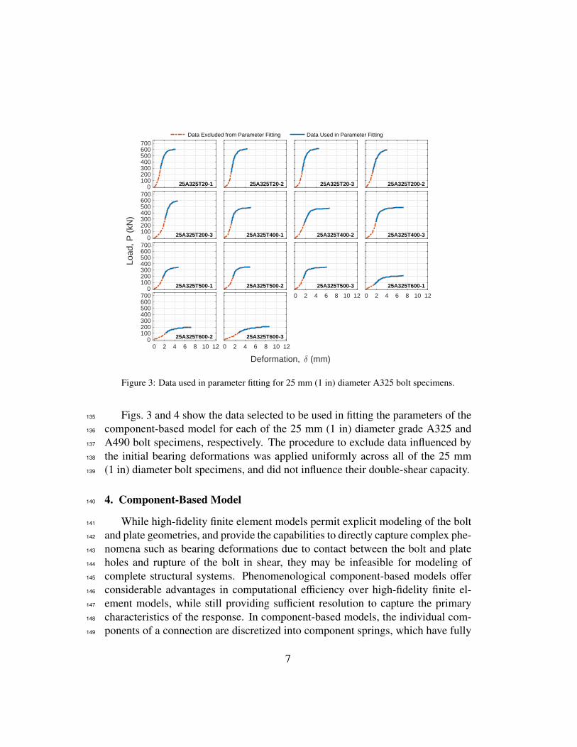
Figure 3: Data used in parameter fitting for 25 mm (1 in) diameter A325 bolt specimens.

Figs. 3 and 4 show the data selected to be used in fitting the parameters of the135

component-based model for each of the 25 mm (1 in) diameter grade A325 and136

A490 bolt specimens, respectively. The procedure to exclude data influenced by137

the initial bearing deformations was applied uniformly across all of the 25 mm138

(1 in) diameter bolt specimens, and did not influence their double-shear capacity.139

4. Component-Based Model140

While high-fidelity finite element models permit explicit modeling of the bolt141

and plate geometries, and provide the capabilities to directly capture complex phe-142

nomena such as bearing deformations due to contact between the bolt and plate143

holes and rupture of the bolt in shear, they may be infeasible for modeling of144

complete structural systems. Phenomenological component-based models offer145

considerable advantages in computational efficiency over high-fidelity finite el-146

ement models, while still providing sufficient resolution to capture the primary147

characteristics of the response. In component-based models, the individual com-148

ponents of a connection are discretized into component springs, which have fully149

7

Deformation, (mm)

Load

, P (

kN)

0100200300400500600700

25A490T20-1 25A490T20-2 25A490T20-3 25A490T20-4

0100200300400500600700

25A490T200-1 25A490T200-2 25A490T200-3 25A490T400-1

0100200300400500600700

25A490T400-2 25A490T400-3 25A490T500-1 25A490T500-2

0 2 4 6 8 10 120

100200300400500600700

25A490T500-3

0 2 4 6 8 10 12

25A490T600-1

0 2 4 6 8 10 12

25A490T600-2

0 2 4 6 8 10 12

25A490T600-3

Data Excluded from Parameter Fitting Data Used in Parameter Fitting

Figure 4: Data used in parameter fitting for 25 mm (1 in) diameter A490 bolt specimens.

8

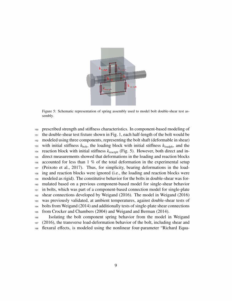
Figure 5: Schematic representation of spring assembly used to model bolt double-shear test as-sembly.

prescribed strength and stiffness characteristics. In component-based modeling of150

the double-shear test fixture shown in Fig. 1, each half-length of the bolt would be151

modeled using three components, representing the bolt shaft (deformable in shear)152

with initial stiffness kbolt, the loading block with initial stiffness kloadplt, and the153

reaction block with initial stiffness kreactplt (Fig. 5). However, both direct and in-154

direct measurements showed that deformations in the loading and reaction blocks155

accounted for less than 1 % of the total deformation in the experimental setup156

(Peixoto et al., 2017). Thus, for simplicity, bearing deformations in the load-157

ing and reaction blocks were ignored (i.e., the loading and reaction blocks were158

modeled as rigid). The constitutive behavior for the bolts in double-shear was for-159

mulated based on a previous component-based model for single-shear behavior160

in bolts, which was part of a component-based connection model for single-plate161

shear connections developed by Weigand (2016). The model in Weigand (2016)162

was previously validated, at ambient temperatures, against double-shear tests of163

bolts from Weigand (2014) and additionally tests of single-plate shear connections164

from Crocker and Chambers (2004) and Weigand and Berman (2014).165

Isolating the bolt component spring behavior from the model in Weigand166

(2016), the transverse load-deformation behavior of the bolt, including shear and167

flexural effects, is modeled using the nonlinear four-parameter “Richard Equa-168

9

tion”, which was formulated by Richard and Abbott (1975):169

P (δ) =

(ki − kp

)(δ − δ0)(

1 +

∣∣∣∣∣ (ki−kp)(δ−δ0)rn

∣∣∣∣∣n)(1/n) + kp (δ − δ0) (1)

where δ is the bolt shear deformation, δ0 is the initial bearing deformation, ki170

and kp are elastic and plastic stiffnesses of the bolt double-shear load-deformation171

response, respectively, n is a shape parameter that controls the sharpness of the172

transition from the elastic stiffness to the plastic stiffness, and rn is a reference173

load. Eq. (1) can be extended to include the effects of elevated temperatures on174

the bolt shear load-deformation response such that175

P (δ,T ) =

(ki(T ) − kp(T )

)(δ − δ0(T ))(

1 +

∣∣∣∣∣ (ki(T )−kp(T ))(δ−δ0(T ))rn(T )

∣∣∣∣∣n(T ))(1/n(T )) + kp(T ) (δ − δ0(T )) , (2)

where (T ) denotes dependence of the stiffness or capacity parameter on tem-176

perature. Where possible, temperature-dependence is included by incorporating177

temperature-dependent bolt steel mechanical properties directly into the equations178

describing the bolt response.179

4.1. Calculation of Equation Parameters180

While fitted values for the parameters in Eq. (2) were ultimately determined181

using optimization techniques, first-order approximations for the parameters (typ-182

ically within 10 % – 40 % of the globally optimized value, depending on the183

parameter) can be calculated based on linear least-squares regression of the bolt184

shear load-deformation data, since the Richard Equation has asymptotic limits of185

ki at δ = 0 and kp at δ = δu (where δu is the ultimate deformation of the bolt).186

These approximate values are used to initialize the optimization scheme, reducing187

its computational cost and increasing its likelihood of finding the globally optimal188

solution.189

Fig. 6 shows a graphical representation of the calculated first-order approxima-190

tions for a representative bolt double-shear load-deformation curve. An estimate191

for the initial stiffness of the bolt double-shear load-deformation response at tem-192

perature T , ki(T ), was already previously calculated (in Step 3 of the portion of193

the data used in fitting the parameters of the component-based model) as the slope194

10

of the linear least-squares regression of the bolt load-deformation data exceeding195

95 % of the peak slope. The initial bearing deformation is estimated as the value196

of the initial stiffness regression line at zero load, or197

δ0(T ) ≈ −bki(T )ki(T )

, (3)

where bki(T ) is the constant term of the linear regression. The plastic stiffness198

kp(T ) is calculated in a similar manner as the initial stiffness, but as the slope of the199

linear least-squares regression to the last four points of the bolt load-deformation200

response at the bolts’ maximum plastic deformations. The reference load corre-201

sponds to the projection of the plastic stiffness at a deformation of δ0(T ), and is202

thus calculated as203

rn(T ) ≈ bkp(T ) + kp(T )δ0(T ) (4)

where bkp(T ) is the constant term of the linear least-squares regression defining204

the plastic stiffness. The initial estimate of the shape parameter was determined205

using an iterative procedure to minimize the residual between Eq. (2) (using the206

already-fitted values for temperature-dependent initial stiffness ki(T ), plastic stiff-207

ness kp(T ), and reference load rn(T )), and the data from each individual bolt208

double-shear load-deformation curve.209

The globally optimal values for the parameters of Eq. (2) were determined210

using global optimization (a global search algorithm developed by Ugray et al.211

(2007) and available in MATLAB’s Global Optimization Toolbox (MathWorks,212

2016). This algorithm initially executes gradient-based local optimizations from213

a large number of starting points from within the parameter space, selecting the214

local optimization result with the minimum objective function value as the starting215

point to execute the final global optimization. The global search algorithm was216

initialized using the first-order approximations for the parameters in Eq. (2), which217

in effect scatters the starting points for the local optimizations in the vicinity of218

the initial point. Table 1 presents a summary of the final fitted parameters for each219

individual bolt specimen, and the parameter values are also shown graphically in220

Figs. 7 and 8 for the 25 mm (1 in) diameter A325 and A490 bolts, respectively.221

Replicate tests at each temperature level had relatively consistent double-shear222

capacities vn, within 4.5 % of the mean double-shear capacity value for all spec-223

imens. Thus, it follows that at each temperature level, the calculated values for224

the reference load rn are closely grouped, having the least scatter of the four cal-225

culated curve parameters. For both the A325 and A490 bolts, the reference load226

was only slightly degraded for temperatures up to 200 °C, with more significant227

11

Table 1: Summary of measured and fitted curve parameters for bolt shear data.

Specimen T ki(T ) kp(T ) kp(T )/ki(T ) rn(T ) vn(T ) n(T ) δ0Name °C kN/m (kip/in) kN/m (kip/in) - kN (kip) kN (kip) - mm (in)

25A325T20-1 20 406246 (2319.7) 9649 (55.1) 0.024 574.1 (129.1) 606.7 (136.4) 4.11 0.46 (0.018)25A325T20-2 20 563716 (3218.9) 9211 (52.6) 0.016 583.7 (131.2) 612.4 (137.7) 3.11 0.84 (0.033)25A325T20-3 20 531428 (3034.5) 6938 (39.6) 0.013 594.8 (133.7) 617.0 (138.7) 3.20 0.83 (0.033)25A325T200-2 200 403817 (2305.9) 12959 (74.0) 0.032 565.7 (127.2) 598.7 (134.6) 3.21 0.64 (0.025)25A325T200-3 200 447788 (2556.9) 13990 (79.9) 0.031 557.4 (125.3) 594.2 (133.6) 3.48 1.42 (0.056)25A325T400-1 400 631536 (3606.2) 7541 (43.1) 0.012 461.4 (103.7) 489.7 (110.1) 2.37 0.89 (0.035)25A325T400-2 400 219143 (1251.3) 3205 (18.3) 0.015 455.6 (102.4) 474.6 (106.7) 5.76 0.63 (0.025)25A325T400-3 400 581838 (3322.4) 3361 (19.2) 0.006 475.4 (106.9) 491.6 (110.5) 2.11 1.34 (0.053)25A325T500-1 500 235309 (1343.6) 7358 (42.0) 0.031 315.8 (71.0) 342.6 (77.0) 4.05 0.92 (0.036)25A325T500-2 500 349763 (1997.2) 5968 (34.1) 0.017 329.8 (74.1) 352.3 (79.2) 3.32 1.07 (0.042)25A325T500-3 500 317683 (1814.0) 2633 (15.0) 0.008 331.1 (74.4) 343.6 (77.3) 3.02 0.97 (0.038)25A325T600-1 600 90775 (518.3) 2082 (11.9) 0.023 194.1 (43.6) 206.3 (46.4) 3.58 0.80 (0.032)25A325T600-2 600 162149 (925.9) 2658 (15.2) 0.016 188.4 (42.3) 197.2 (44.3) 1.73 1.45 (0.057)25A325T600-3 600 110453 (630.7) 2551 (14.6) 0.023 200.4 (45.1) 208.7 (46.9) 1.72 1.41 (0.055)

Average - 360832 (2060.4) 6436 (36.8) 0.019 416.3 (93.6) 438.3 (98.5) 3.20 0.98 (0.038)

25A490T20-1 20 475164 (2713.3) 15106 (86.3) 0.032 652.5 (146.7) 696.2 (156.5) 4.54 0.42 (0.016)25A490T20-2 20 523028 (2986.6) 19773 (112.9) 0.038 643.1 (144.6) 687.9 (154.6) 3.99 0.97 (0.038)25A490T20-3 20 509413 (2908.8) 11016 (62.9) 0.022 664.2 (149.3) 696.3 (156.5) 3.70 0.87 (0.034)25A490T20-4 20 552313 (3153.8) 12526 (71.5) 0.023 657.9 (147.9) 691.7 (155.5) 3.72 0.47 (0.019)25A490T200-1 200 458405 (2617.6) 16297 (93.1) 0.036 632.7 (142.2) 680.1 (152.9) 3.90 1.05 (0.041)25A490T200-2 200 389630 (2224.8) 20583 (117.5) 0.053 622.3 (139.9) 689.6 (155.0) 4.23 1.06 (0.042)25A490T200-3 200 467048 (2666.9) 10292 (58.8) 0.022 650.3 (146.2) 680.2 (152.9) 3.84 0.70 (0.027)25A490T400-1 400 597447 (3411.5) 7078 (40.4) 0.012 544.1 (122.3) 574.2 (129.1) 2.73 1.13 (0.044)25A490T400-2 400 393286 (2245.7) 7044 (40.2) 0.018 532.4 (119.7) 557.8 (125.4) 4.02 0.98 (0.039)25A490T400-3 400 456413 (2606.2) 9955 (56.8) 0.022 515.3 (115.8) 560.8 (126.1) 3.57 1.04 (0.041)25A490T500-1 500 337725 (1928.5) 6022 (34.4) 0.018 386.4 (86.9) 411.0 (92.4) 3.85 1.16 (0.046)25A490T500-2 500 263709 (1505.8) 4697 (26.8) 0.018 398.6 (89.6) 413.6 (93.0) 4.20 1.52 (0.060)25A490T500-3 500 323106 (1845.0) 4520 (25.8) 0.014 400.4 (90.0) 417.6 (93.9) 3.55 1.45 (0.057)25A490T600-1 600 79396 (453.4) 1352 (7.7) 0.017 243.8 (54.8) 247.0 (55.5) 1.85 0.92 (0.036)25A490T600-2 600 96121 (548.9) 3417 (19.5) 0.036 251.0 (56.4) 280.3 (63.0) 1.72 1.44 (0.057)25A490T600-3 600 89212 (509.4) 4775 (27.3) 0.054 220.9 (49.7) 279.4 (62.8) 1.79 1.51 (0.060)

Average - 375714 (2145.4) 9653 (55.1) 0.027 501.0 (112.6) 535.2 (120.3) 3.45 1.04 (0.041)

12

0.0 0.5 1.0 1.5 2.0 2.5 3.0 3.5 4.0 4.5

Deformation, (mm)

0

100

200

300

400

500

600Lo

ad, P

(kN

)

0

rn

kik

p

u

Pu

Figure 6: First-order approximation of Richard Equation parameters.

degradation at 400 °C and above. These trends are consistent with observations by228

Yu (2006), who also found that high-strength bolts did not experience significant229

degradation in strength at temperatures less than 300 °C.230

The other three curve parameters had more scatter in their calculated values for231

a given temperature. In general, both the initial stiffness and the plastic stiffness of232

the bolt shear load-deformation curves tended to degrade with increasing temper-233

ature. The calculated values for the shape parameter n were usually grouped at a234

particular temperature; but no systematic trend in their magnitudes with respect to235

temperature was observed. For both bolt grades, the value of the shape parameter236

at all temperatures was between 1.5 and 6.0. The scatter in the calculated values237

of the initial stiffness ki, plastic stiffness kp, and shape parameter n at each tem-238

perature level did not appear to be adversely influenced by increased temperature,239

with the scatter in the calculated parameter values at ambient temperature often240

exceeding that at 600 °C.241

Figs. 9(a) and 9(b) show a comparison between Eq. (2) using the parameters242

fitted via global optimization with data from the 25 mm (1 in) diameter A325243

and A490 bolts, respectively, with the initial bearing deformations δ0 from each244

test removed for clarity. Fig. 9 shows that use of Eq. (2) with the fitted curve245

13

0 100 200 300 400 500 600

Temperature (°C)

0

1

2

3

4

5

6

7

Initi

al S

tiffn

ess,

ki (

kN/m

m)

105

(a)

0 100 200 300 400 500 600

Temperature (°C)

0.2

0.4

0.6

0.8

1

1.2

1.4

Pla

stic

Stif

fnes

s, k

p (kN

/m)

104

(b)

0 100 200 300 400 500 600

Temperature (°C)

100

200

300

400

500

600

Ref

eren

ce L

oad,

rn (

kN)

(c)

0 100 200 300 400 500 600

Temperature (°C)

0

1

2

3

4

5

6

7

Sha

pe P

aram

eter

, n

(d)

Figure 7: Values of fitted curve parameters for 25 mm (1 in) diameter A325 bolts as a function oftemperature: (a) initial stiffness ki(T ), (b) plastic stiffness kp(T ), (c) reference load rn(T ), and (d)shape parameter n(T ) (unitless).

14

0 100 200 300 400 500 600

Temperature (°C)

0

1

2

3

4

5

6

Initi

al S

tiffn

ess,

ki (

kN/m

m)

105

(a)

0 100 200 300 400 500 600

Temperature (°C)

0

0.5

1

1.5

2

2.5

Pla

stic

Stif

fnes

s, k

p (kN

/m)

104

(b)

0 100 200 300 400 500 600

Temperature (°C)

200

300

400

500

600

700

Ref

eren

ce L

oad,

rn (

kN)

(c)

0 100 200 300 400 500 600

Temperature (°C)

0

1

2

3

4

5

6

Sha

pe P

aram

eter

, n

(d)

Figure 8: Values of fitted curve parameters for 25 mm (1 in) diameter A490 bolts as a function oftemperature: (a) initial stiffness ki(T ), (b) plastic stiffness kp(T ), (c) reference load rn(T ), and (d)shape parameter n(T ) (unitless).

15

0 1 2 3 4 5 6 7 8 9 10 11 12 13 14

Deformation, (mm)

0

50

100

150

200

250

300

350

400

450

500

550

600

650

700

Load

, P (

kN)

Bolt Double-Shear DataEq. (2) with Fitted Parameters

(a)

0 1 2 3 4 5 6 7 8 9 10 11 12 13 14

Deformation, (mm)

0

50

100

150

200

250

300

350

400

450

500

550

600

650

700

Load

, P (

kN)

Bolt Double-Shear DataEq. (2) with Fitted Parameters

(b)

Figure 9: Comparison between Eq. (1) using fitted curve parameters and experimental data for25 mm (1 in) diameter (a) A325 bolts and (b) A490 bolts.

parameters provided in Table 1 matches the experimental data within 3 % across246

all bolt tests.247

4.2. Temperature-Dependent Models for Bolt Mechanical Properties248

To develop an approach that can predict the shear load-deformation response249

of the 19 mm (3/4 in) and 22 mm (7/8 in) diameter bolts using the data from250

the 25 mm (1 in) bolts, the bolt-shear component-based model from Weigand251

(2016) is used to transform the reference load and initial stiffness data into the252

ultimate tensile strength and modulus of elasticity, respectively, of the bolt steel.253

Next, equations are fitted to the data for the ultimate tensile strength and modulus254

of elasticity, providing temperature-dependent expressions for these mechanical255

properties, which should be relatively consistent between bolts of different diam-256

eters. Piece-wise linear equations are also fitted to the data for the plastic stiffness257

and shape parameter to facilitate complete double-shear modeling of the bolt re-258

sponse at elevated temperatures.259

The ultimate tensile strength of the bolt steels, Fu(T ), can be related to the260

shear capacity via the equation for the temperature-dependent double-shear ca-261

pacity of the bolt, vn(T ) = nsp0.6AbFu(T ), where nsp = 2 is the number of shear262

planes through the bolt, and Ab = (π/4) d2b is the bolt cross-sectional area. The bolt263

steel ultimate tensile strength can be written in terms of the double-shear capacity264

16

0 100 200 300 400 500 600

Temperature (°C)

0

200

400

600

800

1000

1200

Fu (

MP

a)

Ultimate Tensile Strength DataNonlinear Regression (using Eq. (6))95 % Confidence Bounds

(a)

0 100 200 300 400 500 600

Temperature (°C)

0

200

400

600

800

1000

1200

Fu (

MP

a)

Ultimate Tensile Strength DataNonlinear Regression (using Eq. (6))95 % Confidence Bounds

(b)

Figure 10: Ultimate tensile strength, fitted using Eq. (6), for 25 mm (1 in) diameter (a) A325 boltsand (b) A490 bolts. Hatched area corresponds to 95 % confidence interval.

of the bolt such that265

Fu(T ) =vn(T )

nsp0.6Ab. (5)

The discrete markers in Fig. 10 show the values for the ultimate tensile strength266

calculated using Eq. (5).267

To characterize the ultimate tensile strength over the full range of temperatures268

of interest, an exponential function of the form:269

Fu,fitted(T ) = Fu,amb

(a1 + (1 − a1) exp

(−

12

((T − Tamb

a2

)a3

+

(T − Tamb

a2

)a4)))

(6)

was fitted to the experimental data using nonlinear least-squares regression tech-270

niques (Fig. 10). The ambient-temperature ultimate tensile strength Fu,amb was fit-271

ted to the data along with the other coefficients. The fitted coefficients of Eq. (6),272

Fu,amb and a1 through a4, are shown in Table 2 along with their 95 % confidence273

bounds. The 95 % confidence bounds are also shown on Fig. 10 as dashed lines,274

with the hatched area between the confidence bounds comprising the 95 % con-275

fidence interval. The 95 % confidence bounds form a narrow band enclosing the276

respective fits to the ultimate tensile strength data, indicating that the variance in277

the measured ultimate tensile strengths is relatively small.278

Independent tensile testing of coupons machined from the 25 mm (1 in) di-279

ameter A325 and A490 bolts measured the ambient-temperature ultimate tensile280

strengths for the A325 and A490 bolts at 950.9 MPa (137.9 ksi) and 1126.7 MPa281

(163.4 ksi), respectively, which are within 6 % and 1 %, of the values of Fu,amb282

17

Table 2: Summary of fitted curve parameters for bolt mechanical properties.

Grade A325 Grade A490

95 % Confidence 95 % ConfidenceFit Type Coeff. Value Bounds (lower, upper) Coeff. Value Bounds (lower, upper) units

Fu,amb = 1007 (146.0)(993 (144.0), 1020 (148.0)

)Fu,amb = 1140 (165.3)

(1122 (162.8), 1157 (167.8)

)MPa (ksi)

Ultimate Tensile a1 = 0.2758(0.1591, 0.3925

)a1 = 0.3141

(0.1211, 0.5072

)°C

Strength (Eq. (6)) a2 = 488.7(456.9, 520.5

)a2 = 492.7

(435.3, 550.2

)°C

a3 = 7.291(3.924, 10.659

)a3 = 6.251

(0.766, 11.736

)-

a4 = 2.649(1.767, 3.531

)a4 = 3.207

(1.334, 5.079

)-

Eamb = 170.13 (24675)(118.92 (17248), 221.34 (32102)

)Eamb = 175.47 (25450)

(154.39 (22392), 196.56 (28508)

)GPa (ksi)

Modulus of g1 = -0.0004083(-0.0011032, 0.0002867

)g1 = -0.0004835

(-0.0007801, -0.0001869

)°C−3

Elasticity (Eq. (14)) g2 = 0.2631(-0.3700, 0.8962

)g2 = 0.3184

(0.0551, 0.5818

)°C−2

g3 = -48.48(-197.69, 100.73

)g3 = -59.25

(-119.67, 1.18

)°C−1

fitted to the bolt double-shear data. The close agreement between the fitted values283

and measured ultimate tensile strengths at ambient temperature provides evidence284

that Eq. (5) is appropriate, and lends credibility to the approach of using the more285

numerous (in the current study) double-shear strength data to estimate the ultimate286

tensile strength of the bolt materials.287

The modulus of elasticity of the bolt steels can be related to the initial stiffness288

of the bolts using Eq. (20) from Weigand (2016), but adjusted for the two shear289

planes through the bolt in double-shear testing, and incorporating temperature-290

dependence such that:291

ki(T ) =nsp

1kbr(T ) + 1

kv(T )

, (7)

with bearing stiffness292

kbr(T ) =1

1 + 3βb

(tRBtLBE(T )2 (tRB + tLB)

), (8)

and shearing stiffness293

kv(T ) =12E(T )Ib

L3b(1 + Φ(T ))

. (9)

In Eqs. (8) and (9), βb is a correction factor that accounts for the concentration of294

bearing forces at the interface between plates (βb = 1 for shear was used in this295

study, see Nelson et al. (1983) for more details), Ib =(πd4

b

)/64 is the moment of296

inertia of the bolt shaft cross-section, Lb = (1/2) (tRB + tLB) is the bolt length at297

each shear plane where tRB=30 mm (1.18 in) is the thickness of the reaction block,298

18

and where tLB=56 mm (2.20 in) is the thickness of the loading block.299

Φ(T ) =12E(T )Ib

L2b

(1

κG(T )Ab

)(10)

is a term in Timoshenko beam theory that characterizes the relative importance300

of the shear deformations to the bending deformations (e.g., see Thomas et al.301

(1973)), G(T ) = E(T )/ (2 (1 + ν)) is the bolt shear modulus, ν = 0.29 (assumed302

over all temperatures) is Poisson’s ratio, and κ is the shear coefficient for a circular303

cross-section, defined as:304

κ =1

76 + 1

6

(ν

1+ν

)2 . (11)

The modulus of elasticity of the bolt steel is determined by solving Eq. (7) for305

E(T ) such that:306

E(T ) = γki(T ) , (12)

where307

γ =2(tRB + tLB)

(3 (1 + 3βb) πd4

b (1 + ν) + d2b(7 + 2ν(7 + 4ν))tRBtLB + (1 + ν) tRBtLB (tRB + tLB)2

)nsp

(3πd4

b(1 + ν)tRBtLB

) .

(13)Similar to the approach taken for the ultimate tensile strength, an equation was308

fitted to the modulus of elasticity data to enable its calculation for all temperatures.309

For the modulus of elasticity, a third-order polynomial equation of the form:310

Efitted(T ) = Eamb

(g1(T − Tamb)3 + g2(T − Tamb)2 + g3(T − Tamb) + 1

)(14)

was fitted to the experimental data using least-squares regression techniques. Co-311

efficients g1 through g4 are shown in Table 2. Fitted curves using Eq. (14) are312

shown in Fig. 11 as solid lines. As a result of the larger variances in the modulus313

of elasticity data, the 95 % confidence intervals calculated for the fitted modulus314

of elasticity curves are significantly wider than those calculated for the ultimate315

tensile strength.316

Due to the significant scatter in the data for the plastic stiffness (see Figs. 7(b)317

and 8(b)), a different approach was used to calculate it. The relationship between318

the plastic stiffness and the elastic stiffness, at a particular temperature, was de-319

termined as the average of the kp(T )/ki(T ) values from Table 1 (Fig. 12), and the320

plastic stiffness was calculated as this ratio multiplied by specimen-specific initial321

stiffness. The shape parameter n, while influencing the bolt double-shear response322

19

0 100 200 300 400 500 600

Temperature (°C)

0

50

100

150

200

E (

GP

a)

Modulus of Elasticity DataNonlinear Regression (using Eq. (14))95 % Confidence Bounds

(a)

0 100 200 300 400 500 600

Temperature (°C)

0

50

100

150

200

E (

GP

a)

Modulus of Elasticity DataNonlinear Regression (using Eq. (14))95 % Confidence Bounds

(b)

Figure 11: Modulus of elasticity, fitted using Eq. (14), for 25 mm (1 in) diameter (a) A325 boltsand (b) A490 bolts. Hatched area corresponds to 95 % confidence interval.

at the transition from elastic to plastic deformations, has relatively little influence323

on the calculated capacity of the bolts. Thus, the value of n was simply chosen324

as the average value at each individual temperature. The data from Peixoto et al.325

(2017) showed no systematic influence of bolt diameter of the double-shear de-326

formation at failure, and thus the deformations at failure was similarly chosen as327

the average value at each temperature. Since the stiffness of the bolt double-shear328

response had significantly decreased at the ultimate deformations, choosing aver-329

aged values for the ultimate deformation capacities had only a minor influence on330

the calculated bolt reference loads.331

Figs. 14(a) and 14(b) show comparisons of the component-based model, with332

parameters fitted using Eq. (6), Eq. (14), and the approaches for calculating kp and333

n described above, to the experimental data for the 25 mm (1 in) diameter bolts.334

5. Application of Modeling Approach to Smaller-Diameter Bolts335

The empirical bolt load-deformation modeling approach is based solely on the336

data from Peixoto et al. (2017) for the 25 mm (1 in) diameter A325 and A490337

bolts. In this section, the capabilities of the modeling approach in predicting338

temperature-dependent capacities for the bolts are tested against data from the339

19 mm (3/4 in) and 22 mm (7/8 in) diameter bolts in Peixoto et al. (2017). It is340

challenging to directly compare the load-deformation responses for the bolts, due341

to the effects of excessive bearing deformations in the loading and reaction blocks342

used for the 19 mm (3/4 in) and 22 mm (7/8 in) diameter bolt tests (as described343

in Section 2). As an example, Fig. 15 shows the effect of the accumulated bearing344

20

0 100 200 300 400 500 600

Temperature (°C)

0

0.01

0.02

0.03

0.04

0.05

0.06

k p /

k i

(a)

0 100 200 300 400 500 600

Temperature (°C)

0

0.01

0.02

0.03

0.04

0.05

0.06

k p /

k i(b)

Figure 12: Fitted ratio of plastic stiffness to initial stiffness for 25 mm (1 in) diameter (a) A325bolts and (b) A490 bolts.

0 100 200 300 400 500 600

Temperature (°C)

0

1

2

3

4

5

6

n

(a)

0 100 200 300 400 500 600

Temperature (°C)

0

1

2

3

4

5

6

n

(b)

Figure 13: Fitted shape parameter for 25 mm (1 in) diameter (a) A325 bolts and (b) A490 bolts.

21

0 1 2 3 4 5 6 7 8 9 10 11 12 13 14

Deformation (mm)

0

50

100

150

200

250

300

350

400

450

500

550

600

650

700

Load

(kN

)

Component-based ModelExp. Data at T = 20 °CExp. Data at T = 200 °CExp. Data at T = 400 °CExp. Data at T = 500 °CExp. Data at T = 600 °C

(a)

0 1 2 3 4 5 6 7 8 9 10 11 12 13 14

Deformation (mm)

0

50

100

150

200

250

300

350

400

450

500

550

600

650

700

Load

(kN

)

Component-based ModelExp. Data at T = 20 °CExp. Data at T = 200 °CExp. Data at T = 400 °CExp. Data at T = 500 °CExp. Data at T = 600 °C

(b)

Figure 14: Comparison of component-based model to experimental data for 25 mm (1 in) diameter(a) A325 bolts and (b) A490 bolts.

deformations by comparing results from the first 19 mm (3/4 in) diameter bolt test345

(19A325T20-1), in which the virgin loading and reaction blocks were used, with346

results from the third 19 mm (3/4 in) diameter bolt test (19A325T20-3). However,347

since the accumulated bearing deformations had relatively little influence on the348

bolt double-shear capacity (as demonstrated by Fig. 15), the double-shear capac-349

ities of the 19 mm (3/4 in) and 22 mm (7/8 in) diameter bolts can be objectively350

compared.351

The bolts are modeled using Eq. (2), with (i) initial stiffness determined from352

Eq. (7), incorporating temperature-dependence via Eq. (14) (Fig. 11) for the mod-353

ulus of elasticity, (ii) plastic stiffness determined as a function of the initial stiff-354

ness, using the ratios shown in Fig. 12, (iii) shape parameter taken as the average355

value at each temperature (see Fig. 13), and reference load calculated as356

rn = nsp0.6AbFu(T ) (δu − δ0) (15)

using the fitted ultimate tensile strength (Eq. (6), Fig. 10). The bolt-shear deforma-357

tion capacities at failure were assumed to be equivalent to the average deformation358

capacities of the corrected 25 mm (1 in) diameter bolt data.359

Tables 3 and 4 show that the empirically-fitted modeling approach predicts360

the capacity of the 19 mm (3/4 in) and 22 mm (7/8 in) bolts within an average361

difference of less than 3.5 %. A negative value for the percent error indicates that362

22

Table 3: Summary of measured and predicted double-shear capacities for 19 mm (3/4 in) and22 mm (7/8 in) diameter A325 high-strength bolts.

Specimen T Meas. Failure Pred. Failure PercentName °C Load, kN (kip) Load, kN (kip) Difference

19A325T20-1 20 372.3 (83.7) 379.9 (85.4) 2.019A325T20-2 20 375.4 (84.4) 1.219A325T20-3 20 391.9 (88.1) -3.119A325T200-1 200 384.3 (86.4) 370.2 (83.2) -3.719A325T200-2 200 392.3 (88.2) -5.619A325T200-3 200 388.8 (87.4) -4.819A325T400-1 400 310.0 (69.7) 301.2 (67.7) -2.819A325T400-2 400 312.3 (70.2) -3.519A325T400-3 400 314.5 (70.7) -4.219A325T500-1 500 218.0 (49.0) 214.9 (48.3) -1.419A325T500-2 500 232.6 (52.3) -7.619A325T500-3 500 216.6 (48.7) -0.819A325T600-1 600 122.3 (27.5) 126.6 (28.5) 3.519A325T600-2 600 134.8 (30.3) -6.019A325T600-3 600 124.1 (27.9) 2.0

|Average| - - - 3.5

22A325T20-1 20 540.5 (121.5) 533.1 (119.8) -1.422A325T20-2 20 528.0 (118.7) 1.022A325T20-3 20 540.5 (121.5) -1.422A325T20-4 20 523.6 (117.7) 1.822A325T200-1 200 503.5 (113.2) 519.5 (116.8) 3.222A325T200-2 200 514.2 (115.6) 1.022A325T200-3 200 517.8 (116.4) 0.322A325T400-1 400 464.4 (104.4) 422.7 (95.0) -9.022A325T400-2 400 443.0 (99.6) -4.622A325T400-3 400 444.4 (99.9) -4.922A325T500-1 500 332.7 (74.8) 301.6 (67.8) -9.422A325T500-2 500 304.3 (68.4) -0.922A325T500-3 500 294.5 (66.2) 2.422A325T600-1 600 172.1 (38.7) 177.7 (40.0) 3.222A325T600-2 600 182.8 (41.1) -2.822A325T600-3 600 179.3 (40.3) -0.9

|Average| - - - 3.0

23

Table 4: Summary of measured and predicted double-shear capacities for 19 mm (3/4 in) and22 mm (7/8 in) diameter A490 high-strength bolts.

Specimen T Meas. Failure Pred. Failure PercentName °C Load, kN (kip) Load, kN (kip) Difference

19A490T20-1 20 414.6 (93.2) 419.6 (94.3) 1.219A490T20-2 20 415.0 (93.3) 1.119A490T20-3 20 429.3 (96.5) -2.219A490T200-1 200 412.4 (92.7) 413.7 (93.0) 0.319A490T200-2 200 398.6 (89.6) 3.819A490T200-3 200 420.4 (94.5) -1.619A490T400-1 400 347.4 (78.1) 341.7 (76.8) -1.719A490T400-2 400 355.0 (79.8) -3.719A490T400-3 400 364.8 (82.0) -6.319A490T500-1 500 258.4 (58.1) 250.7 (56.4) -3.019A490T500-2 500 262.9 (59.1) -4.619A490T500-3 500 259.3 (58.3) -3.319A490T600-1 600 158.4 (35.6) 162.8 (36.6) 2.819A490T600-2 600 163.7 (36.8) -0.519A490T600-3 600 161.0 (36.2) 1.1

|Average| - - - 2.5

22A490T20-1 20 568.5 (127.8) 577.2 (129.8) 1.522A490T20-2 20 575.2 (129.3) 0.422A490T20-3 20 588.1 (132.2) -1.822A490T200-1 200 537.8 (120.9) 569.1 (127.9) 5.822A490T200-2 200 549.4 (123.5) 3.622A490T200-3 200 555.6 (124.9) 2.422A490T400-1 400 480.9 (108.1) 470.0 (105.7) -2.322A490T400-2 400 450.2 (101.2) 4.422A490T400-3 400 466.6 (104.9) 0.722A490T500-1 500 357.2 (80.3) 344.9 (77.5) -3.522A490T500-2 500 352.7 (79.3) -2.222A490T500-3 500 363.0 (81.6) -5.022A490T600-1 600 206.4 (46.4) 223.9 (50.3) 8.522A490T600-2 600 214.8 (48.3) 4.222A490T600-3 600 224.2 (50.4) -0.1

|Average| - - - 3.1

24

0 0.5 1 1.5 2 2.5 3 3.5 4 4.5 5 5.5 6 6.5 7

Deformation (mm)

0

50

100

150

200

250

300

350

400

450

500

Load

(kN

)

19A325T20-119A325T20-3Model Prediction (no bearing deformations)

Figure 15: Effect of accumulated bearing deformations on 19 mm (3/4 in) diameter bolt tests.

the predicted double-shear capacity is larger than the experimentally measured363

double shear capacity, while a positive value for the percent error indicates that364

the predicted double-shear capacity is smaller than the experimentally measured365

double shear capacity. The reported averages in Tables 3 and 4 correspond to the366

average of the absolute value of the percent differences across the full range of367

test temperatures.368

Tables 3 and 4 also show that the percent difference between the predicted369

bolt double-shear capacity and the measured bolt double-shear capacity tends to370

increase with increasing temperature, with the predicted capacities at 500 °C and371

600 °C on-average having the largest percent differences. This trend could be372

rationally expected, due to contributions from the combined uncertainties in the373

deformation at failure and the plastic stiffness in the measured data at these tem-374

peratures.375

6. Consolidation and Simplification of Component-Based Model376

With only a minor loss of accuracy relative to the separately fitted models for377

the grade A325 and A490 high-strength bolt materials presented in Section 4.2,378

the component-based model can be consolidated to a single model that is applica-379

ble to both types of high-strength bolts. Fig. 16(a) shows a comparison between380

the retained ultimate tensile strengths for the grade A325 and A490 bolt materi-381

als. The retained mechanical properties of the bolt materials are calculated simply382

as the values of the mechanical properties at elevated temperatures normalized383

by their mean value at ambient temperature, µFu,amb . Both material grades exhibit384

25

0 100 200 300 400 500 600

Temperature (°C)

0

0.2

0.4

0.6

0.8

1

Fu /

Fu,

amb

A325 Bolt DataA325 Bolt Material FitA490 Bolt DataA490 Bolt Material Fit

(a)

0 100 200 300 400 500 600

Temperature (°C)

0

0.2

0.4

0.6

0.8

1

Ret

aine

d F

u

Ultimate Tensile Strength DataNonlinear Regression (using Eq. (6))95 % Confidence Bounds

Fitted Parameters for Eq. (6):

a1 = 1.000 (0.985, 1.015)

a2 = 0.290 (0.114, 0.466)

a3 = 491.9 (441.8, 542.0)

a4 = 6.650 (1.986, 11.315)

a5 = 2.942 (1.565, 4.320)

(b)

Figure 16: (a) comparison of individually fitted retained ultimate tensile strength curves for 25 mm(1 in) diameter grade A325 and A490 bolts and (b) aggregated ultimate tensile strength, fitted usingEq. (6).

similar trends, having relatively little degradation at 200 °C after which the rate of385

degradation increases with increasing temperature. Clearly, the retained ultimate386

tensile strength of the grade A325 bolt material is less than that of the grade A490387

bolt material, indicating that the grade A325 bolt material degraded faster than the388

grade A490 bolt material with increasing temperature. However, the difference in389

the retained ultimate tensile strengths of the two bolt materials is relatively mi-390

nor, differing by only 5.5 % at the maximum considered temperature of 600 °C391

(the ultimate tensile strength of the grade A325 and A490 bolt materials were on392

average, 33.3 % and 38.8 %, respectively, of their ambient-temperature ultimate393

tensile strengths). Fig. 16(b) shows the consolidated fit to the bolt ultimate tensile394

strength data results, determined by fitting Eq. (6) to the aggregated data for both395

the grade A325 and A490 bolt materials. The fitted coefficients, a1 through a5,396

along with their 95 % confidence bounds, are shown in the textbox embedded in397

Fig. 16(b).398

A similar consolidation strategy can be considered for the modulus of elastic-399

ity data. Fig. 17(a) shows a comparison between the retained modulus of elasticity400

of the grade A325 and A490 bolt materials. The fitted curves for the modulus of401

elasticity show that for both bolt materials, the modulus is degraded only slightly402

at or below 400 °C, but then begins to degrade rapidly at temperatures above403

400 °C. At 600 °C, the retained modulus of elasticity of the grade A325 and404

26

0 100 200 300 400 500 600

Temperature (°C)

0

0.2

0.4

0.6

0.8

1

1.2

E /

Eam

b

A325 Bolt DataA325 Bolt Material FitA490 Bolt DataA490 Bolt Material Fit

(a)

0 100 200 300 400 500 600

Temperature (°C)

0

0.2

0.4

0.6

0.8

1

1.2

Ret

aine

d E

Retained Modulus of Elasticity DataNonlinear Regression (using Eq. (6))95 % Confidence Bounds

Fitted Parameters for Eq. (14):

p1 = -1.79e-08 (-3.00e-08, -5.75e-09)

p2 = 1.17e-05 (7.92e-07, 2.26e-05)

p3 = -0.00217 (-0.00471, 0.00036)

p4 = 1.000 (0.872, 1.128)

(b)

Figure 17: (a) comparison of individually fitted retained modulus of elasticity curves for 25 mm(1 in) diameter grade A325 and A490 bolts and (b) aggregated modulus of elasticity, fitted usingEq. (14).

A490 bolt materials were on average, 24.3 % and 17.2 %, respectively, of their405

ambient-temperature values. Despite the obvious scatter in the modulus of elas-406

ticity data, particularly for the tests at 400 °C, both the fitted retained modulus407

of elasticity curves for two bolt materials are barely distinguishable from one an-408

other. The close proximity of these two curves indicates that the bolt grade does409

not significantly influence the modulus of elasticity, even at elevated temperatures.410

Fig. 17(b) shows the fit of Eq. (14) to the aggregated bolt modulus of elasticity411

data for both the grade A325 and A490 bolt materials, with the fitted coefficients412

and their 95 % confidence bounds shown in the textbox.413

It was previously noted in Section 4.2 that the shape parameter n had rela-414

tively little influence on the calculated capacity of the bolts. The shape parame-415

ter likewise has relatively little influence on the initial response of the bolt load-416

deformation behavior, before appreciable plastic deformations have occurred. To417

simplify the formulation of the consolidated component-based model, the shape418

parameter is approximated as a constant value over all temperatures, and is cal-419

culated as the average of the consolidated shape parameter data from both the420

grade A325 and A490 bolts (Fig. 18(a)). A similar strategy is adopted for the421

ratio of the plastic stiffness to the initial stiffness (Fig. 18(b)). Use of average422

values for the shape parameter and stiffness ratio reduces the dependence of the423

component-based model on temperature. The consolidated simplified component-424

27

0 100 200 300 400 500 600

Temperature (°C)

0

1

2

3

4

5

6

Sha

pe P

aram

eter

, n

n = 3.33

A325 Bolt DataA490 Bolt Data

(a)

0 100 200 300 400 500 600

Temperature (°C)

0

0.01

0.02

0.03

0.04

0.05

0.06

Stif

fnes

s R

atio

, kp/k

i

n = 0.023

A325 Bolt DataA490 Bolt Data

(b)

Figure 18: Aggregated 25 mm (1 in) diameter grade A325 and A490 bolt data for (a) shapeparameter, and (b) ratio of plastic stiffness to initial stiffness.

based model depends only the temperature-dependent retained ultimate tensile425

strength and the temperature-dependent retained modulus of elasticity.426

Fig. 19 shows the predicted bolt double-shear load-deformation behavior from427

the consolidated component-based model, using the fitted curves to the retained428

ultimate tensile strength (Fig. 16(b)), retained modulus of elasticity (Fig. 17(b)),429

average shape parameter (Fig. 18(a)), and average stiffness ratio (Fig. 18(b)).430

Comparison of Fig. 14 and Fig. 19 shows that using the consolidated ultimate431

tensile strength and modulus of elasticity data, with average values for the shape432

parameter and stiffness ratio, results in only a slight loss of accuracy with respect433

to the measured bolt double-shear load-deformation responses. Even when using434

the simplified component-based model, the predicted response is still typically435

within the area bounded by the responses of the nominally identical tests. Where436

the simplified component-based model does predict loads outside the variation437

between nominal identical tests is typically only at the peak bolt deformation,438

where the predicted response differs from the nearest experimental response by a439

maximum of 6.5 % for the grade A325 bolts and 8.4 % for the grade A490 bolts.440

7. Assumptions and Limitations441

The component-based modeling approach presented in this paper assumed that442

the deformations in the loading and reaction blocks are sufficiently small to be ne-443

glected, and that deformations are concentrated in the bolt in the vicinity of the444

lapped joints. Since only a small portion of the deformations went into the load-445

ing block and reaction blocks (less than 1 % for tests at temperatures up to the446

28

0 1 2 3 4 5 6 7 8 9 10 11 12 13 14

Deformation (mm)

0

50

100

150

200

250

300

350

400

450

500

550

600

650

700

Load

(kN

)

Component-based ModelExp. Data at T = 20 °CExp. Data at T = 200 °CExp. Data at T = 400 °CExp. Data at T = 500 °CExp. Data at T = 600 °C

(a)

0 1 2 3 4 5 6 7 8 9 10 11 12 13 14

Deformation (mm)

0

50

100

150

200

250

300

350

400

450

500

550

600

650

700

Load

(kN

)

Component-based ModelExp. Data at T = 20 °CExp. Data at T = 200 °CExp. Data at T = 400 °CExp. Data at T = 500 °CExp. Data at T = 600 °C

(b)

Figure 19: Comparison of consolidated, simplified component-based model to experimental datafor 25 mm (1 in) diameter (a) A325 bolts and (b) A490 bolts.

600 °C), the approximation of using rigid blocks is reasonable for modeling the447

25 mm (1 in) diameter bolt tests reported in Peixoto et al. (2017). However, this448

assumption would almost certainly not be valid for modeling realistic connec-449

tion configurations (e.g., steel single-plate shear connections), which have plates450

that are not heat-treated and thicknesses typically on the order of one-half of the451

bolt diameter. To accurately model connection behavior at elevated temperatures,452

the model for temperature-dependent bolt behavior of the bolt presented in this453

paper can be integrated with additional temperature-dependent plate component454

springs that capture the temperature-dependent friction-slip and bearing behaviors455

(Weigand, 2016). The presented modeling approach also implicitly assumes, by456

using the same deformation capacities for the three bolt diameters, that the defor-457

mation capacities of the bolts are relatively insensitive to their diameter, at least458

within the tested range of diameters between 19 mm (3/4 in) and 25 mm (1 in).459

8. Summary and Conclusions460

This paper has described the development of a semi-empirical component-461

based modeling approach for the shear behavior of high-strength bolts at elevated462

temperatures developed based on the comprehensive set of 25 mm (1 in) bolt463

double-shear tests from Peixoto et al. (2017). The component-based model sep-464

arately covers both ASTM A325 and ASTM A490 high-strength bolt materials,465

29

and is capable of capturing temperature-induced degradation in both the bolt shear466

strength and stiffness. A more simplified, consolidated version of the component-467

based modeling approach was also presented, which predicted the bolt double-468

shear load deformation response using only the bolt materials’ retained ultimate469

tensile strength and modulus of elasticity. The more simplified model was shown470

to predict the double-shear load of the bolt within 8.4 % over the full range of471

tested temperatures from 20 °C to 600 °C.472

The degradation in the ultimate tensile strength of the bolt materials with in-473

creasing temperature was characterized using the degradation in the bolt double-474

shear strength. The estimated values for the bolt steel ultimate tensile strength at475

ambient temperature, based on the bolt double-shear capacities, were shown to be476

within 6 % and 1 % of the measured ultimate tensile strengths for the A325 and477

A490 bolts measured using tensile bolt-coupon testing. The other aspects of the478

bolt double-shear response were characterized by fitting a four-parameter nonlin-479

ear equation to the experimental shear load-displacement data for each bolt-test.480

Results showed that the developed model accurately captures the temperature-481

induced degradation in bolt shear strength and stiffness of the high-strength bolts482

at elevated temperatures under shear loading. In comparison to the 25 mm (1 in)483

diameter bolt data, the accuracy of the model was within the experimental uncer-484

tainty between replicate tests.485

While the formulation for the bolt load-deformation response was developed486

based solely on the data from the 25 mm (1 in) diameter bolts, application of the487

modeling approach to data from the 19 mm (3/4 in) and 22 mm (7/8 in) diameter488

bolts from Peixoto et al. (2017) demonstrated the model’s predictive capabilities.489

Results showed that the model predicted the double-shear capacities of the 19 mm490

(3/4 in) and 22 mm (7/8 in) bolts within 10 % for each tested bolt, and within an491

average percent difference of less than 4 % across the full range of tested temper-492

atures for each combination of bolt diameter and grade. Results also showed that493

the percent difference between the predicted bolt double-shear capacity and the494

measured bolt double-shear capacity tended to increase with increasing tempera-495

ture.496

Acknowledgments497

The authors would like to thank the National Institute of Standards and Tech-498

nology (NIST), the Coordination for the Improvement of Higher Education Per-499

sonnel (CAPES), and the National Council for Scientific and Technological De-500

velopment (CNPq) for providing testing materials and funding for this research.501

30

The authors would also like to thank the technicians in the Structures Laboratory502

at UNICAMP, Campinas, Brazil (LabDES), who contributed to the bolt double-503

shear testing.504

Disclaimer505

Certain commercial entities, equipment, products, or materials are identified in506

this document in order to describe the presented modeling procedure adequately.507

Such identification is not intended to imply recommendation, endorsement, or508

implication that the entities, products, materials, or equipment are necessarily the509

best available for the purpose.510

References511

M. Seif, J. A. Main, T. McAllister, Performance of Steel Shear Tab Connections512

at Elevated Temperatures, in: Proceedings of the Annual Stability Conference,513

Structural Stability Research Council, St. Louis, Missouri, 2013.514

M. Seif, T. McAllister, J. Main, W. Luecke, Modeling of moment connections for515

structural fire analyses, AISC Engineering Journal 53 (1) (2016) 47–60.516

B. C. Gowda, Tensile properties of SA516, grade 55 steel in the temperature517

range of 25 °C – 927 °C and strain rate range of 10−4 to 10−1 sec−1, in: 1978518

ASME/CSME Montreal Pressure Vessel & Piping Conference, Montreal, Que-519

bec, Canada, 1978.520

W. E. Luecke, J. D. McColskey, C. N. McCowan, S. W. Banovic, R. J. Fields,521

T. Foecke, T. A. Siewert, F. W. Gayle, Robustness of Steel Gravity Frame Sys-522

tems with Single-Plate Shear Connections, Tech. Rep. NIST-TN-1749, National523

Institute of Standards and Technology, United States Department of Commerce,524

2005.525

G. Hu, M. A. Morovat, J. Lee, E. Schell, M. Engelhardt, Performance of Steel526

Shear Tab Connections at Elevated Temperatures, in: Proceedings of the527

ASCE/SEI Structures Congress, Austin, Texas, 1067–1076, 2009.528

V. Kodur, S. Kand, W. Khaliq, Effect of Temperature on Thermal and Mechani-529

cal Properties of Steel Bolts, Journal of Materials in Civil Engineering 24 (6)530

(2012) 765–774.531

31

L. Yu, Behavior of Bolted Connections During and After a Fire, Ph.D. Dissertation532

in the Department of Civil, Architectural and Environmental Engineering, The533

University of Texas at Austin, Austin, TX, 2006.534

E. C. Fischer, A. H. Varma, Q. Zhu, Behavior of Single-Bolted Lap-Splice Joints535

at Elevated Temperatures, in: Proceedings of the Eighth International Work-536

shop on Connections in Steel Structures (Connections VIII), Boston, MA, 2016.537

R. M. Peixoto, M. S. Seif, L. C. Viera, Double-shear tests of high-strength struc-538

tural bolts at elevated temperatures, Fire Safety Journal .539

ASTM, Standard Specification for Structural Bolts, Heat Treated 830 MPa Min-540

imum Tensile Strength (Metric), American Society for Testing and Materials541

(ASTM) International, West Conshohocken, PA, 2014a.542

ASTM, Standard Specification for High-Strength Steel Bolts, Classes 10.9 and543

10.3, for Structural Steel Joints (Metric), American Society for Testing and544

Materials (ASTM) International, West Conshohocken, PA, 2014b.545

ASTM, Standard Specification for Carbon Structural Steel, American Society for546

Testing and Materials (ASTM) International, West Conshohocken, PA, 2014c.547

J. M. Weigand, Component-Based Model for Single-Plate Shear Connections with548

Pretension and Pinched Hysteresis, Journal of Structural Engineering (2016)549

04016178.550

J. M. Weigand, The Integrity of Steel Gravity Framing System Connections Sub-551

jected to Column Removal Loading, Ph.D. Dissertation in Civil Engineering,552

University of Washington, Seattle, WA, 2014.553

J. Crocker, J. Chambers, Single plate shear connection response to rotation de-554

mands imposed by frames undergoing cyclic lateral displacements, Journal of555

Structural Engineering 130 (6) (2004) 934–941.556

J. M. Weigand, J. W. Berman, Integrity of Steel Single Plate Shear Connections557

Subjected to Simulated Column Removal, Journal of Structural Engineering558

140 (5) (2014) 04013114.559

R. M. Richard, B. J. Abbott, Versatile Elastic-Plastic Stress-Strain Formulation,560

Journal of the Engineering Mechanics 101 (EM4) (1975) 511–515.561

32

Z. Ugray, L. Lasdon, J. Plummer, F. Glover, J. Kelly, R. Marti, Scatter Search562

and Local NLP Solvers: A Multistart Framework for Global Optimization, IN-563

FORMS Journal on Computing 19 (3) (2007) 328–340.564

MathWorks, MATLAB Global Optimization Toolbox User’s Guide, Version 3.4.1565

(R2016b), The MathWorks, Inc., Natick, Massachusetts, United States, 2016.566

W. D. Nelson, B. L. Bunin, L. J. Hart-Smith, Critical Joints in Large Composite567

Aircraft Structure, Tech. Rep. NASA Contractor Report 3710, Douglas Aircraft568

Company, McDonnell Douglas Corporation, 1983.569

D. L. Thomas, J. M. Wilson, R. R. Wilson, Timoshenko Beam Finite Elements,570

Journal of Sound and Vibration 31 (3) (1973) 315–330.571

S. H. Hsieh, G. G. Deierlein, Nonlinear Analysis of Three-Dimensional Steel572

Frames with Semi-Rigid Connections, Computers & Structures 41 (5) (1990)573

995–1009.574

Appendix A. Generalization of Bolt Shear Load Deformation Response for575

Cyclic Behavior576

Although the bolt double-shear load-deformation response considered in this577

paper was uniaxial, the empiracle model for the bolt shear load-deformation be-578

havior can be readily generalized to consider cyclic behavior, using the modifica-579

tion to the Richard Equation proposed by Hsieh and Deierlein (1990):580

P (δ) = Punl +

(ki − kp

)(δ − δunl)(

1 +

∣∣∣∣∣ (ki−kp)(δ−δunl)rn,cyc

∣∣∣∣∣n)(1/n) + kp (δ − δunl) , (A.1)

where δ, ki and kp, n, are as defined for Eq. (1). In the cyclic form in Eq. (A.1),581

the reference load Rn becomes a cyclic reference load rn,cyc with rn,cyc = rn for the582

first cycle and rn,cyc = sign(δ − δunl)rn − runl + kpδunl for subsequent cycles, and583

(δunl,Runl) are the coordinates of the previous unload point (δunl = 0 and Runl = 0584

for the first cycle). Eq. (A.1) results in full cyclic hysteresis loops with no pinching585

and kinematic hardening (i.e., translation of hysteresis loops at increasing center586

displacements along a line through the origin with a slope of the plastic stiffness).587

33

The cyclic form of the Richard Equation, including temperature-dependence, is588

thus589

P (δ,T ) = Punl +

(ki(T ) − kp(T )

)(δ − δunl)(

1 +

∣∣∣∣∣ (ki(T )−kp(T ))(δ−δunl)rn,cyc(T )

∣∣∣∣∣n(T ))(1/n(T )) + kp(T ) (δ − δunl) , (A.2)

where (T ) denotes dependence on temperature, rn,cyc = rn(T ) (for the first cycle)590

and rn,cyc(T ) = sign(δ−δunl)rn(T )−runl +kp(T )δunl (for subsequent cycles), with the591

parameters ki(T ), kp(T ), rn(T ), and n(T ) determined using Eq. (5) through (14).592

34