An emerging ground-based aerosol climatology:

Aerosol Optical Depth from AERONET

B.N.Holben1, D.Tanré2, A.Smirnov1,3, T.F.Eck1,4, 19, I.Slutsker1,3, N. Abuhassan1,3,

W.W. Newcomb1,3, J.S. Schafer1,4, 20, B Chatenet5, F. Lavenu6, Y.J.Kaufman7, J. Vande

Castle8, A.Setzer9, B.Markham1, D. Clark10, R. Frouin11, R. Halthore12, 21, A.

Karneli13, N. T. O'Neill14, C. Pietras15, R.T. Pinker16, K. Voss17, G. Zibordi18

1 Biospheric Sciences Branch, NASA's GSFC, Greenbelt, MD, USA2 Laboratoire d’Optique Atmospherique, CNRS, Villeneuve d’Ascq, France3 Science Systems and Applications, Inc., Lanham, MD, USA4 Raytheon STX Corporation, Lanham, MD, USA5 Laboratoire Interuniversitaire des Systèmes Atmosphériques, Universités Paris VII et

Paris XII, CNRS, 94010 - Créteil Cedex, France

6 CESBIO/CNRS, Toulouse, France7 Climate and Radiation Branch, NASA's GSFC, Greenbelt, MD, USA8 University of New Mexico, Albuquerque, New Mexico, USA9 Instituto de Pesquisas Espaciais, Sao Jose dos Campos, San Paolo, Brazil10 NOAA, Silver Hill, MD, USA11 Scripps Institute of Oceanography, La Jolla, CA, USA12 Department of Applied Science, Brookhaven National Laboratory, Upton, NY, USA13 Ben Gurion Univ. of the Negev, Sede Boker Campus 84990, Israel14 CARTEL, Universite de Sherbrooke, Sherbrooke, Quebec, Canada15 SAIC-GSC, Beltsville MD and NASA/GSFC, Greenbelt, MD., USA16 Department of Meteorology, University of MD, College Park, MD, USA17 Dept. of Physics, University of Miami, Miami, FL, USA18 Space Applications Institute, Joint Research Centre of the European Commission,

Ispra, Italy19 Now at Goddard Earth Sciences and Technology Center, University of Maryland,

Baltimore County, Baltimore, MD, USA20 Now at Science Systems and Applications, Inc., Lanham, MD, USA21 Now at Code 7228, Naval Research Laboratory, Washington DC, USA

2

Abstract

Long term measurements by the AERONET program of spectral aerosol optical

depth, precipitable water and derived Angstrom exponent were analyzed and compiled

into an aerosol optical properties climatology. Quality assured monthly means are

presented and described for nine primary sites and twenty-one additional multi-year sites

with distinct aerosol regimes representing tropical biomass burning, boreal forests, mid

latitude humid climates, mid latitude dry climates, oceanic sites, desert sites and

background sites. Seasonal trends for each of these nine sites are discussed and climatic

averages presented.

Introduction

Man is altering the aerosol environment through land cover change, combustion of

fossil fuels and the introduction of particulate and gas species to the atmosphere. Each

perturbation has some impact on the local aerosol environment. How much aerosol man

is contributing to the atmosphere is not known. Even more fundamental, we do not know

the current total aerosol loading; thus we have no definitive measure of change for future

assessment (Andrea, 1996). Regardless of current conditions, the extent of local aerosol

perturbations on a global scale is the subject of extensive ground level, airborne and

satellite research [Kaufman et al, 1998; King et al., 1999]. Investigations have been

initiated by concerns ranging from radiative forcing by aerosols, long term impacts on

climate and public health, aesthetic and ecological impacts, as well as the future of sea

level habitations and political entities. The resources put into such investigations have

largely been local and contributed to an enormous, yet mostly uncoordinated data base

that makes global assessment of our past and present aerosol disposition difficult.

Coordination between surface based network observations and satellite measurements

3

will be required to develop a long term monitoring system of the Earth’s aerosol

environment.

The simplest, and in principle, the most accurate and easy to maintain monitoring

systems are ground-based. Aerosol optical depth is the single most comprehensive

variable to remotely assess the aerosol burden in the atmosphere from ground-based

instruments. This variable is used in local investigations to characterize aerosols, assess

atmospheric pollution and make atmospheric corrections to satellite remotely sensed data.

It is for these reasons, that a record of aerosol optical depth spanning most of the 20th

century has been measured from sun photometers. The vast majority are site specific,

short term investigations with little relevance for seasonal, annual or long term trend

analysis, however a few multi-year spatial studies have contributed to our knowledge and

experience (Table 1). The following section reviews those investigations past and present

that significantly addressed long-term measurements over widely distributed locations or

provided a significant contribution that allowed development of a network for long-term

photometric aerosol observations.

The earliest systematic results come from the Smithsonian Institution Solar

observatories. Roosen et al. [1973] computed extinction coefficients from 13 widely

separated sites during the first half of the twentieth century using spectrobolometer

observations by the Astrophysical Observatory of the Smithsonian Institution. They

concluded the aerosol burden did not detectibly change at remote high altitude sites from

1905 to 1950. Seasonal and volcanic eruptions were evident however long term trends

were not.

Volz [1957] developed an analog sun photometer with a 500 nm interference filter

that became the basis for extensive observational networks in Europe [Volz, 1968] and

the United States. Flowers et al [1969] described the US Volz sun photometer network

4

consisting of 29 stations across the US from 1961 to 1966. They showed the base 10

turbidity parameter to vary as a function of locality and time of year and thus were the

first to develop an aerosol climatology based on light extinction. Highest values were

reported for eastern US stations in July and August, lowest values in the intermountain

basin of the Western US. Although the record is only available from graphs presented in

the above citation, values are generally consistent with current measurements. An

accuracy assessment of the Flowers et al. [1969] data is not presented. The European

network operated 30 sun photometers from 1963 to 1967 [Volz, 1969]. Volz reported a

case study from central Europe but no apparent attempt was made to put the database into

a climatological context. No accuracy assessments were made for this network. The

database is available from the National Climatic Data Center in Ashville, NC, USA.

Shaw [1982] reported 800 measurements of atmospheric aerosol optical depth (500

nm) poleward of 65 degrees latitude prior to 1982. He suggested the southern polar

regions are pollution free with background conditions ranging from 0.025 at McMurdo to

0.012 at the South Pole. Similar background conditions as McMurdo were reported for

Barrow and Fairbanks, AK in summer but values increase to 0.135 and 0.110 respectively

in March and April with the onset of arctic haze. He also converted Volz [1968] turbidity

measurements from 1912 to 1922 to AOD at Uppsala (60°N) for March means and noted

the background values are ~0.06 lower than contemporary measurements suggesting that

arctic haze is a recent phenomena of anthropogenic origin.

Herber et al. [1993] reported several long-term measurements from coastal

Antarctica and satellite observations. Records dating to 1956 clearly showed the

influence of volcanic eruptions on stratospheric loading however no long term

discernable trends are observable suggesting no anthropogenic induced trends.

5

Gushchin [1988] reported extensive measurements in the former Soviet Union from

1972 to 1984 as part of the BAPMoN program. Observations were taken within the

spectral range of 340-627 nm at more than 30 sites, which characterize rural,

urban/industrial, maritime/continental and desert aerosol. Most observations were not

continuous, but multi-year and monthly averages of aerosol optical depth and its spectral

dependence along with the maximal and minimum values were presented for some sites.

West Africa and desert dust aerosol has been the focus of three network sun

photometric investigations for much of the 1980's. The African Turbidity Network from

1980 to 1984 [D'Almeida, 1987], NASA's 15 site Sahelian network [Holben et al., 1991]

and the Niger network from 1986-1987 [Ben Mohamed et al, 1992]. Clearly these

networks demonstrated the temporal and spatial variability and overall high aerosol

loading in West Africa, during this decade of extreme Sahelian drought.

Smirnov et al. [1995] compiled and summarized aerosol optical depth observations

from over 50 published sources for marine observations from cruises spanning 30 years

of observations worldwide. These results showed a wide scatter of optical parameters in

general and some significant scatter between optical data for certain areas in particular.

Coastal data are greatly influenced by continental sources and accordingly the aerosol

optical depth values are as a rule greater than in the remote ocean air. Unfortunately,

numerous experiments were sporadic, employed only a few wavelengths and

measurement accuracy sometimes was unknown. However, it was evident that in a clean

maritime atmosphere quasi-neutral spectral behavior of aerosol optical depth

predominates.

Aerosol optical depth has been retrieved using broadband (0.3-4 µm) direct normal

observations made from pyrheliometers, which are more commonly deployed at

meteorological observatories. Jinhuan and Liquan [2000] reported observations from a

6

twelve-station network operating in China's northern interior from 1980 to 1994.

Effective Optical depth retrievals were made at 750 nm with an estimated accuracy of

10% due to the retrieval method but no mention is made of errors due to calibration

uncertainty. High optical depths, for the colder interior cities in winter due to emissions

from coal heating and spring-time pulses from dust sources, were routinely reported. In

contrast, Beijing reported a summer maximum. None of these sites necessarily represent

rural conditions.

Dutton [1994] presented broad band aerosol optical depths from pyrheliometers (0.3-

3 µm) as monthly average anomalies from measurements taken at four NOAA/CMDL

background stations (Barrow, AK, Mauna Loa, HI, Samoa, U.S. Territories and South

Pole) from 1977 to 1992. All sites being far removed from anthropogenic sources of

aerosols showed no significant long-term trends after the effect of volcanic eruptions

were removed. Slight seasonality was observed at Mauna Loa associated with Asian dust

from March through May and Arctic haze during the same time period in Barrow.

Historically the most ambitious attempt to monitor background aerosol optical depth

levels was that organized under the auspices of the WMO BAPMoN program which

officially operated from 1972 to 1992. The network was composed of 95 sites operated

by member countries that provided processed data to the National Climate Data Archive

in Ashville, NC, USA. The diversity of instruments, expertise, analysis methods and

quality control led a WMO evaluation committee to recommend abandonment of the

network and declare the data archive in its present form as unsuitable ‘…for scientific

analysis of either short or long term changes in global aerosol optical depth.’ Experience

from BAPMoN was used in formulating and establishing the follow-on network Global

Atmospheric Watch (GAW) in 1996. The GAW network consists of approximately 12

background locations with identical instruments provided and supported by the Swiss

7

government. Results from this network are not published but information is obtained

through the GAW website. Subsets of the BAPMoN program have been shown to be

successful in Canada [Smirnov et al., 1996] or developed spin-off networks as in

Australia [Forgan, 2000].

Michalsky et al. [1994] reported on a network of 11 rotating shadowband radiometers

established in he Eastern US. The network is notable for its high temporal resolution and

in situ calibration approach. Data collection began in 1992 and continues to the present

and is available through the Internet. This instrument approach has rapidly expanded to

numerous research facilities and programs [Bigelow et al., 1998] but has not coalesced

into a coordinated network.

A developing network of inexpensive light emitting diode handheld sun photometers

is being supported by NASA's Global Learning and Observations to Benefit the

Environment (GLOBE) program with the goal of involving student scientists to take

scientific quality measurements [Mims, 1999]. The potential to make regular

observations at internationally dispersed secondary schools with a common database

could be of great benefit educationally and scientifically. No results are yet available.

The AERONET program [Holben et al., 1998] is an automatic robotic sun and sky

scanning measurement program that has grown rapidly to over 100 sites world wide

(Figure 1). The program provides the satellite remote sensing, aerosol, land and ocean

communities quality assured aerosol optical properties to assess and validate satellite

retrievals. The real time globally distributed network has grown through international

federation (PHOTON, primarily in Europe and West Africa, AEROCAN in Canada)

since 1993. The result has been a long-term quality assured record for a large diversity of

aerosol types, mixtures and source and transport regions. An unaffiliated network based

in Japan (Skynet) provides similar measurements.

8

This paper presents the first of a multi-paper study of the climatology of aerosol

optical properties retrieved from AERONET measurements. We present here the

monthly aerosol optical depths measured or interpolated to 500 nm, the multispectral

Angstrom parameter (or wavelength exponent) and the retrieved precipitable water at

nine selected sites representing aerosols from biomass burning, desert dust,

biogenic/background and anthropogenic/urban sources. In most cases, the monthly

record is continuous however several sites are limited to summer and/or dry seasons

summaries due to the difficulty of maintaining year-long measurements. To provide a

more complete assessment of the program results we provide an appendix of monthly and

yearly average aerosol optical depth, Angstrom exponent and precipitable water for

additional AERONET sites with over two years of quality assured data.

Instrumentation and methods

All of the measurements reported in this paper were made with CIMEL sun/sky

radiometers, which are a part of the AERONET global network. These instruments are

described in detail in Holben et al. [1998], however a brief description will be given here.

The automatic tracking Sun and sky scanning radiometers make direct Sun measurements

with a 1.20 full field of view at least every 15 min at 340, 380, 440, 500, 675, 870, 940,

and 1020 nm (nominal wavelengths). The direct sun measurements take 8 seconds to

scan all 8 wavelengths, with a motor driven filter wheel positioning each filter in front of

the detector. A sequence of 3 measurements (termed a triplet) taken 30 seconds apart are

made resulting in 3 measurements at each wavelength within a one minute period. These

solar extinction measurements are then used to compute aerosol optical depth at each

wavelength (τa(λ) except for the 940 nm channel, which is used to retrieve precipitable

water (PW) in centimeters. The filters utilized in these instruments are interference filters

9

with bandpass (full width at half maximum) of the 340 nm channel at 2 nm and the 380

nm filter at 4 nm, while the bandpass of all other channels is 10 nm.

The data, which we analyzed for the Goddard Space Flight Center (GSFC), in

Maryland, utilized only τa(λ) measurements from Mauna Loa Observatory (MLO)

calibrated instruments. These reference instruments are typically recalibrated at MLO

every ~3 months using the Langley plot technique with morning data only. The zero air

mass voltages (Vo, instrument voltage for direct normal solar flux extrapolated to the top

of the atmosphere (Shaw, 1983)) are inferred with an uncertainty of approximately 0.2 to

0.5% for the MLO calibrated reference instruments (Holben et al., 1998). Therefore the

uncertainty in τa due to the uncertainty in zero airmass voltages (computed as the standard

deviation/mean of the Vo values from MLO) for the reference instruments is better than

0.002 to 0.005.

The stability in time of the V0 values derived from MLO Langley analyses for one of

our reference instruments (#101) is shown in Fig.2. The data in this figure cover the time

period of September 30, 1997 to September 11, 1999, a nearly 2 year interval. The filters

in use for this instrument and all others in the AERONET network from 1997 onward

were ion assisted deposition interference filters. We computed the average yearly change

in V0 from a linear regression of V0 versus time for the entire 711 day data record. As

depicted in Fig 2, there are varying rates of change for the different wavelengths, ranging

from 0.24%/ year for 870 nm to -3.90%/year for 675 nm. The change in V0 with time

show in general a linear tendency, with the exception of the 940 nm filter. This is due to

a much larger uncertainty in V0 determination for the 940 nm channel as a result of water

vapor variability at MLO as contrasted with a very stable aerosol environment. The

repeatability of morning Langley derived values of V0 for aerosol channels at MLO,

from typically 5 to 15 mornings, is excellent with a coefficient of variability (standard

10

deviation/mean) averaging only ~0.3-0.5% while the value for the 940 nm channel

averages 2-4%.

The Sun/sky radiometers at sites other than GSFC utilized in this study were

intercalibrated against a MLO calibrated AERONET reference instrument at GSFC both

before deployment in the field and post-deployment. The period of time between

calibrations for field instruments typically varies from 6 to 12 months. A linear rate of

change in time of the zero airmass voltages is then assumed in the processing of the data

from field sites. Our analysis suggests that this results in an uncertainty of approximately

0.01 – 0.02 in τa(λ) (wavelength dependent) due to calibration uncertainty for the field

instruments.

Eck et al. [1999] have computed the combination of calibration uncertainties (V0)

and uncertainty in ozone (due to seasonality and atmospheric dynamics) and Rayleigh

optical depth (due to variability in air pressure), for optical airmass of 1, in the manner of

Russell et al. [1993]. The resulting estimated total uncertainty is ~0.010-0.021 in

computed τa(λ) for field instruments (which is spectrally dependent with the higher

errors in the UV), and approximately 0.002 to 0.009 for reference instruments. Schmid et

al. [1999] compared τa(λ) values derived from 4 different solar radiometers (one was an

AERONET sun-sky radiometer), operating simultaneously together in a field campaign

and found that the τa values from 380 to 1020 nm agreed to within 0.015 (rms), that is

similar to our estimated level of uncertainty in τa retrieval for field instruments.

The technique of Bruegge et al., [1992] is used to retrieve precipitable water. Given

the current discussion for the optimal method for PW retrievals from sun photometry

observations [Schmid et al., 2000] and the relatively large uncertainty in the modified

Langley Vo, we conservatively estimate our uncertainty to be ±10%. Informal

11

comparisons to retrievals of PW from raman lidar, microwave radiometer, other sun

photometer methods and radiosondes, support this estimate.

The Angstrom wavelength exponent, α, values presented in this paper were computed

as the slope of the linear regression of lnτa versus lnλ using the 440, 500, 675, and 870

nm filter data. Prior to 1995 there were no 500 nm filter data therefore the α values in

1993-1994 were computed from the 440, 675 and 870 nm data only. The τa data at 500

nm that we present for 1993-1994 are computed from interpolation of the 440 and 675

nm data on a lnτa versus lnλ scale. It is recognized, that there is often significant spectral

variation of α for aerosol size distributions with an accumulation mode [Eck et al., 1999;

O’Neill et al., 2000]. In this paper we present only the 440-870 nm linear fit

determination of α as a first order parameter indicative of the general size distribution

and the relative dominance of fine versus coarse mode particles.

The AERONET τa(λ) data in this paper were cloud screened following the

methodology of Smirnov et al. [2000a], and here we present just a brief outline of the

procedure. The principal filters used for the cloud screening are based on temporal

variability of the τa(λ), with the assumption being that greater temporal variance in τa is

due to the presence of clouds. The first filter is a check of the variability of the three τa

values measured within a one-minute period. If the difference between minimum and

maximum τa(λ) within this one minute interval is greater than 0.02 (for τa less than

0.667) or 0.03τa (for τa greater than 0.667) then the measurement is identified as cloud

contaminated. Then the time series of the remaining τa(λ) are analyzed for the presence

of rapid changes or spikes in the data. A filter based on the second derivative of the

logarithm of τa(λ) as a function of time is employed to identify rapid variations which are

then eliminated as observations affected by cloud. Other secondary order cloud

12

screening and data quality checks are also made and these are described in detail in

Smirnov et al. [2000]. This cloud screening technique has not been validated on a broad

scale although the procedure was favorably tested on experimental data obtained in

different geographical and optical conditions,(Smirnov et al. [2000]). For a variety of

sites, our cloud screening algorithm eliminated from 10% to 50% of the initial data.

Mauna Loa, Hawaii

The Cimel sunphotometer on Mauna Loa, Hawaii is located at the Mauna Loa

Observatory (MLO; 19°53' N, 155°57' W) which is 3400 m above sea level on the north

side of the gently sloping shield volcano (summit is 4170 m). The nearby surface

consists of bare lava rock with no vegetation or soil and therefore minimal local

production of aerosol. In addition, other factors which contribute to the very low aerosol

loading at MLO are its mid-Pacific location (>3500 km from the nearest continent) and

its height above the marine boundary layer. MLO is considered to be the best location

for calibration of direct sun observing instrumentation by the Langley method applied to

morning data (airmass > 2), due to the extremely low and stable aerosol optical depth

[Shaw, 1983]. However, typically after 9-10 am local time air flowing up the to the

observatory altitude from the breakup of the marine inversion layer often results in rapid

temporal variation and an increase in aerosol concentrations [Perry et al., 1999; Shaw,

1979]. Emission of gasses and the formation of aerosols as a result of volcanic activity

on the island of Hawaii occur primarily below the MLO altitude, but are sometimes

transported to the observatory altitude and above during the daytime by upslope flow

caused by heating of the mountain slope and growth of the marine mixed layer [Luria,

1992; Ryan, 1997].

13

The aerosol optical depth data, which we present here, are daily averages

representative of the complete diurnal cycle (Figure 3, Table 2). Since cloud cover is

typically greater in the afternoon, due to the arrival of moisture rich marine boundary

layer air, there are more morning cloudless observations and therefore the daily averages

of aerosol optical thickness at 500 nm (τa500 ) are more heavily weighted by morning data

when τa500 is also lower. As a result of frequent calibrations from morning Langley

analysis, our estimated uncertainty in instantaneous values of τa500 is approximately

±0.003. The seasonal variation of the monthly average aerosol optical depth (Fig. 3a)

shows maximum values in the spring season months of March, April, and May. This

seasonal peak in spring is due to the long-range transport of primarily Asian aerosols to

MLO [Perry et al., 1999; Shaw, 1980]. Perry et al. [1999] have measured spring peaks

in fine soil mass and elements associated with fly ash (bromine, zinc, and lead) from coal

burning, in addition to an anthropogenic sulfate enhancement. Lidar observations at

MLO [Barnes and Hoffman, 1997] show only a slight enhancement of stratospheric

aerosol backscatter from the Mt. Pinatubo eruption (June 15, 1991) in 1994 and

approaching background levels in 1995. Nearly continuous monitoring of τa by

AERONET commenced in 1996 (Fig. 3b), therefore most of the data presented here are

not significantly affected by volcanic aerosols in the stratosphere, since there are only 2

months with observations in 1994.

Daily mean values of τa500 (Fig. 3c) show the spring seasonal peaks (maximum daily

values of ~0.09) but also very large day-to-day variability due to variation in air mass

trajectories transporting aerosols from differing source regions to MLO [Perry et al.,

1999]. Daily variability is also due in part to variation in the production and transport of

volcanic aerosols from the active volcanoes on the island. It is noted that τa500 in the

spring months (March-May) of 1999 was significantly higher than was measured for the

14

spring months of 1996-1998 (Fig.3b and 3c). Thus it appears that there is significant

inter-annual variability in aerosol transport to MLO. Minimum values throughout the

1995-1998 period range from approximately 0.006 to 0.009, which is similar to the

minimum for 1982-1992 observed by Dutton et al. [1994] of 0.008 from the winter of

1990-1991prior to the Mt. Pinatubo eruption. It is noted however, that Dutton et al.

[1994] computed τa500 from measurements made in the morning only during the Langley

measurement sequence, and thus their values are lower than would be for daily averages,

which is what we report here. Dutton et al. [1994] also determined a stratospheric

background value of aerosol optical depth of 0.004 for the winter of 1990-1991. Shaw

[1979] computed a mean value of total atmospheric column τa500=0.019 for MLO

measurements made from March-August 1976 and January-February 1977. The value

we compute from the multi year AERONET observations from monthly means for

January-August (the same months as [Shaw, 1979]) is similar, 0.022. In addition, Shaw

[1982] computed an annual mean τa500 at MLO for 1980 of 0.020, which is equal to our

multi-year annual mean of 0.02. The frequency of occurrence histogram of τa500 for the

entire data record of 1994-1998 (Fig.3e) shows a skewed distribution with a peak from

0.01 to 0.02, with lesser frequencies trailing off at higher τa values.

Daily average precipitable water amounts (Fig. 3d), in cm, exhibit large daily

variability and some seasonality with higher values in summer and fall. The range of

values from less than 0.05 cm to almost 1.0 cm is nearly identical to the range of PW

values measured by Dutton et al. [1985] from 1978 through 1983 (morning data only),

also from sunphotometric retrievals. It is interesting to note that the dry period in the

winter-spring of 1998 (Fig.3d) is very similar in duration and magnitude to a dry period

observed by Dutton et al. [1985] at MLO from December 1982 through March 1983 both

of which occurred during strong El Nino cycles. The relationship between aerosol optical

15

depth and precipitable water (Fig.3h) shows no significant correlation, thus suggesting

that part of the reason may be that aerosol and water vapor are transported at different

altitudes above MLO and/or that there are trajectories from several source regions with

differing seasonal combinations of τa500 and PW.

The Angstrom wavelength exponent plotted versus τa500 (Fig.3g) shows a weak trend

of decreasing values of α as τa500 increases. This may be the result of some of the highest

observations of τa500 being associated with the transport of Asian soil dust composed of

coarse mode (>1 µm) sized particles. All of the values of α>0.8 for τa500 >0.06, shown in

Fig.3g are from spring 1999 when there was a higher than normal level of transport of

aerosol to MLO. These episodes of relatively high α and τa500 in 1999 suggest transport

of industrial pollution or possibly mixed desert dust and industrial pollution. Part of the

reason for the wide range in α values for τa500 < 0.02 is due to the uncertainty in τa of

~0.003 approaching the magnitude of the τa data, thus resulting in larger errors in α

computation. The frequency of occurrences histogram of α (Fig.3f) shows a broad peak

from ~1.0 to 2.0 with a minimum near zero and a maximum at 3.0. The annual average

value of α computed from the monthly means is 1.48. In comparison, Dutton et al.

[1994] computed an α of 0.7 for near background conditions in 1990-1991 and Shaw

[1979] inferred α values that ranged from 1.1 to 3.5 with a mean of 1.63, however his

data from 1976 was influenced by volcanic aerosols in the stratosphere from the

Augustine Volcano eruption. At low τa, the stratospheric background aerosol optical

depth (~0.003 to 0.005) may comprise a significant contribution to the total column

integrated aerosol optical properties. Typical non-volcanic stratospheric optical depths,

as summarized by Russell et al. [1993], result in α varying from 1.0 to 1.5 for the 500 to

1000 nm wavelength range.

16

GSFC, Greenbelt, Maryland

Goddard Space Flight Center (39001’N, 760 52’W, 50 m elevation), located in

suburban Washington, D.C. and approximately 30 km south of industrial Baltimore,

aerosol environment is influenced by a synoptic scale meteorology. A southerly flow due

to the Bermuda high is a dominant feature from late spring through the early fall months

and a west and northwesterly flow typifies the other months. Some episodes of each type

of flow may occur at any time of the year and be regionally modified by cold fronts with

a strong southerly flow in advance of the front and a northwesterly flow behind. Most

heavy industry is located to the north and local emissions are dominated by automobiles,

owned by the 2.3 million metropolitan area residents. The landscape is dominated by

deciduous trees leafed out from late April through October.

Figure 4a illustrates the monthly averaged aerosol optical depth at 500 nm for the

seven year record (1993-1999) at Goddard. A total of 1297 daily averages are analyzed.

The aerosol optical depth is dominated by a marked increase in optical depth from June

through September which peaks during July and August. The seven-year July mean of

τa500 is 0.48. In contrast, the aerosol optical depth decreases to a minimum during the

winter months, averaging ~ 0.10 from November-January. Standard deviations generally

increase with the mean values of τa. Monthly averages of τa and α for the whole period

of observations are shown in Fig.4c and 4d. With respect to the τa variations, a

“classical” annual pattern with an increase to maximum turbidity in the summertime

[Flowers et al., 1969; Peterson et al., 1981] is apparent in all the years. A winter

minimum is always in evidence. Because of the post-Pinatubo contribution, τa was

slightly higher for the fall and winter of 1993-1994 than the value expected from the

historical data. A notable decrease of the Angstrom parameter α (Fig.4d) in 1993 is also

17

associated with the post-Pinatubo effect. Generally, no regular pattern is seen in the

mean monthly values of the Angstrom parameter, although a late winter and early spring

minimum can be noticed. The mean annual values of α are close to 1.6-1.7 for all years

(except for 1993).

Daily average values of τa 500 for all 7 years show very large day to day variation

especially during the summertime (Fig.4g). The dramatic increase in summer aerosol

loading over the eastern US is a dynamic mixture of natural and anthropogenic sources,

processed by convection within humid air masses. A histogram of τa and α is shown in

Fig. 4i and 4j. The aerosol optical depth probability distribution is rather narrow with the

modal value of about 0.1. The probability distribution of α is relatively broader with the

modal value of about 1.7. Figure 5 shows the seasonal variability of aerosol optical depth

and the Angstrom parameter (DJF is winter, MAM is spring, JJA is summer, and SON is

fall). It can be seen from Figure 5 and Table 3 that the atmosphere was typically more

turbid and more variable in the summer (wider distributions or larger σ values). The

winter months have the narrowest probability distribution of τa500 with a modal value

about 0.08. In the spring the maximum shifts towards greater values (0.18), and in the

fall the distribution widens as higher values of τa appear. The complex nature of

atmospheric processes, associated with the competition of air flows from northern and

southwestern sectors, and frequent air stagnation above the area, are most likely

responsible for the fall pattern [Bryson, 1966; Trewartha, 1954]. Parallel sets of graphs

of the Angstrom parameter do not display any obvious season to season trends.

The daily average values of the total precipitable water amount, (Fig.4h), show

typically higher values in the summertime which range to maximum values of 4-5.5 cm,

while in November-February values are typically less than 1 cm. This is consistent with

the general synoptic pattern for the area in which polar and arctic air masses, which are

18

cold and dry, dominate in winter, and moist warm tropical air masses dominate in

summer. Mean monthly values of the precipitable water are presented in Figure 4e. The

relatively cold summer of 1996 was influenced by air advected from northern Canada

yielding smaller values for the months of July and August. Otherwise, the temporal

annual variability of precipitable water is quite similar from year to year. Derived mean

monthly values are consistent (within 10%) with the calculations of Gueymard [1994]

(estimates based on the long-term surface-level temperature record) made for the

Washington D.C. area.

The relationship between daily averages of precipitable water and aerosol optical

depth at 500 nm (Fig. 4l) shows strong correlation (r2 of 0.56). This result is consistent

with the intra-annual variability of aerosol optical properties, synoptic air masses and

associated amount of precipitable water. The trend may be observed in Fig. 4f where

mean monthly values of τa 500 are plotted versus PW monthly means increasing the r2 to

0.79. The exponential fit is consistent with the relationship established for the US

Atlantic coast sites during the TARFOX experiment [Smirnov et al., 2000b].

Sevilleta, New Mexico

Sevilleta is located in the arid intermountain basin of the American Southwest,

approximately 1400 km east of the Pacific Ocean (34˚21’N, 106˚53’W, elevation 1850

m). The annual precipitation (240 mm/yr.) is characterized by the dry, cold, winter

months of December through February (10 to 15 mm/mo.) with a transition into the

warmer, windy, but still generally dry, spring period of March-May. Spring is followed

by a hot, dry June and then a hot but wetter summer "monsoon" period of July and

August and early September (40 to 45 mm/mo.). Summer precipitation generally occurs

as intense thunderstorms often account for half of the annual total. Fall is characterized

19

by moderate temperatures with drying from October through November [Moore, 1996].

El-Niño and La-Niña events strongly influence the non-monsoon precipitation [Dahm et

al., 1994].

The sparse vegetation, consisting of annual grasses and shrub species, is typical of high

altitude intermountain deserts. Vegetation cover is generally dictated by available

moisture and responds rapidly to seasonal rainfall events. Thus dry conditions during

high spring winds likely contribute to local aerosols. The nearest city, Albuquerque, New

Mexico is 100-km north, thus no local anthropogenic sources are present.

The aerosol optical depth record began in May 1994 and continues almost unbroken

to the present (Fig. 6, Table 4). The monthly averaged record clearly shows the long

term seasonal variations in aerosol optical depth. A gradual increase in τa500 from the

January low of 0.03 to relatively broad but low summer peak in June, July, August and

September of 0.11 is followed by a gradual decrease through the fall to the mid winter

minimum values (Fig. 6a). The mean annual τa500 of 0.08 represents one of the lowest

values in the AERONET network.

Summer maximums of τa typically occur in July-September and minimums in

November - February (Fig. 6c). Daily averages as expected show large variability within

the mean annual cycle which typically varies between 0.02 to ~0.30 at 500 nm (Fig. 6d).

Instantaneous measurements occasionally far exceed daily averaged maximums during

dust storms but are short lived. Some dust events, which may be associated with cold

fronts and cloudy conditions, are filtered out of the data set.

Retrieved precipitable water closely follows the aerosol dynamics with peak values in

July through September (peak daily averages as high as 3 to 3.5 cm) associated with the

summer monsoon flow into the desert Southwestern US (Fig. 6e). Minimum values

occur throughout the winter season with lowest values in November-December (below

20

0.5 cm). It is noteworthy that the maximum aerosol loading does not occur during the

dry windy spring period but rather is associated with the wettest time of year when water

vapor may play a role in the scattering properties of aerosols (Fig. 6i, r2 = 0.32).

On average, Sevilleta is a very low concentration aerosol environment. The percent

frequency of occurrence histogram shows a peak frequency of 39% (τa500= 0.07), which

declines rapidly (<2% for optical depths >0.2) (Fig. 6f). The Angstrom parameter

histogram suggests a variety of aerosol types (Fig. 6g). Approximately 5% of the daily

averaged α’s have values less than 0.5 indicating that fine particles dominate the

observed scattering effects. The most probable α is approximately 1.3, which is a

typical value assumed for mid-latitude rural conditions. Less than 10% of the

observations exceed 2.0 that would likely be caused from dominance of accumulation

mode aerosol emissions generated by regional wildfires in the nearby mountains.

H.J. Andrews, Oregon

The H. J. Andrews Experimental Forest, a US Forest Service/ Long Term Ecological

Research Reserve (LTER) forestry research reserve, is located in Oregon’s central

Cascade Mountains approximately 250 km east of the Pacific ocean. The landscape is

highly dissected by streams and small rivers in narrow valleys with sharp ridgelines.

Regionally the elevation ranges from 450 m to 1600 m. The Cimel site is located on a

ridgeline (latitude 44 15’ N, longitude 122 9’ W) at 827 m and is typically not influenced

by local mountain-valley inversions. The dominant natural vegetation is Douglas Fir in a

patch work of old growth, clear cuts and re-growth. Outside the reserve, little old growth

remains, the landscape being dominated by re-growth in various stages of development.

Regional precipitation is variable being dependent on Pacific storms modified by

orography. Typically this ranges from 2000 to 3000 mm annually within the watershed,

21

and the Cimel site averages 2290 mm [Bierlamaier and McKee, 1989]. Precipitation falls

primarily from October through May with a three to four month dry season the remainder

of the year. Sources of aerosols are expected from local and regional wild and prescribed

fires during late summer and fall. Biomass burning from agricultural grass fields in the

fall and industrial/urban aerosols are transported from the Willamette Valley 100 km

upwind and possibly from California’s Central Valley. Long range transport from Asian

dust sources has been observed. On a geological time scale, volcanism in the Cascade

range is likely. No published aerosol studies have been conducted in this region.

The meteorology is dominated by a strong westerly flow off the Pacific Ocean ~ 250

km to the west. The flow is particularly strong from December through March when

most of the precipitation falls. From June through September, blocking high-pressure

ridges can develop preventing transport of Pacific origin aerosol. Low level thermal lows

beginning in California’s central valley develop northward into Oregon and the Pacific

Northwest increasing the influence of local and regional sources on aerosol loading

during stagnant conditions. Rare midwinter arctic high-pressure systems can affect the

region.

The LTER has maintained a seasonal AERONET site since 1994 from ~ June-

October. Extensive cloudiness and inaccessibility in the winter precludes measurements

throughout the year. H.J. Andrews is characterized by aerosol optical properties typical

of mid latitude maritime influenced background locations (Figure 7, Table 5). At 500 nm

monthly averaged aerosol optical depth is low for all months; however, the lowest values

of 0.04 occur with the onset of the rainy season and clean Pacific air. Midsummer means

approach 0.10 (Fig.7a). Episodes of biomass burning emissions are evident during the

dry season and indications of smaller particles are shown by slightly higher Angstrom

parameters during this time. The 6-month mean τa500 is 0.06.

22

Elevated τa500 at H.J. Andrews is highly variable from year to year (Fig.7c), which is

dependent on the intensity and duration of the July through September dry season.

Agricultural burning of grass fields in the Willamette Valley raised the instantaneous

τa500 to nearly 1 on several occasions in August and September of 1999. Daily τa500 for

all years (Fig. 7d) showed a small variation from 0.03 to approximately 0.2 owing to lack

of strong regional aerosol sources. Episodic smoke events due to regional forest fires

raised the τa500 above 0.2 on only 23 days in four years (Fig. 7d).

The aerosol optical depth frequency distribution clearly illustrates that nearly 75% of

the τa500 observations are below 0.1 and half of those below 0.05 (Fig. 7f). The frequency

distribution of the Angstrom parameter α shows a broad range 0.3 to 2.2 indicating a

wide range in particle size; however, the dominant range is 1.3 to 1.8 which includes

values expected for rural background conditions (Fig. 7g). The data were partitioned into

two meteorological time periods, June, July and August, the driest period and September,

October and November, the onset of the wet season. The wet season has a greater

frequency of lower optical depths than the dry season which would be expected from an

increased flow of clean Pacific air masses over the site. Correspondingly the central

tendency of the Angstrom parameter is shifted approximately 0.1 higher for the dry

period owing to local or regional aerosol production from biomass burning.

Approximately 30% of the points in the wet season have an average Angstrom parameter

less than 1 and optical depths less than 0.1. We are unable to determine whether this is

due to cloud contamination, marine aerosol or dust, however, marine aerosol is likely.

Approximately 10% of the dry season observations fall into this category.

Precipitable water retrievals clearly show a systematic decline from July and August

(2 to 2.5 cm) to minimums of ~0.5 cm in November and December despite the onset of

the wet season (Fig. 7e). This apparent discrepancy may be partially explained by the

23

reduction in air temperature of approximately 20°C from August to December reducing

significantly the capacity of the atmosphere to hold water. Additionally measurements

are only made during fair weather conditions thus no information is available during the

more frequent precipitation events of the wet season. The aerosol optical depth and PW

are nearly uncorrelated (r2 ~0.04), (Fig. 7i).

Cape Verde

Sal Island, Cape Verde (16° 45'N, 22° 57'W) is located approximately 600 km west of

Dakar, Sénégal, in the outflow area of Saharan dust from West Africa. The nearest town

of ~6,000 residents is about 3 km away from the measurement site. The dominant

easterly wind direction is well known to be influenced by easterly waves, Saharan storms

and associated dust outbreaks [Carlson and Prospero, 1972; Schutz, 1980]. A 4-year

measurement record (1994-1999) has been collected as part of the PHOTON network,

with a total of 726 daily averages analyzed (Fig. 8).

Monthly averages of τa500 and α for the whole period of observations are shown in

Figures 8a and 8b. The aerosol optical depth for this site is high throughout the year with

elevated values in summer (from May to September) and secondary peaks in winter

(January-February). April and October correspond to the lowest aerosol contents.

Monthly means range between 0.26 (April) to 0.68 (June) (Fig. 8a, Table 6). Mean

monthly values of τa500 show significant inter-annual variability of aerosol optical depth.

The Angstrom parameter α is typically below 0.5 (Fig. 8b). The high aerosol loading in

summer with corresponding low α indicates that dust dominates the aerosol regime

associated with frequent Saharan dust outbreaks. This annual cycle has been observed by

several authors (see e.g., the early study by Jaenicke and Schütz, [1978]). It is associated

with dust transported over long distances at an altitude typically between 2-5km.

24

Satellite data, like TOMS [Chiapello et al., 1999a] also indicate a seasonal pattern in

aerosol loading with a maximum in summer time. This time evolution is quite consistent

over the 4 years of measurements (Fig.8c). It is noted that dust concentrations at ground

level, have a minimum during the same period [Chiapello et al., 1995].

The situation is more complex in wintertime. The relative high aerosol content can

still be associated with dust transported at a lower altitude and coming from other sources

as observed by Chiapello et al. [1997]. The contribution of the marine sea salt when the

optical thickness is low (around 0.2) may also represent up to 30% of the total optical

thickness [Chiapello et al., 1999b].

Daily average values of τa500 for all years show very large day to day variation

(Fig.8d). A histogram of τa500 is wide with a modal value of about 0.20 (Fig. 8f).

Unfortunately, there is no obvious method to distinguish sea salt aerosols from dust in

our data since both aerosol types are associated with the low Angstrom parameters

(Fig.8g and 8h). On the other hand, there is obviously in late winter-early spring, a

contribution from a different aerosol type as reported by the higher values of the

Angstrom parameter; monthly averages in this season are around 0.8-0.9 (i.e. March-May

of 1995) with some individual cases larger than 1.0 (Fig. 8g). Chemical analysis from

samples performed at ground level and air mass trajectory analysis [Chiapello et al.,

1999b] suggest that there is possible pollution by sulfates coming from urban and

industrial regions in North Africa. However, it is difficult to conclude about the origin

and type of aerosols during this period. For the entire data set the probability distribution

of α is narrow with a modal value of ~0.1-0.3 (Fig. 8g).

As expected, the precipitable water is a maximum during summer months (Fig.8e),

that corresponds to the northern most position of the ITCZ (June-September) and

25

minimum in the dry season (January-April). There is no correlation between precipitable

water and aerosol optical depth (Fig. 8i).

To conclude, the aerosol content over Cape Verde is high all year. Very high values

in summer can clearly be attributed to desert dust but the contributions of other aerosol

sources may be significant during the other seasons.

Banizoumbou, Niger

Banizoumbou, Niger (13°45'N, 02°39'E) is located in the Sahel region, between the

Sahara desert to the north and the Sudanian Zone to the south. The aerosol climate is

influenced by the Harmattan, an easterly or northereasterly wind laiden with dust

transported from the Sahara. Prospero [1981], d'Almeida [1986], and Pye [1987]

identify several aerosol source regions and associated transports that contribute to the

Harmattan. Banizoumbou is mainly influenced by sources located in Niger, south

Algeria, Libya and Chad. N'Tchayi et al., [1997]has shown that, in addition to the

sources located in the Sahara, the semi-arid Sahelian region is also a major source of

dust. The dust loading in the atmosphere depends on the meteorological and surface

conditions in the source region. High winds and strong convective processes are needed

for lofting particles in the atmosphere for long range transport. The area can also be

affected by the presence of biomass burning aerosols. The savanna vegetation is

characteristic of the Sudanian zone and fire activities are important in the zone during

December to February. Biomass burning aerosols have a size distribution with a

significant fraction in the accumulation mode (a few tenths of microns), while dust

particles generally present larger sizes near the sources that result in smaller Angström

exponents (Fig. 9 and Table 7).

26

The climate of the area is characterized by a single and usually short rainy season and

depends on the presence of the Inter Tropical Convergence Zone (ITCZ). The ITCZ

corresponds to the transition zone between dry airmasses coming from the north and

moist air coming from the equatorial regions. As expected, the PW increases when the

ITCZ is moving northward and is a maximum (Fig. 9e) when the ITZC reaches the area,

ranging from 1.0 cm in January up to 4.0 cm in June through September.

Seasonal trends in τa500 are not apparent from these data however values are high all

year (larger than 0.2) with primary peaks in October, February and April (Fig. 9a and 9c).

The distribution (Fig. 9f) has a peak value at 0.2-0.4 and the yearly average is

approximately 0.48 (Table 7). These maximums are associated with very small

Angström exponents (less than 0.15) which indicates that dust is the main contributor to

the optical thickness (Fig. 9b and 9g). There are several secondary peaks in January,

March, June and July, associated with either small or large (relative to the average

conditions) Angström exponents, less than 0.05 in June and ~0.3 in January. The higher

values of the Angstrom parameter in January correspond to the presence of biomass

burning aerosols. It is more obvious in December when α reaches its maximum (0.45).

August and September are relatively clean months due to the scavenging of the

atmosphere by precipitation.

The prevailing aerosol type is clearly dust coming from the Saharan/Sahelian zone

and transported over the area. The largest values of τa500 are associated with small values

of alpha (Fig. 9h) that is characteristic of the presence of dust. Over our 2 years of

measurements, the turbidity is always significantly above background levels. From

March through June, the very low Angström exponent confirms the presence of dust. In

December and January, there is clearly a second aerosol type that contributes to the

turbidity as confirmed by the higher values of the Angström exponent. At that time,

27

aerosols resulting from biomass burning activities are then mixed with dust depending on

the wind direction. In the rainy season, from late July to early October, in addition to

dust background conditions, humidity effects may contribute to the atmospheric turbidity

but there is no correlation between precipitable water and optical thickness (Fig.9i).

Mongu

Mongu, Zambia (15015’ S, 230 09’ E, 1107 m elevation) is located in west central

Zambia on the eastern edge of the Zambezi River floodplain. The local regional

vegetative cover is grassland, seasonal marsh, and cropland in the floodplain and

principly miombo woodland on the higher ground. The annual variation in the aerosol

optical depth is dominated by the practice of agricultural biomass burning (Fig.10a, Table

8), which occurs primarily during the second half of the dry season and includes the

beginning of the wet season (August-November). Average rainfall for the 7 months dry

season of April - October is less than 8% of the mean annual total (969 mm). Compared

to the biomass burning season in South America (for example: Cuiaba, Fig.11a) which

reaches a maximum for approximately 2 months (August-September), the burning season

is longer (3-4 months) in the savanna region of south central Africa near Mongu. Scholes

et al. [1996a] estimated the geographical distribution of the amount of biomass burned,

utilizing satellite estimates of burned area [Justice et al., 1996] in 1989 south of the

equator, and showed much higher amounts to the north of Zambia with low amounts

south of Zambia. This is primarily due to the north-south gradient in rainfall and thus

vegetation production. Scholes et al. [1996b] combined these biomass burned estimates

with emission factors dependent on fuel type to show a strong N-S gradient in trace gas

production for southern Africa south of the equator. The frequency of occurrence of high

aerosol loading of absorbing aerosols from biomass burning has been measured from

28

satellite retrievals made in the UV wavelengths from the TOMS instrument [Herman et

al., 1997]. These data show that the region with the most prevalent heavy smoke is north

of Zambia, corresponding to the region with higher biomass.

Gartsang et al. [1996] analysis of trajectories over southern Africa showed 5 aerosol

transport modes that are likely to occur frequently with transport possible in all major

directions from and to western Zambia. They also noted that subsidence from

anticyclonic circulation is a dominant feature during much of the biomass burning season

with 4 stable vertical layers identified in the troposphere. The two layers most important

in controlling aerosol vertical and horizontal transport occurred at 1.5 km above the

surface (top of the diurnal mixing layer) which is broken every 5-7 days, and a very

persistent layer at 3.5 km above the surface which is subsidence induced.

From the monthly means of τa500 (Fig. 10c), it is noted that there is significant inter-

annual variability in the length of the biomass burning season. For example, the average

November τa500 is nearly 3 times greater in 1996 than in 1995. This variation is due in

large part to the timing of when rainfall starts increasing at the beginning of the wet

season, but is probably also due in part to the predominant circulation modes and

trajectories in a given year. Daily average values of τa500 for all 4 years (Fig. 10d) show

very large day to day variations especially in 1996 and 1997 peak burning season months,

thus showing the influence of variable air trajectories. The daily average values of the

precipitable water (Fig.10e) show that they are typically low in June-July at 0.5-1.5 cm,

while in November the PW values are much higher ranging from 2.5-3.5 cm, due to the

southward advance of the Intertropical Convergence Zone (ITCZ). The daily values of

PW in August and September show a large amplitude range, suggesting trajectory

variations in this season. The relationship between PW and τa500 (Fig. 10i) shows that

over the total 6 month season, there is not a strong relationship, but it is noted that there is

29

a lack of very high τa500 cases (>0.8) for PW < 1.0 cm. If only peak burning season

months of August-October were shown, there would be a somewhat stronger relationship

between τa500 and PW because many of the values of low τa500 with high PW (2-4 cm)

occur in November 1995 and December 1996 when PW is high and rains have already

commenced washing out some aerosol and suppressing more burning. Thus trajectories

from the north in August-September, which have higher PW amounts, sometimes advect

air with higher smoke aerosol concentrations from these regions with higher biomass and

higher emissions [Eck et al., 2000]. The frequency of occurrence histogram of τa500 (Fig.

10f) shows a skewed distribution with a peak at 0.1 to 0.2 and a steadily decreasing

frequency at higher optical depths which results from the smoke from biomass burning.

The relationship between Angstrom wavelength exponent (α) and τa500 is shown in

Figure 10h. One of the main features of this plot is high values of α at high τa500 which is

characteristic of small particle smoke aerosols which typically have accumulation modal

radius values of 0.13-0.15 µm of the log-normal volume size distribution [Remer et al.,

1998; Reid et al., 1998]. Comparison of α versus τa500 measurements for smoke from

boreal forest fires in Canada [Markham at al., 1997] shows a striking similarity to the

Mongu data. For both locations the α value tends to asymptote at a value of

approximately 1.8 thus suggesting similar size smoke particles from vastly different

environments and thus fuel types. A similar feature is seen for South American biomass

burning smoke (see Cuiaba Fig. 11h) with α values typically between 1.6 and 2.0 for

τa500 values over 0.8. This contrasts with the measurements of Liousse et al. [1995] for

savanna smoke at Lamto, Ivory Coast where α values were found to range from 0.84 for

aged smoke to 1.42 for fresh smoke. However, in that West African site it is possible that

30

the relatively low α values may be influenced by the presence of Sahelian/Saharan dust

as a secondary aerosol type.

Some of the lower values of α at low τa500 for Mongu, may be due to windblown soil

aerosol of much larger size particles either from local soils or from long range transport

from distant sources such as dry lake beds like Etosha Pan and Makgadikgadi Pan to the

south-west and south of Mongu, respectively. The multiyear means of average monthly

α values show very little seasonal variation (Fig. 10b) from June through October,

however the value in December is ~0.7 lower, perhaps due to episodes of dust transport,

or possibly due in part to cloud contamination. It is noted that the June monthly mean α

is equal to the September mean (Fig. 10b) suggesting that the aerosol in June may be

dominated by smoke from small cooking fires prior to the peak biomass burning season

(landscape fires) of late July-October. The frequency of occurrence histogram of daily

average α (Fig.10g) at this site shows a relatively narrow peak at 1.6-2.0, again due to the

dominance of smoke aerosols for the months of June-November.

Cuiaba, Brazil

Cuiaba, Brazil is located in central South America, immediately to the south of the

Amazon Basin, (15033’ S, 560 4’ W, 250 m elevation) in a region that is cerrado

(savanna) vegetation, which has been largely converted to agricultural land. Annual

burning of these cerrado and agricultural lands is a common practice which occurs

primarily at the end of the dry season in August-September but which may continue into

October-November depending on the timing of the rainfall. In addition to biomass

burning of cerrado vegetation in the region surrounding Cuiaba, there is also biomass

burning of tropical forest to the north (~500 km) and burning of grazing grasslands in the

Pantanal (the world’s largest seasonally flooded wetland) to the south (~100 km). Remer

31

at al. [1998] has shown from trajectory analysis that smoke from these different regions

is advected over Cuiaba during the burning season and that these differing trajectories

may result in the advection of smoke aerosol with somewhat differing size distributions

and that total precipitable water may also vary. The CIMEL sun/sky radiometer site was

located ~10 km north of the city of Cuiaba and therefore may also be influenced by some

urban/industrial aerosol production.

A detailed discussion of the seasonality of the aerosol optical depth, Angstrom

wavelength exponent, and precipitable water for Cuiaba is given in [Holben et al., 1996]

for measurements made in 1993 and 1994. Here we present an analysis of data with 1995

added to the previous 2 years and emphasize a discussion of average seasonality and

inter-annual variations.

The 3 year average monthly variation in τa500 at Cuiaba (Fig. 11a, Table 9) clearly

shows that the peak in smoke concentrations from biomass burning aerosols occurs in

August and September. However, τa does not return to background levels until

December, thus there is some local burning and/or advection of smoke from other regions

in the months of October-November which is the beginning of the rainy season. During

the 5 months dry season at Cuiaba, May through September, only ~9% of the total annual

average precipitation (1373 mm) occurs. Decreases of τa in October-November with the

onset of rains (aerosol washout and less flammable fuels) vary from year to year during

1993-1995 (Fig.11c). For example, the October monthly average τa500 for 1994 is nearly

double the value for 1993. The daily variability of τa500 during the burning season at

Cuiaba can be quite large (Fig.11d). For example during August-September 1995 the

range is from ~0.3 to 2.4, as a result of air trajectories coming from burning regions on

some days and on other days the trajectories may be from a direction with very few fires.

The average τa500 for the non-burning season months of June, December, and January are

32

low and consistent, suggesting a relatively stable and low background τa500 of ~0.15. The

frequency of occurrences histogram of daily average τa500 (Fig.11f) is skewed with peak

frequency occurring below 0.25 representing conditions approaching monthly average

background conditions and a large number of higher values due primarily to biomass

burning with a peak value of ~2.3.

The aerosol particle size distribution has a significant seasonal change at Cuiaba, as is

indicated by strong seasonal variation in the Angstrom wavelength exponent (α) (Fig.

11b). Angstrom wavelength exponent values average ~0.6-0.7 for non-burning season

months, while for the peak burning season months of August-September, the average is

1.7-1.8. As shown in Fig.10h there is a strong relationship between τa500 and α at Cuiaba,

with the majority of α values for τa500 > 0.6 falling in the range 1.5-2.0. This is somewhat

similar to the α values for biomass burning smoke in Mongu, Zambia (Fig.10h) thus

implying similar aerosol size distributions for the smoke in these two vastly different

regions. Remer et al. [1998] has found the accumulation mode particle size of the log-

normal volume size distribution for biomass burning smoke in Cuiaba to be typically

about 0.13 um modal radius, but with a range of 0.12-0.17 um. Kotchenruther and

Hobbs [1996] found the humidification factor of South American biomass burning

aerosols to be rather small (~1.05-1.35), suggesting little influence of relative humidity

on aerosol size and optical properties. This may explain in part why the α values of

smoke from biomass burning are so similar in such widely differing environments as

African savanna (see Mongu, Fig.10h), boreal forest fires in Canada [Markham et al.,

1997], and South American tropical forest and savanna [Holben et al., 1996].

The α values in Cuiaba at lower τa500 (<0.4) show a wide range from ~0.1 to 2.2, thus

suggesting differing aerosol types on different days. However, in contrast to Mongu,

which shows monthly average α values which are equal for burning season and non-

33

burning season alike, there are more cases of lower α values in Cuiaba in non burning

season months, resulting in lower monthly average α values indicative of a predominant

influence of larger aerosol particles. The frequency of occurrences histogram of α (Fig.

11g) shows a skewed distribution with peak frequency at 1.6-1.8 resulting from biomass

burning aerosols dominated by accumulation mode particles. A significant number of

occurrences from 0.8 to 1.4 are representative of bimodal size distributions with varying

relative concentrations of accumulation mode versus coarse mode aerosols.

The seasonal variation of precipitable water at Cuiaba (Fig. 11e) ranges from 1-3.5

cm in June-July at the middle of the dry season to 4.0-5.5 cm in January in the mid-wet

season. Significant day to day variability in PW occurs, associated with air mass

trajectories from different source regions. However, there is very little correlation

between τa500 and PW for the entire combined wet plus dry season data set (Fig. 11i). In

contrast, however, Remer et al. [1998] found some correlation between PW and τa500 for

Cuiaba when primarily burning season data are analyzed. This occurs since PW acts as a

tracer of air mass origin and since the highest smoke aerosol concentrations originate in

the forest burning regions to the north which also have the highest PW concentrations.

Thompson, Manitoba, Canada

Thompson, Manitoba (55047’ N, 97050’ W, 218 m elevation) is located near the

northern ecotone of the boreal forest zone of central Canada. The local land cover is

dominated by forest of three species: black spruce, jack pine, and aspen with numerous

lakes and ponds present. The climate is characteristic of a high latitude mid-continental

geographic location, with long severe winters and heavy snow pack. The warm spring

and summer seasons experience a high degree of variability in precipitation amount,

which results in very large interannual variations in forest fire frequency and total area

34

burned [Stocks, 1991]. The seasonal variation and interannual variability in aerosol

optical depth is dominated by the amount of biomass burning aerosols produced from

forest fires (Fig. 12a-12c, Table 10). Data for June 1994 and most of July 1994 were

measured at a site ~35 km northwest of Thompson since the Thompson monitoring site

was not established until late July 1994. It is noted that 1994 was the driest year on

record for this region, resulting in numerous and widespread forest fires with heavy

aerosol loading (Fig. 12d). In contrast to the years 1994 and 1995 which had numerous

fires and associated biomass burning aerosols, the relatively moist years of 1997-1999

(especially 1997) had relatively little burning and therefore much lower aerosol optical

depth (Fig. 12d). This time series is in relatively good agreement with satellite estimates

of the area covered by heavy smoke, as estimated by the TOMS sensor [Hsu et al., 1999],

for all of Canada from 1979 to 1998. For Canada, TOMS estimates show 1997 as having

the least heavy smoke coverage of any year, while 1994 was a year of moderate to high

coverage within the context of the 19 years of satellite monitoring. However TOMS data

shows that for all of Canada, 1998 was a year of extensive burning while our

measurements in Thompson show relatively little smoke compared to 1994 and 1995,

thus suggesting that other regions of Canada experienced weather conditions more

conducive to fires that year.

Although the seasonal and inter-annual variation of aerosol optical depth is

dominated by biomass burning aerosols from forest fires, there are additional sources of

aerosol which are present also. There is a large nickel smelting operation located in the

town of Thompson, and the forest itself is a source of biogenically produced aerosols. In

addition to the production of pollen in the spring, coniferous forests also produce

biogenic hydrocarbons which lead to the formation of atmospheric particulates [Kavouras

et al., 1998]. Comparison of optical depth data from winter to early spring months for

35

this site in 1996 [Markham et al., 1997] before biomass burning typically begins, show

slightly higher values in spring which may be due in part to biogenically produced

aerosols. In addition, aerosols may be advected into the region from distant source

regions having different air mass characteristics. For example, Smirnov et al. [1996]

have shown that tropical air masses influence the site of Wynward, Saskatchewan (51046’

N, 1040 12’ W) about 5% of the time and that these air masses are associated with higher

aerosol optical depths observed at that site (up to 0.36 at 500 nm). In Figure 12d, we see

that there is large daily variability in τa500 for all years except 1997 and 1999, which is

due mainly to varying air mass trajectories from forest fire regions (and precipitation

variability), but also, to a much lesser degree, due to long range aerosol transport from

other sources. Total column integrated PW (Fig. 12e) also show significant daily

variability, with high values in mid summer suggestive of air mass advection from the

south and/or large scale regional convergence increasing the precipitable water. The

relationship between daily average τa500 and PW (Fig. 12i) shows that for days where

precipitable water exceeds 2.5 cm there are very few cases of very high τa500. The days

with high precipitable water are likely to have had a southerly flow component, therefore

suggesting that most of the large forest fires do not occur to the south of Thompson. The

frequency histogram for the daily average τa500 values (Fig. 12f) shows that a large

number of occurrences are observed below 0.2 and that above τa500 of 0.5 there are

typically only 1 to 3 days, if any, for each 0.1 τa500 interval bin. This is a result of the

high spatial and temporal variability of forest fire smoke, especially at high aerosol

optical depths.

The relationship between daily average Angstrom wavelength exponent (α) and

τa500. (Fig. 12h) shows two principal features: a wide range of α at moderate to low

36

aerosol optical depths (<0.4) and a relatively narrow range of α at high optical depths

(>0.5). The wide range of α associated with the low optical depth cases may be due to a

wide variety of aerosol types with different associated size distributions. The high

α values may possibly be associated with pollution from the nickel smelting operation in

town [Markham et al., 1997] and low α values perhaps associated with pollen dispersal

from the forests and/or combinations of other biogenic aerosols or dust from unpaved

roads during dry time periods. In addition, at low τa500 (<0.10), the uncertainty in τa

measurement of 0.01-0.02 can result in large errors in the computed values of α [O’Neill

et al., 2000]. The α values of 1.4-2.1, which occur at high optical depths (τa500>0.5), are

typical of biomass burning values (see the Mongu, Zambia and Cuiaba, Brazil sections).

These α values result from accumulation mode dominated smoke aerosols with typical

log-normal volume size distribution radius values of 0.13 to 0.17 µm for the

accumulation mode. The range in α for biomass burning aerosols is dependent in part on

the type of fuels burned, the type of combustion (flaming or smoldering), and the aging

processes of the aerosol as it is transported [Reid et al., 1999]. Monthly average values

of α shown in Figure 12b, reach a maximum in July and August due in part to the

presence of biomass burning aerosols in those months, but also perhaps due to less pollen

and other large particle aerosols produced in mid summer than in May-June when

biomass burning aerosols are also present. The frequency of occurrence histogram of α

(Fig. 12h) also shows the wide range of values observed at this site with a peak occurring

at the 1.6-1.8 α range bin.

Conclusion

Monthly statistics for aerosol optical depth (τa500), precipitable water and angstrom

exponent have been computed from AERONET direct sun observations of two or more

37

years at sites representing biomass burning aerosols, background aerosols, desert aerosols

and aerosols generated in urban landscapes. The results clearly show seasonal dynamics

in aerosol loading, type and precipitable water.

Background levels of aerosols, which we define as τa500 less than 0.10, were observed

at almost all sites but varying frequencies. Mauna Loa Observatory located in the mid

Pacific Ocean above the marine boundary layer, exhibited the lowest values <0.02, only

slightly perturbed during the spring Asian dust season plus transport of Asian pollution

and infrequent emissions from local volcanism. Background levels may also be observed

at GSFC mainly during winter months. Sevilleta and H.J. Andrews, representing dry and

wet mid latitude regions, showed only weak increases in aerosol loading above

background during summer months. Similarly the seasonal sites in the Boreal forest and

tropical woodlands largely exhibited background levels prior to dry season biomass

burning, predictably increasing monthly averaged τa500 to 1.2 in the tropics but with very

large inter-annual variability in the boreal forests. The greater inter-annual varibaility in

the Boreal forest site was caused by the influence of wildfires while the tropical sites

were influenced by anthropogenic fires.

The West African sites influenced by desert dust, Cape Verde and Banizoumbou,

were above background levels for all months. A bimodal aerosol optical depth

distribution (winter and summer peaks) was observed at Cape Verde as it lies downwind

of the extensive dust source regions. Dust particles are the dominant aerosol type at the

island site despite its oceanic location. τa500 monthly averages range between 0.2 to 0.7

year around, lower than the high drought observations of the mid 80's. Banizoumbo is

influenced by elevated levels of dust and biomass burning during the winter season and

dust for much of the rest of the year as indicated in the dramatic changes of the angstrom

38

exponent. Again these values are lower than the peak values of the drought years of the

mid 80's.

Biomass burning constitutes significant increases in monthly loading and order of

magnitude daily spikes for tropical sites. Because of their anthropogenic nature

associated with land cover change, the spikes are a predictable signal in the aerosol

loading during August through September in both South America and southern Africa.

The Angstrom parameter typically ranges from 1.7 to 2.1 indicating very small particles

generated by the combustion processes. Correspondingly wildfire biomass burning in the

northern hemisphere mid latitudes typically occurs in the summer months peaking in

August and September however the extent is highly variable depending on local

meteorological and fuel loading conditions. Daily τa500 at these sites can range from

background conditions to well over 1.

All northern midlatitude continental sites showed seasonal cycles of warm season

peaks and cool season low values of τa500. Particularly dramatic was Goddard Space

Flight Center with a July τa500 average of ~0.5. This was well correlated with precipitable

water suggesting that humidification contributes significantly to the aerosol burden while

polar continental airmass trajectories bring air with low aerosol optical depth and low

precipitable water. Likewise the midlatitude circulation slows during summer months

allowing aerosol concentrations to build. Additionally more hours of sunlight can

enhance photochemical smog. In all our non-dust sites, there was a positive correlation

between the precipitable water and aerosol optical depth. For tropical biomass burning

sites, this is a meteorological-land use phenomenon largely associated with the

coincidence of source regions. The mid latitude sites studied likely represent a

significant regional biogenic emission source combined with humidification and swelling

of sulfate and biogenic aerosols as higher temperatures increase the atmosphere’s

39

capacity to hold water vapor. US mid Atlantic urban aerosols have been shown to be

strongly hygroscopic while biomass burning aerosols in Brazil are very weakly

hygroscopic [Kotchenruther et al., 1999].

The result of these observations clearly documents a pulse of aerosols with large α at

many of our globally distributed sites in August and September. Although this network

provides point observations, the diurnal daily and long-term observations will yield

important details of aerosol optical properties to augment the spatial observations

afforded by other aerosol networks and satellite retrievals. Thus in the near future we

anticipate these data will provide part of a synthesis for a globally balanced assessment of

the impact of aerosols on the planet’s radiation balance.

Acknowledgments

This paper represents considerable effort over many years by numerous people that have

collectively developed the AERONET program and allowed analysis of the data

presented here. Our thanks to the individual site managers who have maintained an

active interest in the project and resulted in long-term observations including Fred

Bierlmaier (H.J. Andrews), Doug Moore (Sevilleta), Steve Ryan(MLO), Mukufute M.

Mukelabai (Mongu), Jose Chagas (Cuiaba), Alfredo Pereria (Brazil network), Bento de

Silva (Brasilia) , O. Manga, J.L. Rajot , E.F. Santos Soares, A. Werem (PHOTON sites),

Ray Johnson (Thompson), S. Khudulmur and Enkhtuvshin (Dalanzadgad), Judd Welton

and David Bates (Dry Tortugas), Mark Yarborough (Lanai), Miguel Rivas(Arica), Jeff

Chilton, Naval Air WarfareCenter, Point Mugu (San Nicholas), T.O. Aro (Ilorin), Mike

Willis(Bahrain), Paula Palachek (Waskesiu), Mike Snyder (Bondville), Alain Royer and

Amadou Bokoye (CARTEL, Université de Sherbrooke, Sherbroke, Québec, Canada) and

Francesco Cappellani (Ispra). Our thanks to our funding sources that had the foresight to

40

support this international collaborative activity, these include Dr. Michael King EOS

Senior Project Scientist, Dr. Diane Wickland and Dr. Robert Curran of NASA

Headquarters for support of AERONET, M. Alain Podaire (CNES) and Dr. Daniel Vidal-

Madjar (CNRS) for support of PHOTON, Division of Environmental Biology (DEB) of

NSF for support of the LTER sites and Dr. Philippe Teillet and Mr. Gunar Fedosejevs of

the Canada Centre for Remote Sensing for supporting AEROCAN (the Canadian

AERONET component coordinated by the CARTEL group of the Université de

Sherbrooke), the Department of Energy's Atmospheric Radiation Measurement program

for support of the Southern Great Plains site and NASA/EOS MODIS contract number

NAS5-31363 for support for the Dry Tortugas site. Finally our thanks to Dr. Ellsworth

Dutton and Dr. Russ Schnell of NOAA/CMDL for their long term support for our

calibration effort at Mauna Loa, Hawaii.

References:

Andreae, M.O., 1996. Raising dust in the greenhouse. Nature, Vol. 380, PP 389-390.

Barnes, J.E. and D.J.Hofmann, Lidar measurements of stratospheric aerosol over Mauna

Loa Observatory, Geophys.Res.Lett., 24, 1923-1926, 1997.

Ben Mohamed, A., J.P.Frangi, J.Fontan, and A.Druilhet, Spatial and temporal variations

of atmospheric turbidity and related parameters in Niger, J.Appl.Met., 31, 1286-

1294, 1992.

Bierlmaier, F.A. and A.McKee, Climatic summaries and documentation for the primary

meteorological station, H.J. Andrews Experimental Forest, 1972 to 1984. Gen.

Tech. Rep. PNW-242, Portland, OR: U.S. Department of Agriculture, Forest

Service, Pacific Northwest Research Station, 56 pp., 1989.

41

Bigelow, D.S., J.R.Slusser, A.F.Beaubien, and J.H.Gibson, The USDA ultraviolet

radiation monitoring program, Bull.Amer.Meteor.Soc., 79, 601-615, 1998.

Bruegge, C.T., J.E. Conel, R. O.Green, J.S.Margolis, R.G.Holm, and G.Toon, Water

vapor column abundance retrievals during FIFE. J. Geophys. Res.

97(D19):18,759-18768, 1992.

Bryson, R.A., Air masses streamlines, and the Boreal forest, Geogr.Bull., 8, (3), 228-269,

1966.

Carlson, T.N., and J.M.Prospero, The large-scale movement of Saharan air outbreaks

over the northern equatorial Atlantic, J.Appl.Meteorol., 11, 283-297, 1972.

Chiapello, I., G. Bergametti, L. Gomes, B. Chatenet, F. Dulac, J. Pimenta, and E. Santos

Soares, An additional low layer transport of Sahelian and Saharan dust over the

northeastern Tropical Atlantic, Geophys.Res Lett., 22, 3191-3194, 1995.

Chiapello, I., G.Bergametti, B.Chatenet, P.Bousquet, F.Dulac, and E.Santos Soares,

Origins of African dust transported over the North-Eastern Tropical Atlantic,

J.Geophys. Res., 102, 13701-13709, 1997.

Chiapello, I., J.M.Prospero, J.Herman, and C.Hsu, Nimbus-7/TOMS detection of mineral

aerosols over the North Atlantic ocean and Africa, J.Geophys.Res., 104, 9277-

9292, 1999a.

Chiapello, I., G.Bergametti, B.Chatenet, F.Dulac, C.Moulin, A.Vermeulen, C.Devaux,

I.Jankowiak and E.Santos Soares, Contribution of the different aerosol species to

the aerosol optical depth over the Northeastern Tropical Atlantic, J.Geophys.Res.,

104, 4025-4033, 1999b.

Dahm, C.N., and D.I.Moore, The El-Niño/Southern oscillation phenomenon and the

Sevilleta long- term ecological research site, in LTER Report, LTER Climate

Committee, Ed. by D.Greenland, LTER Publication No.18, pp.12-20, 1994.

42

D’Almeida, G.A., A model for Saharan dust transport, J.Clim.Appl.Meteor., 25, 903-916,

1996.

D’Almeida, G.A., On the variability of desert aerosol radiative characteristics, J.Geoph.

Res., 92, 3017-3026, 1987

Dutton, E.G., Aerosol optical depth measurements from four NOAA/CMDL monitoring

sites, in Trends '93: A compendium of data on global change, edited by

T.A.Boden, D.P.Kaiser, R.J.Sepanski, and F.W.Stoss, pp.484-494, Carbon

Dioxide Information Analysis Center, Oak Ridge National Laboratory, Oak

Ridge, Tenn., U.S.A., 1994a.

Dutton, E.G., P.Reddy, S.Ryan, and J.J.DeLuisi, Features and effects of aerosol optical

depth observed at Mauna Loa, Hawaii: 1982-1992, J.Geophys.Res., 99, 8295-

8306, 1994b.

Dutton, E.G., J.J.DeLuisi, and A.P.Austring, Interpretation of Mauna Loa atmospheric

transmission relative to aerosols, using photometric precipitable water amounts,

J.Atmos.Chem., 3, 53-68, 1985.

Eck, T.F., B.N.Holben, D.E.Ward, O.Dubovik, J.S.Reid, A.Smirnov, M.M.Mukalabai,

N.C.Hsu, N.T.O’Neill, and I.Slutsker, Characterization of the optical properties of

biomass burning aerosols in Zambia during the 1997 ZIBBEE experiment, J.

Geophys. Res., 2000 (in press).

Eck, T.F., B.N.Holben, J.S.Reid, O.Dubovik, A.Smirnov, N.T.O’Neill, I.Slutsker, and

S.Kinne, The wavelength dependence of the optical depth of biomass burning,

urban and desert dust aerosols, J.Geoph.Res., 104, 31,333-31,350, 1999.

Forgan, B.W., J.J.DeLuisi, B.B.Hicks, and E.N.Rusina, Report on the measurements of

atmospheric turbidity in BAPMoN, WMO Rep., N 94, 77 pp., Geneva, 1993.

43

Flowers, E.C., R.A.McCormick, and K.R.Kurfis, Atmospheric turbidity over the United

States, 1961-1966, J.Appl.Met., 8, 955-962, 1969.

Garstang, M., P.D. Tyson, R. Swap, M. Edwards, P. Kallberg, and J.A. Lindesay,

Horizontal and vertical transport of air over southern Africa, J.Geophys.Res., 101,

23721-23736,1996.

Gueymard, C., Analysis of monthly average atmospheric precipitable water and turbidity

in Canada and northern United States, Solar Energy, 53, 57-71, 1994.

Guschin, G.P., The methods, instrumentation and results of atmospheric spectral

measurements (in Russian), 200 pp., Gidrometeoizdat, Leningrad, 1988.

Herber, A., L.W.Thomason, V.F.Radionov, and U.Leiterer, Comparison of trends in the

tropospheric and stratospheric aerosol optical depths in the Antarctic,

J.Geoph.Res., 98, 18,441-18,447, 1993.

Herman, J.R., P.K.Bhartia, O.Torres, C.Hsu, C.Seftor, and E.Celarier, Global distribution

of UV-absorbing aerosols from Nimbus 7/TOMS data, J.Geophys.Res.,

102,16911-16922,1997.

Holben, B.N., T.F.Eck, I.Slutsker, D.Tanre, J.P.Buis, A.Setzer, E.Vermote, J.A.Reagan,

Y.J.Kaufman, T.Nakajima, F.Lavenu, I.Jankowiak, and A.Smirnov, AERONET -

A federated instrument network and data archive for aerosol characterization,

Rem.Sens.Env., 66(1), 1-16, 1998.

Holben, B.N., A.Setzer, T.F.Eck, A.Pereira, and I.Slutsker, Effect of dry season biomass

burning on Amazon basin aerosol concentrations and optical properties,

J.Geophys.Res., 101, 19465-19481, 1996.

Holben, B.N., T.F.Eck, and R.S.Fraser, Temporal and spatial variability of aerosol optical

depth in the Sahel region in relation to vegetation remote sensing, Int.J.Rem.Sen.,

12, 1147-1163, 1991.

44

Hsu, N.C., J.R Herman, J.F. Gleason, O. Torres, and C.J. Seftor, Satellite detection of

smoke aerosols over a snow/ice surface by TOMS, Geophys.Res.Lett., 26, 1165-

1168, 1999.

Jaenicke R. and L.Schütz, Comprehensive study of physical and chemical properties of

the surface aerosol in the Cape Verde Islands region, J.Geophys.Res., 83, 3585-

3599, 1978.

Jinhuan, A., and Y.Liquan, Variation characteristics of atmospheric aerosol optical

depths and visibility in North China during 1980-1994. Atm.Environ., 34, 603-

609, 2000.

Justice, C.O., J.D.Kendall, P.R.Dowtry, and R.J.Scholes, Satellite remote sensing of fires

during the SAFARI campaign using NOAA advanced very high resolution

radiometer data, J.Geophys.Res., 101, 23851-23863, 1996.

Kavouras, I.G., N.Mihalopoulos, and E.Stephanou, Formation of atmospheric particles

from organic acids produced by forests, Nature, 395, 683-686, 1998.

Kaufman, Y.J., D.Tanre, H.R.Gordon, T.Nakajima, J.Lenoble, R.Frouin, H.Grassl,

B.M.Herman, M.D.King, and P.M.Teillet, Passive remote sensing of tropospheric

aerosol and atmospheric correction for the aerosol effect, J.Geophys.Res., 102,

16,815-16,830, 1997.

Kaufman, Y.J., and R.S.Fraser, Light extinction by aerosols during summer air pollution,

J.Clim.Appl.Met., 22, 1694-1706, 1983.

King, M.D., Y.J.Kaufman, D.Tanre, and T.Nakajima, Remote sensing of tropospheric

aerosols from space: Past present and future, Bull.Amer.Meteor.Soc., 80, 2229-

2259, 1999.

45

King, M.D., D.M.Byrne, J.A.Reagan, and B.M.Herman, Spectral variation of optical

depth at Tucson, Arizona between August 1975 and December 1977, J.Appl.Met.,

19, 723-732, 1980.

Kotchenruther, R.A., P.V.Hobbs, and D.A.Hegg, Humidification factors for atmospheric

aerosols off the mid-Atlantic coast of the United States, J.Geophys.Res., 104,

2239-2251, 1999.

Kotchenruther, R.A., and P.V. Hobbs, Humidification factors of aerosols from biomass

burning in Brazil, in Smoke, Clouds, and Radiation - Brazil: Proceedings, edited

by V.W.J.H. Kirchhoff, Transtec Editorial, 117-120, 1996.

Liousse, C., C.Devaux, F.Dulac, and H.Cachier, Aging of savanna biomass burning

aerosols: consequences on their optical properties, J.Atmos.Chem.., 22,1-17, 1995.

Luria, M., J.F.Boatman, J.Harris, J.Ray, T.Straube, J.Chin, R.L.Gunter, G.Herbert,

T.M.Gerlach, and C.C.Van Valin, Atmospheric sulfur dioxide at Mauna Loa,

Hawaii, J.Geophys.Res., 97, 6011-6022, 1992.

Markham, B.L., J.S.Schafer, B.N.Holben, and R.N.Halthore, Atmospheric aerosol and

water vapor characteristics over north central Canada during BOREAS,

J.Geophys.Res., 102, 29737-29745, 1997.

Michalsky, J.J., J.A.Schlemmer, N.R.Larson, L.C.Harrison, W.E.Berkheiser III, and

N.S.Laulainen, Measurement of the seasonal and annual variability of total

column aerosol in a northeastern US network, in Proceedings of the International

Specialty Conference Aerosols and Atmospheric Optics: Radiative Balance and

Visual Air Quality, Snowbird, Utah, USA, September 26-30, 1994, vol. A, pp.

247-258, Pittsburg, PA, 1994.

Mims, F.M.III, An international haze-monitoring network for students, Bull.Amer.Met.

Soc., 80, 1421-1431, 1999.

46

Greenland, D, T. Kittel, B.P. Hayden and D.S. Schimel and LTER Climate Committee

members, A climate analysis of Long-Term Ecological Research Sites, Climate of

Sevilleta, D.I. Moore au Chapter 17. http://lternet.edu/im/climate/climdes/

N'Tchayi Mbourou, G., J.J.Bertrand, and S.E.Nicholson, The diurnal and seasonal cycles

of wind-borne dust over Africa North of the Equator, J.Appl.Meteor., 36, 868-

882, 1997.

Perry, K.D., T.A.Cahill, R.C.Schnell, and J.M.Harris, Long-range transport of

anthropogenic aerosols to the National Oceanic and Atmospheric Administration

baseline station at Mauna Loa Observatory, Hawaii, J.Geophys.Res., 104, 18521-

18533, 1999.

Peterson, J.T., E.C.Flowers, G.J.Berri, C.L.Reynolds, and J.H.Rudisill, Atmospheric

turbidity over central North Carolina, J.Appl.Met., 20, 229-241, 1981.

Prospero, J.M., Aeolian transport to the world ocean, in The Sea, edited by C.Emiliani,

Vol.7, pp.801-874, The Oceanic Lithosphere, Wiley Interscience, 1981.

Pye, K., Aeolian dust and dust deposits, Academic Press, pp.334, 1987.

O’Neill, N.T., T.F. Eck, B.N. Holben, A. Smirnov, O. Dubovik, and A. Royer, Uni and

bi-modal size distribution influences on the variation of Angstrom derivatives in

spectral and optical depth space, J.Geophys.Res., 2000 (accepted, in press).

Reid, J.S., T.F. Eck, S.A. Christopher, P.V. Hobbs, and B.N. Holben, Use of the

Angstrom exponent to estimate the variability of optical and physical properties

of aging smoke particles in Brazil, J. Geophys. Res., 104, 27,473-27,489, 1999.

Reid, J.S., P.V.Hobbs, R.J.Ferek, D.R.Blake, J.V.Martins, M.R.Dunlap, and C.Liousse,

Physical, chemical and optical properties of regional hazes dominated by smoke

in Brazil, J.Geophys.Res., 103, 32,059-32,080, 1998.

47

Remer, L.A., Y.Kaufman, B.N.Holben, A.M.Thompson, and D.P.McNamara, Biomass

burning aerosol size distribution and modeled optical properties, J.Geophys.Res.,

103, 31,879-31,892, 1998.

Roosen, R.G., R.J.Angione, and C.H.Clemcke, Worldwide variations in atmospheric

transmission: 1. Baseline results from Smithsonian observations,

Bull.Amer.Met.Soc., 54, 307-316, 1973.

Russell, P.B., J.M.Livingston, E.G.Dutton, R.F.Pueschel, J.A.Reagan, T.E.Defoor,

M.A.Box, D.Allen, P.Pilewskie, B.M.Herman, S.A.Kinne, and D.J.Hofman,

Pinatubo and pre-Pinatubo optical depth spectra: Mauna Loa measurements,

comparisons, inferred particle size distributions, radiative effects, and relationship

to lidar data, J.Geophys.Res., 98, 22,969-22,985, 1993.

Ryan, S., The wind field around Mauna Loa derived from surface and balloon

observations, J.Geophys.Res., 102, 10711-10725, 1997.

Schmid, B., J.J.Michaslky, D.W.Slater, J.C.Barnard, R.N.Halthore, J.C.Liljegren,

B.N.Holben, T.F.Eck, J.M.Livingston, P.B.Russell, T.Ingold, and I.Slutsker,

Comparison of columnar water vapor measurements during the fall 1997 ARM

Intensive Observation Period: solar transmittance methods, Appl. Opt., 2000

(submitted).

Schmid, B., J.Michalsky, R.Halthore, M.Beauharnois, L.Harrison, J.Livingston,

P.Russell, B.Holben, T.Eck, and A.Smirnov, Comparison of aerosol optical depth

from four solar radiometers during the fall 1997 ARM intensive observation

period, Geoph.Res.Lett., 26, 2725-2728, 1999.

Scholes, C.O., J.D.Kendall, and C.O.Justice, The quantity of biomass burned in southern

Africa, J.Geophys.Res., 101, 23667-23676, 1996a.

48

Scholes, C.O., D.E.Ward, and C.O.Justice, Emissions of trace gases and aerosol particles

due to vegetation burning in southern hemisphere Africa, J.Geophys.Res., 101,

23677-23682, 1996b.

Schutz, L., Long range transport of desert dust with special emphasis on the Sahara,

Ann.N.Y.Acad.Sci., 338, 515-531, 1980.

Shaw G.E., Atmospheric turbidity in the Polar regions, J.Appl.Met., 21, 1080-1088,

1982a.

Shaw, G.E., Solar spectral irradiance and atmospheric transmission at Mauna Loa

Observatory, Appl.Opt, 21, 2006-2011, 1982b.

Shaw, G.E., Sunphotometry, Bull.Am.Meteor.Soc., 64, 4-10, 1983.

Shaw, G.E., Transport of Asian desert dust to the Hawaiian Islands, J.Appl.Meteor., 19,

1254-1259, 1980.

Shaw, G.E., Aerosols at Mauna Loa: optical properties, J.Atmos.Sci., 36, 862-869, 1979.

Smirnov, A., B.N.Holben, T.F.Eck, O.Dubovik, and I.Slutsker, Cloud screening and

quality control algorithms for the AERONET data base, Rem. Sens. Env., 73(3),

337-349, 2000a.

Smirnov, A., B.N.Holben, O.Dubovik, N.T.O’Neill, L.A.Remer, T.F.Eck, I.Slutsker, and

D.Savoie, Measurement of atmospheric optical parameters on US Atlantic coast

sites, ships and Bermuda during TARFOX, J.Geophys.Res., 105, 9887-9901,

2000b.

Smirnov, A., N.T.O’Neill, A.Royer, A.Tarussov, and B.McArthur, Aerosol optical depth

over Canada and the link with synoptic air mass types, J.Geophys.Res., 101,

19,299-19318, 1996.

Smirnov, A., O.Yershov, and Y.Villevalde, Aerosol optical depth in the Atlantic Ocean

and Mediterranean Sea, Proc. SPIE, 2582, 203-214, 1995.

49

Stocks, B.J., The extent and impact of forest fires in northern circumpolar countries, in

Global Biomass Burning: Atmospheric, Climatic, and Biospheric Implications,

Edited by J.S. Levine, pp. 197-202, MIT Press, Cambridge , Mass., 1991.

Trewartha, G.T., An Introduction to Climate, 369 pp., McGraw-Hill Book, NY, 1954.

Volz, F.E., Some results of turbidity networks, Tellus, 21, 625-630, 1969.

50

Figure captions.

Figure 1. AERONET federated site distribution including nine described sites (green),

20 appended sites (red) and the distribution as of November 2000 (blue).

Figure 2. Time series of the zero airmass voltages (Vo) of AERONET reference

instrument #101. Vo values were determined from the Langley technique from stable

mornings at MLO observatory.

Figure 3. Mauna Loa, Hawaii. Mean monthly values of aerosol optical depth at the

wavelength 500 nm for the whole period of measurements (a) (the bars indicate plus or

minus one standard deviation), mean monthly (b) and mean daily values (c) of aerosol

optical depth at 500 nm, mean daily values of precipitable water (d), frequency of

occurrence of aerosol optical depth (e) and Angstrom parameter (f), scattergram of

Angstrom parameter versus aerosol optical depth (g), and scattergram of aerosol optical

depth versus precipitable water (h).

Figure 4. Goddard Space Flight Center, Greenbelt, Maryland. Mean monthly values of

aerosol optical depth at the wavelength 500 nm (a) and Angstrom parameter (b) for the

whole period of measurements (the bars indicate plus or minus one standard deviation),

mean monthly values of aerosol optical depth at 500 nm (c), Angstrom parameter (d), and

precipitable water (e), scattergram of mean monthly values of aerosol optical depth

versus precipitable water (f), mean daily values of aerosol optical depth at 500 nm (g),

mean daily values of precipitable water (h), frequency of occurrence of aerosol optical

depth (i) and Angstrom parameter (j), scattergram of Angstrom parameter versus aerosol

optical depth (k), and scattergram of aerosol optical depth versus precipitable water (l).

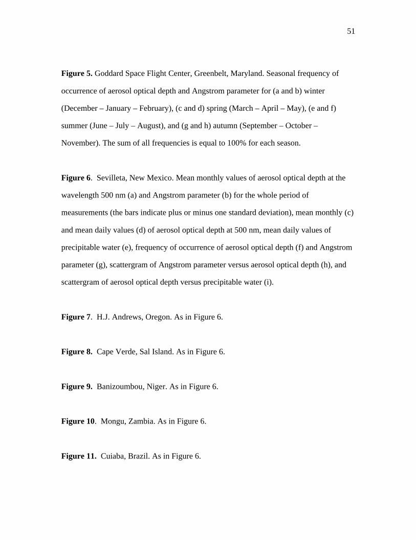
51

Figure 5. Goddard Space Flight Center, Greenbelt, Maryland. Seasonal frequency of

occurrence of aerosol optical depth and Angstrom parameter for (a and b) winter

(December – January – February), (c and d) spring (March – April – May), (e and f)

summer (June – July – August), and (g and h) autumn (September – October –

November). The sum of all frequencies is equal to 100% for each season.

Figure 6. Sevilleta, New Mexico. Mean monthly values of aerosol optical depth at the

wavelength 500 nm (a) and Angstrom parameter (b) for the whole period of

measurements (the bars indicate plus or minus one standard deviation), mean monthly (c)

and mean daily values (d) of aerosol optical depth at 500 nm, mean daily values of

precipitable water (e), frequency of occurrence of aerosol optical depth (f) and Angstrom

parameter (g), scattergram of Angstrom parameter versus aerosol optical depth (h), and

scattergram of aerosol optical depth versus precipitable water (i).

Figure 7. H.J. Andrews, Oregon. As in Figure 6.

Figure 8. Cape Verde, Sal Island. As in Figure 6.

Figure 9. Banizoumbou, Niger. As in Figure 6.

Figure 10. Mongu, Zambia. As in Figure 6.

Figure 11. Cuiaba, Brazil. As in Figure 6.

52

Figure 12. Thompson, Manitoba, Canada. As in Figure 6.

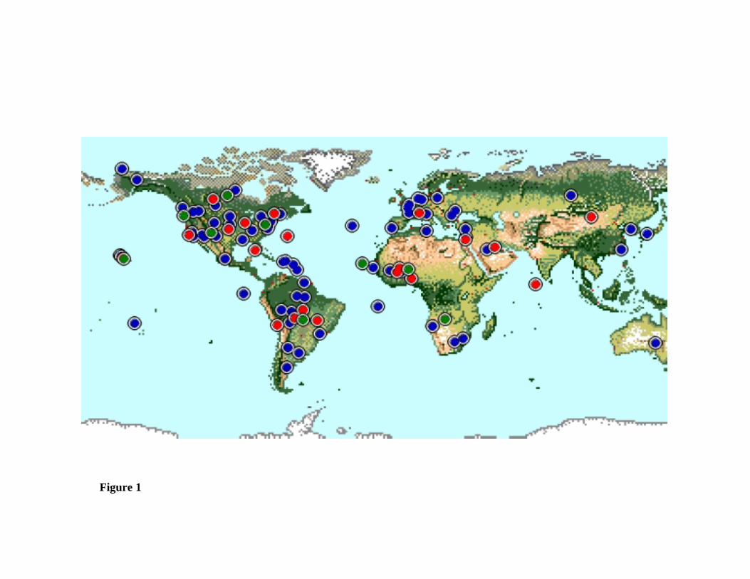
Figure 1

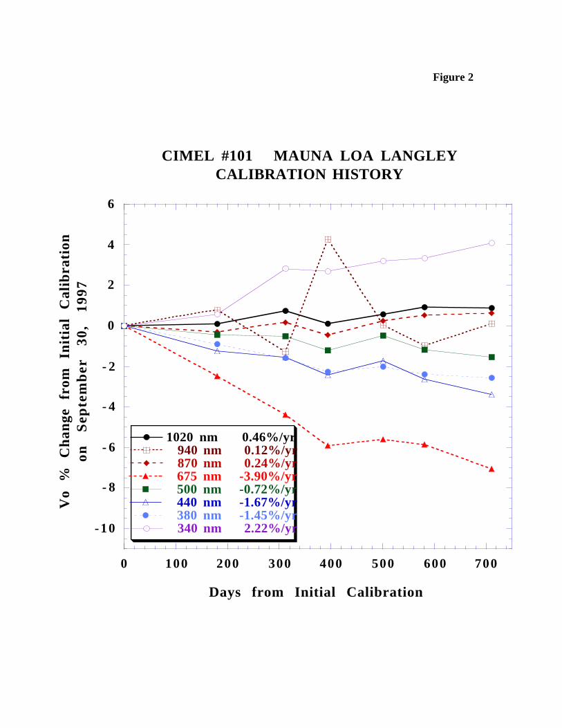
Figure 2

-10

- 8

- 6

- 4

- 2

0

2

4

6

0 100 200 300 400 500 600 700

CIMEL #101 MAUNA LOA LANGLEYCALIBRATION HISTORY

1020 nm 0.46%/yr 940 nm 0.12%/yr 870 nm 0.24%/yr 675 nm -3.90%/yr 500 nm -0.72%/yr 440 nm -1.67%/yr 380 nm -1.45%/yr 340 nm 2.22%/yr

Vo

%

Ch

ange

fr

om

Init

ial

Cal

ibra

tion

on

Sep

tem

ber

30

, 19

97

Days from Initial Calibration

Figure 3a)

b)

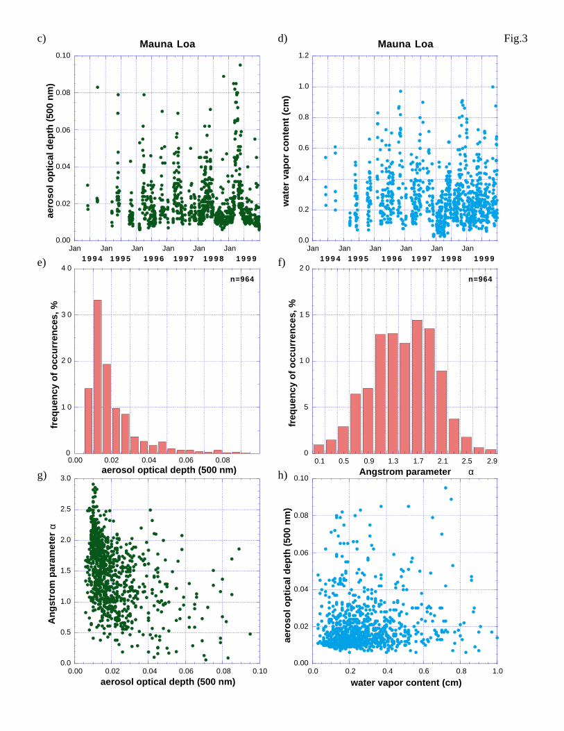
0.00

0.02

0.04

0.06

0.08

0.10

Jan Jan Jan Jan Jan Jan

Mauna Loaae

roso

l op

tica

l dep

th (

500

nm

)

1 9 9 4 1 9 9 5 1 9 9 6 1 9 9 7 1 9 9 8 1 9 9 9

0.0

0.2

0.4

0.6

0.8

1.0

1.2

Jan Jan Jan Jan Jan Jan

Mauna Loa

wat

er v

apo

r co

nte

nt

(cm

)

1 9 9 4 1 9 9 5 1 9 9 6 1 9 9 7 1 9 9 8 1 9 9 9

0

1 0

2 0

3 0

4 0

0.00 0.02 0.04 0.06 0.08

freq

uen

cy o

f o

ccu

rren

ces,

%

aerosol optical depth (500 nm)

n=964

0

5

1 0

1 5

2 0

0.1 0.5 0.9 1.3 1.7 2.1 2.5 2.9

freq

uen

cy o

f o

ccu

rren

ces,

%

Angstrom parameter α

n=964

0.0

0.5

1.0

1.5

2.0

2.5

3.0

0.00 0.02 0.04 0.06 0.08 0.10

An

gst

rom

par

amet

er α

aerosol optical depth (500 nm)

0.00

0.02

0.04

0.06

0.08

0.10

0.0 0.2 0.4 0.6 0.8 1.0

aero

sol o

pti

cal d

epth

(50

0 n

m)

water vapor content (cm)

Fig.3c) d)

e) f)

g) h)

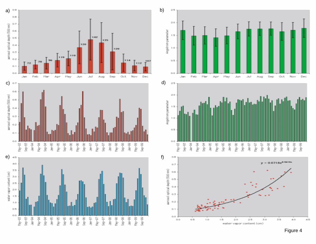
a) b)

c) d)

e) f)

Figure 4

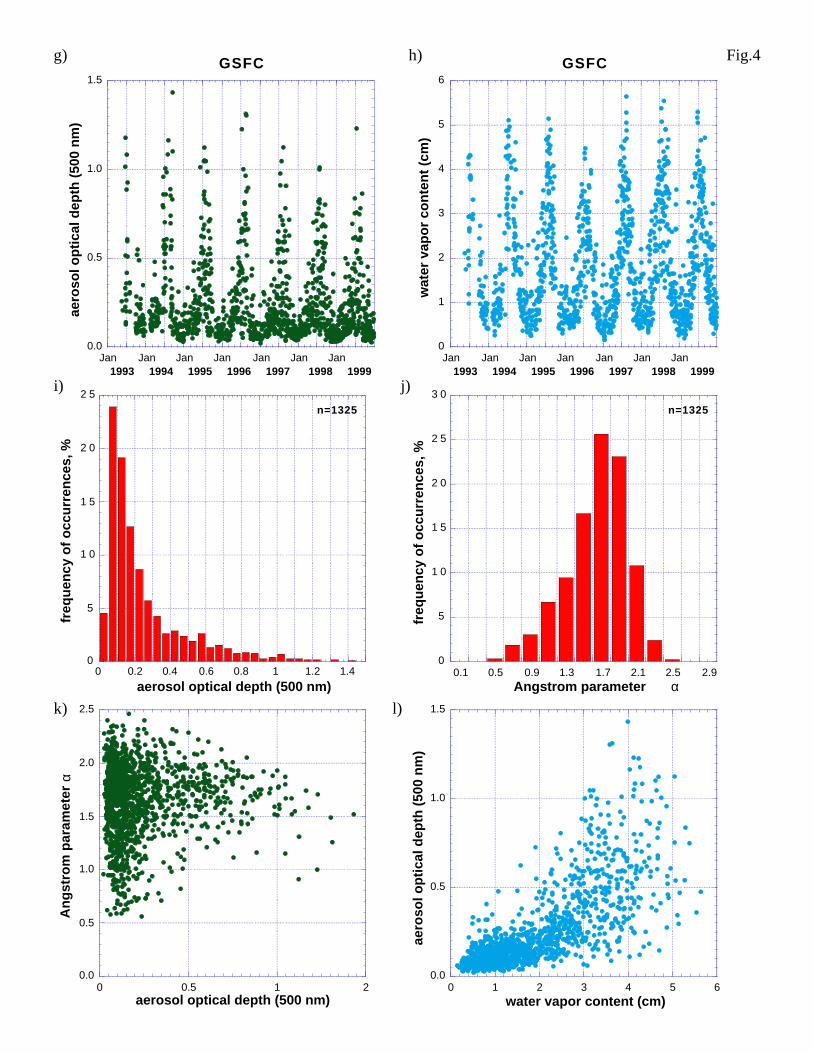
0.0

0.5

1.0

1.5

Jan Jan Jan Jan Jan Jan Jan

GSFCae

roso

l op

tica

l dep

th (

500

nm

)

1993 1994 1995 1996 1997 1998 1999

0

1

2

3

4

5

6

Jan Jan Jan Jan Jan Jan Jan

GSFC

wat

er v

apo

r co

nte

nt

(cm

)

1993 1994 1995 1996 1997 1998 1999

0.0

0.5

1.0

1.5

2.0

2.5

0 0.5 1 2

An

gst

rom

par

amet

er α

aerosol optical depth (500 nm)

0.0

0.5

1.0

1.5

0 1 2 3 4 5 6

aero

sol o

pti

cal d

epth

(50

0 n

m)

water vapor content (cm)

g) h)

i) j)

k) l)

Fig.4

0

5

1 0

1 5

2 0

2 5

0 0.2 0.4 0.6 0.8 1 1.2 1.4

freq

uen

cy o

f o

ccu

rren

ces,

%

aerosol optical depth (500 nm)

n=1325

0

5

1 0

1 5

2 0

2 5

3 0

0.1 0.5 0.9 1.3 1.7 2.1 2.5 2.9

freq

uen

cy o

f o

ccu

rren

ces,

%

Angstrom parameter α

n=1325

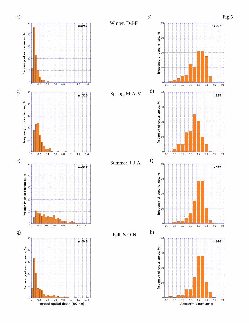
Fig.5Winter, D-J-F

Spring, M-A-M

Summer, J-J-A

Fall, S-O-N

a) b)

c) d)

e) f)

g) h)

0

10

20

30

40

50

0 0.2 0.4 0.6 0.8 1 1.2 1.4

freq

uen

cy o

f o

ccu

rren

ces,

%n=257

0

10

20

30

40

0.1 0.5 0.9 1.3 1.7 2.1 2.5 2.9

n=257

freq

uen

cy o

f o

ccu

rren

ces,

%

0

10

20

30

40

50

0 0.2 0.4 0.6 0.8 1 1.2 1.4

freq

uen

cy o

f o

ccu

rren

ces,

%

n=325

0

10

20

30

40

50

0 0.2 0.4 0.6 0.8 1 1.2 1.4

freq

uen

cy o

f o

ccu

rren

ces,

%

n=397

0

10

20

30

40

50

0 0.2 0.4 0.6 0.8 1 1.2 1.4

freq

uen

cy o

f o

ccu

rren

ces,

%

aerosol optical depth (500 nm)

n=346

0

10

20

30

40

0.1 0.5 0.9 1.3 1.7 2.1 2.5 2.9

Angstrom parameter α

freq

uen

cy o

f o

ccu

rren

ces,

%

n=346

0

10

20

30

40

0.1 0.5 0.9 1.3 1.7 2.1 2.5 2.9

freq

uen

cy o

f o

ccu

rren

ces,

%

n=397

0

10

20

30

40

0.1 0.5 0.9 1.3 1.7 2.1 2.5 2.9

n=325

freq

uen

cy o

f o

ccu

rren

ces,

%

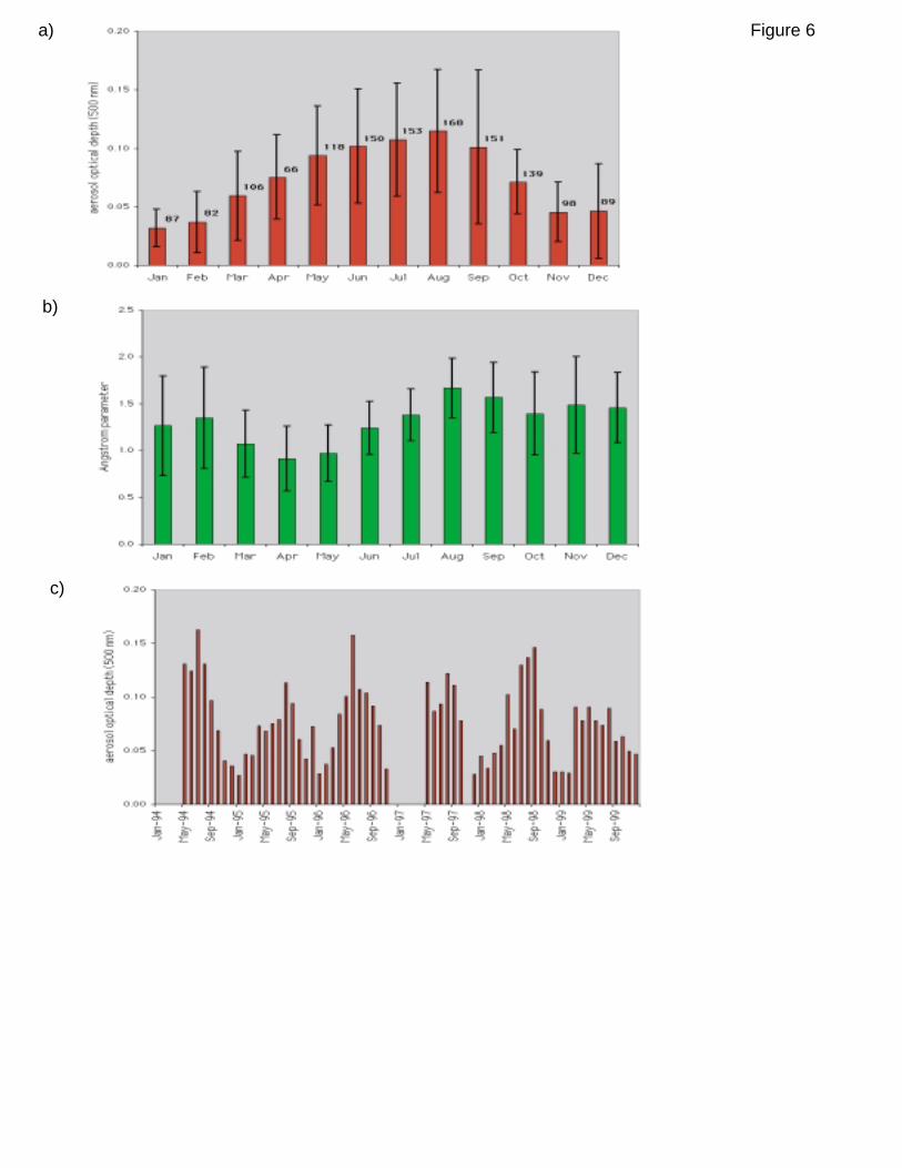
Figure 6a)

b)

c)

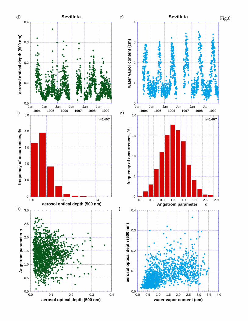
0.0

0.1

0.2

0.3

0.4

Jan Jan Jan Jan Jan Jan

Sevilletaae

roso

l op

tica

l dep

th (

500

nm

)

1994 1995 1996 1997 1998 1999

0

1

2

3

4

Jan Jan Jan Jan Jan Jan

Sevilleta

wat

er v

apo

r co

nte

nt

(cm

)

1994 1995 1996 1997 1998 1999

0

1 0

2 0

3 0

4 0

5 0

0.0 0.2 0.4

freq

uen

cy o

f o

ccu

rren

ces,

%

aerosol optical depth (500 nm)

n=1407

0

5

1 0

1 5

2 0

0.1 0.5 0.9 1.3 1.7 2.1 2.5 2.9

freq

uen

cy o

f o

ccu

rren

ces,

%

Angstrom parameter α

n=1407

0.0

0.5

1.0

1.5

2.0

2.5

3.0

0.0 0.1 0.2 0.3 0.4

An

gst

rom

par

amet

er α

aerosol optical depth (500 nm)

0.0

0.1

0.2

0.3

0.4

0.0 0.5 1.0 1.5 2.0 2.5 3.0 3.5 4.0

aero

sol o

pti

cal d

epth

(50

0 n

m)

water vapor content (cm)

Fig.6d) e)

f) g)

h) i)

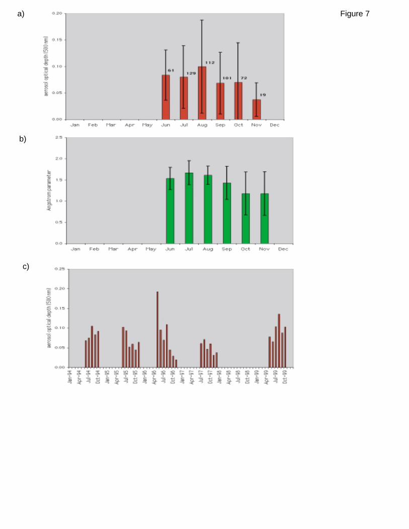
Figure 7a)

b)

c)

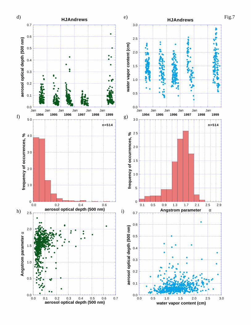
0.0

0.1

0.2

0.3

0.4

0.5

0.6

0.7

Jan Jan Jan Jan Jan Jan

HJAndrewsae

roso

l op

tica

l dep

th (

500

nm

)

1994 1995 1996 1997 1998 1999

0.0

0.5

1.0

1.5

2.0

2.5

3.0

Jan Jan Jan Jan Jan Jan

HJAndrews

wat

er v

apo

r co

nte

nt

(cm

)

1994 1995 1996 1997 1998 1999

0

1 0

2 0

3 0

4 0

5 0

0.0 0.2 0.4 0.6

freq

uen

cy o

f o

ccu

rren

ces,

%

aerosol optical depth (500 nm)

n=514

0

5

1 0

1 5

2 0

2 5

3 0

0.1 0.5 0.9 1.3 1.7 2.1 2.5 2.9

freq

uen

cy o

f o

ccu

rren

ces,

%

Angstrom parameter α

n=514

0.0

0.5

1.0

1.5

2.0

2.5

0.0 0.1 0.2 0.3 0.4 0.5 0.6 0.7

An

gst

rom

par

amet

er α

aerosol optical depth (500 nm)

0.0

0.1

0.2

0.3

0.4

0.5

0.6

0.7

0.0 0.5 1.0 1.5 2.0 2.5 3.0

aero

sol o

pti

cal d

epth

(50

0 n

m)

water vapor content (cm)

Fig.7d) e)

f) g)

h) i)

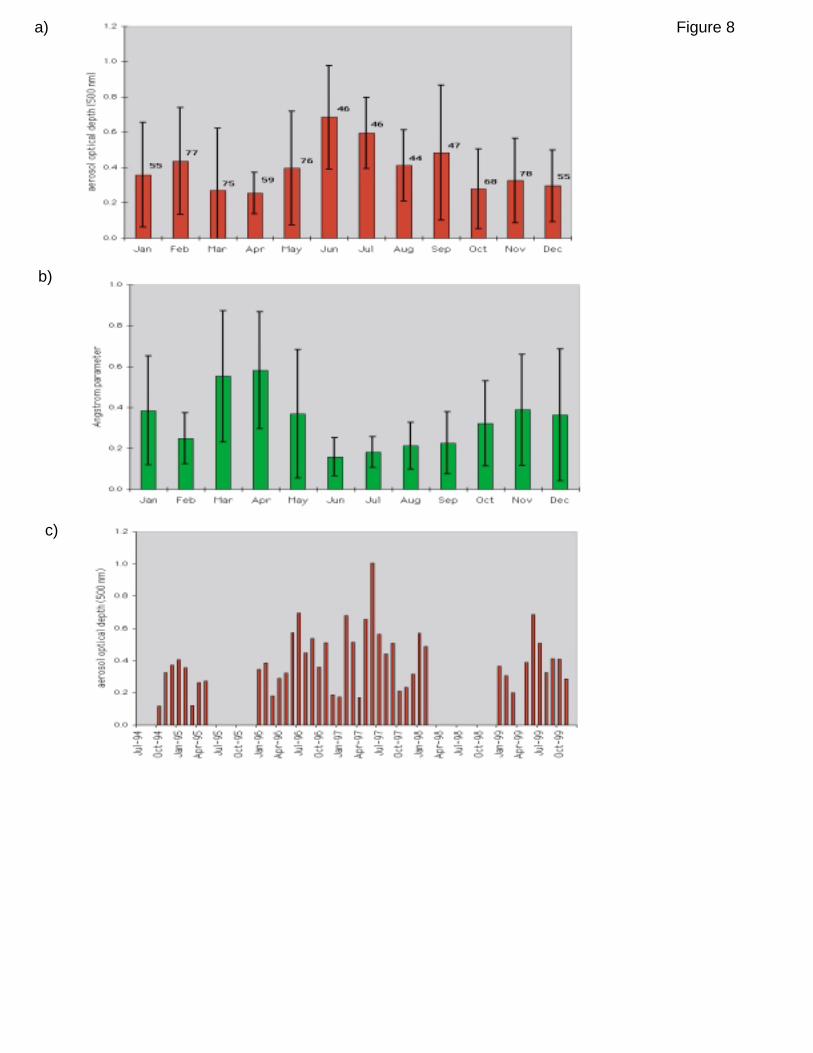
Figure 8a)

b)

c)

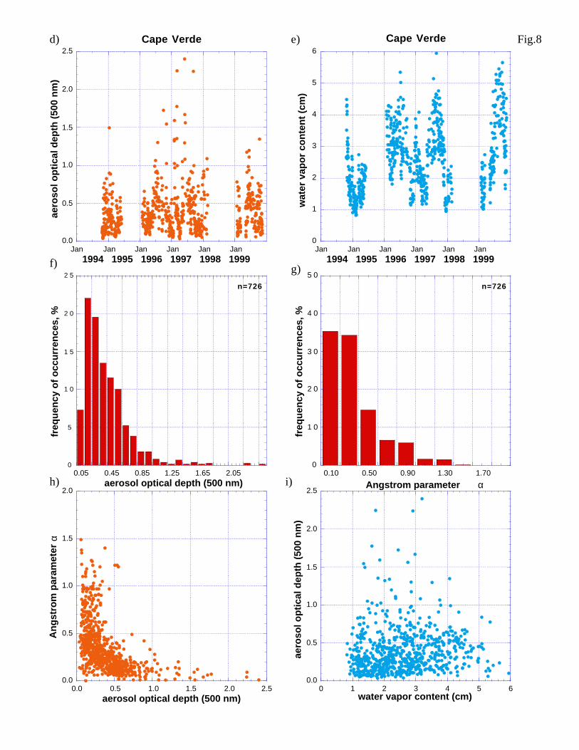
0.0

0.5

1.0

1.5

2.0

2.5

Jan Jan Jan Jan Jan Jan

Cape Verdeae

roso

l op

tica

l dep

th (

500

nm

)

1994 1995 1996 1997 1998 1999

0

1

2

3

4

5

6

Jan Jan Jan Jan Jan Jan

Cape Verde

wat

er v

apo

r co

nte

nt

(cm

)

1994 1995 1996 1997 1998 1999

0

5

1 0

1 5

2 0

2 5

0.05 0.45 0.85 1.25 1.65 2.05

freq

uen

cy o

f o

ccu

rren

ces,

%

aerosol optical depth (500 nm)

n=726

0

1 0

2 0

3 0

4 0

5 0

0.10 0.50 0.90 1.30 1.70

freq

uen

cy o

f o

ccu

rren

ces,

%

Angstrom parameter α

n=726

0.0

0.5

1.0

1.5

2.0

2.5

0 1 2 3 4 5 6

aero

sol o

pti

cal d

epth

(50

0 n

m)

water vapor content (cm)

0.0

0.5

1.0

1.5

2.0

0.0 0.5 1.0 1.5 2.0 2.5

An

gst

rom

par

amet

er α

aerosol optical depth (500 nm)

Fig.8d)

f)

h)

e)

g)

i)

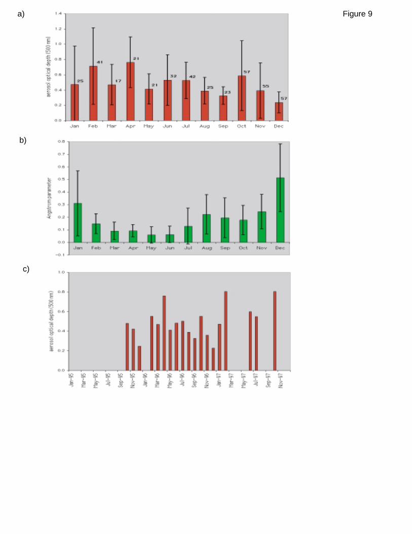
Figure 9a)

b)

c)

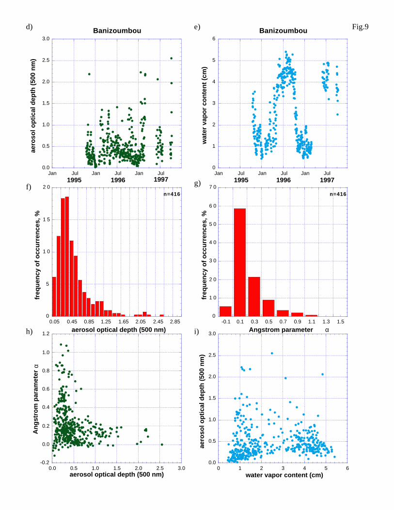
0.0

0.5

1.0

1.5

2.0

2.5

3.0

Jan Jul Jan Jul Jan Jul

Banizoumbouae

roso

l op

tica

l dep

th (

500

nm

)

1995 1996 1997

0

1

2

3

4

5

6

Jan Jul Jan Jul Jan Jul

Banizoumbou

wat

er v

apo

r co

nte

nt

(cm

)

1995 1996 1997

0

5

1 0

1 5

2 0

0.05 0.45 0.85 1.25 1.65 2.05 2.45 2.85

freq

uen

cy o

f o

ccu

rren

ces,

%

aerosol optical depth (500 nm)

n=416

0

1 0

2 0

3 0

4 0

5 0

6 0

7 0

-0.1 0.1 0.3 0.5 0.7 0.9 1.1 1.3 1.5

freq

uen

cy o

f o

ccu

rren

ces,

%

Angstrom parameter α

n=416

-0.2

0.0

0.2

0.4

0.6

0.8

1.0

1.2

0.0 0.5 1.0 1.5 2.0 2.5 3.0

An

gst

rom

par

amet

er α

aerosol optical depth (500 nm)

0.0

0.5

1.0

1.5

2.0

2.5

3.0

0 1 2 3 4 5 6

aero

sol o

pti

cal d

epth

(50

0 n

m)

water vapor content (cm)

d)

f)

h)

e)

g)

i)

Fig.9

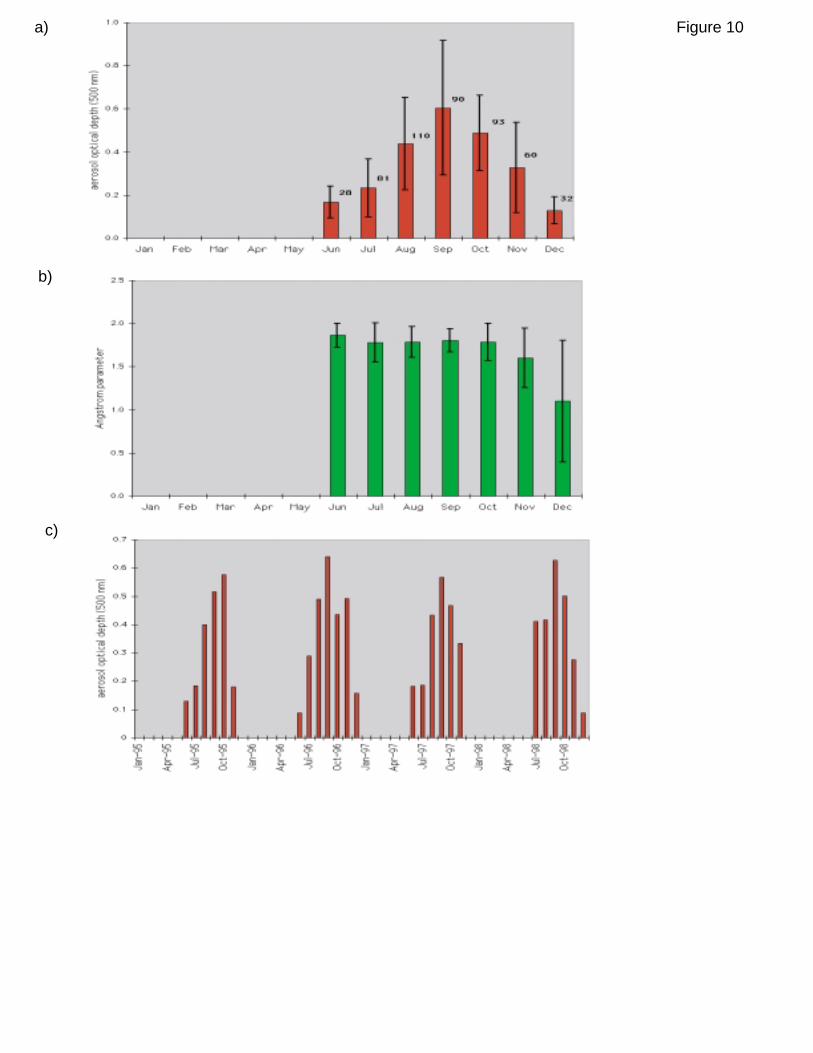
Figure 10a)

b)

c)

0.0

0.5

1.0

1.5

2.0

2.5

0.0 0.5 1.0 1.5 2.0

An

gst

rom

par

amet

er α

aerosol optical depth (500 nm)

0.0

0.5

1.0

1.5

2.0

0 1 2 3 4 5

aero

sol o

pti

cal d

epth

(50

0 n

m)

water vapor content (cm)

0

5

1 0

1 5

2 0

0.05 0.25 0.45 0.65 0.85 1.05 1.25 1.45 1.65

freq

uen

cy o

f o

ccu

rren

ces,

%

aerosol optical depth (500 nm)

n=493

0

1 0

2 0

3 0

4 0

5 0

0.1 0.5 0.9 1.3 1.7 2.1 2.5 2.9

freq

uen

cy o

f o

ccu

rren

ces,

%

Angstrom parameter α

n=493

0.0

0.5

1.0

1.5

2.0

Jan Jul Jan Jul Jan Jul Jan Jul

Monguae

roso

l op

tica

l dep

th (

500

nm

)

1995 1996 1997 1998

0

1

2

3

4

5

Jan Jul Jan Jul Jan Jul Jan Jul

Mongu

wat

er v

apo

r co

nte

nt

(cm

)

1995 1996 1997 1998

d) e)

f) g)

h) i)

Fig.10

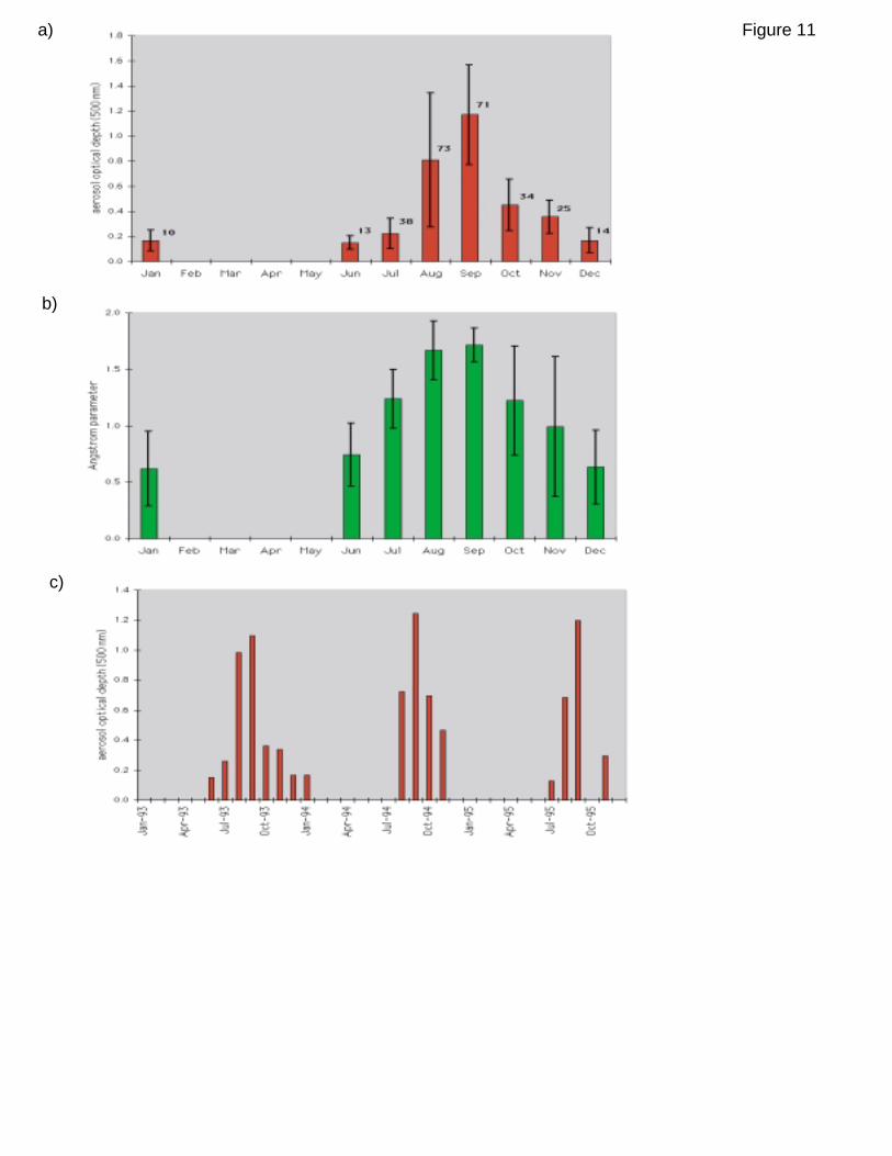
Figure 11a)

b)

c)

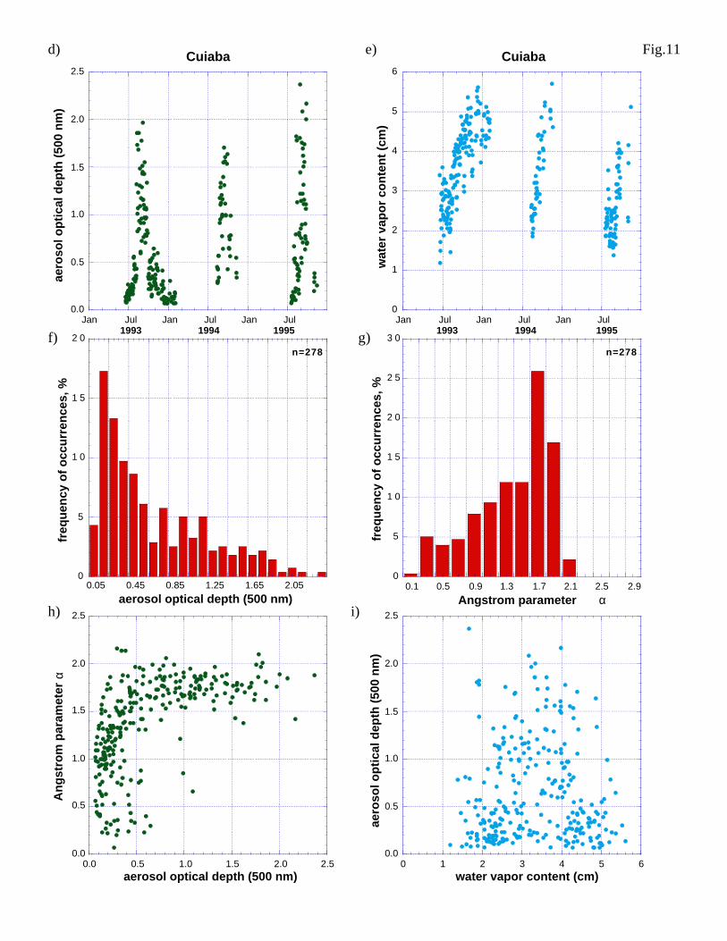
0.0

0.5

1.0

1.5

2.0

2.5

Jan Jul Jan Jul Jan Jul

Cuiabaae

roso

l op

tica

l dep

th (

500

nm

)

1993 1994 1995

0

1

2

3

4

5

6

Jan Jul Jan Jul Jan Jul

Cuiaba

wat

er v

apo

r co

nte

nt

(cm

)

1993 1994 1995

0

5

1 0

1 5

2 0

0.05 0.45 0.85 1.25 1.65 2.05

n=278

aerosol optical depth (500 nm)

freq

uen

cy o

f o

ccu

rren

ces,

%

0

5

1 0

1 5

2 0

2 5

3 0

0.1 0.5 0.9 1.3 1.7 2.1 2.5 2.9

n=278

Angstrom parameter α

freq

uen

cy o

f o

ccu

rren

ces,

%

0.0

0.5

1.0

1.5

2.0

2.5

0.0 0.5 1.0 1.5 2.0 2.5

An

gst

rom

par

amet

er α

aerosol optical depth (500 nm)

0.0

0.5

1.0

1.5

2.0

2.5

0 1 2 3 4 5 6

aero

sol o

pti

cal d

epth

(50

0 n

m)

water vapor content (cm)

d) e)

f) g)

h) i)

Fig.11

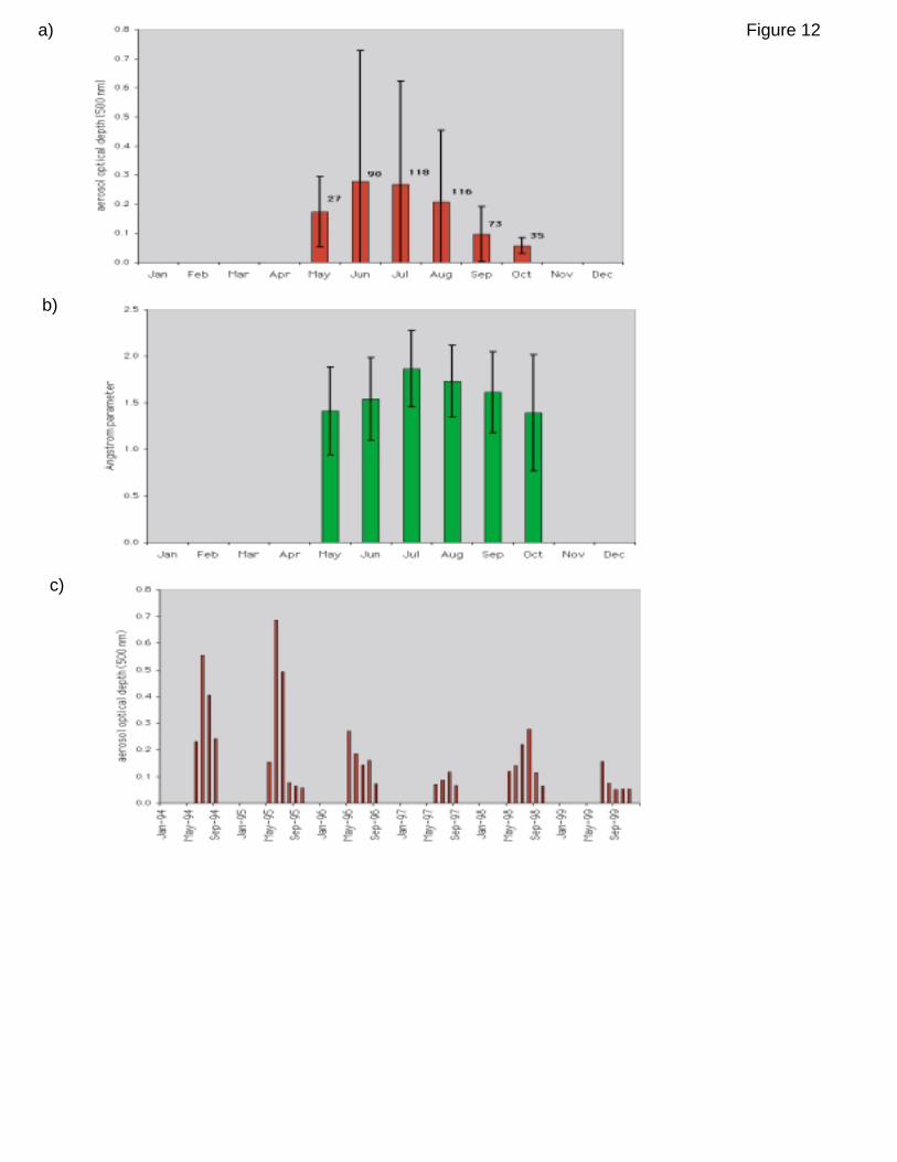
Figure 12a)

b)

c)

0.0

0.5

1.0

1.5

2.0

2.5

3.0

3.5

Jan Jan Jan Jan Jan Jan

Thompsonae

roso

l op

tica

l dep

th (

500

nm

)

1994 1995 1996 1997 1998 1999

0.0

0.5

1.0

1.5

2.0

2.5

3.0

3.5

4.0

Jan Jan Jan Jan Jan Jan

Thompson

wat

er v

apo

r co

nte

nt

(cm

)

1994 1995 1996 1997 1998 1999

0.0

0.5

1.0

1.5

2.0

2.5

3.0

0 0.5 1 1.5 2 2.5 3 3.5

An

gst

rom

par

amet

er α

aerosol optical depth (500 nm)

0.0

0.5

1.0

1.5

2.0

2.5

3.0

3.5

0.0 0.5 1.0 1.5 2.0 2.5 3.0 3.5 4.0

aero

sol o

pti

cal d

epth

(50

0 n

m)

water vapor content (cm)

0

5

1 0

1 5

2 0

2 5

3 0

0.1 0.5 0.9 1.3 1.7 2.1

freq

uen

cy o

f o

ccu

rren

ces,

%

aerosol optical depth (500 nm)

n=459

0

5

1 0

1 5

2 0

2 5

0.1 0.5 0.9 1.3 1.7 2.1 2.5 2.9

freq

uen

c o

f o

ccu

rren

ces,

%

Angstrom parameter α

n=459

d) e)

f) g)

h) i)

Fig.12

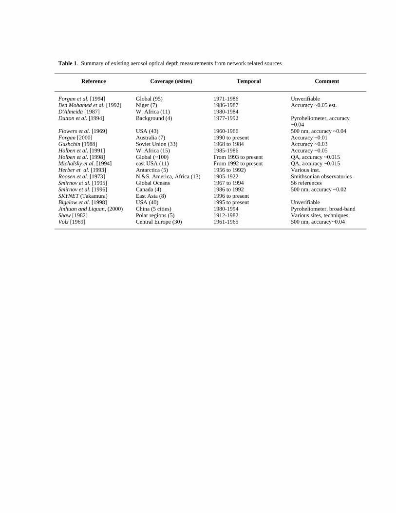
Table 1. Summary of existing aerosol optical depth measurements from network related sources

Reference Coverage (#sites) Temporal Comment

Forgan et al. [1994] Global (95) 1971-1986 UnverifiableBen Mohamed et al. [1992] Niger (7) 1986-1987 Accuracy ~0.05 est.D'Almeida [1987] W. Africa (11) 1980-1984Dutton et al. [1994] Background (4) 1977-1992 Pyroheliometer, accuracy

~0.04Flowers et al. [1969] USA (43) 1960-1966 500 nm, accuracy ~0.04Forgan [2000] Australia (7) 1990 to present Accuracy ~0.01Gushchin [1988] Soviet Union (33) 1968 to 1984 Accuracy ~0.03Holben et al. [1991] W. Africa (15) 1985-1986 Accuracy ~0.05Holben et al. [1998] Global (~100) From 1993 to present QA, accuracy ~0.015Michalsky et al. [1994] east USA (11) From 1992 to present QA, accuracy ~0.015Herber et al. [1993] Antarctica (5) 1956 to 1992) Various inst.Roosen et al. [1973] N &S. America, Africa (13) 1905-1922 Smithsonian observatoriesSmirnov et al. [1995] Global Oceans 1967 to 1994 56 referencesSmirnov et al. [1996] Canada (4) 1986 to 1992 500 nm, accuracy ~0.02SKYNET (Takamura) East Asia (8) 1996 to presentBigelow et al. [1998] USA (40) 1995 to present UnverifiableJinhuan and Liquan, (2000) China (5 cities) 1980-1994 Pyroheliometer, broad-bandShaw [1982] Polar regions (5) 1912-1982 Various sites, techniquesVolz [1969] Central Europe (30) 1961-1965 500 nm, accuracy~0.04

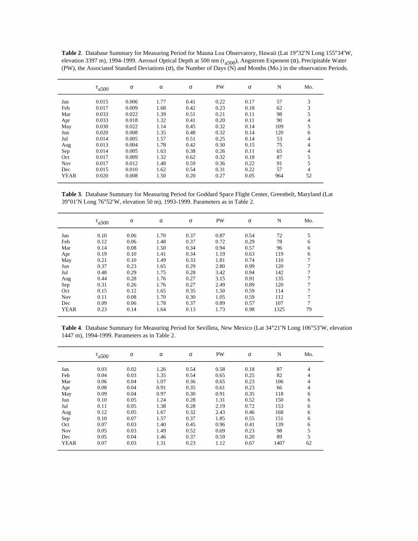
Table 2. Database Summary for Measuring Period for Mauna Loa Observatory, Hawaii (Lat 19°32′N Long 155°34′W,elevation 3397 m), 1994-1999. Aerosol Optical Depth at 500 nm (τa500), Angstrom Expenent (α), Precipitable Water(PW), the Associated Standard Deviations (σ), the Number of Days (N) and Months (Mo.) in the observation Periods.

τa500 σ α σ PW σ N Mo.

Jan 0.015 0.006 1.77 0.41 0.22 0.17 57 3Feb 0.017 0.009 1.68 0.42 0.23 0.18 62 3Mar 0.033 0.022 1.39 0.51 0.21 0.11 98 5Apr 0.033 0.018 1.32 0.41 0.20 0.11 90 4May 0.030 0.022 1.14 0.45 0.32 0.14 109 5Jun 0.020 0.008 1.35 0.48 0.32 0.14 120 6Jul 0.014 0.005 1.57 0.51 0.25 0.14 53 4Aug 0.013 0.004 1.78 0.42 0.30 0.15 75 4Sep 0.014 0.005 1.63 0.38 0.26 0.11 65 4Oct 0.017 0.009 1.32 0.62 0.32 0.18 87 5Nov 0.017 0.012 1.48 0.59 0.36 0.22 91 5Dec 0.015 0.010 1.62 0.54 0.31 0.22 57 4YEAR 0.020 0.008 1.50 0.20 0.27 0.05 964 52

Table 3. Database Summary for Measuring Period for Goddard Space Flight Center, Greenbelt, Maryland (Lat39°01′N Long 76°52′W, elevation 50 m), 1993-1999. Parameters as in Table 2.

τa500 σ α σ PW σ N Mo.

Jan 0.10 0.06 1.70 0.37 0.87 0.54 72 5Feb 0.12 0.06 1.48 0.37 0.72 0.29 78 6Mar 0.14 0.08 1.50 0.34 0.94 0.57 96 6Apr 0.19 0.10 1.41 0.34 1.19 0.63 119 6May 0.21 0.10 1.49 0.33 1.81 0.74 110 7Jun 0.37 0.23 1.65 0.29 2.80 0.99 120 7Jul 0.48 0.29 1.75 0.28 3.42 0.94 142 7Aug 0.44 0.28 1.76 0.27 3.15 0.91 135 7Sep 0.31 0.26 1.76 0.27 2.49 0.89 120 7Oct 0.15 0.12 1.65 0.35 1.50 0.59 114 7Nov 0.11 0.08 1.70 0.30 1.05 0.59 112 7Dec 0.09 0.06 1.78 0.37 0.89 0.57 107 7YEAR 0.23 0.14 1.64 0.13 1.73 0.98 1325 79

Table 4. Database Summary for Measuring Period for Sevilleta, New Mexico (Lat 34°21′N Long 106°53′W, elevation1447 m), 1994-1999. Parameters as in Table 2.

τa500 σ α σ PW σ N Mo.

Jan 0.03 0.02 1.26 0.54 0.58 0.18 87 4Feb 0.04 0.03 1.35 0.54 0.65 0.25 82 4Mar 0.06 0.04 1.07 0.36 0.65 0.23 106 4Apr 0.08 0.04 0.91 0.35 0.61 0.23 66 4May 0.09 0.04 0.97 0.30 0.91 0.35 118 6Jun 0.10 0.05 1.24 0.28 1.31 0.52 150 6Jul 0.11 0.05 1.38 0.28 2.19 0.72 153 6Aug 0.12 0.05 1.67 0.32 2.43 0.46 168 6Sep 0.10 0.07 1.57 0.37 1.85 0.55 151 6Oct 0.07 0.03 1.40 0.45 0.96 0.41 139 6Nov 0.05 0.03 1.49 0.52 0.69 0.23 98 5Dec 0.05 0.04 1.46 0.37 0.59 0.20 89 5YEAR 0.07 0.03 1.31 0.23 1.12 0.67 1407 62

Table 5. Database Summary for Measuring Period for HJAndrews, Oregon (Lat 44°14′N Long 122°13′W, elevation

830 m), 1994-1999. Parameters as in Table 2.

τa500 σ α σ PW σ N Mo.

Jan ... ... ... ... ... ... ... …Feb ... ... ... ... ... ... ... …Mar ... ... ... ... ... ... ... …Apr ... ... ... ... ... ... ... …May 0.15 0.09 1.52 0.26 1.12 0.34 10 2Jun 0.08 0.05 1.53 0.26 1.41 0.43 61 4Jul 0.08 0.06 1.67 0.28 1.61 0.39 129 5Aug 0.10 0.09 1.61 0.22 1.65 0.50 112 5Sep 0.07 0.06 1.43 0.39 1.32 0.33 101 5Oct 0.07 0.07 1.18 0.51 1.07 0.35 72 5Nov 0.04 0.03 1.18 0.52 0.89 0.35 19 3Dec 0.04 0.02 0.74 0.52 0.82 0.32 10 1YEAR ... ... ... ... ... ... 514 30

Table 6. Database Summary for Cape Verde (Lat 16°43′N Long 22°56′W, elevation 60 m), 1994-1999. Parameters as

in Table 2.

τa500 σ α σ PW σ N Mo.

Jan 0.36 0.30 0.39 0.27 1.96 0.83 55 5Feb 0.44 0.30 0.25 0.12 1.93 0.90 77 5Mar 0.27 0.35 0.55 0.32 2.09 0.70 75 4Apr 0.26 0.12 0.58 0.29 2.21 0.79 59 3May 0.40 0.32 0.37 0.31 2.39 0.72 76 4Jun 0.68 0.29 0.16 0.09 3.10 0.71 46 3Jul 0.60 0.20 0.18 0.08 3.53 0.93 46 3Aug 0.41 0.20 0.21 0.11 3.90 0.89 44 3Sep 0.48 0.38 0.23 0.15 3.70 0.83 47 3Oct 0.28 0.23 0.32 0.21 3.33 0.80 68 4Nov 0.33 0.24 0.39 0.27 2.39 0.74 78 4Dec 0.30 0.20 0.36 0.32 1.81 0.67 55 3YEAR 0.40 0.13 0.33 0.14 2.69 0.76 726 44

Table 7. Database Summary for Banizoumbou, Niger (Lat 32°22′N Long 02°39′E, elevation 250 m), 1995-1997.

Parameters as in Table 2.

τa500 σ α σ PW σ N Mo.

Jan 0.47 0.50 0.31 0.26 1.15 0.48 25 1Feb 0.71 0.50 0.15 0.08 0.96 0.19 41 2Mar 0.47 0.26 0.09 0.07 1.64 0.60 17 1Apr 0.76 0.33 0.09 0.05 2.22 0.90 21 1May 0.41 0.20 0.06 0.07 3.34 1.03 21 1Jun 0.53 0.33 0.06 0.07 4.19 0.37 32 2Jul 0.52 0.24 0.13 0.14 4.30 0.47 42 2Aug 0.39 0.18 0.22 0.16 4.68 0.38 25 1Sep 0.33 0.12 0.20 0.16 4.38 0.33 23 1Oct 0.59 0.46 0.18 0.12 2.87 0.94 57 3Nov 0.39 0.36 0.25 0.14 1.24 0.52 55 2Dec 0.24 0.14 0.51 0.27 1.24 0.43 57 2YEAR 0.48 0.15 0.19 0.13 2.68 1.45 416 19

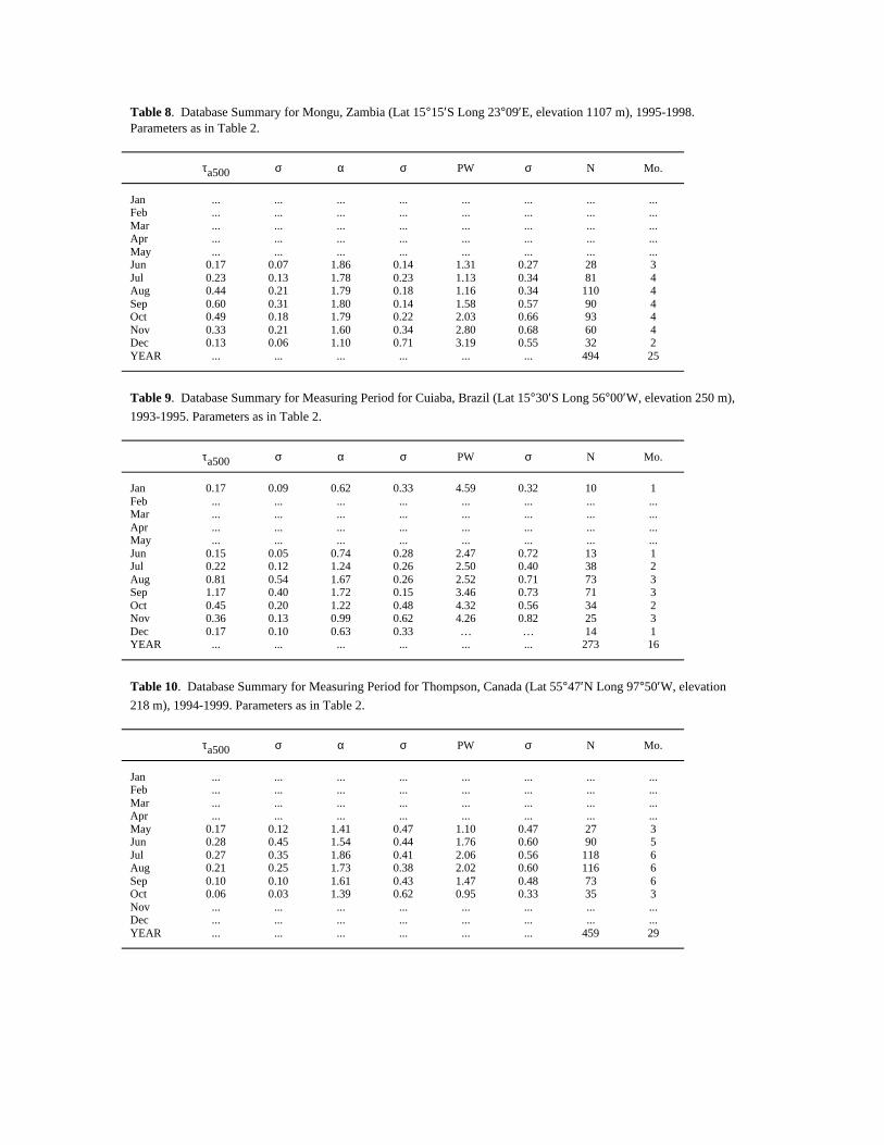
Table 8. Database Summary for Mongu, Zambia (Lat 15°15′S Long 23°09′E, elevation 1107 m), 1995-1998.Parameters as in Table 2.

τa500 σ α σ PW σ N Mo.

Jan ... ... ... ... ... ... ... ...Feb ... ... ... ... ... ... ... ...Mar ... ... ... ... ... ... ... ...Apr ... ... ... ... ... ... ... ...May ... ... ... ... ... ... ... ...Jun 0.17 0.07 1.86 0.14 1.31 0.27 28 3Jul 0.23 0.13 1.78 0.23 1.13 0.34 81 4Aug 0.44 0.21 1.79 0.18 1.16 0.34 110 4Sep 0.60 0.31 1.80 0.14 1.58 0.57 90 4Oct 0.49 0.18 1.79 0.22 2.03 0.66 93 4Nov 0.33 0.21 1.60 0.34 2.80 0.68 60 4Dec 0.13 0.06 1.10 0.71 3.19 0.55 32 2YEAR ... ... ... ... ... ... 494 25

Table 9. Database Summary for Measuring Period for Cuiaba, Brazil (Lat 15°30′S Long 56°00′W, elevation 250 m),

1993-1995. Parameters as in Table 2.

τa500 σ α σ PW σ N Mo.

Jan 0.17 0.09 0.62 0.33 4.59 0.32 10 1Feb ... ... ... ... ... ... ... ...Mar ... ... ... ... ... ... ... ...Apr ... ... ... ... ... ... ... ...May ... ... ... ... ... ... ... ...Jun 0.15 0.05 0.74 0.28 2.47 0.72 13 1Jul 0.22 0.12 1.24 0.26 2.50 0.40 38 2Aug 0.81 0.54 1.67 0.26 2.52 0.71 73 3Sep 1.17 0.40 1.72 0.15 3.46 0.73 71 3Oct 0.45 0.20 1.22 0.48 4.32 0.56 34 2Nov 0.36 0.13 0.99 0.62 4.26 0.82 25 3Dec 0.17 0.10 0.63 0.33 … … 14 1YEAR ... ... ... ... ... ... 273 16

Table 10. Database Summary for Measuring Period for Thompson, Canada (Lat 55°47′N Long 97°50′W, elevation

218 m), 1994-1999. Parameters as in Table 2.

τa500 σ α σ PW σ N Mo.

Jan ... ... ... ... ... ... ... ...Feb ... ... ... ... ... ... ... ...Mar ... ... ... ... ... ... ... ...Apr ... ... ... ... ... ... ... ...May 0.17 0.12 1.41 0.47 1.10 0.47 27 3Jun 0.28 0.45 1.54 0.44 1.76 0.60 90 5Jul 0.27 0.35 1.86 0.41 2.06 0.56 118 6Aug 0.21 0.25 1.73 0.38 2.02 0.60 116 6Sep 0.10 0.10 1.61 0.43 1.47 0.48 73 6Oct 0.06 0.03 1.39 0.62 0.95 0.33 35 3Nov ... ... ... ... ... ... ... ...Dec ... ... ... ... ... ... ... ...YEAR ... ... ... ... ... ... 459 29

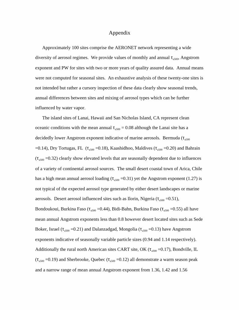
Appendix

Approximately 100 sites comprise the AERONET network representing a wide

diversity of aerosol regimes. We provide values of monthly and annual τa500, Angstrom

exponent and PW for sites with two or more years of quality assured data. Annual means

were not computed for seasonal sites. An exhaustive analysis of these twenty-one sites is

not intended but rather a cursory inspection of these data clearly show seasonal trends,

annual differences between sites and mixing of aerosol types which can be further

influenced by water vapor.

The island sites of Lanai, Hawaii and San Nicholas Island, CA represent clean

oceanic conditions with the mean annual τa500 = 0.08 although the Lanai site has a

decidedly lower Angstrom exponent indicative of marine aerosols. Bermuda (τa500

=0.14), Dry Tortugas, FL (τa500 =0.18), Kaashidhoo, Maldives (τa500 =0.20) and Bahrain

(τa500 =0.32) clearly show elevated levels that are seasonally dependent due to influences

of a variety of continental aerosol sources. The small desert coastal town of Arica, Chile

has a high mean annual aerosol loading (τa500 =0.31) yet the Angstrom exponent (1.27) is

not typical of the expected aerosol type generated by either desert landscapes or marine

aerosols. Desert aerosol influenced sites such as Ilorin, Nigeria (τa500 =0.51),

Bondoukoui, Burkina Faso (τa500 =0.44), Bidi-Bahn, Burkina Faso (τa500 =0.55) all have

mean annual Angstrom exponents less than 0.8 however desert located sites such as Sede

Boker, Israel (τa500 =0.21) and Dalanzadgad, Mongolia (τa500 =0.13) have Angstrom

exponents indicative of seasonally variable particle sizes (0.94 and 1.14 respectively).

Additionally the rural north American sites CART site, OK (τa500 =0.17), Bondville, IL

(τa500 =0.19) and Sherbrooke, Quebec (τa500 =0.12) all demonstrate a warm season peak

and a narrow range of mean annual Angstrom exponent from 1.36, 1.42 and 1.56

respectively. Ispra, Italy (0.36) is influenced by a rather constant aerosol source year

around as shown by high τa500 each month and a small range in angstrom exponent for all

months (mean α = 1.52). Lastly the seasonal values from the forested boreal site,

Waskesiu, Saskatchewan (τa500 =0.23, α = 1.41) and tropical forested sites, Alta Floresta

(τa500 =1.48, α = 1.66), Brazil and Brasilia, Brazil (τa500 = 0.56, α = 1.44) clearly respond

to the warm/dry season influence of biomass burning as described in detail earlier.

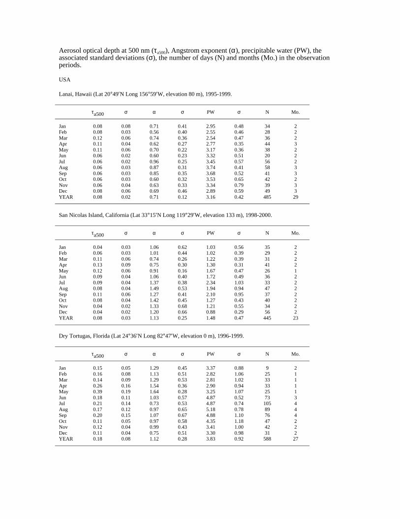
Aerosol optical depth at 500 nm (τa500), Angstrom exponent (α), precipitable water (PW), theassociated standard deviations (σ), the number of days (N) and months (Mo.) in the observationperiods.

USA

Lanai, Hawaii (Lat 20°49′N Long 156°59′W, elevation 80 m), 1995-1999.

τa500 σ α σ PW σ N Mo.

Jan 0.08 0.08 0.71 0.41 2.95 0.48 34 2Feb 0.08 0.03 0.56 0.40 2.55 0.46 28 2Mar 0.12 0.06 0.74 0.36 2.54 0.47 36 2Apr 0.11 0.04 0.62 0.27 2.77 0.35 44 3May 0.11 0.06 0.70 0.22 3.17 0.36 38 2Jun 0.06 0.02 0.60 0.23 3.32 0.51 20 2Jul 0.06 0.02 0.96 0.25 3.45 0.57 56 2Aug 0.06 0.03 0.87 0.31 3.74 0.41 58 3Sep 0.06 0.03 0.85 0.35 3.68 0.52 41 3Oct 0.06 0.03 0.60 0.32 3.53 0.65 42 2Nov 0.06 0.04 0.63 0.33 3.34 0.79 39 3Dec 0.08 0.06 0.69 0.46 2.89 0.59 49 3YEAR 0.08 0.02 0.71 0.12 3.16 0.42 485 29

San Nicolas Island, California (Lat 33°15′N Long 119°29′W, elevation 133 m), 1998-2000.

τa500 σ α σ PW σ N Mo.

Jan 0.04 0.03 1.06 0.62 1.03 0.56 35 2Feb 0.06 0.03 1.01 0.44 1.02 0.39 29 2Mar 0.11 0.06 0.74 0.26 1.22 0.39 31 2Apr 0.13 0.09 0.75 0.30 1.30 0.31 41 2May 0.12 0.06 0.91 0.16 1.67 0.47 26 1Jun 0.09 0.04 1.06 0.40 1.72 0.49 36 2Jul 0.09 0.04 1.37 0.38 2.34 1.03 33 2Aug 0.08 0.04 1.49 0.53 1.94 0.94 47 2Sep 0.11 0.06 1.27 0.41 2.10 0.95 37 2Oct 0.08 0.04 1.42 0.45 1.27 0.43 40 2Nov 0.04 0.02 1.33 0.68 1.21 0.55 34 2Dec 0.04 0.02 1.20 0.66 0.88 0.29 56 2YEAR 0.08 0.03 1.13 0.25 1.48 0.47 445 23

Dry Tortugas, Florida (Lat 24°36′N Long 82°47′W, elevation 0 m), 1996-1999.

τa500 σ α σ PW σ N Mo.

Jan 0.15 0.05 1.29 0.45 3.37 0.88 9 2Feb 0.16 0.08 1.13 0.51 2.82 1.06 25 1Mar 0.14 0.09 1.29 0.53 2.81 1.02 33 1Apr 0.26 0.16 1.54 0.36 2.90 0.94 33 1May 0.39 0.19 1.64 0.28 3.25 1.07 25 1Jun 0.18 0.11 1.03 0.57 4.87 0.52 73 3Jul 0.21 0.14 0.73 0.53 4.87 0.74 105 4Aug 0.17 0.12 0.97 0.65 5.18 0.78 89 4Sep 0.20 0.15 1.07 0.67 4.88 1.10 76 4Oct 0.11 0.05 0.97 0.58 4.35 1.18 47 2Nov 0.12 0.04 0.99 0.43 3.41 1.00 42 2Dec 0.11 0.04 0.75 0.51 3.30 0.98 31 2YEAR 0.18 0.08 1.12 0.28 3.83 0.92 588 27

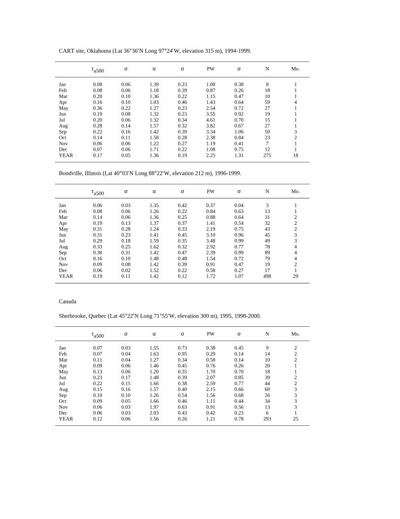
CART site, Oklahoma (Lat 36°36′N Long 97°24′W, elevation 315 m), 1994-1999.

τa500 σ α σ PW σ N Mo.

Jan 0.08 0.06 1.39 0.23 1.00 0.38 8 1Feb 0.08 0.06 1.18 0.39 0.87 0.26 18 1Mar 0.20 0.10 1.36 0.22 1.15 0.47 10 1Apr 0.16 0.10 1.03 0.46 1.43 0.64 59 4May 0.36 0.22 1.27 0.23 2.54 0.72 27 1Jun 0.19 0.08 1.32 0.23 3.55 0.92 19 1Jul 0.20 0.06 1.32 0.34 4.61 0.70 15 1Aug 0.28 0.14 1.57 0.32 3.82 0.67 27 1Sep 0.22 0.16 1.42 0.39 3.34 1.06 50 3Oct 0.14 0.11 1.58 0.28 2.38 0.84 23 2Nov 0.06 0.06 1.22 0.27 1.19 0.41 7 1Dec 0.07 0.06 1.71 0.22 1.08 0.75 12 1YEAR 0.17 0.05 1.36 0.19 2.25 1.31 275 18

Bondville, Illinois (Lat 40°03′N Long 88°22′W, elevation 212 m), 1996-1999.

τa500 σ α σ PW σ N Mo.

Jan 0.06 0.03 1.35 0.42 0.37 0.04 3 1Feb 0.08 0.06 1.26 0.22 0.84 0.63 13 1Mar 0.14 0.06 1.36 0.25 0.88 0.64 31 2Apr 0.19 0.13 1.37 0.37 1.41 0.54 32 2May 0.31 0.28 1.24 0.33 2.19 0.75 43 2Jun 0.31 0.23 1.41 0.45 3.10 0.96 45 3Jul 0.29 0.18 1.59 0.35 3.48 0.99 49 3Aug 0.33 0.25 1.62 0.32 2.92 0.77 78 4Sep 0.30 0.31 1.42 0.47 2.39 0.99 89 4Oct 0.16 0.10 1.48 0.48 1.54 0.72 79 4Nov 0.09 0.08 1.42 0.39 0.91 0.47 19 2Dec 0.06 0.02 1.52 0.22 0.58 0.27 17 1YEAR 0.19 0.11 1.42 0.12 1.72 1.07 498 29

Canada

Sherbrooke, Quebec (Lat 45°22′N Long 71°55′W, elevation 300 m), 1995, 1998-2000.

τa500 σ α σ PW σ N Mo.

Jan 0.07 0.03 1.55 0.73 0.38 0.45 9 2Feb 0.07 0.04 1.63 0.95 0.29 0.14 14 2Mar 0.11 0.04 1.27 0.34 0.58 0.14 10 2Apr 0.09 0.06 1.46 0.45 0.76 0.26 20 1May 0.13 0.06 1.20 0.35 1.70 0.70 18 1Jun 0.23 0.17 1.48 0.39 2.07 0.85 39 2Jul 0.22 0.15 1.66 0.38 2.59 0.77 44 2Aug 0.15 0.16 1.57 0.40 2.15 0.66 60 3Sep 0.10 0.10 1.26 0.54 1.56 0.68 26 3Oct 0.09 0.05 1.66 0.46 1.11 0.44 34 3Nov 0.06 0.03 1.97 0.63 0.91 0.56 13 3Dec 0.06 0.03 2.03 0.43 0.42 0.23 6 1YEAR 0.12 0.06 1.56 0.26 1.21 0.78 293 25

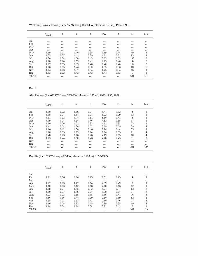
Waskesiu, Saskatchewan (Lat 53°55′N Long 106°04′W, elevation 550 m), 1994-1999.

τa500 σ α σ PW σ N Mo.

Jan … … … … … … … …Feb … … … … … … … …Mar … … … … … … … …Apr … … … … … … … …May 0.19 0.11 1.40 0.35 1.19 0.48 49 4Jun 0.23 0.27 1.41 0.39 1.61 0.51 93 4Jul 0.20 0.24 1.50 0.43 2.03 0.53 133 5Aug 0.18 0.20 1.55 0.41 1.95 0.48 144 6Sep 0.07 0.05 1.35 0.48 1.40 0.40 112 5Oct 0.06 0.05 1.24 0.50 0.95 0.36 68 5Nov 0.04 0.03 1.37 0.54 0.75 0.34 16 1Dec 0.03 0.02 1.43 0.43 0.44 0.13 6 1YEAR … … … … … … 621 31

Brazil

Alta Floresta (Lat 09°55′S Long 56°00′W, elevation 175 m), 1993-1995, 1999.

τa500 σ α σ PW σ N Mo.

Jan 0.09 0.03 0.66 0.24 5.41 0.12 4 1Feb 0.08 0.04 0.57 0.27 5.22 0.29 13 1Mar 0.11 0.12 0.74 0.51 5.10 0.41 8 1Apr 0.09 0.04 0.98 0.46 4.82 0.55 17 1May 0.10 0.06 1.21 0.53 4.61 0.52 23 1Jun 0.11 0.04 1.30 0.62 3.69 0.69 29 2Jul 0.16 0.12 1.50 0.46 2.94 0.44 55 2Aug 1.18 0.65 1.89 0.24 2.84 0.55 81 4Sep 1.48 0.73 1.66 0.28 4.19 0.65 80 4Oct 0.63 0.24 1.50 0.26 4.76 0.43 31 2Nov … … … … … … … …Dec … … … … … … … …YEAR … … … … … … 341 19

Brasilia (Lat 15°55′S Long 47°54′W, elevation 1100 m), 1993-1995.

τa500 σ α σ PW σ N Mo.

Jan … … … … … … … …Feb 0.11 0.06 1.04 0.23 2.51 0.25 4 1Mar … … … … … … … …Apr 0.07 0.03 0.77 0.14 2.99 0.29 7 1May 0.10 0.03 1.12 0.18 2.60 0.16 12 1Jun 0.08 0.04 0.95 0.32 1.74 0.51 63 3Jul 0.09 0.07 0.96 0.27 1.70 0.27 71 3Aug 0.23 0.23 1.15 0.35 1.56 0.41 76 3Sep 0.56 0.36 1.44 0.29 2.10 0.69 52 2Oct 0.35 0.21 1.32 0.42 2.60 0.46 27 2Nov 0.16 0.08 0.83 0.45 2.89 0.55 19 2Dec 0.14 0.04 0.64 0.34 3.21 0.41 6 1YEAR … … … … … … 337 19

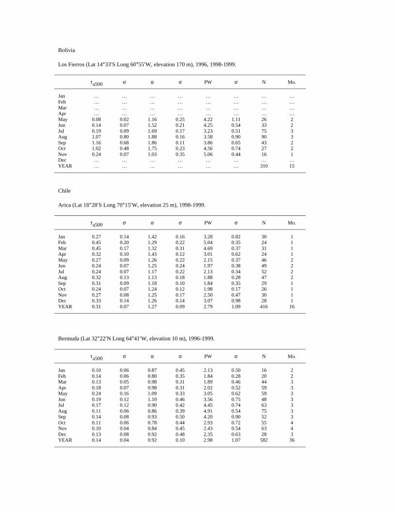
Bolivia

Los Fierros (Lat 14°33′S Long 60°55′W, elevation 170 m), 1996, 1998-1999.

τa500 σ α σ PW σ N Mo.

Jan … … … … … … … …Feb … … … … … … … …Mar … … … … … … … …Apr … … … … … … … …May 0.08 0.02 1.16 0.25 4.22 1.11 26 2Jun 0.14 0.07 1.52 0.21 4.25 0.54 33 2Jul 0.19 0.09 1.69 0.17 3.23 0.51 75 3Aug 1.07 0.80 1.88 0.16 3.58 0.90 90 3Sep 1.16 0.68 1.86 0.11 3.86 0.65 43 2Oct 1.02 0.48 1.75 0.23 4.56 0.74 27 2Nov 0.24 0.07 1.03 0.35 5.06 0.44 16 1Dec … … … … … … … …YEAR … … … … … … 310 15

Chile

Arica (Lat 18°28′S Long 70°15′W, elevation 25 m), 1998-1999.

τa500 σ α σ PW σ N Mo.

Jan 0.27 0.14 1.42 0.16 3.28 0.82 30 1Feb 0.45 0.20 1.29 0.22 5.04 0.35 24 1Mar 0.45 0.17 1.32 0.31 4.69 0.37 31 1Apr 0.32 0.10 1.43 0.12 3.01 0.62 24 1May 0.27 0.09 1.26 0.22 2.15 0.37 46 2Jun 0.24 0.07 1.25 0.24 1.97 0.38 49 2Jul 0.24 0.07 1.17 0.22 2.13 0.34 52 2Aug 0.32 0.13 1.13 0.18 1.88 0.28 47 2Sep 0.31 0.09 1.18 0.10 1.84 0.35 29 1Oct 0.24 0.07 1.24 0.12 1.98 0.17 26 1Nov 0.27 0.08 1.25 0.17 2.50 0.47 30 1Dec 0.33 0.14 1.26 0.14 3.07 0.98 28 1YEAR 0.31 0.07 1.27 0.09 2.79 1.09 416 16

Bermuda (Lat 32°22′N Long 64°41′W, elevation 10 m), 1996-1999.

τa500 σ α σ PW σ N Mo.

Jan 0.10 0.06 0.87 0.45 2.13 0.50 16 2Feb 0.14 0.06 0.80 0.35 1.84 0.28 20 2Mar 0.13 0.05 0.98 0.31 1.89 0.46 44 3Apr 0.18 0.07 0.98 0.31 2.02 0.52 59 3May 0.24 0.16 1.09 0.33 3.05 0.62 59 3Jun 0.19 0.12 1.10 0.46 3.56 0.75 48 3Jul 0.17 0.12 0.90 0.42 4.45 0.74 63 3Aug 0.11 0.06 0.86 0.39 4.91 0.54 75 3Sep 0.14 0.08 0.93 0.50 4.20 0.90 52 3Oct 0.11 0.06 0.78 0.44 2.93 0.72 55 4Nov 0.10 0.04 0.84 0.45 2.43 0.54 63 4Dec 0.13 0.08 0.92 0.48 2.35 0.63 28 3YEAR 0.14 0.04 0.92 0.10 2.98 1.07 582 36

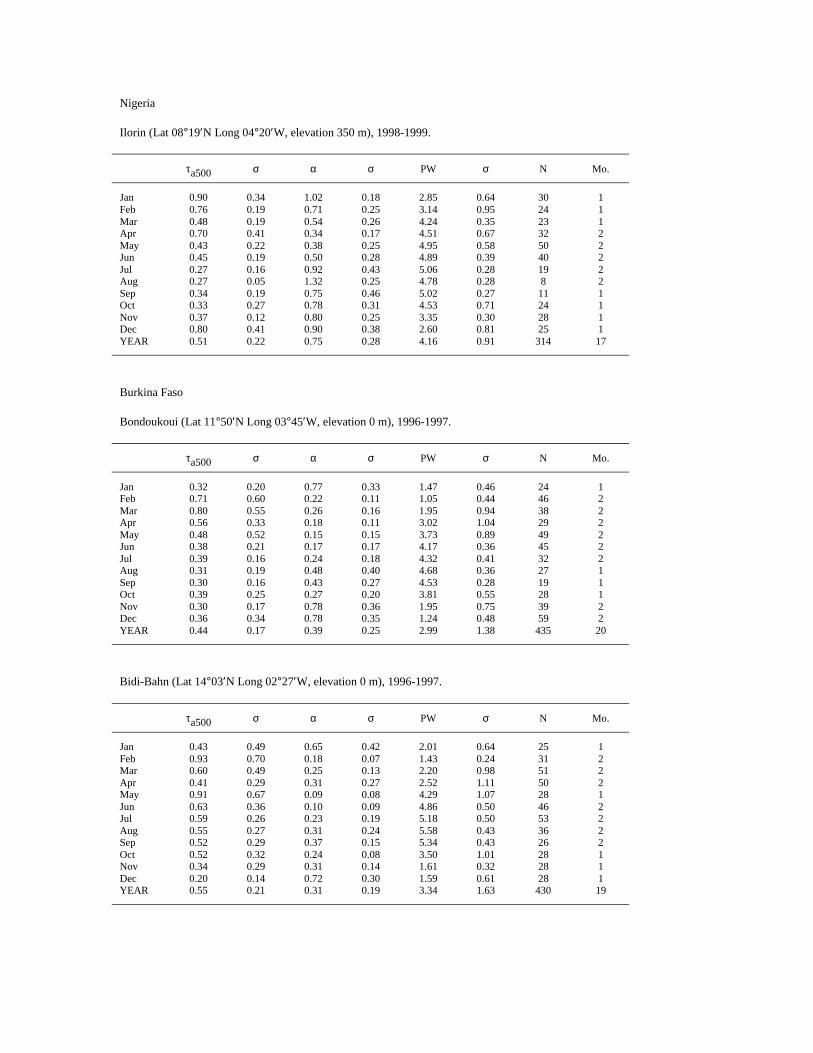
Nigeria

Ilorin (Lat 08°19′N Long 04°20′W, elevation 350 m), 1998-1999.

τa500 σ α σ PW σ N Mo.

Jan 0.90 0.34 1.02 0.18 2.85 0.64 30 1Feb 0.76 0.19 0.71 0.25 3.14 0.95 24 1Mar 0.48 0.19 0.54 0.26 4.24 0.35 23 1Apr 0.70 0.41 0.34 0.17 4.51 0.67 32 2May 0.43 0.22 0.38 0.25 4.95 0.58 50 2Jun 0.45 0.19 0.50 0.28 4.89 0.39 40 2Jul 0.27 0.16 0.92 0.43 5.06 0.28 19 2Aug 0.27 0.05 1.32 0.25 4.78 0.28 8 2Sep 0.34 0.19 0.75 0.46 5.02 0.27 11 1Oct 0.33 0.27 0.78 0.31 4.53 0.71 24 1Nov 0.37 0.12 0.80 0.25 3.35 0.30 28 1Dec 0.80 0.41 0.90 0.38 2.60 0.81 25 1YEAR 0.51 0.22 0.75 0.28 4.16 0.91 314 17

Burkina Faso

Bondoukoui (Lat 11°50′N Long 03°45′W, elevation 0 m), 1996-1997.

τa500 σ α σ PW σ N Mo.

Jan 0.32 0.20 0.77 0.33 1.47 0.46 24 1Feb 0.71 0.60 0.22 0.11 1.05 0.44 46 2Mar 0.80 0.55 0.26 0.16 1.95 0.94 38 2Apr 0.56 0.33 0.18 0.11 3.02 1.04 29 2May 0.48 0.52 0.15 0.15 3.73 0.89 49 2Jun 0.38 0.21 0.17 0.17 4.17 0.36 45 2Jul 0.39 0.16 0.24 0.18 4.32 0.41 32 2Aug 0.31 0.19 0.48 0.40 4.68 0.36 27 1Sep 0.30 0.16 0.43 0.27 4.53 0.28 19 1Oct 0.39 0.25 0.27 0.20 3.81 0.55 28 1Nov 0.30 0.17 0.78 0.36 1.95 0.75 39 2Dec 0.36 0.34 0.78 0.35 1.24 0.48 59 2YEAR 0.44 0.17 0.39 0.25 2.99 1.38 435 20

Bidi-Bahn (Lat 14°03′N Long 02°27′W, elevation 0 m), 1996-1997.

τa500 σ α σ PW σ N Mo.

Jan 0.43 0.49 0.65 0.42 2.01 0.64 25 1Feb 0.93 0.70 0.18 0.07 1.43 0.24 31 2Mar 0.60 0.49 0.25 0.13 2.20 0.98 51 2Apr 0.41 0.29 0.31 0.27 2.52 1.11 50 2May 0.91 0.67 0.09 0.08 4.29 1.07 28 1Jun 0.63 0.36 0.10 0.09 4.86 0.50 46 2Jul 0.59 0.26 0.23 0.19 5.18 0.50 53 2Aug 0.55 0.27 0.31 0.24 5.58 0.43 36 2Sep 0.52 0.29 0.37 0.15 5.34 0.43 26 2Oct 0.52 0.32 0.24 0.08 3.50 1.01 28 1Nov 0.34 0.29 0.31 0.14 1.61 0.32 28 1Dec 0.20 0.14 0.72 0.30 1.59 0.61 28 1YEAR 0.55 0.21 0.31 0.19 3.34 1.63 430 19

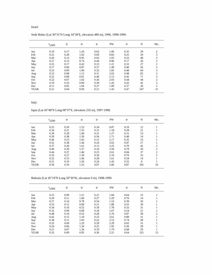
Israel

Sede Boker (Lat 30°31′N Long 34°28′E, elevation 480 m), 1996, 1998-1999.

τa500 σ α σ PW σ N Mo.

Jan 0.19 0.17 1.20 0.62 1.06 0.35 29 2Feb 0.21 0.28 1.02 0.69 0.83 0.25 29 3Mar 0.20 0.13 0.95 0.63 1.03 0.23 48 3Apr 0.27 0.13 0.74 0.44 0.96 0.17 26 2May 0.25 0.17 0.42 0.23 1.21 0.33 27 2Jun 0.17 0.06 0.87 0.37 1.49 0.40 56 3Jul 0.23 0.09 1.06 0.32 1.85 0.48 64 3Aug 0.23 0.08 1.12 0.31 2.02 0.48 85 3Sep 0.22 0.08 0.91 0.40 2.13 0.45 71 3Oct 0.22 0.07 1.02 0.36 2.03 0.44 44 2Nov 0.19 0.10 0.90 0.39 1.45 0.43 42 3Dec 0.11 0.05 1.04 0.37 1.09 0.37 26 2YEAR 0.21 0.04 0.94 0.21 1.43 0.47 547 31

Italy

Ispra (Lat 45°48′N Long 08°37′E, elevation 235 m), 1997-1998.

τa500 σ α σ PW σ N Mo.

Jan 0.25 0.20 1.53 0.34 0.87 0.19 12 1Feb 0.34 0.21 1.55 0.15 1.18 0.28 21 1Mar 0.39 0.28 1.49 0.31 1.27 0.31 23 1Apr 0.39 0.38 1.50 0.36 1.71 0.48 14 1May 0.46 0.23 1.62 0.15 2.17 0.35 23 1Jun 0.52 0.38 1.44 0.24 3.02 0.87 27 1Jul 0.37 0.30 1.61 0.13 3.25 0.70 42 2Aug 0.40 0.20 1.57 0.16 3.50 0.78 50 2Sep 0.44 0.37 1.46 0.23 2.61 0.84 37 2Oct 0.35 0.27 1.39 0.30 2.10 0.70 32 2Nov 0.22 0.15 1.46 0.28 1.61 0.54 14 1Dec 0.21 0.10 1.56 0.24 1.43 0.25 6 1YEAR 0.36 0.10 1.52 0.07 2.06 0.87 301 16

Bahrain (Lat 26°19′N Long 50°30′W, elevation 0 m), 1998-1999.

τa500 σ α σ PW σ N Mo.

Jan 0.23 0.09 1.21 0.21 1.84 0.64 22 1Feb 0.29 0.11 1.00 0.27 2.29 0.70 14 1Mar 0.27 0.14 0.78 0.54 1.53 0.39 26 1Apr 0.33 0.12 0.68 0.21 1.88 0.55 30 1May 0.34 0.16 0.52 0.18 1.78 0.53 31 1Jun 0.32 0.09 0.68 0.18 1.67 0.24 21 1Jul 0.48 0.19 0.55 0.28 2.76 0.87 30 2Aug 0.45 0.15 1.10 0.23 3.61 0.89 31 1Sep 0.38 0.11 1.03 0.22 3.12 0.74 28 1Oct 0.25 0.09 1.25 0.29 2.29 0.65 31 1Nov 0.24 0.06 1.34 0.25 1.95 0.30 28 1Dec 0.21 0.07 1.26 0.19 1.79 0.68 29 1YEAR 0.32 0.09 0.95 0.30 2.21 0.64 321 13

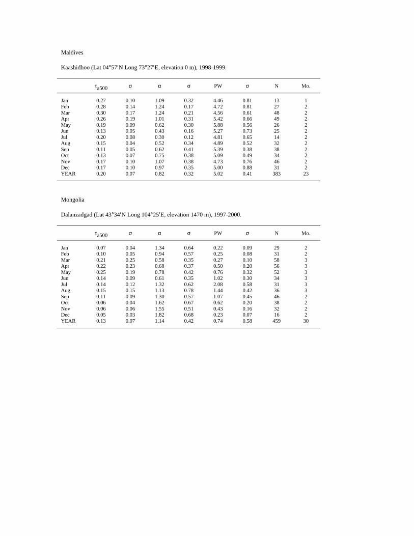
Maldives

Kaashidhoo (Lat 04°57′N Long 73°27′E, elevation 0 m), 1998-1999.

τa500 σ α σ PW σ N Mo.

Jan 0.27 0.10 1.09 0.32 4.46 0.81 13 1Feb 0.28 0.14 1.24 0.17 4.72 0.81 27 2Mar 0.30 0.17 1.24 0.21 4.56 0.61 48 2Apr 0.26 0.19 1.01 0.31 5.42 0.66 49 2May 0.19 0.09 0.62 0.30 5.88 0.56 26 2Jun 0.13 0.05 0.43 0.16 5.27 0.73 25 2Jul 0.20 0.08 0.30 0.12 4.81 0.65 14 2Aug 0.15 0.04 0.52 0.34 4.89 0.52 32 2Sep 0.11 0.05 0.62 0.41 5.39 0.38 38 2Oct 0.13 0.07 0.75 0.38 5.09 0.49 34 2Nov 0.17 0.10 1.07 0.38 4.73 0.76 46 2Dec 0.17 0.10 0.97 0.35 5.00 0.88 31 2YEAR 0.20 0.07 0.82 0.32 5.02 0.41 383 23

Mongolia

Dalanzadgad (Lat 43°34′N Long 104°25′E, elevation 1470 m), 1997-2000.

τa500 σ α σ PW σ N Mo.

Jan 0.07 0.04 1.34 0.64 0.22 0.09 29 2Feb 0.10 0.05 0.94 0.57 0.25 0.08 31 2Mar 0.21 0.25 0.58 0.35 0.27 0.10 58 3Apr 0.22 0.23 0.68 0.37 0.50 0.20 56 3May 0.25 0.19 0.78 0.42 0.76 0.32 52 3Jun 0.14 0.09 0.61 0.35 1.02 0.30 34 3Jul 0.14 0.12 1.32 0.62 2.08 0.58 31 3Aug 0.15 0.15 1.13 0.78 1.44 0.42 36 3Sep 0.11 0.09 1.30 0.57 1.07 0.45 46 2Oct 0.06 0.04 1.62 0.67 0.62 0.20 38 2Nov 0.06 0.06 1.55 0.51 0.43 0.16 32 2Dec 0.05 0.03 1.82 0.68 0.23 0.07 16 2YEAR 0.13 0.07 1.14 0.42 0.74 0.58 459 30