An Elastic-Viscous-Plastic Sea Ice Model

formulated on Arakawa B and C Grids

Sylvain Bouillona, c, 1 ,Miguel Angel Morales Maquedab

Vincent Legatc and Thierry Fichefeta

a G. Lemaıtre Institute of Astronomy and Geophysics (ASTR),Universite catholique de Louvain, 2 Chemin du Cyclotron, B-1348

Louvain-la-Neuve, Belgium.b Proudman Oceanographic Laboratory (POL),

6 Brownlow Street, Liverpool L3 5DA, United Kingdom.c Center for Systems Engineering and Applied Mechanics (CESAME),

Universite catholique de Louvain, 4 Avenue G. Lemaıtre, B-1348Louvain-la-Neuve, Belgium.

Key words: Sea ice, Coupled sea ice-ocean model, Elastic-viscous-plastic rheology,Model grid

1 Introduction

The dynamic component of most sea ice models designed for climate studiesis based on the ice momentum balance formulation of Hibler (1979). In thismodel, sea ice is assumed to be a non-linear viscous-plastic (VP) materialwhose resistance to deformation depends on its instantaneous state of motionand several large-scale scalar properties, such as ice thickness and lead frac-tional area. The VP formulation of Hibler (1979) has known many successes,but it is computationally expensive and not well suited for efficient parallelintegrations. The numerical method first used to solve the VP dynamics was arelatively slow implicit point relaxation method (Hibler, 1979). More efficientimplicit methods have been proposed subsequently, namely, the line relax-ation method (Zhang and Hibler, 1997) and the alternating direction implicitmethod (Zhang and Rothrock, 2000). However, the most popular alternativefor the calculation of the VP dynamics is the elastic-viscous-plastic (EVP) for-mulation of Hunke and Dukowicz (1997). Distinctive advantages of the EVP

1 Corresponding author. E-mail: sylvain.bouillon@uclouvain.be, Tel: +32 10 47 3067, Fax: +32 10 47 47 22

Preprint

dynamics over the VP dynamics is that it is much simpler to program andcan be solved explicitly in time, thus easing parallelization.

Because of the appealing numerical properties of the EVP dynamics, a growingnumber of large-scale, coupled ocean-sea ice and atmosphere-ocean-sea icemodels have adopted this formulation (e.g., Randall et al., 2007). Promptedby this trend, we have incorporated the EVP rheology in the Louvain-la-Neuvesea-Ice Model, LIM (Fichefet and Morales Maqueda, 1997, 1999). LIM is thedefault sea ice module of the Nucleus for European Modelling of the Ocean(NEMO, http://www.locean-ipsl.upmc.fr/NEMO/). LIM is also widely usedoutside the NEMO project. It is the sea ice component of the global coupledsea ice-ocean model CLIO (Goosse and Fichefet, 1999), and has been coupledto the ocean general circulation models OPA (Ocean PArallelise), which is theprecursor of NEMO (Madec et al., 1999), and MOM3 (Modular Ocean Model,version 3, Hofmann and Morales Maqueda (2006)), as well as to Earth systemmodels of intermediate complexity CLIMBER3α (Montoya et al., 2005) andLOVECLIM (Driesschaert et al., 2007), and to the climate general circulationmodel IPSL-CM4 (Marti et al., 2008). Simulations with the coupled OPA-LIM model have been analyzed by Timmermann et al. (2005), and a newversion of the model including an arbitrary number of ice thickness categoriesand a multi-layer halo-thermodynamic module has been recently completedby Vancoppenolle et al. (2008).

Official releases of LIM have, until now, employed the VP dynamics formula-tion, although a cavitating fluid approach was also briefly tested by Fichefetand Morales Maqueda (1997), and the versions of LIM coupled to MOM3 andCLIMBER3α do incorporate already implementations of the EVP dynamics.However, this work is the first attempt to evaluate the impact of the EVPparameterization on LIM.

We have tested three versions of the EVP dynamics in LIM, namely, the mostrecent bilinear discretization of Hunke and Dukowicz (2002) on an ArakawaB grid, and two simpler discretizations that we will describe here in full, thefirst of which is also formulated on a B grid, while the second is for a Cgrid. We present results of simulations with the coupled OPA-LIM model,each employing one of the three EVP formulations that we have just referredto. For comparison, a fourth integration was also carried out with the originalVP parameterization. Reassuringly, all three EVP discretizations produce verysimilar results. However, the C grid version is the one that has been chosenfor use within the NEMO project, as it is faster than any of the other two andaffords a more direct coupling with the ocean component of NEMO, which isan updated version of OPA and is also discretized on a C grid.

The article is organized as follows. Section 2 succinctly describes LIM. Section3 discusses issues pertaining to the new discretization of the model dynamics,

2

specially as regards the new implementation on a C grid. Section 4 presentsan intercomparison of key results from the numerical simulations. Conclusionsare presented in Section 5.

2 Model description

The version of LIM used in this study (LIM2) is described in full detail in Tim-mermann et al. (2005) and references therein. Therefore, only a brief summaryof the model, with emphasis on its dynamics, is given here.

The thermodynamic part of LIM (Fichefet and Morales Maqueda, 1997, 1999)uses a three-layer model for the vertical heat conduction within snow and ice.The storage of latent heat in brine pockets is taken into account, and seaice growth and decay rates are obtained from the ice energy budget. Air-ice and air-ocean heat fluxes are computed using empirical parameterizationsdescribed by Goosse (1997), and the ice-ocean heat flux is computed as inMcPhee (1992).

The model dynamics are based on the two-category (consolidated ice plusleads) approach of Hibler (1979). This two-category ice cover is treated as atwo-dimensional compressible fluid driven by winds and oceanic currents. Seaice resist deformation with a strength which increases monotonically with icethickness and concentration.

The conservation of linear momentum for sea ice is expressed as in Lepparanta(2005) by

mut = ∇ · σ + A (τ a + τw) − mfk × u − mg∇η, (1)

where m is the ice mass per unit area, u is the ice velocity, σ is the internalstress tensor, A is the ice area fraction, or concentration, τ a is the wind stress,τw is the ocean stress (typically quadratic), f is the Coriolis parameter, k is anupward pointing unit vector, g is the gravity acceleration and η is the oceansurface elevation with respect to zero sea level. Note that the momentumadvection is being ignored in (1) and that the wind and ocean stresses aremultiplied by the ice concentration as suggested by Connolley et al. (2004).

Calculation of sea ice internal forces in LIM has customarily been done usingthe VP approach of Hibler (1979), which, in practice, is a particular case of theEVP formulation of Hunke and Dukowicz (1997). A description of the generalframework for the VP and EVP formulations of the ice internal stresses isgiven in Hunke and Dukowicz (2002) and Hunke and Lipscomb (2006). Forcompletion, we reproduce here the key elements of such a framework. Let us

3

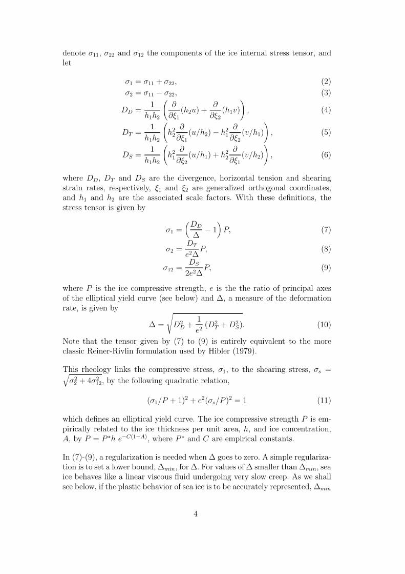
denote σ11, σ22 and σ12 the components of the ice internal stress tensor, andlet

σ1 = σ11 + σ22, (2)

σ2 = σ11 − σ22, (3)

DD =1

h1h2

(

∂

∂ξ1(h2u) +

∂

∂ξ2(h1v)

)

, (4)

DT =1

h1h2

(

h22

∂

∂ξ1(u/h2) − h2

1

∂

∂ξ2(v/h1)

)

, (5)

DS =1

h1h2

(

h21

∂

∂ξ2(u/h1) + h2

2

∂

∂ξ1(v/h2)

)

, (6)

where DD, DT and DS are the divergence, horizontal tension and shearingstrain rates, respectively, ξ1 and ξ2 are generalized orthogonal coordinates,and h1 and h2 are the associated scale factors. With these definitions, thestress tensor is given by

σ1 =(

DD

∆− 1

)

P, (7)

σ2 =DT

e2∆P, (8)

σ12 =DS

2e2∆P, (9)

where P is the ice compressive strength, e is the the ratio of principal axesof the elliptical yield curve (see below) and ∆, a measure of the deformationrate, is given by

∆ =

√

D2D +

1

e2(D2

T + D2S). (10)

Note that the tensor given by (7) to (9) is entirely equivalent to the moreclassic Reiner-Rivlin formulation used by Hibler (1979).

This rheology links the compressive stress, σ1, to the shearing stress, σs =√

σ22 + 4σ2

12, by the following quadratic relation,

(σ1/P + 1)2 + e2(σs/P )2 = 1 (11)

which defines an elliptical yield curve. The ice compressive strength P is em-pirically related to the ice thickness per unit area, h, and ice concentration,A, by P = P ∗h e−C(1−A), where P ∗ and C are empirical constants.

In (7)-(9), a regularization is needed when ∆ goes to zero. A simple regulariza-tion is to set a lower bound, ∆min, for ∆. For values of ∆ smaller than ∆min, seaice behaves like a linear viscous fluid undergoing very slow creep. As we shallsee below, if the plastic behavior of sea ice is to be accurately represented, ∆min

4

must be sufficiently small (say 10−9 s−1 or less). Note that ∆min is directlyrelated to the ζmax parameter used in Hibler (1979) by ζmax = P/ (2∆min).

An alternative regularization was proposed by Hunke and Dukowicz (1997),and it consists in introducing time dependence and an artificial elastic termin (7)-(9), leading to the EVP formulation:

2Tσ1,t + σ1 =(

DD

∆− 1

)

P, (12)

2T

e2σ2,t + σ2 =

DT

e2∆P, (13)

2T

e2σ12,t + σ12 =

DS

2e2∆P, (14)

where T is a time scale that controls the rate of damping of elastic waves. Notethat, while (12)-(14) become (7)-(9) in the steady state, static flow in the EVPrheology is represented by an elastic deformation, and so imposing a minimumvalue of ∆ is no longer necessary. Hunke and Dukowicz (1997) showed that thenumerical solution of (1) in combination with (12)-(14) does indeed convergeto the VP stationary solution as long as the elastic time scale T is severaltimes smaller than the time scale of variation of the external forcing.

The components of the internal stress force are (Hunke and Dukowicz, 2002):

2F1 =1

h1

∂σ1

∂ξ1+

1

h1h22

∂(h22σ2)

∂ξ1+

2

h21h2

∂(h21σ12)

∂ξ2, (15)

2F2 =1

h2

∂σ1

∂ξ2−

1

h21h2

∂(h21σ2)

∂ξ2+

2

h1h22

∂(h22σ12)

∂ξ1. (16)

3 Discretizations of the model dynamics

Numerical stability analyses show that explicit time integration of the VP dy-namics would be very expensive. Indeed, the critical time step for a stable ex-plicit VP scheme is about 1 s for a 100-km grid, and scales as d2, where d is thehorizontal resolution (Hunke and Dukowicz, 1997). Given such a prohibitivelysmall explicit time step, an implicit method of integration is required. In LIM,the implicit VP solver currently used closely follows the successive relaxationmethod of Hibler (1979) with under-relaxation. For typical spatial resolutionsof 50 km to 100 km, daily wind forcing variability and time step, ∆t, of half aday to a quarter of a day, a few hundred iterations per time step are requiredfor the relaxation scheme to converge. A type of predictor-corrector schemeis used for the ice dynamics, whereby, starting from a solution at time t, anintermediate solution is first evaluated at time t + ∆t/2. The solution at timet + ∆t is then calculated with the non-linear terms in the internal stress and

5

ice-ocean stress terms centred at t+∆t/2. For time steps of between 1 day anda few hours, the solution thus obtained may be a rather crude approximationof the real plastic flow, and the resulting stress state is likely to lie away fromthe yield curve. Accuracy can be improved by repeating the predictor-correctorcalculation several times, say n, with a subcycling time step ∆t/n.

In contrast to the VP dynamics, the EVP dynamics can be solved explicitlywith time steps that can be few orders of magnitude larger than the maximumpermissible explicit time step for the VP formulation. In addition, this max-imum time step scales linearly, rather than quadratically, with d, although italso depends on the time scale T (Hunke and Dukowicz, 1997; Hunke and Lip-scomb, 2006). The explicit numerical solution of the EVP equations is thussignificantly less expensive than implicit methods for the VP formulation.Moreover, the convergence of the calculated stress state toward the ellipticyield curve is relatively fast because all the non linear terms in (1) are reeval-uated every time step. The EVP scheme is also easy to parallelize, and givesa higher speedup factor (measured as the ratio between wall clock serial timeand wall clock parallel time) than parallel implementations of the VP method(Hunke and Zhang, 1999).

3.1 B grid discretization

We have introduced three discretizations of the EVP dynamics in LIM. Thefirst discretization is the one formulated by Hunke and Dukowicz (2002).These authors use a sophisticated variational method to calculate the in-ternal stress force in discrete generalized orthogonal curvilinear coordinates.Formally working on a B grid, and using bilinear approximations for the icevelocities over a given grid cell, the components of the strain rate and internalstress tensors are computed at the corners of each grid cell, thus requiringfour computations per tensor component per grid cell. As Hunke and Dukow-icz (2002) emphasize, this approach greatly helps to mitigate checkerboardmode solutions that are frequently generated on the B grid.

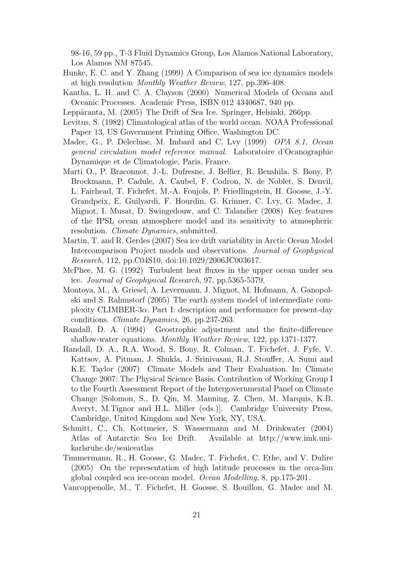
The discretization of Hunke and Dukowicz (2002) is computationally expen-sive because it requires four calculations of each component of the strain rateand internal stress tensors per grid cell. As an alternative, we have also imple-mented in LIM a naıve, centred difference discretization on the B grid. Thissecond discretization is constructed as follows. On the B grid, consider a gridcell whose central, or scalar, point has indexes i, j. As shown in Fig. 1, the in-dexes of the four corners, or velocity points, of the cell are then i−1/2, j−1/2(left, bottom corner), i + 1/2, j − 1/2 (right, bottom corner), i + 1/2, j + 1/2(right, top corner), and i − 1/2, j + 1/2 (left, top corner). Analogously, theindexes of the four mid points on the grid cell sides, or transport points, are

6

i−1/2, j (left, centre point), i, j−1/2 (centre, bottom point), i+1/2, j (right,centre point), and i, j + 1/2 (centre, top point). Denoting the grid elementse1 = h1∆ξ1 and e2 = h2∆ξ2, where ∆ξ1 and ∆ξ2 are the spatial steps in thetwo orthogonal directions, the components of the strain rate tensor are givenby

2 e1i,j e2i,j DDi,j =

e2i+1/2,j

(

ui+1/2,j+1/2 + ui+1/2,j−1/2

)

− e2i−1/2,j

(

ui−1/2,j+1/2 + ui−1/2,j−1/2

)

+

e1i,j+1/2

(

vi+1/2,j+1/2 + vi−1/2,j+1/2

)

−e1i,j−1/2

(

vi+1/2,j−1/2 + vi−1/2,j−1/2

)

,

(17)

2 e1i,j e2i,j DT i,j =

e22i,j

(

ui+1/2,j+1/2 + ui+1/2,j−1/2

e2i+1/2,j

−ui−1/2,j+1/2 + ui−1/2,j−1/2

e2i−1/2,j

)

−

e12i,j

(

vi+1/2,j+1/2 + vi−1/2,j+1/2

e1i,j+1/2

−vi+1/2,j−1/2 + vi−1/2,j−1/2

e1i,j−1/2

)

, (18)

2 e1i,j e2i,j DSi,j =

e12i,j

(

ui+1/2,j+1/2 + ui−1/2,j+1/2

e1i,j+1/2

−ui+1/2,j−1/2 + ui−1/2,j−1/2

e1i,j−1/2

)

+

e22i,j

(

vi+1/2,j+1/2 + vi+1/2,j−1/2

e2i+1/2,j

−vi−1/2,j+1/2 + vi−1/2,j−1/2

e2i−1/2,j

)

. (19)

All three quantities DDi,j, DT i,j and DSi,j are defined on the centre of the gridcells. The components of the internal stress tensor, also defined on the gridcell centres, can now be evaluated by solving (12), (13) and (14). The internalstress force components, F1 and F2, which are defined on the grid cell corners,can then be calculated as

4 e1i+1/2,j+1/2 e2i+1/2,j+1/2 F1i+1/2,j+1/2 =

e2i+1/2,j+1/2

(

σ1i+1,j+1 + σ1i+1,j − σ1i,j+1 − σ1i,j

)

+

1

e2i+1/2,j+1/2

(

e22i+1,j+1/2

(

σ2i+1,j+1 + σ2i+1,j

)

− e22i,j+1/2

(

σ2i,j+1 + σ2i,j

))

+

2

e1i+1/2,j+1/2

(

e12i+1/2,j+1

(

σ12i+1,j+1 + σ12i,j+1

)

− e12i+1/2,j

(

σ12i+1,j + σ12i,j

))

.

(20)

7

4 e1i+1/2,j+1/2 e2i+1/2,j+1/2 F2i+1/2,j+1/2 =

e1i+1/2,j+1/2

(

σ1i+1,j+1 + σ1i,j+1 − σ1i+1,j − σ1i,j

)

−

1

e1i+1/2,j+1/2

(

e12i+1/2,j+1

(

σ2i+1,j+1 + σ2i,j+1

)

− e12i+1/2,j

(

σ2i+1,j + σ2i,j

))

+

2

e2i+1/2,j+1/2

(

e22i+1,j+1/2

(

σ12i+1,j+1 + σ12i+1,j

)

− e22i,j+1/2

(

σ12i,j+1 + σ12i,j

))

.

(21)

The discretization in time of both the bilinear and centred difference formu-lations on the B grid follows that of Hunke and Lipscomb (2006), and is

2Tσ1

k+1 − σ1k

∆t+ σ1

k+1 =

(

DkD

∆k− 1

)

P, (22)

2T

e2

σ2k+1 − σ2

k

∆t+ σk+1

2 =Dk

T

e2∆kP, (23)

2T

e2

σ12k+1 − σ12

k

∆t+ σk+1

12 =Dk

S

2e2∆kP, (24)

muk+1 − uk

∆t=

F1k+1 + A

(

τa1 + cDρo|uo − uk|(

uo − uk+1))

+ mfvk+1 − mg1

h1

∂η

∂ξ1, (25)

mvk+1 − vk

∆t=

F2k+1 + A

(

τa2 + cDρo|uo − uk|(

vo − vk+1))

− mfuk+1 − mg1

h2

∂η

∂ξ2, (26)

where, for expediency, we have dropped spatial sub-indexes, the super-indexesk and k + 1 denote variables evaluated at times k∆t and (k + 1)∆t, respec-tively, where ∆t is the dynamics time step, cD is the ice-ocean drag coefficient,ρo is the reference density of seawater and uo ≡ (uo, vo) is the surface oceaniccurrent. The ice compressive strength P is updated only every thermodynam-ics and ice transport time step, which is normally orders of magnitude largerthan ∆t.

3.2 C grid discretization

For each sea ice-ocean coupling step, the B grid discretization requires inter-polation of sea ice fields onto the ocean grid, which is of Arakawa C type,and, likewise, surface oceanic fields need also to be interpolated onto the sea

8

ice grid. Within the sea ice model, interpolation of sea ice drift rates onto themidpoint of grid cell sides is also required before transport of sea ice scalarsis calculated. Such interpolations would be avoided if a C grid were used inthe calculation of the sea ice dynamics, which is why we have also formulateda centred difference version of the EVP dynamics (see Kantha and Clayson(2000) for a C grid, centred difference formulation of the VP case). Anotherimportant reason why a C grid is desirable is that, with no slip boundaryconditions, transport of scalar properties through narrow straits and passageswith a width of just one single grid cell is possible on a C grid, while it isprecluded on a B grid.

Using the same indexing conventions as for the B grid, the discretization ofthe strain rate tensor is

e1i,j e2i,j DDi,j =

e2i+1/2,j ui+1/2,j − e2i−1/2,j ui−1/2,j + e1i,j+1/2 vi,j+1/2 − e1i,j−1/2 vi,j−1/2, (27)

e1i,j e2i,j DT i,j = e22i,j

(

ui+1/2,j

e2i+1/2,j

−ui−1/2,j

e2i−1/2,j

)

−e12i,j

(

vi,j+1/2

e1i,j+1/2

−vi,j−1/2

e1i,j−1/2

)

,

(28)

e1i+1/2,j+1/2 e2i+1/2,j+1/2 DSi+1/2,j+1/2 =

e12i+1/2,j+1/2

(

ui+1/2,j+1

e1i+1/2,j+1

−ui+1/2,j

e1i+1/2,j

)

+e22i+1/2,j+1/2

(

vi+1,j+1/2

e2i+1,j+1/2

−vi,j+1/2

e2i,j+1/2

)

.

(29)

Note that the components DD, DT , σ1 and σ2 are all defined on the cell cen-tres, while DS and σ12 are defined on the corners. The internal stress forcecomponent F1 is located on u points and F2 on v points. In a C grid, thevelocity components are ideally located for the calculation of the componentsof the strain rate and the internal stress tensors, requiring fewer interpola-tions than on the B grid. As the invariant ∆ is used to compute the internalstress components, it needs, however, to be computed both on cell centres andcorners, and so, for the purpose of the calculation of ∆, DD and DT must beinterpolated onto cell corners, while DS must be interpolated onto cell centres.The expression for DD on cell corners is

(e1i,j+1/2 + e1i+1,j+1/2)(e2i+1/2,j + e2i+1/2,j+1)DDi+1/2,j+1/2 =

e2i+1/2,j+1

(

e1i+1,j+1/2 DDi,j + e1i,j+1/2 DDi+1,j

)

+

e2i+1/2,j

(

e1i+1,j+1/2 DDi,j+1 + e1i,j+1/2 DDi+1,j+1

)

, (30)

with an analogous formula for DT i+1/2,j+1/2, while the centred value of DS is

9

given by

4 DSi,j = DSi−1/2,j−1/2 + DSi+1/2,j−1/2 + DSi+1/2,j+1/2 + DSi−1/2,j+1/2. (31)

The internal stress force components on the C grid are

2 e1i+1/2,j e2i+1/2,j F1i+1/2,j =

e2i+1/2,j

(

σ1i+1,j − σ1i,j

)

+1

e2i+1/2,j

(

e22i+1,jσ2i+1,j − e2

2i,jσ2i,j

)

+

2

e1i+1/2,j

(

e12i+1/2,j+1/2σ12i+1/2,j+1/2 − e1

2i+1/2,j−1/2σ12i+1/2,j−1/2

)

, (32)

2 e1i,j+1/2 e2i,j+1/2 F2i,j+1/2 =

e1i,j+1/2

(

σ1i,j+1 − σ1i,j

)

−1

e1i,j+1/2

(

e12i,j+1σ2i,j+1 − e1

2i,jσ2i,j

)

+

2

e2i,j+1/2

(

e22i+1/2,j+1/2σ12i+1/2,j+1/2 − e2

2i−1/2,j+1/2σ12i−1/2,j+1/2

)

. (33)

Time stepping of the internal stress tensor on the C grid is identical to (22)to (24), but with σ1 and σ2 calculated on the centre of the grid cells and σ12

calculated on the corners. The momentum equation is now solved using

muuk+1 − uk

∆t=

F1k+1+Au

(

τa1 + cDρo|uo − uk|u

(

uo − uk+1))

+mufuvk+cu −mug

1

h1

∂η

∂ξ1,

(34)

mvvk+1 − vk

∆t=

F2k+1+Av

(

τa2 + cDρo|uo − uk|v(

vo − vk+1))

−mvfvuk+1−cv −mvg

1

h2

∂η

∂ξ2

,

(35)

where the subscripts u and v represent a variable defined on, or interpolatedonto, u and v points, respectively, and where c is alternatively equal to 1 or 0.On odd iterations, c = 0 and (34) is solved first. Then, uk+1 is interpolated ontov points and is used to solve (35). On even iterations, c = 1 and (35) is solvedfirst. The updated value of v is then interpolated onto u points to calculatethe Coriolis term of (34). This procedure is equivalent to solving the Coriolisterm semi-implicitly. Note that, unlike on a B grid, an implicit treatment of

10

the Coriolis term on a C grid would require the simultaneous solution of (34)and (35) all across the domain, which would be computationally expensive.

3.3 Boundary conditions

The way in which boundary conditions are dealt with also differs from onegrid to another. A no-slip condition is prescribed on land boundaries. On theB grid, both components of the velocity vector are defined on the coast, andtheir value is therefore simply set to zero on land points. On the C grid, incontrast, the normal velocity is defined and set to zero at the coast, but thetangential velocity is not defined. To impose a zero tangential velocity at thecoast, a mirror velocity point is defined inland of the boundary, and its value isset to the opposite of the tangential velocity component seaward of the coast,thus delivering a no slip condition on the coast.

On a coarse resolution B grid with a no slip boundary condition, plug flowsalong lateral boundaries are poorly reproduced. This can adversely affect thetransport of sea ice properties if, as it is customary, longshore advective ve-locities are calculated as the average of the longshore velocity component onthe coast, which is zero, and the nearest offshore velocity component. To alle-viate this problem, the longshore component of the advective velocity on theB grid is prescribed to be equal to the nearest offshore velocity component.This boundary condition for advection helps reducing the differences in icetransport and thickness between B grid and C grid simulations, and makesintegrations carried out on either grid more easily comparable.

3.4 Linear plastic wave propagation in grids B and C

In ocean modeling, the problem of geostrophic adjustment in finite differenceshallow water equations has traditionally provided a useful framework forthe intercomparison of discrete staggered grids (Randall, 1994). Interestingly,a parallel analysis can be carried out for the linearized sea ice momentumequations in the case of the cavitating fluid approximation, which consists insetting the parameter e in (8) and (9), or (13) and (14), to infinite, so thatsea ice shear stresses vanish (Flato and Hibler, 1992). Assume a motionlesssea ice cover of uniform thickness per unit area h0 and concentration A0.Let us assume that the ice is experiencing compression and that all externalforcing is zero. For time scales much larger than the damping time scale forsea ice elastic waves, T , the linearized sea ice momentum equations under the

11

cavitating fluid approximation are :

m0u′

t = −∇P ′ − m0fk × u′, (36)

P ′

t = − (1 + CA0) P0 ∇ · u′, (37)

where the primed quantities indicate small departures from the unperturbedvalues and m0 and P0 are the unperturbed sea ice mass per unit area andcompressive sea ice strength, respectively. Equations (36) and (37) are formallyequivalent to the shallow water equations linearized about a resting state(Randall, 1994). These equations admit free wave solutions with dispersionrelation

(

σ

f

)2

= 1 + λ2(

k2 + l2)

, (38)

where σ is the frequency of the wave, k and l are wavenumbers in the x andy directions, respectively (assuming the use of Cartesian coordinates), and λis a deformation radius given by

λ = c f−1 =

(

(1 + CA0)P ∗e−C(1−A0)

ρi

)1

2

f−1, (39)

where c is the phase speed of linear compressive inertia-plastic waves in seaice and ρi is the ice density. For a typical central Arctic sea ice concentrationin winter of A0 = 1 and values used in our experiments of P ∗ = 20 × 103 Nm−2, C = 20 and ρi = 900 kg m−3, we obtain a phase velocity of plastic wavesof 21.6 cm s−1 and a deformation radius of about 148 km. A similar analysisfor the propagation of uniaxial plastic waves in sea ice has been carried outby Gray (1999).

The numerical equivalent of the dispersion relation (38) for the shallow waterequations in different types of Arakawa grids was derived by Arakawa andLamb and published by Randall (1994). Here we include the expressions forthe B and C grids, which, assuming a square grid of cell size d, are :

(

σ

f

)2

= 1 + λ2 1 − cos(kd) cos(ld)

d2/2(40)

and(

σ

f

)2

=1 + cos(kd) + cos(ld) + cos(kd) cos(ld)

4+ λ2 sin2(kd/2) + sin2(ld/2)

d2/4,

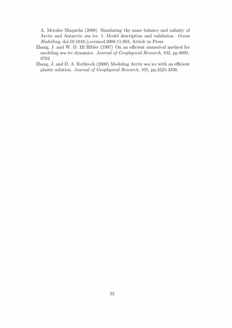
(41)respectively. For the LIM applications to be discussed below, the ratio ofplastic deformation radius to grid size, λ/d, lies between 2 and 3. From Fig.2, which displays contours of normalised frequency σ/f as a function of kdand ld for the case λ/d = 2, it is easy to see that the latter dispersion relationis closer to the exact relation, (38), than the former. In particular, on the C

12

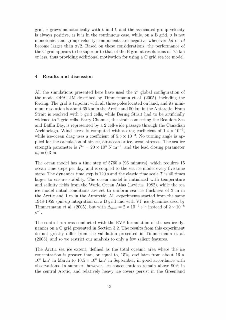
grid, σ grows monotonically with k and l, and the associated group velocityis always positive, as it is in the continuous case, while, on a B grid, σ is notmonotonic, and group velocity components are negative whenever kd or ldbecome larger than π/2. Based on these considerations, the performance ofthe C grid appears to be superior to that of the B grid at resolutions of 75 kmor less, thus providing additional motivation for using a C grid sea ice model.

4 Results and discussion

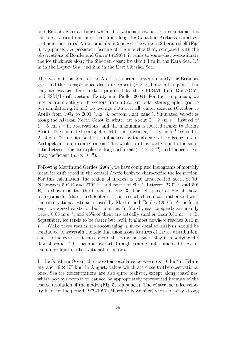
All the simulations presented here have used the 2◦ global configuration ofthe model OPA-LIM described by Timmermann et al. (2005), including theforcing. The grid is tripolar, with all three poles located on land, and its mini-mum resolution is about 65 km in the Arctic and 50 km in the Antarctic. FramStrait is resolved with 5 grid cells, while Bering Strait had to be artificiallywidened to 2 grid cells. Parry Channel, the strait connecting the Beaufort Seaand Baffin Bay, is represented by a 2 cell-wide passage through the CanadianArchipelago. Wind stress is computed with a drag coefficient of 1.4 × 10−3,while ice-ocean drag uses a coefficient of 5.5 × 10−3. No turning angle is ap-plied for the calculation of air-ice, air-ocean or ice-ocean stresses. The sea icestrength parameter is P ∗ = 20 × 103 N m−2, and the lead closing parameterh0 = 0.3 m.

The ocean model has a time step of 5760 s (96 minutes), which requires 15ocean time steps per day, and is coupled to the sea ice model every five timesteps. The dynamics time step is 120 s and the elastic time scale T is 40 timeslarger to ensure stability. The ocean model is initialized with temperatureand salinity fields from the World Ocean Atlas (Levitus, 1982), while the seaice model initial conditions are set to uniform sea ice thickness of 3 m inthe Arctic and 1 m in the Antarctic. All experiments started from the same1948-1959 spin-up integration on a B grid and with VP ice dynamics used byTimmermann et al. (2005), but with ∆min = 2× 10−9 s−1 instead of 2× 10−8

s−1.

The control run was conducted with the EVP formulation of the sea ice dy-namics on a C grid presented in Section 3.2. The results from this experimentdo not greatly differ from the validation presented in Timmermann et al.(2005), and so we restrict our analysis to only a few salient features.

The Arctic sea ice extent, defined as the total oceanic area where the iceconcentration is greater than, or equal to, 15%, oscillates from about 16 ×106 km2 in March to 10.5 × 106 km2 in September, in good accordance withobservations. In summer, however, ice concentrations remain above 90% inthe central Arctic, and relatively heavy ice covers persist in the Greenland

13

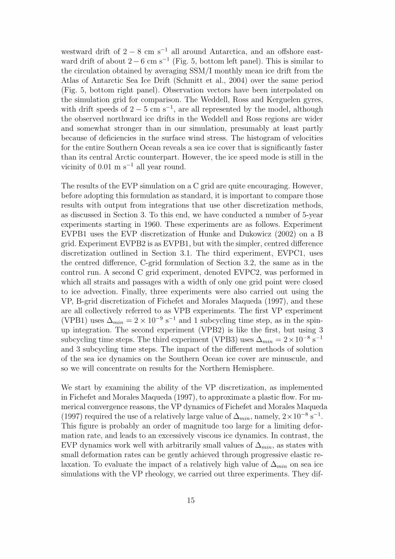
and Barents Seas at times when observations show ice-free conditions. Icethickness varies from more than 6 m along the Canadian Arctic Archipelagoto 4 m in the central Arctic, and about 2 m over the western Siberian shelf (Fig.3, top panels). A persistent feature of the model is that, compared with theobservations of Bourke and Garrett (1987), it tends to somewhat overestimatethe ice thickness along the Siberian coast: by about 1 m in the Kara Sea, 1.5m in the Laptev Sea, and 2 m in the East Siberian Sea.

The two main patterns of the Arctic ice current system, namely the Beaufortgyre and the transpolar ice drift are present (Fig. 3, bottom left panel) butthey are weaker than in data produced by the CERSAT from QuikSCATand SSM/I drift vectors (Ezraty and Piolle, 2004). For the comparison, weinterpolate monthly drift vectors from a 62.5 km polar stereographic grid toour simulation grid and we average data over all winter seasons (October toApril) from 1992 to 2001 (Fig. 3, bottom right panel). Simulated velocitiesalong the Alaskan North Coast in winter are about 0 − 2 cm s−1 instead of1 − 5 cm s−1 in observations, and the maximum is located nearer to BeringStrait. The simulated transpolar drift is also weaker, 1 − 3 cm s−1 instead of2−4 cm s−1, and its location is influenced by the absence of the Franz JosephArchipelago in our configuration. This weaker drift is partly due to the smallratio between the atmospheric drag coefficient (1.4× 10−3) and the ice-oceandrag coefficient (5.5 × 10−3).

Following Martin and Gerdes (2007), we have computed histograms of monthlymean ice drift speed in the central Arctic basin to characterise the ice motion.For this calculation, the region of interest is the area located north of 70◦

N between 50◦ E and 270◦ E, and north of 80◦ N between 270◦ E and 50◦

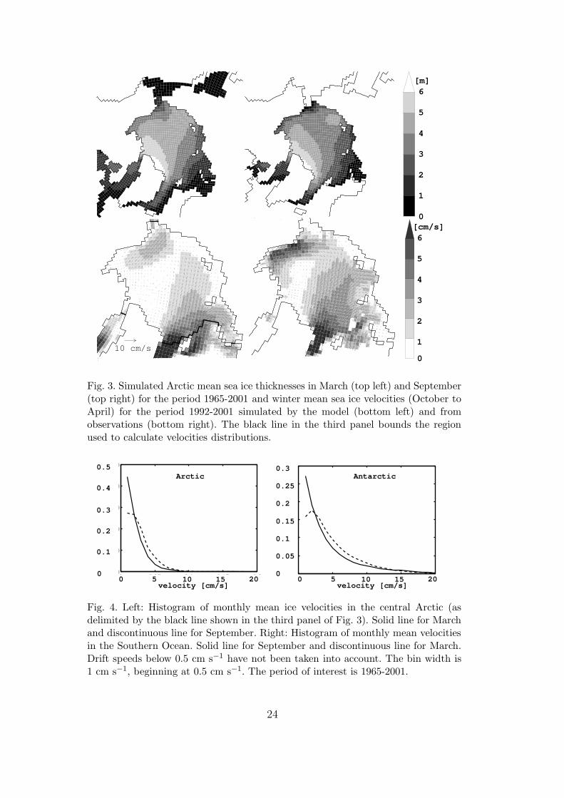
E, as shown on the third panel of Fig. 3. The left panel of Fig. 4 showshistograms for March and September, both of which compare rather well withthe observational estimates used by Martin and Gerdes (2007). A mode atvery low speed exists for both months. In March, sea ice speeds are mainlybelow 0.05 m s−1, and 45% of them are actually smaller than 0.01 m −1s. InSeptember, ice tends to be faster but, still, it almost nowhere reaches 0.10 ms−1. While these results are encouraging, a more detailed analysis should beconducted to ascertain the role that anomalous features of the ice distribution,such as the excess thickness along the Eurasian coast, play in modifying theflow of sea ice. The mean ice export through Fram Strait is about 0.11 Sv, inthe upper limit of observational estimates.

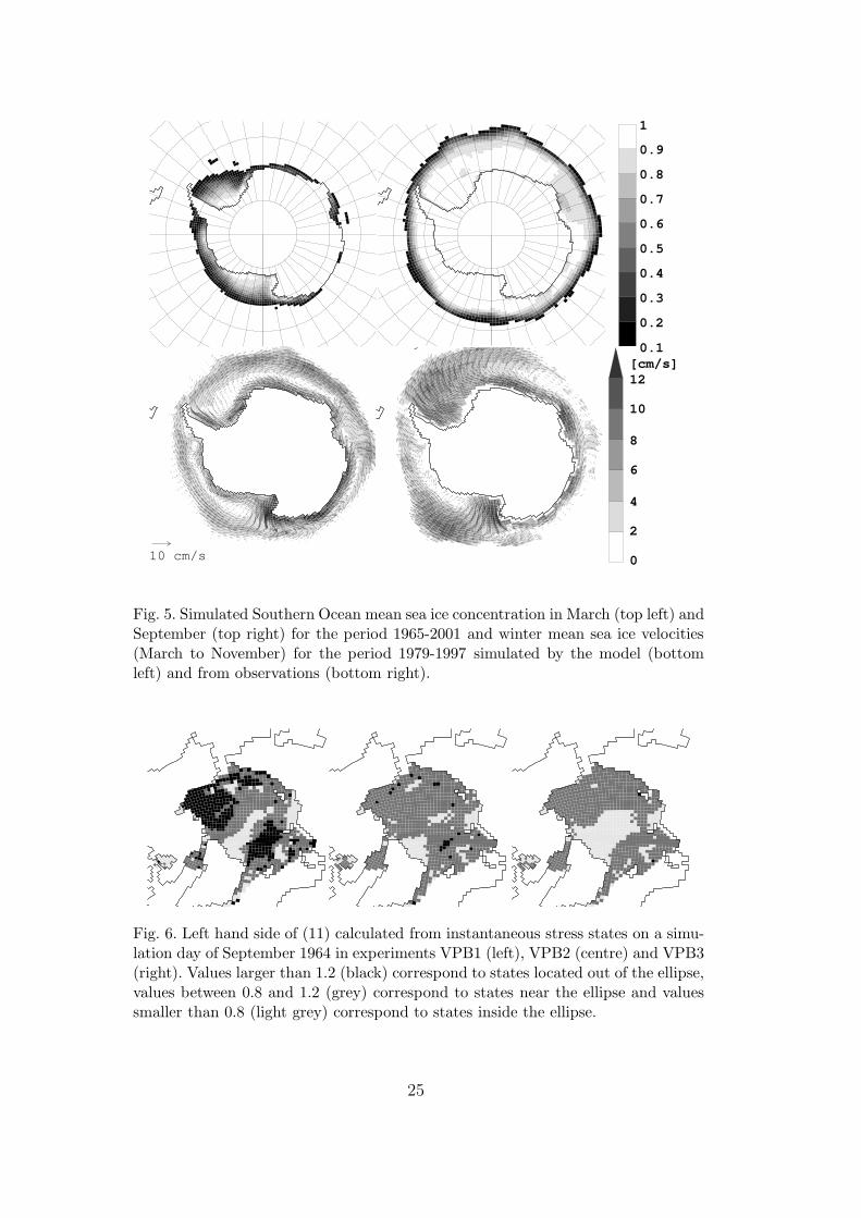
In the Southern Ocean, the ice extent oscillates between 5×106 km2 in Febru-ary and 19 × 106 km2 in August, values which are close to the observationalones. Sea ice concentrations are also quite realistic, except along coastlines,where polynya formation cannot be appropriately represented because of thecoarse resolution of the model (Fig. 5, top panels). The winter mean ice veloc-ity field for the period 1979-1997 (March to November) shows a fairly strong

14

westward drift of 2 − 8 cm s−1 all around Antarctica, and an offshore east-ward drift of about 2− 6 cm s−1 (Fig. 5, bottom left panel). This is similar tothe circulation obtained by averaging SSM/I monthly mean ice drift from theAtlas of Antarctic Sea Ice Drift (Schmitt et al., 2004) over the same period(Fig. 5, bottom right panel). Observation vectors have been interpolated onthe simulation grid for comparison. The Weddell, Ross and Kerguelen gyres,with drift speeds of 2 − 5 cm s−1, are all represented by the model, althoughthe observed northward ice drifts in the Weddell and Ross regions are widerand somewhat stronger than in our simulation, presumably at least partlybecause of deficiencies in the surface wind stress. The histogram of velocitiesfor the entire Southern Ocean reveals a sea ice cover that is significantly fasterthan its central Arctic counterpart. However, the ice speed mode is still in thevicinity of 0.01 m s−1 all year round.

The results of the EVP simulation on a C grid are quite encouraging. However,before adopting this formulation as standard, it is important to compare thoseresults with output from integrations that use other discretization methods,as discussed in Section 3. To this end, we have conducted a number of 5-yearexperiments starting in 1960. These experiments are as follows. ExperimentEVPB1 uses the EVP discretization of Hunke and Dukowicz (2002) on a Bgrid. Experiment EVPB2 is as EVPB1, but with the simpler, centred differencediscretization outlined in Section 3.1. The third experiment, EVPC1, usesthe centred difference, C-grid formulation of Section 3.2, the same as in thecontrol run. A second C grid experiment, denoted EVPC2, was performed inwhich all straits and passages with a width of only one grid point were closedto ice advection. Finally, three experiments were also carried out using theVP, B-grid discretization of Fichefet and Morales Maqueda (1997), and theseare all collectively referred to as VPB experiments. The first VP experiment(VPB1) uses ∆min = 2 × 10−9 s−1 and 1 subcycling time step, as in the spin-up integration. The second experiment (VPB2) is like the first, but using 3subcycling time steps. The third experiment (VPB3) uses ∆min = 2×10−8 s−1

and 3 subcycling time steps. The impact of the different methods of solutionof the sea ice dynamics on the Southern Ocean ice cover are minuscule, andso we will concentrate on results for the Northern Hemisphere.

We start by examining the ability of the VP discretization, as implementedin Fichefet and Morales Maqueda (1997), to approximate a plastic flow. For nu-merical convergence reasons, the VP dynamics of Fichefet and Morales Maqueda(1997) required the use of a relatively large value of ∆min, namely, 2×10−8 s−1.This figure is probably an order of magnitude too large for a limiting defor-mation rate, and leads to an excessively viscous ice dynamics. In contrast, theEVP dynamics work well with arbitrarily small values of ∆min, as states withsmall deformation rates can be gently achieved through progressive elastic re-laxation. To evaluate the impact of a relatively high value of ∆min on sea icesimulations with the VP rheology, we carried out three experiments. They dif-

15

fer in the minimum value of ∆min used and also in the number of subcyclingtime steps for the dynamics (subcycling consists in solving the momentumequation with a time step smaller than the one used for ice thermodynamicsand transport).

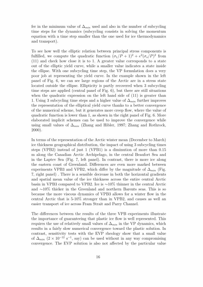
To see how well the elliptic relation between principal stress components isfulfilled, we compute the quadratic function (σ1/P + 1)2 + e2(σs/P )2 from(11) and check how close it is to 1. A greater value corresponds to a stateout of the elliptic yield curve, while a smaller value indicates a state insidethe ellipse. With one subcycling time step, the VP formulation does a verypoor job at representing the yield curve. In the example shown in the leftpanel of Fig. 6, we can see large regions of the Arctic are in a stress statelocated outside the ellipse. Ellipticity is partly recovered when 3 subcyclingtime steps are applied (central panel of Fig. 6), but there are still situationswhen the quadratic expression on the left hand side of (11) is greater than1. Using 3 subcycling time steps and a higher value of ∆min further improvesthe representation of the elliptical yield curve thanks to a better convergenceof the numerical scheme, but it generates more creep flow, where the value ofquadratic function is lower than 1, as shown in the right panel of Fig. 6. Moreelaborated implicit schemes can be used to improve the convergence whileusing small values of ∆min (Zhang and Hibler, 1997; Zhang and Rothrock,2000).

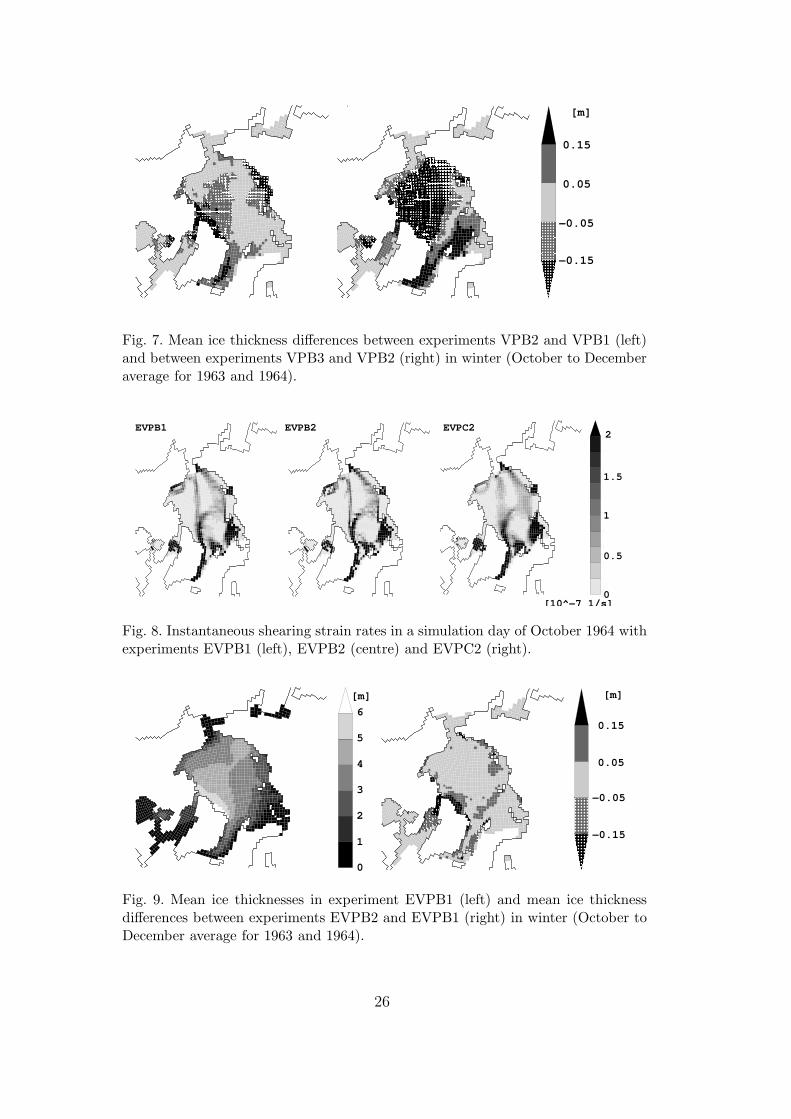
In terms of the representation of the Arctic winter mean (December to March)ice thickness geographical distribution, the impact of using 3 subcycling timessteps (VPB2) instead of just 1 (VPB1) is a diminution of more than 0.15m along the Canadian Arctic Archipelago, in the central Beaufort Sea andin the Laptev Sea (Fig. 7, left panel). In contrast, there is more ice alongthe eastern coast of Greenland. Differences are even more marked betweenexperiments VPB3 and VPB2, which differ by the magnitude of ∆min (Fig.7, right panel) . There is a sensible decrease in both the horizontal gradientsand spatial mean value of the ice thickness across the entire central Arcticbasin in VPB3 compared to VPB2. Ice is ∼10% thinner in the central Arcticand ∼10% thicker in the Greenland and northern Barents seas. This is sobecause the more viscous dynamics of VPB3 allows for a winter flow in thecentral Arctic that is 5-10% stronger than in VPB2, and causes as well aneasier transport of ice across Fram Strait and Parry Channel.

The differences between the results of the three VPB experiments illustratethe importance of guaranteeing that plastic ice flow is well represented. Thisrequires the use of relatively small values of ∆min in the VP dynamics, whichresults in a fairly slow numerical convergence toward the plastic solution. Incontrast, sensitivity tests with the EVP rheology show that a small valueof ∆min (2 × 10−12 s−1, say) can be used without in any way compromisingconvergence. The EVP solution is also not affected by the particular value

16

of T chosen, as long as it is several times smaller than the thermodynamicsand transport time steps. Thus, with suitable ∆min and T values, ice internalstress states calculated with the EVP formulation tend to be much closer tothe elliptical yield curve than those determined using the VP rheology.

The aim of experiments EVPB1, EVPB2, EVPC1 and EVPC2 was to examinethe influence of the spatial discretization on EVP solutions. Overall, there isa reassuring similarity between the results of all four experiments, althoughwe note that the B grid tends to develop checkerboard patterns in certainvariables, such as the ice divergence field. In most cases, this computationalmode does not appear to have a direct impact on the ice dynamics, but itcould be a problem if deformation rates are used in the calculation of theice thickness redistribution. The use of a bilinear approach a la Hunke andDukowicz (2002), rather than the more simple centred difference formulationwe have proposed in Section 3.1, helps attenuating the checkerboard modethanks to the spatial averaging involved in the calculation of the internalstress force. This numerical mode cannot appear on a C grid.

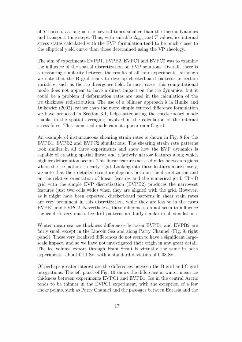
An example of instantaneous shearing strain rates is shown in Fig. 8 for theEVPB1, EVPB2 and EVPC2 simulations. The shearing strain rate patternslook similar in all three experiments and show how the EVP dynamics iscapable of creating spatial linear and relatively narrow features along whichhigh ice deformation occurs. This linear features act as divides between regionswhere the ice motion is nearly rigid. Looking into these features more closely,we note that their detailed structure depends both on the discretization andon the relative orientation of linear features and the numerical grid. The Bgrid with the simple EVP discretization (EVPB2) produces the narrowestfeatures (just two cells wide) when they are aligned with the grid. However,as it might have been expected, checkerboard patterns in shear stain ratesare very prominent in this discretization, while they are less so in the casesEVPB1 and EVPC2. Nevertheless, these differences do not seem to influencethe ice drift very much. Ice drift patterns are fairly similar in all simulations.

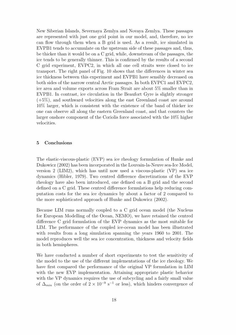
Winter mean sea ice thickness differences between EVPB1 and EVPB2 arefairly small except in the Lincoln Sea and along Parry Channel (Fig. 9, rightpanel). These very localized differences do not seem to have a significant large-scale impact, and so we have not investigated their origin in any great detail.The ice volume export through Fram Strait is virtually the same in bothexperiments: about 0.11 Sv, with a standard deviation of 0.08 Sv.

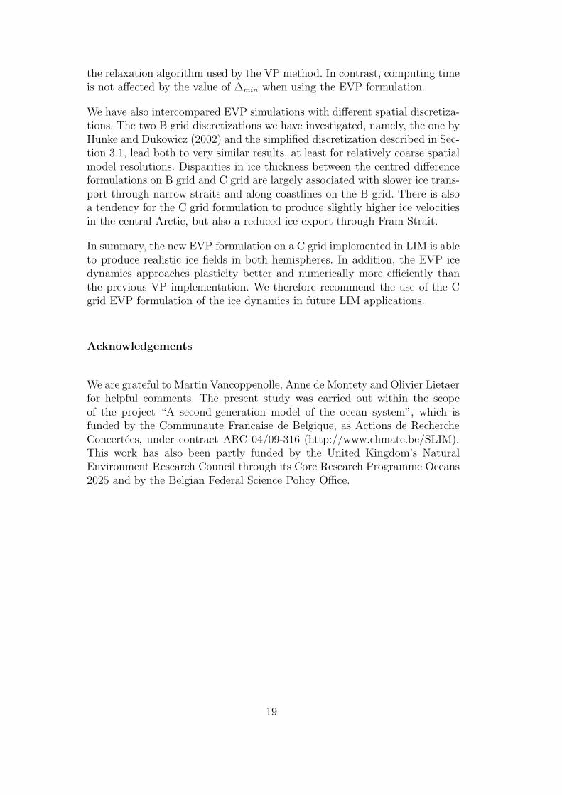
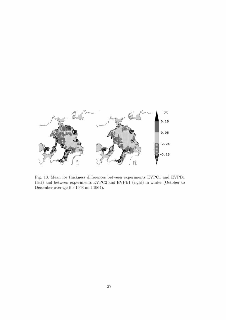
Of perhaps greater interest are the differences between the B grid and C gridintegrations. The left panel of Fig. 10 shows the difference in winter mean icethickness between experiments EVPC1 and EVPB1. Ice in the central Arctictends to be thinner in the EVPC1 experiment, with the exception of a fewchoke points, such as Parry Channel and the passages between Eurasia and the

17

New Siberian Islands, Severnaya Zemlya and Novaya Zemlya. These passagesare represented with just one grid point in our model, and, therefore, no icecan flow through them when a B grid is used. As a result, ice simulated inEVPB1 tends to accumulate on the upstream side of these passages and, thus,be thicker than it would be on a C grid, while, downstream of the passages, theice tends to be generally thinner. This is confirmed by the results of a secondC grid experiment, EVPC2, in which all one cell straits were closed to icetransport. The right panel of Fig. 10 shows that the differences in winter seaice thickness between this experiment and EVPB1 have sensibly decreased onboth sides of the narrow central Arctic passages. In both EVPC1 and EVPC2,ice area and volume exports across Fram Strait are about 5% smaller than inEVPB1. In contrast, ice circulation in the Beaufort Gyre is slightly stronger(+5%), and southward velocities along the east Greenland coast are around10% larger, which is consistent with the existence of the band of thicker iceone can observe all along the eastern Greenland coast, and that counters thelarger onshore component of the Coriolis force associated with the 10% highervelocities.

5 Conclusions

The elastic-viscous-plastic (EVP) sea ice rheology formulation of Hunke andDukowicz (2002) has been incorporated in the Louvain-la-Neuve sea-Ice Model,version 2 (LIM2), which has until now used a viscous-plastic (VP) sea icedynamics (Hibler, 1979). Two centred difference discretizations of the EVPrheology have also been introduced, one defined on a B grid and the seconddefined on a C grid. These centred difference formulations help reducing com-putation costs for the sea ice dynamics by about a factor of 2 compared tothe more sophisticated approach of Hunke and Dukowicz (2002).

Because LIM runs normally coupled to a C grid ocean model (the Nucleusfor European Modelling of the Ocean, NEMO), we have retained the centreddifference C grid formulation of the EVP dynamics as the most suitable forLIM. The performance of the coupled ice-ocean model has been illustratedwith results from a long simulation spanning the years 1960 to 2001. Themodel reproduces well the sea ice concentration, thickness and velocity fieldsin both hemispheres.

We have conducted a number of short experiments to test the sensitivity ofthe model to the use of the different implementations of the ice rheology. Wehave first compared the performance of the original VP formulation in LIMwith the new EVP implementation. Attaining appropriate plastic behaviorwith the VP dynamics requires the use of subcycling and a fairly small valueof ∆min (on the order of 2 × 10−9 s−1 or less), which hinders convergence of

18

the relaxation algorithm used by the VP method. In contrast, computing timeis not affected by the value of ∆min when using the EVP formulation.

We have also intercompared EVP simulations with different spatial discretiza-tions. The two B grid discretizations we have investigated, namely, the one byHunke and Dukowicz (2002) and the simplified discretization described in Sec-tion 3.1, lead both to very similar results, at least for relatively coarse spatialmodel resolutions. Disparities in ice thickness between the centred differenceformulations on B grid and C grid are largely associated with slower ice trans-port through narrow straits and along coastlines on the B grid. There is alsoa tendency for the C grid formulation to produce slightly higher ice velocitiesin the central Arctic, but also a reduced ice export through Fram Strait.

In summary, the new EVP formulation on a C grid implemented in LIM is ableto produce realistic ice fields in both hemispheres. In addition, the EVP icedynamics approaches plasticity better and numerically more efficiently thanthe previous VP implementation. We therefore recommend the use of the Cgrid EVP formulation of the ice dynamics in future LIM applications.

Acknowledgements

We are grateful to Martin Vancoppenolle, Anne de Montety and Olivier Lietaerfor helpful comments. The present study was carried out within the scopeof the project “A second-generation model of the ocean system”, which isfunded by the Communaute Francaise de Belgique, as Actions de RechercheConcertees, under contract ARC 04/09-316 (http://www.climate.be/SLIM).This work has also been partly funded by the United Kingdom’s NaturalEnvironment Research Council through its Core Research Programme Oceans2025 and by the Belgian Federal Science Policy Office.

19

References

Bourke, R. H. and R. P. Garrett (1987) Sea ice thickness distribution in theArctic Ocean. Cold Regions Science and Technology, 13, pp.259-280.

Connolley, W. M., J. M. Gregory, E. Hunke and A. J. McLaren (2004) Onthe consistent scaling of terms in the sea-ice dynamics equation. Journal of

Physical Oceanography, 34(7), pp.1776-1780.Driesschaert, E., T. Fichefet, H. Goosse, P. Huybrechts, I. Janssens, A.

Mouchet, G. Munhoven, V. Brovkin, and S.L. Weber (2007) Model-ing the influence of Greenland ice sheet melting on the Atlantic merid-ional overturning circulation. Geophysical Research Letters, 34, L10707,doi:10.1029/2007GL029516.

Ezraty, R. and J.F. Piolle (2004) Sea-ice drift in the central Arctic combiningQuikSCAT and SSM/I sea ice drift data - User’s manual (v1.0, April 2004)Available at ftp://ftp.ifremer.fr/ifremer/cersat/products/gridded/psi-drift/documentation/merged.pdf

Fichefet, T. and M. A. Morales Maqueda (1997) Sensitivity of a global seaice model to the treatment of ice thermodynamics and dynamics. Journal

of Geophysical Research, 102, pp.12609-12646.Fichefet, T. and M. A. Morales Maqueda (1999) Modelling the influence of

snow accumulation and snow-ice formation on the seasonal cycle of theantarctic sea-ice cover. Climate Dynamics, 15, pp.251-268.

Flato, G. M. and W. D. Hibler (1992) Modeling pack ice as a cavitating fluid.Journal of Physical Oceanography, 22, pp.626-651.

Goosse, H. (1997) Modelling the large-scale behaviour of the coupled ocean-sea ice system. Ph. D. thesis, 231 pp., Fac. des Sci. Appl. Univ. Cath. deLouvain, Louvain-la-Neuve, Belgium.

Goosse, H. and T. Fichefet (1999) Importance of ice-ocean interactions for theglobal ocean circulation: A model study. Journal of Geophysical Research,104, pp.23337-23355.

Gray, J. M. N. T. (1999) Loss of hyperbolocity and ill-posedness of the viscous-plastic sea ice rheology in uniaxial divergent flow. Journal of Physical

Oceanography, 29(11), pp.2920-2929.Hibler, W. D. III (1979) A dynamic thermodynamic sea ice model. Journal

of Physical Oceanography, 9, pp.817-846.Hofmann, M. and M. A. Morales Maqueda (2006) Performance of a second-

order moment advection scheme in an ocean general circulation model. Jour-

nal of Geophysical Research, 111, pp.C05006, doi:10.1029/2005JC003279.Hunke, E. C. and J. K. Dukowicz (1997) An elastic-viscous-plastic model for

sea ice dynamics. Journal of Physical Oceanography, 27, pp.1849-1867.Hunke, E. C. and J. K. Dukowicz (2002) The elastic-viscous-plastic sea ice

dynamics model in general orthogonal curvilinear coordinates on a sphere-incorporation of metric terms. Monthly Weather Review, 130, pp.1848-1865.

Hunke, E. C. and W. H. Lipscomb (2006) CICE: the Los Alamos Sea IceModel Documentation and Software User’s Manual, Tech. Report LA-CC-

20

98-16, 59 pp., T-3 Fluid Dynamics Group, Los Alamos National Laboratory,Los Alamos NM 87545.

Hunke, E. C. and Y. Zhang (1999) A Comparison of sea ice dynamics modelsat high resolution Monthly Weather Review, 127, pp.396-408.

Kantha, L. H. and C. A. Clayson (2000) Numerical Models of Oceans andOceanic Processes. Academic Press, ISBN 012 4340687, 940 pp.

Lepparanta, M. (2005) The Drift of Sea Ice. Springer, Helsinki, 266pp.Levitus, S. (1982) Climatological atlas of the world ocean. NOAA Professional

Paper 13, US Government Printing Office, Washington DC.Madec, G., P. Delecluse, M. Imbard and C. Lvy (1999) OPA 8.1, Ocean

general circulation model reference manual. Laboratoire d’OcanographieDynamique et de Climatologie, Paris, France.

Marti O., P. Braconnot, J.-L. Dufresne, J. Bellier, R. Benshila, S. Bony, P.Brockmann, P. Cadule, A. Caubel, F. Codron, N. de Noblet, S. Denvil,L. Fairhead, T. Fichefet, M.-A. Foujols, P. Friedlingstein, H. Goosse, J.-Y.Grandpeix, E. Guilyardi, F. Hourdin, G. Krinner, C. Lvy, G. Madec, J.Mignot, I. Musat, D. Swingedouw, and C. Talandier (2008) Key featuresof the IPSL ocean atmosphere model and its sensitivity to atmosphericresolution. Climate Dynamics, submitted.

Martin, T. and R. Gerdes (2007) Sea ice drift variability in Arctic Ocean ModelIntercomparison Project models and observations. Journal of Geophysical

Research, 112, pp.C04S10, doi:10.1029/2006JC003617.McPhee, M. G. (1992) Turbulent heat fluxes in the upper ocean under sea

ice. Journal of Geophysical Research, 97, pp.5365-5379.Montoya, M., A. Griesel, A. Levermann, J. Mignot, M. Hofmann, A. Ganopol-

ski and S. Rahmstorf (2005) The earth system model of intermediate com-plexity CLIMBER-3α. Part I: description and performance for present-dayconditions. Climate Dynamics, 26, pp.237-263.

Randall, D. A. (1994) Geostrophic adjustment and the finite-differenceshallow-water equations. Monthly Weather Review, 122, pp.1371-1377.

Randall, D. A., R.A. Wood, S. Bony, R. Colman, T. Fichefet, J. Fyfe, V.Kattsov, A. Pitman, J. Shukla, J. Srinivasan, R.J. Stouffer, A. Sumi andK.E. Taylor (2007) Climate Models and Their Evaluation. In: ClimateChange 2007: The Physical Science Basis. Contribution of Working Group Ito the Fourth Assessment Report of the Intergovernmental Panel on ClimateChange [Solomon, S., D. Qin, M. Manning, Z. Chen, M. Marquis, K.B.Averyt, M.Tignor and H.L. Miller (eds.)]. Cambridge University Press,Cambridge, United Kingdom and New York, NY, USA.

Schmitt, C., Ch. Kottmeier, S. Wassermann and M. Drinkwater (2004)Atlas of Antarctic Sea Ice Drift. Available at http://www.imk.uni-karlsruhe.de/seaiceatlas

Timmermann, R., H. Goosse, G. Madec, T. Fichefet, C. Ethe, and V. Dulire(2005) On the representation of high latitude processes in the orca-limglobal coupled sea ice-ocean model. Ocean Modelling, 8, pp.175-201.

Vancoppenolle, M., T. Fichefet, H. Goosse, S. Bouillon, G. Madec and M.

21

A. Morales Maqueda (2008) Simulating the mass balance and salinity ofArctic and Antarctic sea ice. 1. Model description and validation. Ocean

Modelling, doi:10.1016/j.ocemod.2008.11.003, Article in Press.Zhang, J. and W. D. III Hibler (1997) On an efficient numerical method for

modeling sea ice dynamics. Journal of Geophysical Research, 102, pp.8691-8702.

Zhang, J. and D. A. Rothrock (2000) Modeling Arctic sea ice with an efficientplastic solution. Journal of Geophysical Research, 105, pp.3325-3338.

22

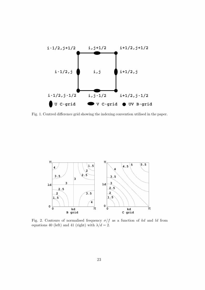
Fig. 1. Centred difference grid showing the indexing convention utilised in the paper.

1.5

2

2.5

3

0

3.5

4

00

5.55

1.5

2

2.5

3

3.5

44.51.5

2.5

2

3.5

4

3

π

B grid C gridkd kd

ld

0

ld

π

π π

Fig. 2. Contours of normalised frequency σ/f as a function of kd and ld fromequations 40 (left) and 41 (right) with λ/d = 2.

23

6

5

4

3

2

1

0

[m]

6

5

4

3

2

1

[cm/s]

010 cm/s

Fig. 3. Simulated Arctic mean sea ice thicknesses in March (top left) and September(top right) for the period 1965-2001 and winter mean sea ice velocities (October toApril) for the period 1992-2001 simulated by the model (bottom left) and fromobservations (bottom right). The black line in the third panel bounds the regionused to calculate velocities distributions.

0 0.05 0.1 0.15 0.20

10

20

30

40

50

|u| [m/s]

%

0 0.05 0.1 0.15 0.20

5

10

15

20

25

30

|u| [m/s]

%

0 0.05 0.1 0.15 0.20

10

20

30

40

50

|u| [m/s]

%

20151050201510500

0.1

0.2

0.3

0.4

0.5

velocity [cm/s]

0.25

0.2

0.15

0.1

0.3

0

0.05

velocity [cm/s]

Arctic Antarctic

Fig. 4. Left: Histogram of monthly mean ice velocities in the central Arctic (asdelimited by the black line shown in the third panel of Fig. 3). Solid line for Marchand discontinuous line for September. Right: Histogram of monthly mean velocitiesin the Southern Ocean. Solid line for September and discontinuous line for March.Drift speeds below 0.5 cm s−1 have not been taken into account. The bin width is1 cm s−1, beginning at 0.5 cm s−1. The period of interest is 1965-2001.

24

10

8

6

4

2

0

[cm/s]0.1

0.2

0.3

0.4

0.5

0.6

0.7

0.8

0.9

1

12

10 cm/s

Fig. 5. Simulated Southern Ocean mean sea ice concentration in March (top left) andSeptember (top right) for the period 1965-2001 and winter mean sea ice velocities(March to November) for the period 1979-1997 simulated by the model (bottomleft) and from observations (bottom right).

Fig. 6. Left hand side of (11) calculated from instantaneous stress states on a simu-lation day of September 1964 in experiments VPB1 (left), VPB2 (centre) and VPB3(right). Values larger than 1.2 (black) correspond to states located out of the ellipse,values between 0.8 and 1.2 (grey) correspond to states near the ellipse and valuessmaller than 0.8 (light grey) correspond to states inside the ellipse.

25

[m]

−0.15

−0.05

0.15

0.05

Fig. 7. Mean ice thickness differences between experiments VPB2 and VPB1 (left)and between experiments VPB3 and VPB2 (right) in winter (October to Decemberaverage for 1963 and 1964).

[10^−7 1/s]

EVPB1 EVPB2 EVPC2

1

1.5

0.5

0

2

Fig. 8. Instantaneous shearing strain rates in a simulation day of October 1964 withexperiments EVPB1 (left), EVPB2 (centre) and EVPC2 (right).

5

4

3

2

1

0

6

[m] [m]

0.15

0.05

−0.05

−0.15

Fig. 9. Mean ice thicknesses in experiment EVPB1 (left) and mean ice thicknessdifferences between experiments EVPB2 and EVPB1 (right) in winter (October toDecember average for 1963 and 1964).

26

[m]

−0.15

−0.05

0.15

0.05

Fig. 10. Mean ice thickness differences between experiments EVPC1 and EVPB1(left) and between experiments EVPC2 and EVPB1 (right) in winter (October toDecember average for 1963 and 1964).

27