AN EFFICIENT EQUATION GENERATION MECHANISM...
69
AN EFFICIENT EQUATION GENERATION MECHANISM FOR A COMPONENT-BASED MODELING SCHEME By Aparna Barve Thesis Submitted to the Faculty of the Graduate School of Vanderbilt University in partial fulfillment of the requirements for the degree of MASTER OF SCIENCE in Computer Science May, 2008 Nashville, Tennessee Approved: Professor Gautam Biswas Professor Xenofon Koutsoukos
Transcript of AN EFFICIENT EQUATION GENERATION MECHANISM...

AN EFFICIENT EQUATION GENERATION MECHANISM FOR A
COMPONENT-BASED MODELING SCHEME
By
Aparna Barve
Thesis
Submitted to the Faculty of the
Graduate School of Vanderbilt University
in partial fulfillment of the requirements
for the degree of
MASTER OF SCIENCE
in
Computer Science
May, 2008
Nashville, Tennessee
Approved:
Professor Gautam Biswas
Professor Xenofon Koutsoukos

This thesis is dedicated to my parents, Archana and Ashok Barve.
ii

ACKNOWLEDGEMENTS
I would like to thank my advisor, Dr. Gautam Biswas, for providing valuable guid-
ance during the course of my Masters research and for his insightful comments. I am
grateful to my secondary advisor Dr. Xenofon Koutsoukos for his constructive feed-
back. I would also like to thank Mr. Nag Mahadevan for his timely suggestions and
valuable inputs in working out the implementation details for my thesis. I appreciate
all the help provided to me by my fellow graduate students at Vanderbilt University
and at the Institute of Software Integrated Systems.
Last but not the least, I would like to acknowledge the support and encouragement
provided by my family during my Masters studies.
iii

TABLE OF CONTENTS
Page
LIST OF TABLES . . . . . . . . . . . . . . . . . . . . . . . . . . . . . . . . . vi
LIST OF FIGURES . . . . . . . . . . . . . . . . . . . . . . . . . . . . . . . . vii
Chapter
I. INTRODUCTION . . . . . . . . . . . . . . . . . . . . . . . . . . . . 1
I.1. Main Contributions . . . . . . . . . . . . . . . . . . . . . . . 2I.2. Organization of Thesis . . . . . . . . . . . . . . . . . . . . . 3
II. BUILDING OBSERVERS FROM BOND GRAPH MODELS . . . . 4
II.1. Bond Graph Modeling Language . . . . . . . . . . . . . . . 4II.2. Causality in Bond Graphs . . . . . . . . . . . . . . . . . . . 5II.3. Generating Mathematical Models from BG . . . . . . . . . . 6II.4. Building Kalman Filters . . . . . . . . . . . . . . . . . . . . 7
III. IMPLEMENTING KALMAN FILTERS FROM BOND GRAPH MODEL 9
III.1. Modeling Environment . . . . . . . . . . . . . . . . . . . . . 9III.1.1. Introduction to FACT . . . . . . . . . . . . . . . . 9III.1.2. Extensions for n-port elements . . . . . . . . . . . . 10
III.2. Efficient methods for generating State Space Models . . . . 13III.2.1. Data Structures . . . . . . . . . . . . . . . . . . . . 14III.2.2. State Equation Generation Algorithm . . . . . . . . 26III.2.3. Output Equation Generation Algorithm . . . . . . 30III.2.4. Basic Equation Generation Algorithm . . . . . . . . 30III.2.5. Extension for Transformers and Gyrators . . . . . . 31III.2.6. Extensions to SCAP . . . . . . . . . . . . . . . . . 35
III.3. Building the Kalman Filter . . . . . . . . . . . . . . . . . . 36
IV. EXPERIMENTAL RESULTS . . . . . . . . . . . . . . . . . . . . . . 41
IV.1. Hydraulic Actuator System . . . . . . . . . . . . . . . . . . 41IV.1.1. Equation Generation for the Hydraulic Actuator Sys-
tem . . . . . . . . . . . . . . . . . . . . . . . . . . . 42IV.1.2. Observer runs with measurement noise and modeling
errors in the system model . . . . . . . . . . . . . . 43IV.2. N-port system . . . . . . . . . . . . . . . . . . . . . . . . . . 54
iv

V. CONCLUSIONS . . . . . . . . . . . . . . . . . . . . . . . . . . . . . 59
V.1. Future Work . . . . . . . . . . . . . . . . . . . . . . . . . . 59
BIBLIOGRAPHY . . . . . . . . . . . . . . . . . . . . . . . . . . . . . . . . . 60
v

LIST OF TABLES
Table Page
IV.1. Description of the Actuator Parameters . . . . . . . . . . . . . . . . . . . 42
IV.2. Mean Square Error Values . . . . . . . . . . . . . . . . . . . . . . . . . 51
vi

LIST OF FIGURES
Figure Page
I.1. TRANSCEND System Architecture . . . . . . . . . . . . . . . . . . 2
II.1. Model Based Diagnosis . . . . . . . . . . . . . . . . . . . . . . . . . 7
III.1. Bond Graph Elements Class Hierarchy . . . . . . . . . . . . . . . . 11
III.2. Class Hierarchy for N-port Elements . . . . . . . . . . . . . . . . . 12
III.3. Constraints for N-port Elements . . . . . . . . . . . . . . . . . . . 13
III.4. Schematic Diagram of a Two Tank System . . . . . . . . . . . . . . 14
III.5. Fixed and Multi-port Variable Causality Assignments and BD rep-resentation . . . . . . . . . . . . . . . . . . . . . . . . . . . . . . . 15
III.6. 1- and 2-port Variable Causality Assignments and BD representation 16
III.7. A GME Bond Graph Model of a Two Tank System . . . . . . . . 16
III.8. A Block Diagram Model of a Two Tank System . . . . . . . . . . 17
III.9. Template of the Node Data Structure . . . . . . . . . . . . . . . . . 18
III.10. Algorithm for assigning Bond numbers . . . . . . . . . . . . . . . 24
III.11. Equation Generation trace for state variable e5 . . . . . . . . . . . 28
III.12. Algorithm for generating State Space Equations . . . . . . . . . . 29
III.13. Basic Equation Generation Algorithm . . . . . . . . . . . . . . . . 34
III.14. Causal assignments and corresponding equations for a Transformer 34
III.15. Causal assignments and corresponding equations for a Gyrator . . . 35
III.16. Causality Assignment for nC and nI . . . . . . . . . . . . . . . . . 36
III.17. Kalman Filter Equations for Process and Measurement Model . . . 38
III.18. Observer and System Output for a Two Tank System . . . . . . . 39
vii

IV.1. A simplified model for the Hydraulic Actuator . . . . . . . . . . . . 41
IV.2. A GME Bond Graph Model of Hydraulic Actuator System . . . . 42
IV.3. Simulink Model of the Hydraulic Actuator System . . . . . . . . . 44
IV.4. Pressure Output of the Hydraulic Actuator System . . . . . . . . . 44
IV.5. A GME Bond Graph Model of a part of the Hydraulic ActuatorSystem . . . . . . . . . . . . . . . . . . . . . . . . . . . . . . . . . 45
IV.6. Measured and Observed values for Actuator for a measurement noiseof 2 percent . . . . . . . . . . . . . . . . . . . . . . . . . . . . . . . 48
IV.7. Measured and Observed values for Actuator for a measurement noiseof 5 percent . . . . . . . . . . . . . . . . . . . . . . . . . . . . . . . 49
IV.8. Measured and Observed values for Actuator for a measurement noiseof 8 percent . . . . . . . . . . . . . . . . . . . . . . . . . . . . . . . 50
IV.9. Measured and Observed values for Actuator for a measurement noiseof 2 percent, Se increased by 2 percent and R valve decreased by 2percent . . . . . . . . . . . . . . . . . . . . . . . . . . . . . . . . . 51
IV.10. Measured and Observed values for Actuator for a measurement noiseof 2 percent, Se decreased by 5 percent and R valve increased by 5percent . . . . . . . . . . . . . . . . . . . . . . . . . . . . . . . . . 52
IV.11. Measured and Observed values for Actuator for a measurement noiseof 8 percent, Se increased by 2 percent and R valve decreased by 8percent . . . . . . . . . . . . . . . . . . . . . . . . . . . . . . . . . 53
IV.12. Bond Graph model of the system with an n-port element . . . . . . 54
IV.13. Observer and System Output for a Two Tank System implementedusing nC . . . . . . . . . . . . . . . . . . . . . . . . . . . . . . . . 57
viii
CHAPTER I
INTRODUCTION
The thesis addresses the problem of building observers from component-based
models of continuous dynamic systems. We build models using bond graphs, which
provide a domain independent, energy-based, topological scheme for capturing the
dynamic behavior of physical systems [9]. The observer plays an important part in
online diagnosis schemes by providing reliable estimates of system state and system
output in the presence of noise in the measurements and discrepancies in the system
model. The estimated outputs are compared against the observed measurements to
compute the system residuals. Non-zero residuals imply faults in the system.
The TRANSCEND (TRANSient based Continuous ENgineering Diagnosis) [12]
provides such a model based system for monitoring and diagnosis of complex dynamic
systems. As shown in Fig. I.1, the observer tracks the residuals
r = y − y,
i.e. the difference between the actual and the predicted observations. A non-zero
residual triggers the fault diagnosis process.
We use the FACT [6] (Fault Adaptive Control Technology) system developed in
the Generic Modeling Environment for diagnosis applications. It allows us to build
component-oriented bond graph models of our systems and also provides a run time
environment for carrying out fault diagnosis.
The steps involved in building the observer involve transforming the component-
based bond graph model of the physical system to its corresponding block diagram
1

Figure I.1: TRANSCEND System Architecture
model and generating the state space equations and the output equations from this
model. The observer is implemented as a Kalman filter.
I.1 Main Contributions
A previous implementation [6] of the observer in the FACT system did not ex-
plicitly use the causality information from the bond graph while generating equations
for the system. Instead, it used a more brute force approach by generating equations
for every component in the bond graph model and manipulating them over multiple
iterations till all the equations could be represented in the state space form. This
method of manipulating the multiple equations fragments simultaneously made the
equation generation process inefficient and computationally complex. It was clear
that this complexity could be significantly reduced by exploiting the computational
causality of the bonds in the bond graphs [8].
The main contribution of the thesis is to implement an efficient equation gener-
ation mechanism for the component based modeling paradigm in FACT. Assigning
causalities to the bonds captures the cause effect relationship between the bond graph
2

elements and considering these causalities in the equation generation algorithm signif-
icantly simplifies the process of deriving the state and output equations of the system.
We use these models to construct a Kalman filter based observer to track continuous
system behavior for linear systems. We also provide a mechanism for extending the
modeling paradigm to include n-port elements that play an important part in the
modeling on multi-domain physical systems.
I.2 Organization of Thesis
The thesis is organized as follows.
Chapter II of the thesis provides a background of the various components involved
in designing state space observers, the Bond Graph Modeling Language, the concept
of causality, equation generation, and Kalman filters. Chapter III provides a detailed
overview of the implementation details, which includes the extensions made to the
modeling paradigm, the algorithms used for equation generation, followed by the
building of the Kalman filter from the generated equations. The simulation and the
experimental results are discussed in Chapter IV. Chapter V elaborates on the future
work and provides the conclusion for the thesis.
3

CHAPTER II
BUILDING OBSERVERS FROM BOND GRAPH
MODELS
This chapter gives a brief overview of the process of building observers from bond
graph models and presents a background for the problems addressed in the thesis.
An overview of the bond graph modeling language that is used to construct the input
models for our system is presented at the beginning of this chapter. In this chapter,
we also explain the concept of causality in bond graphs, followed by the process
of generating mathematical equations from the given bond graph models. Lastly,
we discuss Kalman filters and show how they can be built based on the generated
equations.
II.1 Bond Graph Modeling Language
The bond graph modeling language is a physics-based modeling language that
provides a uniform, lumped-parameter, energy-based, topological framework for mod-
eling across multiple physical domains. Bond graphs [3] are a domain independent
language for modeling physical systems. The physical processes are directly repre-
sented as vertices in a directed graph, and the edges represent the ideal exchange
of energy between the vertices. It is possible to model systems involving more than
one physical domain like the thermal, electrical, fluid or mechanical domains using
bond graphs. Bond graphs capture the exchange of energy involved in the physical
process by making use of bonds. The various commonly used elements used in bond
graphs are energy storage elements(C and I), energy dissipation elements (R), en-
ergy transformation elements (TF and GY), and input output elements (Se and Sf).
4

The connecting edges, called bonds, represent energy pathways between the elements.
Each bond is associated with two variables: effort and flow. Every bond has a power
direction and a computational causality direction [9]. Connections in the system are
modeled by two idealized elements: 0- (or parallel) and 1- (or series) junctions. For
a 0- (1-) junction, the efforts (flows) of all incident bonds are equal, and the sum of
flows (efforts) is zero [2].
II.2 Causality in Bond Graphs
In bond graphs, the inputs and the outputs associated with the system components
are characterized by effort causality and flow causality. Causality assignment is a
process by which the bond variables effort and flow are partitioned into input-output
sets. There exist four types of causal constraints in bond graphs [1].
1. Mandatory causality - The constitutive laws force the output port to take on
a fixed causality that cannot be changed. Sources Se and Sf have mandatory
effort and flow causality, respectively.
2. Preferred causality - For the storage elements C and I, causality can be de-
termined by the integral or derivative form of their behaviors. The preferred
causality here refers to the integral causality form for these elements.
3. Constrained causality - For TF, GY, 0- and 1-junction elements, there are rela-
tions between the causality of the different ports of the elements defined by the
algebraic relations between the variables associated with these ports.
4. Indifferent causality - Indifferent causality means that causal constraints on
a port are not determined by the internal constraints of the component. The
linear resistor element R exhibits indifferent causality since both power variables
5

- effort and flow - can be specified as input or output ports depending on the
relations that hold for the adjacent junction.
Most traditional causality assignment procedures use a local constraint propaga-
tion scheme to label bond causality. From some starting point, usually one of the
source elements, causality is assigned sequentially, until all element ports are labeled.
These causality assignment procedures must also satisfy the four causality types and
the fundamental causal constraints.
II.3 Generating Mathematical Models from BG
Topological bond graph models may be converted into a typical mathematical
representation for system behavior by deriving the equations from the topological
model. The flow variables associated with the inductive elements and the effort vari-
ables associated with the capacitive elements form the state variables of the system.
Thus, our goal is to parse the bond graph I and C elements (one port or multi port)
and generate the state equations individually for each state variable. This forms the
state space model or the process model [4], as it models the transformation of the
process state. Also, in order to link the output variables and the state variables, we
need to derive the output equations.
Output equations need to be generated for all measured variables on the system.
The equations for these variables are expressed in terms of the state variables and the
input variables. These form the measurement model [4] that describes the relationship
between the process state and the measurements.
6

II.4 Building Kalman Filters
Observers play an important part in model based diagnosis [10]. Residuals are
computed as the difference between the observations and the predicted normal behav-
ior. Whenever a non-zero residual is detected, the diagnosis algorithm is triggered.
This is depicted in Fig. II.1 [10].
Figure II.1: Model Based Diagnosis
Here, u is the system input, y is the predicted normal behavior, is the estimated
output, and r is the non-zero residual that triggers fault diagnosis.
In this thesis, we follow the FACT system and rebuild the Kalman filter based
observer for diagnosis purposes. The Kalman filter [4] is a set of mathematical equa-
tions that provides an efficient computational (recursive) means to estimate the state
of the process.
We adopt the form of Kalman filter implementation that addresses the general
problem [4] of generating the best estimate of the state of a discrete-time controlled
process that is governed by the linear stochastic difference equation
xk = Axk−1 + Bxk−1 + wk−1
with a measurement z ε Rm that is
7
zk = Hxk + vk
The random variables wk and vk represent the process and measurement noise
respectively. The n × n matrix A in the difference equation relates the state variable
at the previous time step k -1 to the state at the current step k. The n × l matrix
B relates the optional control input u to the state x. The m × n matrix H in the
measurement equation relates the state to the measurement zk. These matrices are
obtained from the coefficients of the state and the output equations that are generated
from the bond graph model.
8

CHAPTER III
IMPLEMENTING KALMAN FILTERS FROM
BOND GRAPH MODEL
This chapter begins with an overview of the modeling environment used to create
component-based bond graph models. The chapter mainly discusses the algorithms
for the efficient generation of state space equations, followed by the application of
these equations in implementing the Kalman filter.
III.1 Modeling Environment
The Generic Modeling Environment (GME) provides a framework for defining
custom modeling languages. Fault Adaptive Control Technology (FACT) [6] is a tool
suite in GME which is used to build bond graph models graphically, and then use
these models to construct model-based diagnosers. The following section discusses
the aspects of FACT used in our implementation and the extensions made to FACT
in order to provide modeling support for the n-port components.
III.1.1 Introduction to FACT
The FACT modeling paradigm defines the language for component-oriented mod-
eling of physical systems using bond graphs [6]. FACT has two main components:
(1) a design-time environment for modeling and model transformation, and (2) a
run-time environment consisting of the model-based reasoner components [5]. The
FACT modeling language provides a Bond Graph aspect to describe the hybrid bond
graph model of the component or system, a Failure Propagation aspect to describe
9

the Temporal Fault Propagation model of the component or system, and an Inter-
face aspect to describe the inputs and outputs of the system or plant [6]. The Bond
Graph aspect allows the user to create bond graph models using various elements
like signal ports, decision functions, energy ports, capacitors, inductances, resistors,
transformers, gyrators, sources of flow/effort, zero and one junctions, etc. It allows
the creation of hierarchical models.
III.1.2 Extensions for n-port elements
The R, C and I elements in the original FACT modeling paradigm are 1-port
elements. However, to model physical systems involving multiple domains, and vector
elements, the 1-port elements can be extended to n-port elements. For example, an
n-port resistance can be used to depict convection in a thermo-fluid system, where the
thermal resistance is modulated by the volume flow rate from the hydraulic domain.
An n-port capacitance can be used to depict the temperatures of different bodies
taking part in heat transfer. Similarly, an n-port inductance can be used to represent
quantities like the mutual inductance in a motor or a generator system. There is an
n-port transfer matrix associated with an n-port element that is used to represent
the relation between its inputs and outputs.
In order to construct bond graph models for such systems that contain n-port ele-
ments, we have extended the current FACT paradigm to support multi-port elements
as shown in Fig. III.1.
An additional element is added to the BGElement class i.e., NPort, along with
the OnePort and TwoPort elements. The NPort element class is further subclassed
as nR - the n-port resistance and the NPortStorage class, which represents nC and
nI, as shown in Fig. III.2. Associated with all the n-port elements, we have an
attribute n that gives the number of bonds that will be connected to this element.
10

Figure III.1: Bond Graph Elements Class Hierarchy
Also, as described above we have an n × n transfer matrix associated with every
n-port element.
Along with the transfer matrix we have a vector of initial values of length n for
the n-port storage elements - nC and nI. These are the values that will be used as
the initial values for the integration operation.
Also, as shown in Fig. III.3, we have a few additional constraints associated with
the n-port elements. We need to ensure that an n-port element has been connected to
exactly n number of bonds. Apart from that, we also need to check that the transfer
matrix entered for the n-port element has a non-null value, and that the value has
been specified in the right format.
If the initial value attribute is left null, a set of default values of all zeros is
assumed. Also, for all bonds connecting to an n-port element its mandatory for the
user to provide the ordering of those bonds from 1 to n with respect to the n-port
element, such that every bond associated with the n-port element has a distinct
number that lies between 1 and n.
11

Figure III.2: Class Hierarchy for N-port Elements
12
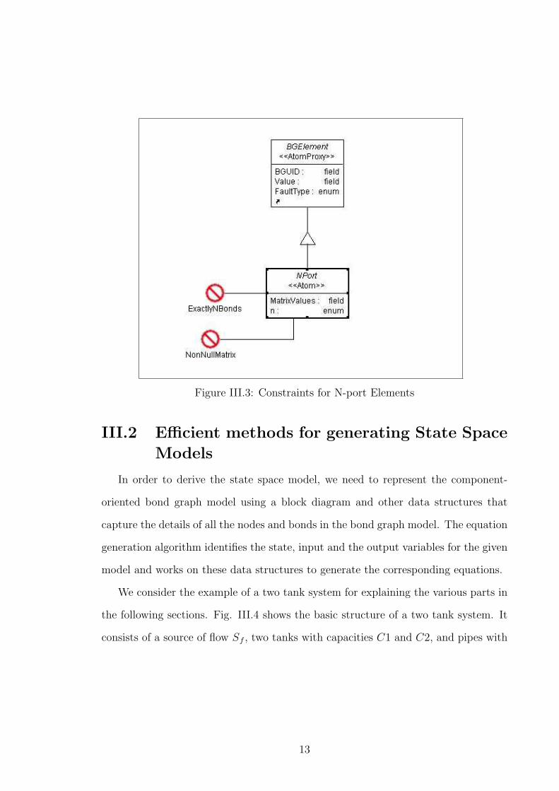
Figure III.3: Constraints for N-port Elements
III.2 Efficient methods for generating State Space
Models
In order to derive the state space model, we need to represent the component-
oriented bond graph model using a block diagram and other data structures that
capture the details of all the nodes and bonds in the bond graph model. The equation
generation algorithm identifies the state, input and the output variables for the given
model and works on these data structures to generate the corresponding equations.
We consider the example of a two tank system for explaining the various parts in
the following sections. Fig. III.4 shows the basic structure of a two tank system. It
consists of a source of flow Sf , two tanks with capacities C1 and C2, and pipes with
13

Figure III.4: Schematic Diagram of a Two Tank System
resistances R1, R2 and R12. Our goal is to measure the outflow rate from tanks 1
and 2 through pipes R1 and R2, respectively.
III.2.1 Data Structures
The basic data structures involved in the Equation Generation algorithm are the
Block Diagram representation of a BG model, a mapping of bond numbers to the
actual bond connections in the BG model, a mapping of junctions in the BG to their
determining bonds and a flat data structure containing the information about all the
nodes in a BG and the connections between them.
Block Diagram Representation
The block diagram (BD) formalism is a widely used graphical, computational
scheme for describing simulation models of continuous and hybrid systems [7].
Fig. III.5 and Fig. III.6 show the causality assignment and the block diagram
structure for every type of element in a bond graph [2]. The Sf, Se, C, and I elements
have a single unique block diagram representation because their incident bonds have
only one possible causal assignment, assuming integral causality for the C and the I
elements. The R, TF and GY elements allow two causal representations each, and
each one produces a different BD representation. A junction with m incident bonds
14

Figure III.5: Fixed and Multi-port Variable Causality Assignments and BD represen-tation
can have m possible BD configurations. Mapping a junction structure to its BD is
facilitated by the notion of the determining bond, which captures the causal structure
for the junction.
Fig.III.7 shows the bond graph model of the two tank system and Fig. III.8 shows
its corresponding block diagram model.
In the BD model of the two tank system, there is a block corresponding to every
node of the BG model and there are Output blocks corresponding to every output
port in the BG model. The Flow1 and Flow2 outputs represent the volume flow rates
measured at pipes R1 and R2, respectively.
Bond Graph Class - A Flat Data Structure
The input for the Equation Generation system is a GME Model constructed using
the extended FACT paradigm. This model represents a simple or a hierarchical bond
graph. To operate on this model, we first need to convert it to a flat model and then
represent the flat model using an appropriate local data structure like an object so
that it can be accessed by various parts of the algorithm without the overhead of
15

Figure III.6: 1- and 2-port Variable Causality Assignments and BD representation
Figure III.7: A GME Bond Graph Model of a Two Tank System
16

Figure III.8: A Block Diagram Model of a Two Tank System
opening or closing text files or the model files. This ensures fast access time making
the algorithm more efficient.
The class BondGraph stores the various details about a given Bond Graph Model
including the specifications for all the nodes in the bond graphs and the connections
that exist between them.
The BondGraph class stores certain properties that are applicable to the entire
bond graph. They can be enumerated as follows:
1. Total number of nodes in the bond graph
2. Total number of junctions in the bond graph
3. Total number of hybrid junctions in the bond graph
4. List of fixed junctions
17

Figure III.9: Template of the Node Data Structure
5. List of determining bonds
6. Sample time
Fig. III.9 shows the data that is stored for every node in the bond graph.
The various data fields can be explained as below:
1. Node identifier
2. Name of the node
3. Type of the node
4. Number of bonds that it is connected to
5. Whether or not it is a potential fault candidate
6. The listing of bonds connected to this node
7. State of the node(On/Off - This parameter is applicable only when the node
under consideration is a hybrid junction. In case of a junction in a continuous
system, this parameter will default to an ”on” value)
8. Whether or not the node (junction) is hybrid
18

9. Index of the node (junction) in the bond graph
10. The parameter n for an n-port element
11. A list of bonds that cannot act as the determining bond for this node (junction).
The bond graph stores the above data for every node in the form of a vector or an
array of the size of the number of nodes in the flat bond graph model. Some of the
properties stated above are populated while generating the data structure from the
Bond Graph GME model, whereas certain others can only be filled in during the later
parts of the algorithm. For instance, since this data structure has been specifically
designed for its use in generating the causality assignment for the bond graph, some
of its properties like the determining bonds list, etc. can only be populated during
the process of running the causality update algorithm.
For storing the connectivity information for the bond graph, that is to capture
the connections between different nodes, each node in the above data structure stores
a set of nodes that it connects to. Thus, the size of this set will be equal to the
number of bonds associated with this node. The order in which the various nodes
appear in this list does not matter as long as we are not dealing with n-port elements.
However, for n-port elements nR, nC and nI, the order is important because the user
associates a distinct number between 1 to n with every bond connected to an n-port
element, and thus the connecting nodes should be listed in the same order as specified
by the user. This helps to associate the index of the connecting node in the list to
the appropriate row in the n × n matrix supplied by the user, in the later parts of
the algorithm.
The node data structure generated for the two tank system is as follows:
Node 1 - TwoTankSystem/TTS/R1
bg.node(1).name = ’//TwoTankSystem/TTS/R1’;
bg.node(1).type = ’R’;
19

bg.node(1).numBonds = 1;
bg.node(1).fault = 0;
bg.node(1).bond(1)= 8;
Node 2 - //TwoTankSystem/TTS/R2
bg.node(2).name = ’//TwoTankSystem/TTS/R2’;
bg.node(2).type = ’R’;
bg.node(2).numBonds = 1;
bg.node(2).fault = 0;
bg.node(2).bond(1) = 9;
Node 3 - //TwoTankSystem/TTS/R12
bg.node(3).name = ’//TwoTankSystem/TTS/R12’;
bg.node(3).type = ’R’;
bg.node(3).numBonds = 1;
bg.node(3).fault = 0;
bg.node(3).bond(1) = 7;
Node 4 - //TwoTankSystem/TTS/C1
bg.node(4).name = ’//TwoTankSystem/TTS/C1’;
bg.node(4).type = ’C’;
bg.node(4).numBonds = 1;
bg.node(4).fault = 0;
bg.node(4).bond(1) = 10;
20

Node 5 - //TwoTankSystem/TTS/C2
bg.node(5).name = ’//TwoTankSystem/TTS/C2’;
bg.node(5).type = ’C’;
bg.node(5).numBonds = 1;
bg.node(5).fault = 0;
bg.node(5).bond(1) = 11;
Node 6 - //TwoTankSystem/TTS/Sf
bg.node(6).name = ’//TwoTankSystem/TTS/Sf’;
bg.node(6).type = ’Sf’;
bg.node(6).numBonds = 1;
bg.node(6).fault = 0;
bg.node(6).bond(1) = 10;
Node 7 - //TwoTankSystem/TTS/OJ
bg.node(7).name = ’//TwoTankSystem/TTS/OJ’;
bg.node(7).type = ’OneJunction’;
bg.node(7).numBonds = 3;
bg.node(7).state = 1;
bg.node(7).index = 1;
bg.node(7).hybrid = 0;
bg.node(7).bond(1) = 10;
bg.node(7).bond(2) = 11;
bg.node(7).bond(3) = 3;
21

Node 8 - //TwoTankSystem/TTS/OJ1
bg.node(8).name = ’//TwoTankSystem/TTS/OJ1’;
bg.node(8).type = ’OneJunction’;
bg.node(8).numBonds = 2;
bg.node(8).state = 1;
bg.node(8).index = 2;
bg.node(8).hybrid = 0;
bg.node(8).bond(1) = 10;
bg.node(8).bond(2) = 1;
Node 9 - //TwoTankSystem/TTS/OJ2
bg.node(9).name = ’//TwoTankSystem/TTS/OJ2’;
bg.node(9).type = ’OneJunction’;
bg.node(9).numBonds = 2;
bg.node(9).state = 1;
bg.node(9).index = 3;
bg.node(9).hybrid = 0;
bg.node(9).bond(1) = 11;
bg.node(9).bond(2) = 2;
Node 10 - //TwoTankSystem/TTS/ZJ1
bg.node(10).name = ’//TwoTankSystem/TTS/ZJ1’;
bg.node(10).type = ’ZeroJunction’;
bg.node(10).numBonds = 4;
bg.node(10).state = 1;
bg.node(10).index = 4;
22

bg.node(10).hybrid = 0;
bg.node(10).bond(1) = 6;
bg.node(10).bond(2) = 7;
bg.node(10).bond(3) = 4;
bg.node(10).bond(4) = 8;
Node 11 - //TwoTankSystem/TTS/ZJ2
bg.node(11).name = ’//TwoTankSystem/TTS/ZJ2’;
bg.node(11).type = ’ZeroJunction’;
bg.node(11).numBonds = 3;
bg.node(11).state = 1;
bg.node(11).index = 5;
bg.node(11).hybrid = 0;
bg.node(11).bond(1) = 7;
bg.node(11).bond(2) = 5;
bg.node(11).bond(3) = 9;
bg.numNodes = 11;
bg.numJunctions = 5;
bg.numHybridJunctions = 0;
Causality Assignment
Bond Graph models imply a causal structure and algorithms like the Sequential
Causality Assignment Procedure (SCAP) [8] applied to well-formed BG models assign
causal directions to all bonds in the model.
23

Figure III.10: Algorithm for assigning Bond numbers
After executing SCAP, every junction in the BG model is assigned a determining
bond; this data is further used in the equation generation algorithm. The determining
bond assignment for the two tank system model can be given as:
JunctionName ---> DeterminingBond
TwoTankSystem/TTS/OJ ---> TwoTankSystem/TTS/R12
TwoTankSystem/TTS/OJ1 ---> TwoTankSystem/TTS/R1
TwoTankSystem/TTS/OJ2 ---> TwoTankSystem/TTS/R2
TwoTankSystem/TTS/ZJ1 ---> TwoTankSystem/TTS/C1
TwoTankSystem/TTS/ZJ2 ---> TwoTankSystem/TTS/C2
Assigning Bond Numbers
The equations that are generated have effort and flow variables associated with
different bonds. In order to generate these equations, we need to assign numbers to all
the bonds in the bond graph model. The algorithm for assigning the bond numbers
shown in Fig. III.10 operates on the the list of nodes that is a part of the BondGraph
class described above.
The algorithm AssignBondNumbers iterates over all the nodes in the bond graph.
24

For every node, it iterates over all the connecting nodes associated with that particular
node. If that pair of nodes has already been assigned a bond number (the order of
nodes in the pair is immaterial), then it skips over to the next node, else it adds it to
the bonds data structure; the index of the pair in the data structure automatically
becomes the bond number associated with that pair.
Following is the bond number assignment made by the algorithm for the given
two tank BG model.
Bond 1: R1 - OJ1
Bond 2: R2 - OJ2
Bond 3: R12 - OJ
Bond 4: C1 - ZJ1
Bond 5: C2 - ZJ2
Bond 6: Sf - ZJ1
Bond 7: OJ - ZJ1
Bond 8: OJ - ZJ2
Bond 9: OJ1 - ZJ1
Bond 10:OJ2 - ZJ2
Storing variable coefficients
For a given input model, we need to extract the sets of input, state and output
variables. Input variables are associated with the flows and efforts associated with
Sf and Se blocks respectively. State variables are the efforts on the capacitances and
the flows through the inertias. The flow through a one-junction or an effort at a
zero-junction to which a sensor has been connected, form the output variables.
Thus, for the two tank system, we observe that f6, i.e., the flow associated with
25

Sf is the input variable, e4 and e5, i.e., the efforts on the two capacitances are the
state variables, and f1 and f2, i.e., the flows measured at the two one junctions are
the output variables.
Each equation that is generated is represented in terms of the state and the input
variables. Thus, for every variable for which we need to generate an equation we
need to associate it with a map; the key of this map is the state or the input variable
index and the value is the coefficient associated with that variable for that particular
equation. Initially, for each state or input variable in the map, the coefficient value is
equal to zero. The value part keeps on getting updated during the equation generation
process. When the equation generation algorithm has been executed for a given
variable, we finally get a map which will have non-zero coefficient values for all the
state and input variable taking part in the equation. If we need to generate the
equations in symbolic form, this coefficient value is represented as a string instead of
representing it in a numeric form.
III.2.2 State Equation Generation Algorithm
The GenerateStateEquations algorithm is used to generate the state equations
given a Block Diagram bd. This block diagram is a computational representation
of the given bond graph; it has blocks corresponding to every element in the bond
graph. It also captures the connections between the different blocks in the form of
input and output signals.
As seen in the previous section, for a given physical system represented by a bond
graph, we have the flows through the inertias and the efforts on the capacitances as
the state variables. The basic EquationGeneration algorithm described in Fig. III.13
is called for each of these state variables. The goal of the basic equation generation
26

algorithm is to represent a given flow or an effort variable associated with a particular
bond in terms of state variables and input variables of the system.
For a capacitive element, with an associated effort e, flow f, and capacitance C,
we have the state variable e represented as
e =1
C· f
Similarly, for an inductive element, with an associated effort e, flow f, and induc-
tance I, we have the state variable f represented as
f =1
I· e
The basic principle in generating equations from a block diagram is to backtrack
from the block under consideration till a point where we end up with a set of effort
or flow signals associated with blocks that either represent the input variables of the
system or the state variables.
We illustrate the working of this algorithm by stepping through the equation gen-
eration process for one of the state variables of the two tank system. Fig. III.11
shows the execution trace for the equation generation algorithm for e5. The pa-
rameters passed to the GenerateFurther function i.e., the Basic Equation Generation
algorithm, are the coefficient, the bond variable (The variable is typically represented
as a 〈 flow, bond number 〉 variable or an 〈 effort, bond number 〉 variable) and the
name of the source block. We keep on backtracking till we reach a state variable or
an input variable at which point we prune that branch of the tree. As we can see in
Fig. III.11, the branches get pruned when we reach the state variables e4 and e5.
The state equation generation algorithm is as shown in Fig. III.12.
By running this algorithm, we are able to obtain the representation of every state
27
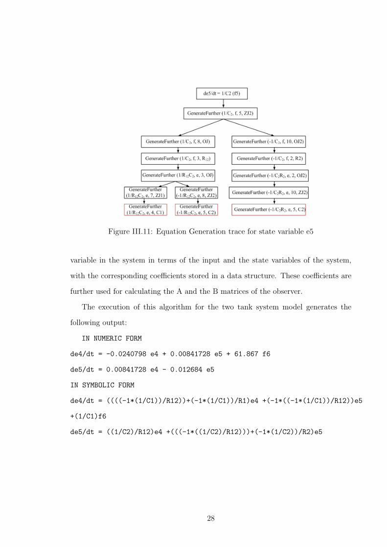
Figure III.11: Equation Generation trace for state variable e5
variable in the system in terms of the input and the state variables of the system,
with the corresponding coefficients stored in a data structure. These coefficients are
further used for calculating the A and the B matrices of the observer.
The execution of this algorithm for the two tank system model generates the
following output:
IN NUMERIC FORM
de4/dt = -0.0240798 e4 + 0.00841728 e5 + 61.867 f6
de5/dt = 0.00841728 e4 - 0.012684 e5
IN SYMBOLIC FORM
de4/dt = ((((-1*(1/C1))/R12))+(-1*(1/C1))/R1)e4 +(-1*((-1*(1/C1))/R12))e5
+(1/C1)f6
de5/dt = ((1/C2)/R12)e4 +(((-1*((1/C2)/R12)))+(-1*(1/C2))/R2)e5
28
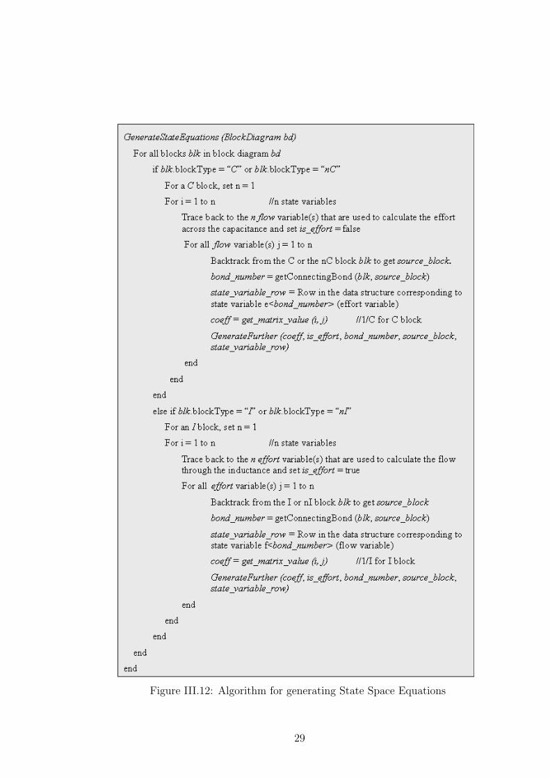
Figure III.12: Algorithm for generating State Space Equations
29

III.2.3 Output Equation Generation Algorithm
The output equation generation algorithm invokes the basic equation generation
algorithm for the output variables in exactly the same way as the state equation
generation algorithm that invoked the basic equation generation algorithm for the
state variables. In order to identify the output variable, we scan the Block Diagram
for Output blocks and then trace back from them till we reach a block representing
either a One Junction or a Zero Junction. A sensor connected to a one junction
implies that the flow at that junction is measured, whereas a sensor connected to a
zero junction implies that the effort at that junction is to be measured. To measure
the flow or effort at a one or a zero junction respectively, we consider the determining
bond for the junction, and then invoke the basic equation generation algorithm for
these parameters.
For the two tank system model, f1 and f2 are the output variables. The equations
generated for these variables are given as:
IN NUMERIC FORM
f1 = 0.000253165 e4
f2 = 6.89655e-005 e5
IN SYMBOLIC FORM
f1 =((1)/R1)e4
f2 = ((1)/R2)e5
III.2.4 Basic Equation Generation Algorithm
The basic equation generation algorithm encapsulates the basic step of backtrack-
ing required to generate an equation for any variable. This algorithm will be called
multiple times for generating an equation for a given state or an output variable. It
30

takes as its input, a source block blk in a Block Diagram that has been derived from
a bond graph, the variable v for which we are interested in generating an equation for
in the form of 〈is effort, bond number 〉 (the Boolean value is effort indicates whether
we are determining an effort or a flow, and the bond number indicates the bond corre-
sponding to the variable), the coefficient which is the multiplier of this variable in the
entire equation of which the variable is a part, and the row id.( The variable under
consideration is a part of the equation that is being generated for another variable w.
So, the row id gives the row corresponding to the variable w.)
The algorithm is as shown in Fig. III.13
The equation generation procedure aims at expressing any given variable in terms
of state variables and input variables. So, the algorithms checks for this condition in
the very beginning. It terminates when it finds that v is either a state variable or an
input variable, by storing the value of the coefficient for v. If the variable v is not
a state or an input variable, the behavior of the algorithm varies depending on the
type of block blk.
The working of the algorithm for the equation generation of a state variable in
the two tank system can be seen in Fig. III.11.
III.2.5 Extension for Transformers and Gyrators
The following condition checks are added to the basic equation generation algo-
rithm so that it can handle bond graphs having transformer and gyrator elements.
If the block type corresponds to a Transformer block TF, we get the node number
corresponding to the bond number that was passed as an argument. Also, get the
transformer ratio value n. Then we find out if the bond that is passed is an input to
the TF or an output, and also find its corresponding input or output index. We also
find the node corresponding to the other bond of the transformer as we need that to
31

32

33

Figure III.13: Basic Equation Generation Algorithm
Figure III.14: Causal assignments and corresponding equations for a Transformer
continue the equation generation. For a transformer, we have the following two cases
as shown in Fig. III.14.
From the given equations we see that, if the variable that we are considering for
equation generation var is e1, then we need to call the basic equation generation
algorithm for e2 with the coefficient value multiplied by n. If the variable var is e2,
then we need to call the basic equation generation algorithm for e1 with the coefficient
value divided by n. Similarly, if var is f1, then we need to call the basic equation
generation algorithm for f2 with the coefficient value divided by n and if var is f2,
then we need to call the basic equation generation algorithm for f1 with the coefficient
value multiplied by n.
Now, if the block type corresponds to a Gyrator block GY, we get the node number
corresponding to the bond number that was passed as an argument. Also, get the
34

Figure III.15: Causal assignments and corresponding equations for a Gyrator
gyrator ratio value r. Then we find out if the bond that is passed is an input to the
GY or an output, and also find its corresponding input or output index. We also
find the node corresponding to the other bond of the transformer as we need that to
continue the equation generation. For a gyrator, we have the following two cases as
shown in Fig. III.15.
From the given equations we see that, if the variable that we are considering for
equation generation var is e1, then we need to call the basic equation generation
algorithm for f2 with the coefficient value multiplied by r. If the variable var is e2,
then we need to call the basic equation generation algorithm for f1 with the coefficient
value multiplied by r. Similarly, if var is f1, then we need to call the basic equation
generation algorithm for e2 with the coefficient value divided by r and if var is f2,
then we need to call the basic equation generation algorithm for e1 with the coefficient
value divided by r.
III.2.6 Extensions to SCAP
In order to assign causalities to a BG model containing n-port elements, it is
necessary to extend SCAP [8] to assign appropriate causalities to the bonds connected
to the n-port elements. The n-port capacitance nC and the n-port inductance nI have
a preferred integral causality, thus nC determining the effort on all n incident bonds
35

Figure III.16: Causality Assignment for nC and nI
and nI determining the flow for all n incident bonds. Fig. III.16 shows nC and nI in
preferred integral causalities.
The n-port resistance nR exhibits indifferent causality just like its single port
counterpart. The next chapter explains the handling of n-port elements in greater
detail with the help of a sample system.
III.3 Building the Kalman Filter
The Kalman filter provides a mechanism for estimating the state of a discrete-time
controlled process that is governed by a set of linear stochastic difference equations.
After identifying the state and the output variables of the system and after gener-
ating the corresponding equations for them using the state and the output equation
generation algorithms, we obtain the matrices A, B, C and D such that they satisfy
the following equations:
˙X(t) = FX(t) + GU(t)
Y (t) = CX(t) + DU(t)
The second equation is in the form expected by the Kalman filter. However, we
36

need to transform the first equation from continuous to discrete form to get it in the
following form:
X(t) = AX(t− 1) + BU(t− 1)
To convert from the continuous to discrete form, the method previously used [6]
was the Zero Order Hold Discretization method. However, this is a crude approximate
discretization and may not suffice to represent the dynamics of complex systems in
a sufficiently accurate manner. First Order Hold, and Impulse trains are some of the
other methods that can be used for the purpose of discretization. These methods are
implemented by the c2d function in MATLAB [13] and will be used in the future to
get more accurate results.
The values of the measurement noise covariance R, the process noise covariance
Q, and the initial values for the set of state variables X, the initial values for the set
of input variables U and the initial values for the estimation error covariance P are
user-defined. Similarly, the period for which the simulation is run and the sampling
frequency are all user-defined.
Fig. III.17 [4] shows the complete operation of the Kalman filter, including all the
equations. Based on the values of the matrices A, B, C, D (after converting F, G to
discrete time A, B) and the user inputs, the time update or the predictor equations [4]
are executed for projecting forward (in time) the current state and error covariance
estimates for the next time step.
These are followed by the execution of the measurement update or the correc-
tor equations [4] that are responsible for the feedback i.e. for incorporating a new
measurement into the a priori estimate to obtain an improved a posteriori estimate.
This process is continued for period equal to the one entered by the user at the given
sampling frequency.
37

Figure III.17: Kalman Filter Equations for Process and Measurement Model
For the two tank system example that we have considered, the values for matrices
A, B, C and D generated by our implementation are as follows:
The values of matrices A, B, C and D are given as:
A matrix:
[0.999759 8.41728e-005 ; 8.41728e-005 0.999873]
B matrix:
[0.61867 0]
C matrix:
[0 6.89655e-005; 0.000253165 0]
D matrix:
[0 0]
The Kalman filter is built based on the above matrices and it takes the outputs
from the Simulink model to produce a set of estimated output values. The set of
estimated output values and the system generated output values for f1 and f2 are
plotted against time in Fig. III.18
38

Figure III.18: Observer and System Output for a Two Tank System
39

By looking at the plot, it can be observed that our implementation of the observer
closely tracks the system output. It does so in the presence of noise as well.
40

CHAPTER IV
EXPERIMENTAL RESULTS
In order to test our system for generating the state space and the output equations
and the building of the Kalman filter, we consider two different systems.
IV.1 Hydraulic Actuator System
A simplified model of a hydraulic actuator system is shown in Fig. IV.1 [11].
Figure IV.1: A simplified model for the Hydraulic Actuator
The actuator is composed of a single chamber, piston of cross sectional area A
and volume of the chamber Vo. The pressure difference between the right and the
left sides of the chamber produces the force for piston displacement. The piston is
connected to the load which is modeled as a simple mass spring damper system.
A centrifugal pump system is defined in terms of its input voltage and current,
internal variables such as torque and angular velocity and output variables, such as
fluid pressure and fluid flow rate. The energy transmitted to the pump is expended
in turning the veins of the pump rotor. In the process, the fluid is pushed out with
a certain pressure and flow rate. This flow of the liquid helps in moving the piston
cylinder of the actuator system back and forth which in turn is connected to the load.
41

Table IV.1: Description of the Actuator Parameters
Parameter DescriptionA Cross sectional area of the pistonV0 Volume of the chamberβ Bulk density of the fluidRv Resistance of the valveSe Effort sourcepr Chamber’s pressure at right sidepl Chamber’s pressure at left side
pr − pl Pressure differenceM Massk Spring stiffnessB Damping coefficient
u(t) Displacement of the mass
IV.1.1 Equation Generation for the Hydraulic Actuator Sys-tem
Fig.IV.2 shows the bond graph model of the actuator system described above.
When this BG model is fed as an input to our implementation of the Equation
Generation Algorithm, the following state equations are generated for state variables
f5, e6, e7 and e8.
Figure IV.2: A GME Bond Graph Model of Hydraulic Actuator System
42

IN SYMBOLIC FORM
df5/dt = (-1*B friction)*(1/Mass) f5 - ((1/Mass)*TF2)e6 - (1/Mass)e7 + ((1/Mass)*TF)
e8
de6/dt = ((1/C2)*TF2) f5 - ((1/C2)/R pipe) e6 + ((1/C2)/R pipe) e10
de7/dt = (1/C spring) f5
de8/dt = (-1*(1/C1)*TF2) f5 + (-1*((1/C1)/R valve)) e8 + (((1/C1)/R valve)*TF1)
e9
In the above equations, f5 is the flow associated with the inertia Mass, e6 is
the effort associated with the capacitance C2, e7 is the effort associated with the
capacitance C spring, and e8 is the effort associated with the capacitance C1. Effort
e9 associated with the source of effort Se and the effort e10 associated with the source
of effort Se cap are the input variables of the system.
The following output equations are generated for the system:
f5 = f5
e6 = e6
e8 = e8
f13 = (TF2) f5,
where f5 is the Velocity sensor, e6 is the Cap 2 sensor, e8 is the Cap 1 sensor and f13
senses the pressure difference.
The Simulink model for this system and one of the outputs (pressure output) is
shown in Fig. IV.3 and IV.4, respectively.
IV.1.2 Observer runs with measurement noise and modelingerrors in the system model
For the purpose of analyzing the behavior of the observer under the presence of
noise in the measurement and/or modeling errors, we consider a part of the actuator
system described in the previous subsection. The current implementation of our
43

Figure IV.3: Simulink Model of the Hydraulic Actuator System
0 5 10 15 20 25 30 35 40 45 50-1
-0.5
0
0.5
1
1.5
2
2.5
3
3.5
4x 10
-5
Time offset: 0
Figure IV.4: Pressure Output of the Hydraulic Actuator System
44

Figure IV.5: A GME Bond Graph Model of a part of the Hydraulic Actuator System
observer only supports linear systems; hence, we restrict ourselves to a part of the
hydraulic actuator.
Fig. IV.5 shows the bond graph model of the part of the actuator system under
consideration. The different components in the bond graph model are explained as
below:
R is the resistance of the pipe connected from the pump to the cylinder of the
actuator. Se represents the effort output of the centrifugal pump that drives the
actuator. The transformer TF1 models the conversion of mechanical energy to fluid
energy. The resistive element R valve is used to control the flow of the liquid through
the pipes. The capacitance C1 models the variable volume of the right hand side of
the cylinder.
From the bond graph model, we observe that the system contains one state vari-
able, i.e. the effort associated with the capacitance C1, one input variable i.e. the
effort imposed by Se, and two measured variables - flow through R valve and effort
across the capacitance C1.
45

Our system generates the following causality assignment for the given bond graph:
JunctionName ---> DeterminingBond
Component/1J1 ---> Component/R valve
Component/0J ---> Component/C1
Component/TF Bug ---> Component/TF1
Component/0J1 ---> Component/Se
The bond numbers are assigned as follows: Bond 1: R valve - 1J1
Bond 2: R - 0J1
Bond 3: R Cap - 0J
Bond 4: C1 - 0J
Bond 5: Se - 0J1
Bond 6: TF1 - 0J1
Bond 7: TF1 - TF Bug
Bond 8: 1J1 - TF Bug
Bond 9: 1J1 - 0J
The following equations are generated by our system.
State space equations:IN NUMERIC FORM
de4/dt = -0.1001e4+0.0001e5
IN SYMBOLIC FORM
de4/dt = (((-1*((1/C1)/R valve))) +(-1*(1/C1))/ R Cap) e4 +(((1/C1)/ R valve)/
TF1) e5
Output equations:
IN NUMERIC FORM
46
f1 = -1e-005 e4 + 1e-005 e5
e4 = 1e4
IN SYMBOLIC FORM
f1 = (-1*((1)/ R valve)) e4 + (((1)/R valve)/ TF1) e5
e4 = (1)e4
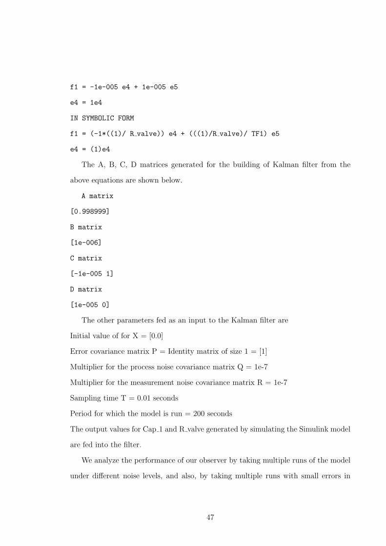
The A, B, C, D matrices generated for the building of Kalman filter from the
above equations are shown below.
A matrix
[0.998999]
B matrix
[1e-006]
C matrix
[-1e-005 1]
D matrix
[1e-005 0]
The other parameters fed as an input to the Kalman filter are
Initial value of for X = [0.0]
Error covariance matrix P = Identity matrix of size 1 = [1]
Multiplier for the process noise covariance matrix Q = 1e-7
Multiplier for the measurement noise covariance matrix R = 1e-7
Sampling time T = 0.01 seconds
Period for which the model is run = 200 seconds
The output values for Cap 1 and R valve generated by simulating the Simulink model
are fed into the filter.
We analyze the performance of our observer by taking multiple runs of the model
under different noise levels, and also, by taking multiple runs with small errors in
47

Figure IV.6: Measured and Observed values for Actuator for a measurement noise of2 percent
model parameters along with some noise. Also, for each run, we calculate the mean
squared value of the error in order to verify the working of the observer.
Figures IV.6, IV.7, IV.8 plot the measured and the observed outputs for noise
values of 2, 5 and 8 percent in the measurement respectively. From Table IV.2, we
can see that the mean square error increases as the measurement noise increases.
Next, we run the observer for a measurement noise of 2 percent and by introducing
errors of 2, 5 and 8 percent in the parameter values of the input torque Se and the
valve resistance Rvalve simultaneously. When the torque is increased and the resistance
decreased, the volume displaced increases whereas, when the torque is decreased and
the valve resistance increased, we observe that the volume displaced decreases. This
48
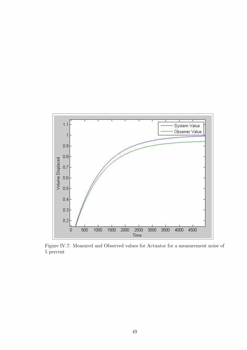
Figure IV.7: Measured and Observed values for Actuator for a measurement noise of5 percent
49
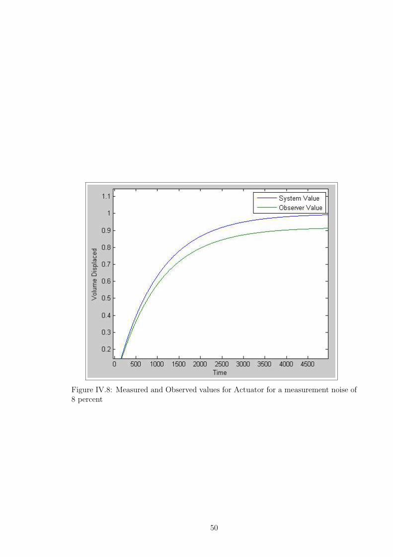
Figure IV.8: Measured and Observed values for Actuator for a measurement noise of8 percent
50

Figure IV.9: Measured and Observed values for Actuator for a measurement noise of2 percent, Se increased by 2 percent and R valve decreased by 2 percent
concurs with the expected behavior of the system. Figures IV.9, IV.10 and IV.11
show the plots for the same.
Table IV.2: Mean Square Error Values
Noise % Error % in Se Error % in Rvalve Mean squared error Error %2 0 0 1.09712e-7 1.622e-75 0 0 1.27299e-7 1.953e-78 0 0 1.48611e-7 2.017e-72 +2 -2 1.18849e-7 1.455e-72 -5 +5 9.01745e-8 1.27e-72 +8 -8 1.51785e-7 1.647e-7
51
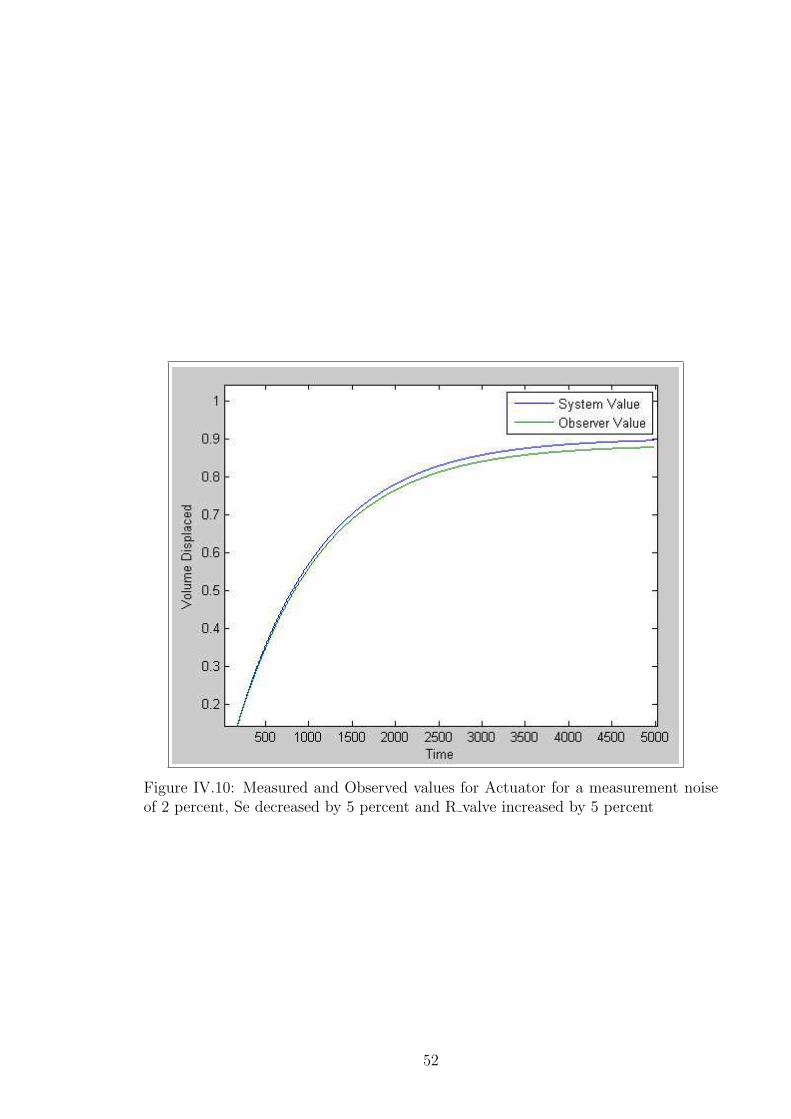
Figure IV.10: Measured and Observed values for Actuator for a measurement noiseof 2 percent, Se decreased by 5 percent and R valve increased by 5 percent
52

Figure IV.11: Measured and Observed values for Actuator for a measurement noiseof 8 percent, Se increased by 2 percent and R valve decreased by 8 percent
53
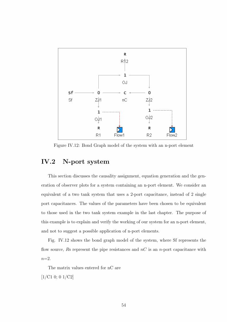
Figure IV.12: Bond Graph model of the system with an n-port element
IV.2 N-port system
This section discusses the causality assignment, equation generation and the gen-
eration of observer plots for a system containing an n-port element. We consider an
equivalent of a two tank system that uses a 2-port capacitance, instead of 2 single
port capacitances. The values of the parameters have been chosen to be equivalent
to those used in the two tank system example in the last chapter. The purpose of
this example is to explain and verify the working of our system for an n-port element,
and not to suggest a possible application of n-port elements.
Fig. IV.12 shows the bond graph model of the system, where Sf represents the
flow source, Rs represent the pipe resistances and nC is an n-port capacitance with
n=2.
The matrix values entered for nC are
[1/C1 0; 0 1/C2]
54

where C1 and C2 correspond to the values of the two capacitances used in the equiv-
alent system with 2 one-port capacities. By making use of the extended version
of SCAP that supports n-port elements, the causalities get assigned in such a way
that nC determines the effort at both the zero junctions connected to it. The bond
assignment for the system is as shown below:
Bond 1: R1 - OJ1
Bond 2: R2 - OJ2
Bond 3: R12 - OJ
Bond 4: nC - ZJ1
Bond 5: nC - ZJ2
Bond 6: Sf - ZJ1
Bond 7: OJ - ZJ1
Bond 8: OJ - ZJ2
Bond 9: OJ1 - ZJ1
Bond 10:OJ2 - ZJ2
The flow associated with Sf is the input variable f6. The efforts e4 and e5
associated with nC are the two state variables in the system and the volume flow
rates measured at the two one junctions, namely f1 and f2 are the output variables
of the system.
The state equations generated for the system are:
IN NUMERIC FORM
de4/dt = -0.0240798 e4 + 0.00841728 e5 + 61.867 f6
de5/dt = 0.00841728 e4 - 0.012684 e5
IN SYMBOLIC FORM
de4/dt = ((((-1*(1/nC(1,1)))/R12))+(-1*(1/nC(1,1)))/R1)e4 +(-1*((-1*(1/nC(1,1)))/R12))e5
55

+(1/nC(1,1))f6
de5/dt = ((1/nC(2,2))/R12)e4 +(((-1*((1/nC(2,2))/R12)))+(-1*(1/nC(2,2)))/R2)e5
The output equations generated for the system are:
IN NUMERIC FORM
f1 = 0.000253165 e4
f2 = 6.89655e-005 e5
IN SYMBOLIC FORM
f1 =((1)/R1)e4
f2 = ((1)/R2)e5
The values of the Kalman filter matrices A, B, C, D are: The values of matrices
A, B, C and D are given as:
A matrix:
[0.999759 8.41728e-005 ; 8.41728e-005 0.999873]
B matrix:
[0.61867 0]
C matrix:
[0 6.89655e-005; 0.000253165 0]
D matrix:
[0 0]
We see that these values correspond to those generated for the equivalent two
tank system model considered in the previous chapter, and are thus able to verify the
working of our implementation for an n-port system.
The plot of the measured and the observed volume flow rate outputs against time
is as shown in Fig. IV.13.
56

Figure IV.13: Observer and System Output for a Two Tank System implementedusing nC
57

From the above two examples the correctness of our implementation can be veri-
fied.
58
CHAPTER V
CONCLUSIONS
After testing the implementation of our system for different component-based
bond graph models of linear systems, we have verified the working of the our equation
generation algorithm and our Kalman filter implementation. Also, by running the
observer for multiple sets of data containing measurement noise and modeling errors,
we observed, as expected, that the mean squared error increased with the increase
in the measurement noise or with the increase in the deviation of model parameters
from their nominal values, however, the observer still managed to track the system
dynamics within acceptable error bounds.
V.1 Future Work
The current system works for models of linear systems. However, most com-
plex systems contain a number of non linearities, and an important extension to the
current algorithm will be to support such non-linearities by extending the equation
generation algorithm to handle modulated elements and function blocks and changing
the implementation of the observer from the Kalman filter to the Extended Kalman
Filter. This will also allow us to build bond graph models containing n-port elements
where the transfer matrix coefficients will not have to be constant values.
Another extension to our present implementation would be to support hybrid
systems which are modeled as Hybrid Bond Graphs. The causality assignment and
the equation generation algorithm will have to take the junction state into account,
and make the effective changes to the system model.
59

BIBLIOGRAPHY
[1] T. Wong, P. Bigras, K. Khayati, “Causality assignment using multi-objective evo-lutionary algorithms”, Systems, Man and Cybernetics, 2002 IEEE InternationalConference on Volume 4, 6-9 Oct. 2002, On page(s): 6 pp.
[2] I. Roychoudhury, M. Daigle, G. Biswas, X. Koutsoukos, P. J. Mosterman, “AMethod for Efficient Simulation of Hybrid Bond Graphs”, International Confer-ence on Bond Graph Modeling and Simulation (ICBGM 2007) January, 2007, pp.177-184
[3] - J. Broenink, “Bond-Graph Modeling in Modelica”, European Simulation Sym-posium 1997 Oct. 19-22
[4] G. Welch, G. Bishop, “An Introduction to the Kalman Filter”, Department ofComputer Science, University of North Carolina at Chapel Hill
[5] G. Karsai, G. Biswas, S. Abdelwahed, N. Mahadevan, E. Manders, “Model-basedsoftware tools for integrated vehicle health management”, Space Mission Chal-lenges for Information Technology, 2006. SMC-IT 2006. Second IEEE Interna-tional Conference on 17-20 July 2006, On page(s): 8 pp.
[6] FACT Documentation
[7] M. Daigle, I. Roychoudhury, G. Biswas, X. Koutsoukos, “Efficient Simulation ofComponent-Based Hybrid Models Represented as Hybrid Bond Graphs”, Tech-nical Report ISIS-06-712, Institute for Software Integrated Systems, VanderbiltUniversity Dec 2006
[8] D. Karnopp, D. Margolis, R. Rosenberg, “Systems Dynamics: Modeling and Sim-ulation of Mechatronic Systems”, Third edn. John Wiley Sons, Inc., New York2000
[9] J. Broenink, “Introduction to Physical Systems Modeling with Bond Graphs”,University of Twente, Dept EE, Control Laboratory
[10] P. Mosterman, G. Biswas, “Diagnosis of continuous valued systems in transientoperating regions”, Systems, Man and Cybernetics, Part A, IEEE Transactionson, Volume 29, Issue 6, Nov 1999, pp. 554 - 565
[11] A. Moustafa, G. Biswas, S. Mahadevan, “Fault Diagnosis of Hydraulic Actuatorsusing Bond Graphs”, Progress Report for August 2007
[12] E. Manders, P. Mosterman, G. Biswas, L. Barford, “TRANSCEND: A Systemfor Robust Monitoring and Diagnosis of Complex Engineering Systems”, Jan 141999
60

[13] MATLAB Documentation
61