May 2007, Volume 46, No. 5 35

An Effective Method for Modelling Non-Moving Stagnant Liquid Columns

in Gas Gathering Systems

R.G. McNeil, D.R. lillico Fekete Associates inc.

Peer reviewed PaPer (“review and Publication Process” can be found on our web site)

IntroductionThe maturation of the gas gathering systems throughout North

America has resulted in the majority of systems being operated well below their original design conditions. Consequently, it is common to encounter pressure losses that exceed those predicted by steady-state single-phase and two-phase correlations. The rea-sons for these pressure losses are varied and most often relate to measurement issues, poor understanding of the pipeline and fa-cility connections and sometimes non-moving liquid accumula-tions called stagnant liquid columns. Liquid accumulations are a concern because their continuous removal is difficult and they in-crease backpressure for all upstream wells, which reduces well de-liverability and can result in localized pipeline corrosion.

One would think that the traditionally used steady-state two-phase pressure loss equations would be capable of predicting the pressure loss that occurs in these liquid accumulations. However, the steady-state flow of fluid must be, by definition, continuous: inlet rate equal to outflow rate. If the liquid enters the conduit and accumulates while the gas continues through, we no longer have steady-state flow and the validity of the correlation no longer holds.

It has been the authors’ experience that localized pressure losses are often associated with liquid accumulations. Typically, field staff usually know there is a problem and may or may not have al-ready realized that it is due to liquids, but it is usually a surprise for head-office staff because there is little or no liquid production reported.

This leads to the question, how do we reliably identify stagnant liquid columns and how should they be modelled? To answer this question, a discussion of recommended modelling procedures is required.

Abstract Gas gathering system modelling is often complicated by

the presence of localized pressure losses that are not easily ex-plained by traditional pressure loss correlations. The tendency is to assume the pressure loss correlation must be tweaked to match measured operating conditions. This often leads to inappropriate manipulation of tuning factors (efficiency factor or roughness).

A more appropriate approach is to recheck the validity of the input data and, most importantly, visit the field prepared to gather additional data to resolve the causes of the localized pres-sure losses. The objectives of this paper are to discuss one of the causes of localized pressure losses—Stagnant Liquid Columns—and to present several cases where localized pressure losses were interpreted to be caused by stagnant liquid accumulations.

Discussion

Pressure loss categorizationThe existing steady-state pressure loss correlations generally do

a very good job of estimating pressure losses when used appro-priately. Consequently, a comparison of simulated line pressures with field measured line pressures should result in a reasonable match within a preset tolerance. Measured line pressures that do not match modelled line pressures must be scrutinized closely to determine the cause of the mismatch, rather than relying primarily on tweaking tuning factors such as pipeline roughness or flow efficiency.

For wells or groups of wells where a reasonable match is not initially obtained, it is good practice to begin by attempting to clas-sify the unmatched pressure losses as either a systemic or localized step pressure loss problem before making changes to the model to force a match.

Systemic pressure losses manifest as a gradual or cumulative degradation in the match as you look further upstream from the model start point (point where a flowing pressure is a given). Sys-temic pressure loss problems are always due to incorrect pipeline specifications, the presence of too much fluid (gas and liquid), the presence of too little fluid or the specification of an inappropriate pressure loss correlation.

Step pressure losses manifest at a point in the pipeline system where all wells downstream of that point match within the preset tolerance, and all wells upstream of that point exhibit a consistent step increase in pressure over that predicted by the pressure loss correlation. Step pressure losses are usually friction-based if as-sociated with a plant inlet or header, and are usually hydrostatic-based if located in a pipeline between wells.

Since total pressure loss is largely the sum of the friction and hy-drostatic pressure loss, it is also good practice for modellers to get into the habit of classifying every step pressure loss as either fric-tion-dominated flow or hydrostatic-dominated flow. Since hydro-static pressure loss is governed by Equation (1):

∆P ghh = ρ............................................................................................... (1)

we can assume hydrostatic pressure losses can be represented as fixed pressure loss. Obviously, this is an approximation as the den-sity of a two-phase mixture depends upon the proportions of gas and liquid.

For single-phase flow, the Fanning correlation, as shown in Equation (2), governs friction pressure loss:

36 Journal of canadian Petroleum Technology

∆Pf v L

gDf = ρ 2

2........................................................................................ .(2)

Since friction pressure loss is a function of the square of the gas velocity, friction pressure loss increases non-linearly with respect to gas flow rate.

Figure 1 presents an example of the friction pressure loss vs. gas flow rate for a pipeline. Note that changing the pipe roughness has very little impact on pressure loss at low gas rates [less than 14 103m3/d (500 Mscfd)] for this example, but has a dramatic effect on pressure loss for high gas rates. It is obvious that attempting to use the friction-based tuning factors (roughness or efficiency) to tune a low flow rate pipeline is not advisable. A solution can some-times be forced with the overuse of roughness or efficiency, but the result is usually a model that can reproduce only current con-ditions. These models invariably fail when simulating before and after conditions for field modifications that significantly change gas flow rates or operating pressures.

The same argument applies to two-phase flow since all two-phase correlations utilize a modified form of Fanning or an approx-imation of Fanning. The main difference being that the procedure begins with the calculation of liquid holdup that is then used to cal-culate a two-phase friction factor, a two-phase density and a two-phase velocity.

Figure 2 presents one pipeline leg of a gas gathering system. Each well in the leg displays the well name, model calculated line pressure and measured line pressure. Note that working out-ward from the plant, the calculated and measured line pressure for the wells 02-10, 11-02 and 06-01 all match very closely. Also, note the calculated and measured line pressure for the wells 06-27 and 06-36 differ by 855 kPa (124 psi) and 786 kPa (114 psi), respectively.

Since the line pressures for the first three wells (02-10, 11-02 and 06-01) all match closely and the next two wells differ by very similar values, it is deduced that the difference in calculated and measured line pressures at the wells 06-27 and 06-36 is most likely a localized step pressure loss problem. The location of the problem(s) could be at each well site, in the tie-in pipelines or in the common pipeline that ties into the well 11-02 location with its endpoints labeled A and B. It is deduced that the pressure loss most likely occurs in the link between points A and B, since this is the simpler solution.

Although the problem identified could be a partially closed valve, an undersized component in a header or some form of plug-ging, our experience has been that most instances are due to the buildup of liquids in a significant topographical depression. Exam-ples of this would include steep-sided valleys, coulees and some-times river crossings.

The preceding summarizes the basic methodology recom-mended for diagnosing potential reasons for unmatched pressure losses. The diagnosis process must not stop at this step. Additional information must be gathered to prove or disprove the hypothesis and a field trip must be conducted to confirm the findings.

Three main issues must be dealt with when making the diagnosis of liquid accumulations in a pipeline system. First, the two-phase pressure loss correlations should predict the measured pressure loss. Second, pipeline pigging should remove all of the liquids. Finally, liquids production or liquid condensation in the pipelines must be reported.

In the case of two-phase correlations, it is common for a mod-eller to include elevation profiles and add produced liquid rates, but still not be able to match the measured pressure loss. In these cases, careful review of the liquid production reports reveal that there are usually periods of no liquid production after a slug is pro-duced or after a pig has been run through the system. Liquid pro-duction re-commences only after the liquid traps have sufficiently refilled such that liquids can be carried over the spill-point.

FIGURE 1: Pressure loss due to friction (Fanning).

FIGURE 2: Example of a pressure loss step change.

May 2007, Volume 46, No. 5 37

In the case of pipeline pigging, the pigging efficiency rarely ap-proaches 100%, and since pigging is not generally a continuous process, the liquid traps usually re-fill quickly since liquid produc-tion is continuous.

In the case of liquid production reporting, it is common practice to only report water production if it exceeds a certain volume per reporting period. Water production from condensation is rarely re-ported, since the volumes are generally low and condensed hydro-carbon liquids are often reported as a gas equivalent volume.

For these reasons, it is important to first concentrate on iden-tifying the locations where extra pressure losses occur over and above that predicted by the model. It is useful to categorize those pressure losses as systemic or step loss, and to identify if the loss is probably friction- or hydrostatic-based. Finally, it is paramount that the modeller goes to the field to discuss the problem areas with field personnel and measure or oversee the measurement of addi-tional pressure data in the problem sections of the pipeline system. This will ensure that all pressure loss match problems are catego-rized and modelled correctly.

Knowledge From Wellbore liquid load-up

A way to deal with liquid accumulations was derived from work in wellbores. Gas wells have long been the subject of liquid load-up studies. Turner et al.(1) developed an equation based on a droplet model that is relatively accurate in calculating the critical gas flow rate below which liquid load-up will occur.

Coleman et al.(2-5) added a series of papers that describe the physical processes that occur in well load-up. Key points included in Coleman et al.’s description of the load-up phenomenon are that liquid production ceases, condensation can be a major contributor to liquid load-up and the terminal event has gas flow percolating through a liquid column and then continuing up to the wellhead in single-phase gas flow. The increased backpressure caused by the liquid head is much greater than the fluid load experienced prior to load-up, and so sandface flowing pressure increases significantly causing gas flow rates to decrease dramatically.

Liquid production initially ceases, but gas continues to flow at much lower values than experienced prior to liquid load-up. Liquid production is sometimes subsequently reported, but this is usually due to periodic natural unloading, stop cocking by the operator or use of a plunger lift system.

Parallels – Pipelines and Wellbores

There are strong similarities between a liquid-loaded wellbore and a liquid-loaded pipeline. Where liquids are present and gas flow rates are high, both can be modelled successfully using two-phase correlations. However, as gas flow rates decline, both expe-rience holdup of the liquids such that the flow of liquid ceases for periods of time and both require mechanical methods to remove the liquid accumulation.

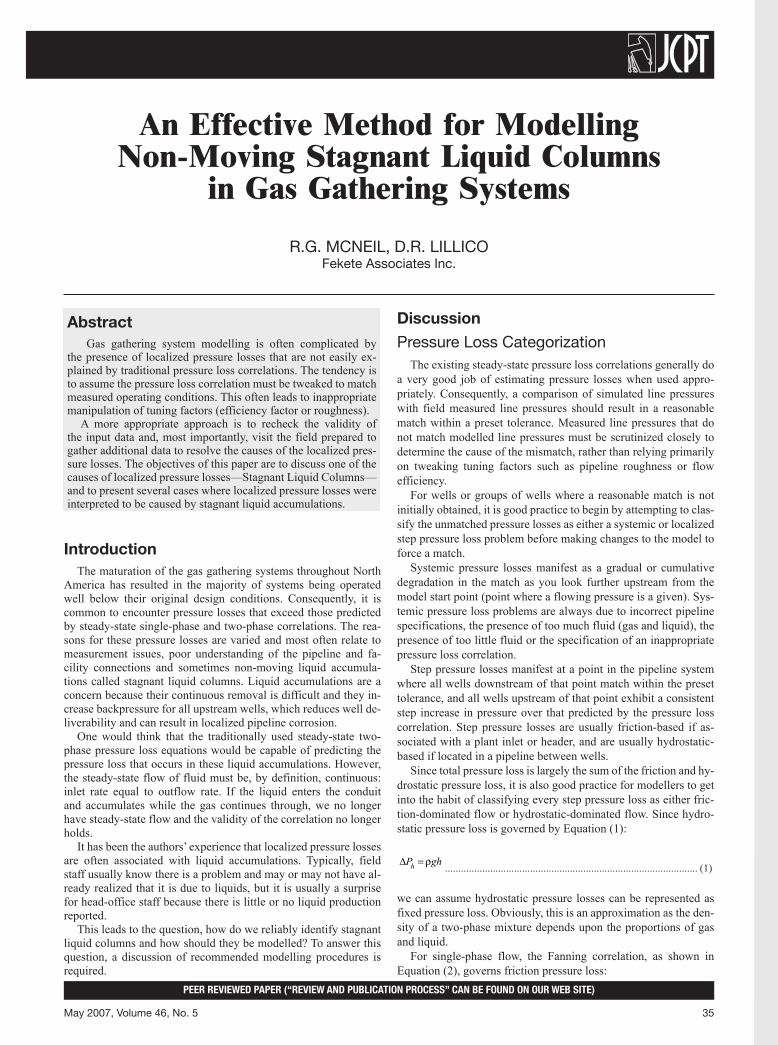
It has long been understood that non-moving liquid in pipelines accumulate in the valleys, river crossings and any place in the ter-rain where the fluid can run downhill and then must be lifted by the gas up the hill on the other side. As gas velocity declines, it is less able the move the liquids out of the trap. Figure 3 presents a sche-matic interpretation of what this scenario may look like.

Since the flow of liquid and gas is uphill out of the trap, and the angle of inclination can be quite severe, it was theorized that per-haps the Turner correlation could be used to predict the gas velocity required to move liquids out of the trap. Since the angle of inclina-tion can vary widely from close to horizontal up to near vertical, it is expected that it would not be as accurate as it is for wellbores. A modified version of the Turner correlation, plotting velocity vs. pipeline operating pressure, is included as Figure 4. In this plot, the upper solid line is the Turner velocity whereas the lower dashed line is the lower limit for effective two-phase flow assuming a min-imum upward angle of inclination of 10 to 20 degrees. The lower dashed line is largely experience-based. The graph has been further annotated to indicate where a stagnant liquid column will occur, where it may occur and where it is not expected.

Use of a Stagnant liquid columnStagnant liquid columns can occur in systems where there is no

apparent liquid production and in systems with known liquid pro-duction. Regardless, this technique should only ever be used if the following tests are passed. The current rules employed are:

1. There must be a significant localized pressure loss over and above that predicted by the pressure correlations. This is also often identified in gathering systems as a step change in pressure.

2. There must be a creek, river crossing or some place where the liquids must first flow downhill and then flow uphill. The up-hill angle should be at least a 20 degree above horizontal.

3. The velocity of the gas is insufficient to move the liquids ef-fectively, as determined from Turner et al.’s chart (Figure 4) as modified for pipeline systems.

4. The measured pressure step change must not exceed 6 kPa/m (0.265 psi/ft) × h, where h is the uphill flow eleva-tion change.

example casesExample 1

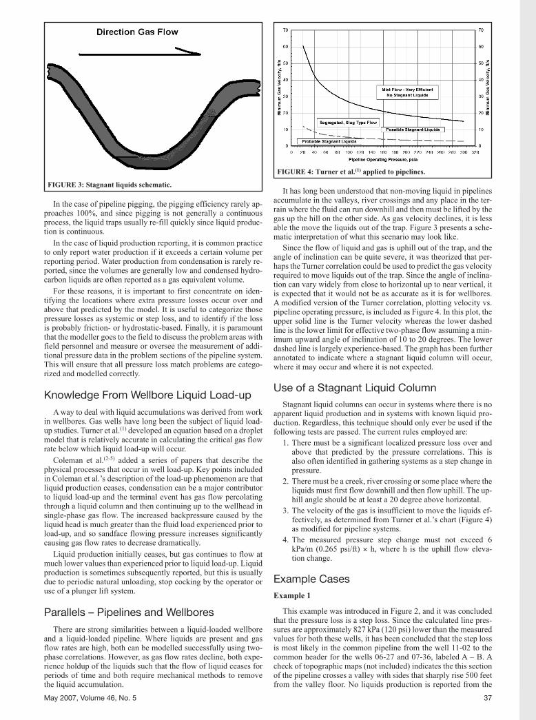
This example was introduced in Figure 2, and it was concluded that the pressure loss is a step loss. Since the calculated line pres-sures are approximately 827 kPa (120 psi) lower than the measured values for both these wells, it has been concluded that the step loss is most likely in the common pipeline from the well 11-02 to the common header for the wells 06-27 and 07-36, labeled A – B. A check of topographic maps (not included) indicates the this section of the pipeline crosses a valley with sides that sharply rise 500 feet from the valley floor. No liquids production is reported from the

FIGURE 4: Turner et al.(1) applied to pipelines.

FIGURE 3: Stagnant liquids schematic.

38 Journal of canadian Petroleum Technology

wells 06-27 and 07-36, but discussion with the operators indicate that the presence of liquids is likely.

The superficial gas velocity for the pipeline segment A – B shown in Figure 2 is less than 0.3 m/s (1 ft/s). From Figure 2, it can seen the lowest pipeline operating pressure is just over 3,447 kPa (500 psia) and the highest operating pressure is approximately 4,137 kPa (600 psia). Although these pressures are higher than the scale shown in the modified Turner et al. graph shown in Figure

4, it is clear that gas velocity of 0.3 m/s (1 ft/s) is very close to or below the lower line indicating liquids will accumulate and steady-state two-phase flow will not occur.

Consequently, a fixed pressure loss of 827 kPa (120 psi) is added to the model between A – B, shown in Figure 5, to model the hydrostatic nature of this pressure loss. The calculated line pressures at the wells 06-27 and 07-36 now match the measured line pressures quite closely. This method replicates the pressure

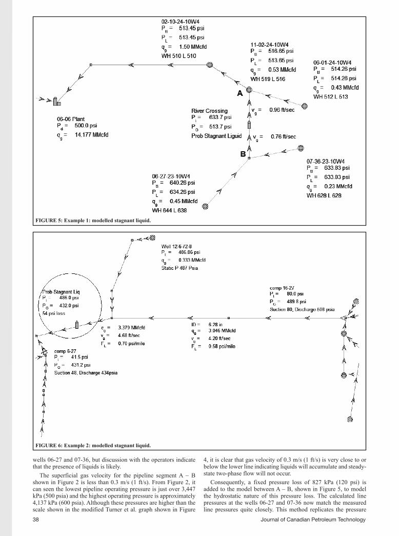
FIGURE 6: Example 2: modelled stagnant liquid.

FIGURE 5: Example 1: modelled stagnant liquid.

May 2007, Volume 46, No. 5 39

loss behaviour commonly experienced when gas flow rates change in pipeline segments operating well below their flow capacity.

If this pipeline segment had been matched using friction-based tuning methods, then any increase in gas flow rate would have re-sult in an extremely large increase in pressure loss in the pipeline, and any decrease in gas flow rate would result in a large decrease in pressure loss. The authors have never modelled a pipeline segment where small changes in gas flow rate resulted in large swings in pressure loss in pipeline segments operating well below their flow capacity.

Example 2

Figure 6 presents another case where a stagnant liquid issue requiring a 372 kPa (54 psi) pressure loss was identified. In this

case, the operator argued that the line had been pigged and was dry. On further questioning, it was determined that the line was last pigged several years previously. The line was subsequently pigged and a large volume of hydrocarbon condensate was recovered. Total gas rates from upstream wells also increased by over 28.31 m3/d (1 MMscfd).

Example 3

Figure 7 presents a case run using a single-phase correlation. Comparison of calculated and measured line pressures demon-strates there is no match. It is known that liquid production is oc-curring in this system. A check on gas velocities [generally > 6 m/s (20 ft/s)] indicates that the use of a two-phase correlation and the input of appropriate elevation changes may resolve the match.

FIGURE 7: Example 3: modelled using single-phase correlation; no match.

FIGURE 8: Example 3: modelled using two-phase correlation; good match.

40 Journal of canadian Petroleum Technology

Figure 8 presents the same case after the input of liquid rates, the input of elevation changes and the switch to a two-phase cor-relation. The match is much improved and considered reasonable given the accuracy of the measurements. A field trip may serve to tighten this match.

ConclusionsA modelling process has been outlined that simplifies the mod-

elling of pipelines systems by stressing the categorization of measured pressure losses as systemic or step loss and then into friction-based or hydrostatic-based. Issues identified by this pro-cess are then resolved via a targeted field trip by the modeller.

In cases where very little liquid or no liquid production occurs, an important cause of pressure loss is stagnant or non-moving liquid columns that are not handled by current pressure loss corre-lations. It is recommended that, once confirmed, liquid accumula-tions can be reasonably modelled as fixed pressure losses.

The method of stagnant liquid columns is a definite improve-ment on the tendency of modellers to use friction-based tuning methods to match measured pressure losses, even though it is an approximation. Further work needs to be done to more accurately describe the phenomenon of stagnant liquids and to explain its im-pact on gas gathering system analysis.

SI Metric Conversion Factorsin × 2.540 E + 00 = cmft × 3.048 E + 00 = mpsi × 6.895 E + 00 = kPa(˚F – 32 ) × 0.55 E + 00 = ˚Cbbl × 1.589 873 E - 01 = m3

MMscfd × 28,317 E + 00 = m3/dft/s × 0.3048 E + 00 = m/s

NoMeNclATUReD = pipeline internal diameterg = gravitational constanth = vertical height of fluid columnL = length of pipelinev = fluid velocityf = Fanning friction factorΔPf = friction pressure lossΔPh = hydrostatic pressure lossρ = fluid density

ReFeReNceS 1. TuRNER, R.G., HuBBARd, M.G. and duKLER, A.E., Analysis

and Prediction of Minimum Flow Rate for the Continuous Removal of Liquids from Gas Wells; Journal of Petroleum Technology, Vol. 246, pp. 1475-1482, November 1969.

2. COLEMAN, S.B., CLAy, H.B., MCCuRdy, d.G. and NORRIS, III, H.L., A New Look at Predicting Gas-Well Load-up; Journal of Pe-troleum Technology, Vol. 43, No. 3, pp. 329-333, March 1991.

3. COLEMAN, S.B., CLAy, H.B., MCCuRdy, d.G. and NORRIS, III, H.L., understanding Gas-Well Load-up Behaviour; Journal of Pe-troleum Technology, Vol. 43, No. 3, pp. 334-338, March 1991.

4. COLEMAN, S.B., CLAy, H.B., MCCuRdy, d.G. and NORRIS, III, H.L., The Blowdown-Limit Model; Journal of Petroleum Tech-nology, Vol. 43, No. 3, pp. 339-343, March 1991.

5. COLEMAN, S.B., CLAy, H.B., MCCuRdy, d.G. and NORRIS, III, H.L., Applying Gas-Well Load-up Technology; Journal of Petro-leum Technology, Vol. 43, No. 3, pp. 344-349, March 1991.

Further Reading

1. BEGGS, H.d. and BRILL, J.P., A Study of Two-Phase Flow in In-clined Pipes; Journal of Petroleum Technology, pp. 607-617, May 1973.

2. MATTAR, L. and ZAORAL, K., Gas Pipeline Efficiencies and Pres-sure Gradient Curves; paper No. 84-35-93 presented at the 35th Annual Technical Meeting of the Petroleum Society of CIM, Calgary, AB, 10-13 June 1984.

3. MCNEIL, R.G., A Procedure for Modelling Gas Gathering Systems; Journal of Canadian Petroleum Technology, Vol. 40, No. 1, pp. 7-10, January 2001.

4. yOuNG, J., MCNEIL, R. and KNIBBS, J., Case Study: Including the Effects of Stagnant Water in Gas Gathering System Modelling; Paper SPE 75946 presented at the SPE Gas Technology Symposium, Calgary, AB, 30 April – 02 May 2002.

Provenance—Original Petroleum Society manuscript, An Effective Method for Modelling Non-Moving “Stagnant” Liquid Columns in Gas Gathering Systems (2004-175), first presented at the 5th Canadian International Petroleum Conference (the 55th Annual Technical Meeting of the Petroleum Society), June 8-10, 2004, in Calgary, Alberta. Ab-stract submitted for review december 9, 2003; editorial comments sent to the author(s) <editorial sent>; revised manuscript received March 30, 2007; paper approved for pre-press March 30, 2007; final approval April 7, 2007.

Authors’ BiographiesRalph McNeil has been with Fekete since 1987, where he worked in reserve evalu-ations and pipeline optimization before assuming the role of Senior Technical Ad-visor responsible for the development of F.A.S.T. Piper™. He has taught the F.A.S.T. Piper™ course for over 10 years and is well practiced in converting complicated pipe-line problems into manageable, solvable components.

Dave Lillico has been with Fekete since 1989, where he worked in reserve evalua-tions until 1999 at which time he assumed the role of manager of the Pipeline Optimi-zation group. dave has been involved with modelling all aspects of gas flow from the reservoir through the wellbore, pipelines and compression. dave has modelled gath-ering systems throughout North America, Australia, Bangladesh, Tanzania and Turkey. The pipeline modelling group that

dave supervises is responsible for modelling in excess of 15,000 wells/year.