An EDF-based Scheduling Algorithm for …anderson/papers/euro05a.pdfAn EDF-based Scheduling...
22
An EDF-based Scheduling Algorithm for Multiprocessor Soft Real-Time Systems * James H. Anderson, Vasile Bud, and UmaMaheswari C. Devi Department of Computer Science The University of North Carolina at Chapel Hill Abstract We consider the use of the earliest-deadline-first (EDF) scheduling algorithm in soft real-time multiproces- sor systems. In hard real-time systems, a significant disparity exists between EDF-based schemes and Pfair scheduling (which is the only known way of optimally scheduling recurrent real-time tasks on multiprocessors): on M processors, all known EDF variants have utilization-based schedulability bounds of approximately M/2, while Pfair algorithms can fully utilize all processors. This is unfortunate because EDF-based algorithms entail lower scheduling and task-migration overheads. In work on hard real-time systems, it has been shown that this disparity in schedulability can be lessened by placing caps on per-task utilizations. In this paper, we show that it can also be lessened by easing the requirement that all deadlines be met. Our main contribution is a new EDF-based scheme that ensures bounded deadline tardiness. In this scheme, per-task utilizations must be capped, but overall utilization need not be restricted. The required cap is quite liberal. Hence, our scheme should enable a wide range of soft real-time applications to be scheduled with no constraints on total utilization . We also propose techniques and heuristics that can be used to reduce tardiness. To the best of our knowledge, this paper is the first to examine multiprocessor EDF scheduling in the context of soft real-time systems. Keywords: Multiprocessor systems, soft real-time, earliest-deadline-first scheduling. * Work supported by NSF grants CCR 0204312, CCR 0309825, and CCR 0408996. The third author was also supported by an IBM Ph.D. fellowship.
Transcript of An EDF-based Scheduling Algorithm for …anderson/papers/euro05a.pdfAn EDF-based Scheduling...

An EDF-based Scheduling Algorithm for Multiprocessor
Soft Real-Time Systems∗
James H. Anderson, Vasile Bud, and UmaMaheswari C. Devi
Department of Computer Science
The University of North Carolina at Chapel Hill
Abstract
We consider the use of the earliest-deadline-first (EDF) scheduling algorithm in soft real-time multiproces-
sor systems. In hard real-time systems, a significant disparity exists between EDF-based schemes and Pfair
scheduling (which is the only known way of optimally scheduling recurrent real-time tasks on multiprocessors):
on M processors, all known EDF variants have utilization-based schedulability bounds of approximately M/2,
while Pfair algorithms can fully utilize all processors. This is unfortunate because EDF-based algorithms entail
lower scheduling and task-migration overheads. In work on hard real-time systems, it has been shown that
this disparity in schedulability can be lessened by placing caps on per-task utilizations. In this paper, we show
that it can also be lessened by easing the requirement that all deadlines be met. Our main contribution is a
new EDF-based scheme that ensures bounded deadline tardiness. In this scheme, per-task utilizations must be
capped, but overall utilization need not be restricted. The required cap is quite liberal. Hence, our scheme
should enable a wide range of soft real-time applications to be scheduled with no constraints on total utilization.
We also propose techniques and heuristics that can be used to reduce tardiness. To the best of our knowledge,
this paper is the first to examine multiprocessor EDF scheduling in the context of soft real-time systems.
Keywords: Multiprocessor systems, soft real-time, earliest-deadline-first scheduling.
∗Work supported by NSF grants CCR 0204312, CCR 0309825, and CCR 0408996. The third author was also supported by an IBMPh.D. fellowship.
1 Introduction
Real-time multiprocessor systems are now commonplace. Designs range from single-chip architectures, with a
modest number of processors, to large-scale signal-processing systems, such as synthetic-aperture radar systems. In
recent years, scheduling techniques for such systems have received considerable attention. In an effort to catalogue
these various techniques, Carpentar et al. [4] suggested the categorization shown in Table 1, which pertains to
scheduling schemes for periodic or sporadic tasks systems. In such systems, each task is invoked repeatedly, and
each such invocation is called a job. The table classifies scheduling schemes along two dimensions:
1. Complexity of the priority mechanism. Along this dimension, scheduling disciplines are categorized
according to whether task priorities are (i) static, (ii) dynamic but fixed within a job, or (iii) fully-dynamic.
Common examples of each type include (i) rate-monotonic (RM) [6], (ii) earliest-deadline-first (EDF) [6], and
(iii) least-laxity-first (LLF) [8] scheduling.
2. Degree of migration allowed. Along this dimension, disciplines are ranked as follows: (i) no migration
(i.e., task partitioning), (ii) migration allowed, but only at job boundaries (i.e., dynamic partitioning at the
job level), and (iii) unrestricted migration (i.e., jobs are also allowed to migrate).
The entries in Table 1 give known schedulable utilization bounds for each category, assuming that jobs can be
preempted and resumed later. If U is a schedulable utilization for an M -processor scheduling algorithm A, then
A can correctly schedule any set of periodic (or sporadic) tasks with total utilization at most U on M processors.
The top left entry in the table means that there exists some algorithm in the unrestricted-migration/static-priority
class that can correctly schedule every task set with total utilization at most M2
3M−2 , and that there exists some
task set with total utilization slightly higher than M+12 that cannot be correctly scheduled by any algorithm in the
same class. The other entries in the table have a similar interpretation.
According to Table 1, scheduling algorithms from only one category can schedule tasks correctly with no
utilization loss, namely, algorithms that allow full migration and use fully-dynamic priorities (the top right entry).
The fact that it is possible for algorithms in this category to incur no utilization loss follows from work on scheduling
algorithms that ensure proportionate fairness (Pfairness) [3]. Pfair algorithms break tasks into smaller uniform
pieces called “subtasks,” which are then scheduled. The subtasks of a task may execute on any processor, i.e.,
tasks may migrate within jobs. Hence, Pfair scheduling algorithms may suffer higher scheduling and migration
overheads than other schemes. Thus, the other categories in Table 1 are still of interest.
In four of the other categories, the term α represents a cap on individual task utilizations. Note that, if
such a cap is not exploited, then the upper bound on schedulable utilization for each of the other categories is
1

3: full migration M23M−2 ≤ U ≤ M+1
2 U ≥ M − α(M − 1), if α ≤ 12 U = M
M22M−1 ≤ U ≤ M+1
2 , otherwise
2: restricted migration U ≤ M+12 U ≥ M − α(M − 1), if α ≤ 1
2 U ≥ M − α(M − 1), if α ≤ 12
M − α(M − 1) ≤ U ≤ M+12 M − α(M − 1) ≤ U ≤ M+1
2,otherwise ,otherwise
1: partitioned (√
2− 1)M ≤ U ≤ M+1
1+21
M+1U = βM+1
β+1 , where β =j
1α
kU = M+1
2
1: static 2: job-level dynamic 3: fully dynamic
Table 1: Known lower and upper bounds on schedulable utilization (denoted U) for the different classes of preemp-tive scheduling algorithms.
approximately M/2 or lower. This is no accident: as shown in [4], no algorithm in these categories can successfully
schedule all task systems with total utilization at most B on M processors, where (M + 1)/2 < B ≤ M . Given the
scheduling and migration overheads of Pfair algorithms, the disparity in schedulability between Pfair algorithms
and those in other categories is somewhat disappointing.
Fortunately, as the table suggests, if individual task utilizations can be capped, then it is sometimes possible
to significantly relax restrictions on total utilization. For example, in the entries in the middle column, as α
approaches 0, U approaches M . This follows from work on multiprocessor EDF scheduling [1, 2, 7], which shows
that an interesting “middle ground” exists between unrestricted EDF-based algorithms (which have upper bounds of
approximately M/2 on schedulable utilization) and Pfair algorithms (which have a schedulable utilization bound of
M). In essence, establishing this middle ground involved addressing the following question: if per-task utilizations
are restricted, and if no deadlines can be missed, then what is the largest overall utilization that can be allowed? In
this paper, we approach this middle ground in a different way by addressing this question: if per-task utilizations are
restricted, but overall utilization is not, then by how much can deadlines be missed? Our interest in this question
stems from the increasing prevalence of applications such as networking, multimedia, and immersive graphics
systems (to name a few) that have only soft real-time requirements.
While we do not yet understand how to answer to the question raised above for any EDF-based scheme, we do
take a first step towards such an understanding in this paper by presenting one such scheme and by establishing
deadline tardiness bounds for it. Our basic scheme adheres to the conditions of the middle entry of Table 1
(restricted migration, job-level dynamic priorities).
The maximum tardiness that any task may experience in our scheme is dependent on the per-task utilization cap
assumed—the lower the cap, the lower the tardiness threshold. Even with a cap as high as 0.5 (half of the capacity
2

of one processor), reasonable tardiness bounds can be guaranteed for a significant percentage of task systems. (In
contrast, if α = 0.5 in the middle entry of Table 1, then approximately 50% of the system’s overall capacity may be
lost.) Hence, our scheme should enable a wide range of soft real-time applications to be scheduled in practice with
no constraints on total utilization. In addition, when a job misses its deadline, we do not require a commensurate
delay in the release of the next job of the same task. As a result, each task’s required processor share is maintained
in the long term. Our scheme has the additional advantage of limiting migration costs, even in comparison to other
EDF-based schemes: only up to M − 1 tasks, where M is the number of processors, ever migrate, and those that
do, do so only between jobs. As noted in [4], migrations between jobs should not be a serious concern in systems
where little per-task state is carried over from one job to the next.
The rest of this paper is organized as follows. In Sec. 2, our system model is presented. In Sec. 3 our proposed
algorithm is described and a tardiness bound is derived for it. Techniques and heuristics that can be used to
reduce tardiness observed in practice are presented in Sec. 4. In Sec. 5, a simulation-based evaluation of our basic
algorithm and proposed heuristics is presented. Finally, we conclude in Sec. 6.
2 System Model
We consider the scheduling of a recurrent (periodic or sporadic) task system τ comprised of N tasks on M identical
processors. The kth processor is denoted Pk, where 1 ≤ k ≤ M . Each task Ti, where 1 ≤ i ≤ n, is characterized
by a period pi, an execution cost ei ≤ pi, and a relative deadline di. Each task Ti is invoked at regular intervals,
and each invocation is referred to as a job of Ti. The kth job of Ti is denoted Ti,k. The first job may be invoked
or released at any time at or after time zero and the release times of any two consecutive jobs of Ti should differ
by at least pi time units. If every two consecutive job releases differ by exactly pi time units, then Ti is said to be
a periodic task; otherwise, Ti is a sporadic task. Every job of Ti has a worst-case execution requirement of ei time
units and an absolute deadline given by the sum of its release time and its relative deadline, di. In this paper, we
assume that di = pi holds, for all i. We sometimes use the notation Ti(ei, pi) to concisely denote the execution cost
and period of task Ti.
The utilization of task Ti is denoted ui and is given by ei/pi. If ui ≤ 1/2, then Ti is called a light task . In
this paper, we assume that every task to be scheduled is light. Because a light task can consume up to half the
capacity of a single processor, we do not expect this to be a restrictive assumption in practice. The total utilization
of a task system τ is defined as Usum(τ) =∑n
i=1 ui. A task system is said to fully utilize the available processing
capacity if its total utilization equals the number of processors (M). The maximum utilization of any task in τ is
denoted umax(τ). A task system is preemptive if the execution of its jobs may be interrupted and resumed later.
3

In this paper, we consider only preemptive scheduling policies. We also place no constraints on total utilization.
The jobs of a soft real-time task may occasionally miss their deadlines, if the amount by which a job misses its
deadline, referred to as its tardiness, is bounded. Formally, the tardiness of a job Ti,j in schedule S is defined as
tardiness(Ti,j ,S) = max(0, t− ta), where t is the time at which Ti,j completes executing in S and ta is its absolute
deadline. The tardiness of a task system τ under scheduling algorithm A, denoted tardiness(τ,A), is defined as the
maximum tardiness of any job in τ under any schedule under A. If κ is the maximum tardiness of any task system
under A, then A is said to ensure a tardiness bound of κ. Though tasks in a soft real-time system are allowed to
have nonzero tardiness, we assume that missed deadlines do not delay future job releases. That is, if a job of a task
misses its deadline, then the release time of the next job of that task remains unaltered. Of course, we assume that
consecutive jobs of the same task cannot be scheduled in parallel. Thus, a missed deadline effectively reduces the
interval over which the next job should be scheduled in order to meet its deadline.
Our goal in this paper is to derive an EDF-based multiprocessor scheduling scheme that ensures bounded
tardiness. In a “pure” EDF scheme, jobs with earlier deadlines would (always) be given higher priority. In our
scheme, this is usually the case, but (as explained later) certain tasks are treated specially and are prioritized using
other rules. Because we do not delay future job releases when a deadline is missed, our scheme ensures (over the
long term) that each task receives a processor share approximately equal to its utilization. Thus, it should be useful
in settings where maintaining correct share allocations is more important than meeting every deadline. In addition,
schemes that ensure bounded tardiness are useful in systems in which a utility function is defined for each task [5].
Such a function specifies the “value” or usefulness of the current job of a task as a function of time; beyond a job’s
deadline, its usefulness typically decays from a positive value to 0 or below. The amount of time after its deadline
beyond which the completion of a job has no value implicitly specifies a tardiness threshold for the corresponding
task.
3 Algorithm EDF-fm
In this section, we propose Algorithm EDF-fm (fm denotes that each task is either fixed or migrating), an EDF-based
multiprocessor scheduling algorithm that ensures bounded tardiness for task systems whose per-task utilizations
are at most 1/2. EDF-fm does not place any restrictions on the total system utilization. Further, at most M − 1
tasks need to be able to migrate, and each such task migrates between two processors, across job boundaries only.
This has the benefit of lowering the number of tasks whose states need to be stored on a processor and the number
of processors on which each task’s state needs to be stored. Also, the runtime context of a job, which can be
expected to be larger than that of a task, need not be transferred between processors.
4
EDF-fm consists of two phases: an assignment phase and an execution phase. The assignment phase executes
offline and consists of sequentially assigning each task to one or two processors. In the execution phase, jobs are
scheduled for execution at runtime such that over reasonable intervals (as explained later), each task executes at
a rate that is commensurate with its utilization. The two phases are explained in detail below. The following
notation shall be used.
si,jdef= Percentage of Pj ’s processing capacity (expressed as a fraction) allocated to Ti, 1 ≤ i ≤ n, 1 ≤ j ≤ M .
(Ti is said to have a share of si,j on Pj .) (1)
fi,jdef=
si,j
ui, the fraction of Ti’s total execution requirement that Pj can handle, 1 ≤ i ≤ n, 1 ≤ j ≤ M. (2)
3.1 Assignment Phase
The assignment phase represents a mapping of tasks to processors. Each task is assigned to either one or two
processors. Tasks assigned to two processors are called migrating tasks, while those assigned to only one processor
are called fixed or non-migrating tasks. A fixed task Ti is assigned a share, si,j , equal to its utilization ui on the only
processor Pj to which it is assigned. A migrating task has shares on both processors to which it is assigned. The
sum of its shares equals its utilization. The assignment phase of EDF-fm also ensures that at most two migrating
tasks are assigned to any processor.
In Fig. 1, a task-assignment algorithm, denoted Assign-Tasks, is given that satisfies the following properties
for any task set τ with umax(τ) ≤ 1/2 and Usum(τ) ≤ M .
(P1) Each task is assigned shares on at most two processors only. A task’s total share equals its utilization.
(P2) Each processor is assigned at most two migrating tasks only and may be assigned any number of fixed tasks.
(P3) The sum of the shares allocated to the tasks on any processor is at most one.
In the pseudo-code for this algorithm, the ith element u[i] of the global array u represents the utilization ui of
task Ti, s[i][j] denotes si,j (as defined in (1)), array p[i] contains the processor(s) to which task i is assigned, and
arrays m[i] and f [i] denote the migrating tasks and fixed tasks assigned to processor i, respectively. Note that p[i]
and m[i] are each vectors of size two.
Algorithm Assign-Tasks assigns tasks in sequence to processors, starting from the first processor. Tasks and
processors are both considered sequentially. Local variables proc and task denote the current processor and task,
respectively. Tasks are assigned to proc as long as the processing capacity of proc is not exhausted. If the current
task task cannot receive its full share of utask from proc, then part of the processing capacity that it requires is
5
Algorithm Assign-Tasks()
global var
u : array [1..N ] of double initially 0.0;
s : array [1..N ][1..M ] of double initially 0.0;
p : array [1..N ][1..2] of 0..M initially 0;
m: array [1..M ][1..2] of 0..N initially 0;
f : array [1..M ][1..N ] of 0..N initially 0
local var
proc : 1..M initially 1;
task : 1..N ;
AvailUtil : double;
mt, ft : integer initially 0
1 AvailUtil := 1.0;
2 for task := 1 to n do
3 if AvailUtil ≥ u[task ] then
4 s[task ][proc] := u[task ];
5 AvailUtil := AvailUtil − u[task ];
6 ft := ft + 1;
7 p[task ][1] := proc;
8 f [proc][ft] := task
else
9 if AvailUtil > 0 then
10 s[task ][proc] := AvailUtil ;
11 mt := mt + 1;
12 m[proc][mt] := task ;
13 p[task ][1], p[task ][2] := proc, proc + 1;
14 mt, ft := 1, 0;
15 m[proc + 1][mt] := task
else
16 mt, ft := 0, 1;
17 p[task ][1] := proc + 1;
18 f [proc + 1][ft] := task
fi
19 proc := proc + 1;
20 s[task ][proc] := u[task ]− s[task ][proc − 1];
21 AvailUtil := 1− s[task ][proc]
fi
od
Figure 1: Algorithm Assign-Tasks.
allocated on the next processor, proc+1, such that the sum
of the shares allocated to task on the two processors equals
utask. It is easy to see that assigning tasks to processors
following this simple approach satisfies (P1)–(P3).
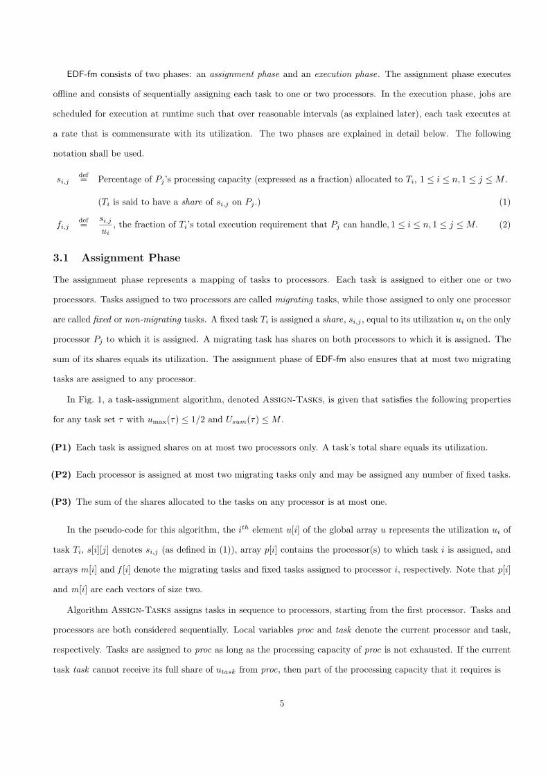
Example task assignment. Consider a task set τ com-
prised of nine tasks: T1(5, 20), T2(3, 10), T3(1, 2), T4(2, 5),
T5(2, 5), T6(1, 10), T7(2, 5), T8(7, 20), and T9(3, 10). The
total utilization of this task set is three. A share assign-
ment produced by Assign-Tasks is shown in Fig. 2. In
this assignment, T3 and T7 are migrating tasks; the remain-
ing tasks are fixed. T3 has a share of 920 on processor P1
and a share of 120 on processor P2, while T7 shares of 1
20
and 720 on processors P2 and P3, respectively.
3.2 Execution Phase
Having devised a way of assigning tasks to processors, the
next step is to devise an online scheduling algorithm that
is easy to analyze and ensures bounded tardiness. For a
fixed task, we merely need to decide when to schedule each
of its jobs on its (only) assigned processor. For a migrating
task, we must decide both when and where its jobs should
execute. Before describing our scheduling algorithm, we
discuss some considerations that led to its design.
In order to analyze a scheduling algorithm and for the
algorithm to guarantee bounded tardiness, it should be
possible to bound the total demand for execution time by
all tasks on each processor over well-defined time intervals.
We first argue that bounding total demand may not be possible if the jobs of migrating tasks are allowed to miss
their deadlines.
Because a deadline miss of a job does not lead to a postponement of the release times of subsequent jobs of the
6
Processor P2
s4,2 = 25
s3,2 = 120
s5,2 = 25
s6,2 = 110
s7,2 = 120
Processor P3
s7,3 = 720
s8,3 = 720
s9,3 = 310
Processor P1
s3,1 = 920
s2,1 = 310
s1,1 = 520
Figure 2: Example task assignment on three processors using
Algorithm Assign-Tasks.
same task, and because two jobs of a task may not ex-
ecute in parallel, the tardiness of a job of a migrating
task executing on one processor can affect the tardi-
ness of its successor job, which may otherwise execute
in a timely manner on a second processor. In the worst
case, the second processor may be forced to idle. The
tardiness of the second job may also impact the timeli-
ness of fixed tasks and other migrating tasks assigned
to the same processor, which in turn may lead to dead-
line misses of both fixed and migrating tasks on other processors or unnecessary idling on other processors.
As a result, a set of dependencies is created among the jobs of migrating tasks, resulting in an intricate linkage
among processors that complicates scheduling analysis. It is unclear how per-processor demand can be precisely
bounded when activities on different processors become interlinked.
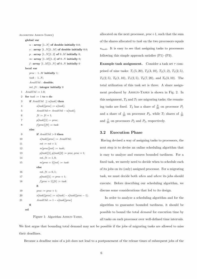
Let us look at a concrete example that reveals this linkage among processors. Consider task set τ , introduced
earlier, with task assignments and processor shares shown in Fig. 2. For simplicity, assume that the execution of
the jobs of a migrating task alternate between the two processors to which the task is assigned. T3 releases its first
job on P1, while T7 releases its first job on P3. (We are assuming such a naıve assignment pattern to illustrate
the processor linkage using a short segment of a real schedule. Such a linkage occurs even with an intelligent
job-assignment pattern if migrating tasks miss their deadlines.) A complete schedule up to time 27, with the jobs
assigned to each processor scheduled using EDF, is shown in Fig. 3.
In Fig. 3, the sixth job of the migrating task T3 misses its deadline (at time 12) on P2 and completes executing
at time 14. This prevents the next job of T3 released on P1 from being scheduled until time 14 and it misses its
deadline. Recall that a deadline miss does not cause future job releases to be postponed, thus the seventh job of
T3 is released at time 12 and has a deadline at time 14.
The missed deadlines of the migrating task T3 impact the execution of the fixed tasks on P2 also. The deadline
misses of the fixed tasks T4, T5, and T6 cause deadline misses of the migrating task T7 on P2. As a result, the
fourth job of T7 misses its deadline, which in turn reduces the interval over which the fifth job of the same task can
execute on P3. Thus, a nontrivial linkage is established among the processors that impacts system tardiness.
Per-processor scheduling rules. EDF-fm eliminates this linkage among processors by ensuring that migrating
tasks do not miss their deadlines. Jobs of migrating tasks are assigned to processors using static rules that are
independent of runtime dynamics. The jobs assigned to a processor are scheduled independently of other processors,
7

T (5,20)1
T (3,10)2
P1
P3
P2
P1
P2
T (7,20)8
T (3,10)9
P3
0 2 4 6 8 10 12 14 16 18 20 22 24 26 time
��������
��������
��������
��������
��������
��������
��������
��������
tard
T (1,10)6 ��������
��������
��������
��������
tard tard
T (2,5)5��������
��������
��������
��������
��������
��������
��������
��������
��������
��������
��������
��������
��������
��������
��������
��������
tard tard tard
T (2,5)4��������
��������
��������
��������
��������
��������
��������
��������
��������
��������
��������
��������
��������
��������
��������
��������
tard tard
T (1,2)3
T (2,5)7
��������
��������
������
������
������
������
������
������
������
������
������
������
tard
Allocations on
MissedDeadline
tard tardiness
tard tard tard
tard
Figure 3: Illustration of processor linkage.
and on each processor, migrating tasks are statically prioritized over fixed tasks. Jobs within each task class are
scheduled using EDF, which is optimal on uniprocessors. This priority scheme, together with the restriction that
migrating tasks have utilizations at most 1/2, and the task assignment property (from (P2)) that there are at
most two migrating tasks per processor, ensures that migrating tasks never miss their deadlines. Therefore, the
jobs of migrating tasks executing on different processors do not impact one another, and each processor can be
analyzed independently. Thus, the multiprocessor scheduling analysis problem at hand is transformed into a simpler
uniprocessor one.
In the description of EDF-fm, we are left with defining rules that map jobs of migrating tasks to processors. A
naıve assignment of the jobs of a migrating task to its processors can cause an over-utilization on one of its assigned
processors. EDF-fm follows a job assignment pattern that prevents over-utilization in the long run by ensuring
that over well-defined time intervals (explained later), the demand due to a migrating task on each processor is in
accordance with its allocated share on that processor.
For example, consider the migrating task T7(2, 5) in the example above. T7 has a share of s7,2 = 120 on P2 and
s7,3 = 720 on P3. Also, f7,2 = s7,2
u7= 1
8 and f7,3 = s7,3u7
= 78 , which imply that P2 and P3 should be capable of
executing 18 and 7
8 of the workload of T7, respectively. Our goal is to devise a job assignment pattern that would
ensure that in the long run, the fraction of a migrating task Ti’s workload executed on Pj is close to fi,j . One
8
T7,2 T7,7 T7,12 T7,13 T7,14 T7,15
T7,16
T7,4 T7,5T7,1 T7,6
T7,8
T7,9 T7,10 T7,11T7,3
time
0 5 10 15 20 25 30 35 40 45 50 55 60 65 70 75 80
Jobs assigned to
Jobs assignedto P3
P2
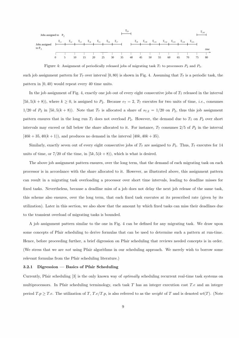
Figure 4: Assignment of periodically released jobs of migrating task T7 to processors P2 and P3.
such job assignment pattern for T7 over interval [0, 80) is shown in Fig. 4. Assuming that T7 is a periodic task, the
pattern in [0, 40) would repeat every 40 time units.
In the job assignment of Fig. 4, exactly one job out of every eight consecutive jobs of T7 released in the interval
[5k, 5(k + 8)), where k ≥ 0, is assigned to P2. Because e7 = 2, T7 executes for two units of time, i.e., consumes
1/20 of P2 in [5k, 5(k + 8)). Note that T7 is allocated a share of s7,2 = 1/20 on P2, thus this job assignment
pattern ensures that in the long run T7 does not overload P2. However, the demand due to T7 on P2 over short
intervals may exceed or fall below the share allocated to it. For instance, T7 consumes 2/5 of P2 in the interval
[40k + 35, 40(k + 1)), and produces no demand in the interval [40k, 40k + 35).
Similarly, exactly seven out of every eight consecutive jobs of T7 are assigned to P3. Thus, T7 executes for 14
units of time, or 7/20 of the time, in [5k, 5(k + 8)), which is what is desired.
The above job assignment pattern ensures, over the long term, that the demand of each migrating task on each
processor is in accordance with the share allocated to it. However, as illustrated above, this assignment pattern
can result in a migrating task overloading a processor over short time intervals, leading to deadline misses for
fixed tasks. Nevertheless, because a deadline miss of a job does not delay the next job release of the same task,
this scheme also ensures, over the long term, that each fixed task executes at its prescribed rate (given by its
utilization). Later in this section, we also show that the amount by which fixed tasks can miss their deadlines due
to the transient overload of migrating tasks is bounded.
A job assignment pattern similar to the one in Fig. 4 can be defined for any migrating task. We draw upon
some concepts of Pfair scheduling to derive formulas that can be used to determine such a pattern at run-time.
Hence, before proceeding further, a brief digression on Pfair scheduling that reviews needed concepts is in order.
(We stress that we are not using Pfair algorithms in our scheduling approach. We merely wish to borrow some
relevant formulas from the Pfair scheduling literature.)
3.2.1 Digression — Basics of Pfair Scheduling
Currently, Pfair scheduling [3] is the only known way of optimally scheduling recurrent real-time task systems on
multiprocessors. In Pfair scheduling terminology, each task T has an integer execution cost T.e and an integer
period T.p ≥ T.e. The utilization of T , T.e/T.p, is also referred to as the weight of T and is denoted wt(T ). (Note
9
that in the context of Pfair scheduling, tasks are denoted using upper-case letters without subscripts.)
Pfair algorithms allocate processor time in discrete quanta that are uniform in size. Assuming that a quantum
is one time unit in duration, the interval [t, t+1), where t is a non-negative integer, is referred to as slot t. At most
one task may execute on each processor in each slot, and each task may execute on at most one processor only in
every slot. The sequence of allocation decisions over time slots defines a schedule S. Formally, S : τ × N 7→ {0, 1}.
S(T, t) = 1 iff T is scheduled in slot t.
The notion of a Pfair schedule for a periodic task T is defined by comparing such a schedule to an ideal fluid
schedule, which allocates wt(T ) processor time to T in each slot. Deviation from the allocation in a fluid schedule
is formally captured by the concept of lag . Formally, the lag of task T at time t in schedule S is the difference
between the total allocations to T in a fluid schedule and S in the interval [0, t), i.e.,
lag(T, t,S) = wt(T ) · t−t−1∑u=0
S(T, u). (3)
A schedule S is said to be Pfair iff
(∀T, t :: −1 < lag(T, t,S) < 1) (4)
holds. Informally, the allocation error associated with each task must always be less than one quantum.
The above constraints on lag have the effect of breaking task T into a potentially infinite sequence of quantum-
length subtasks. The ith subtask of T is denoted Ti, where i ≥ 1. (In the context of Pfair scheduling, Ti does not
denote the ith task, but the ith subtask of task T .)
Each subtask Ti is associated with a pseudo-release r(Ti) and a pseudo-deadline d(Ti) defined as follows:
r(Ti) =⌊
i− 1wt(T )
⌋(5)
d(Ti) =⌈
i
wt(T )
⌉(6)
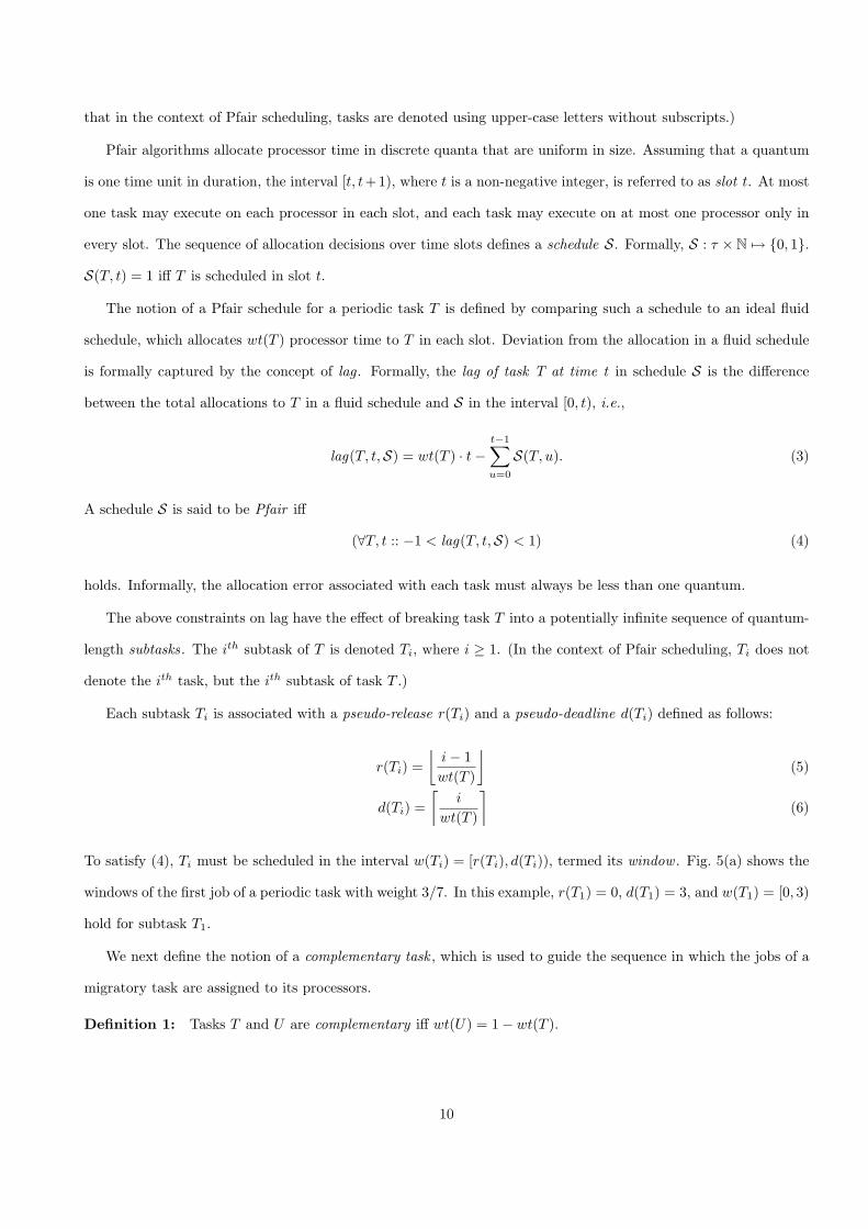
To satisfy (4), Ti must be scheduled in the interval w(Ti) = [r(Ti), d(Ti)), termed its window . Fig. 5(a) shows the
windows of the first job of a periodic task with weight 3/7. In this example, r(T1) = 0, d(T1) = 3, and w(T1) = [0, 3)
hold for subtask T1.
We next define the notion of a complementary task , which is used to guide the sequence in which the jobs of a
migratory task are assigned to its processors.
Definition 1: Tasks T and U are complementary iff wt(U) = 1− wt(T ).
10

T1
T2
T3
U1
U2
U3
U4
0 1 2 3 4 5 76
0 1 2 3 4 5 76
X
X
X
X
X
XT (3/7)
U (4/7)
time
slot
X
(b)
T3
T2
T1
0 1 2 3 4 5 760 1 2 3 4 5 76
timeslot
(a)
Figure 5: (a) Windows of the first job of a periodic task Twith weight 3/7. This job consists of subtasks T1, T2, and T3,each of which must be scheduled within its window. (This pat-tern repeats for every job.) (b) A partial complementary Pfairschedule for a pair of complementary tasks, T and U , on oneprocessor. The slot in which a subtask is scheduled is indicatedby an “X”. In this schedule, every subtask of U is scheduled inthe first slot of its window, while every subtask of T is scheduledin the last slot.
Tasks T and U shown in Fig. 5(b) are complementary
to one another. A partial Pfair schedule for these two
tasks on one processor, in which the subtasks of T are
always scheduled in the last slot of their windows and
those of U in the first slot, is also shown. We call
such a schedule a complementary schedule. It is easy
to show that such a schedule is always possible for two
complementary periodic tasks.
With the above introduction to Pfair scheduling,
we are now ready to present the details of distributing
the jobs of a migrating task between its processors.
3.2.2 Assignment Rules for Jobs of Migrating
Tasks
Let Ti be any migrating periodic task (we later relax the assumption that Ti is periodic) that is assigned shares
si,j and si,j+1 on processors Pj and Pj+1, respectively. (Note that every migrating task is assigned shares on two
consecutive processors by Assign-Tasks.) As explained earlier, fi,j and fi,j+1 (given by (2)) denote the fraction
of the workload (i.e., the total execution requirement) of T that should be executed on Pj and Pj+1, respectively,
in the long run. By (P1), the total share allocated to Ti on Pj and Pj+1 is ui. Hence, by (2), it follows that
fi,j + fi,j+1 = 1. (7)
Assuming that the execution cost and period of every task are rational numbers (that can be expressed as a ratio
of two integers), ui, si,j , and hence, fi,j and fi,j+1 are also rational numbers. Let fi,j = xi,j
yi, where xi,j and yi
are positive integers that are relatively prime. Then, by (7), it follows that fi,j+1 = yi−xi,j
yi. Therefore, one way
of distributing the workload of Ti between Pj and Pj+1 that is commensurate with the shares of Ti on the two
processors would be to assign xi,j out of every yi jobs to Pj and the remaining jobs to Pj+1.
We borrow from the aforementioned concepts of Pfair scheduling to guide in the distribution of jobs. If we let
fi,j and fi,j+1 denote the weights of two fictitious Pfair tasks, V and W , and let a quantum span pi time units, then
the following analogy can be made between the jobs of the migrating task Ti and the subtasks of the fictitious tasks
V and W . First, slot s represents the interval in which the (s + 1)st job of Ti, which is released at the beginning
of slot s, needs to be scheduled. (Recall that slots are numbered starting from 0.) Next, subtask Vg represents the
11
W3
W1
W2
~ ~
V1
W4
W5
V1
W7
W6
W5
W3
W4
W1
W2
0 5 10 15 20 25 30 35 40
W7
W6
T7,5T7,2 T7,3 T7,4 T7,6 T7,7 T7,8 T7,5T7,1 T7,2 T7,3 T7,4 T7,6 T7,7 T7,8T7,1
time
slot
V 72(1/8 = f
W (7/8 = f 73
0 5 10 15 20 25 36 41 46 51
The deadline of everyjob released before time25 is at or before time 25.
0 7p 2 3 4 77p7p 5 7p 6 7p 7 7p 8 7pp
)
)
(a)
X
XX
No job
in thisinterval.
relesed
X
XX
XX
X
XX
(b)
XX
XX
X
0 1 2 3 4 5 6 7 0 1 2 3 4 5 6 7
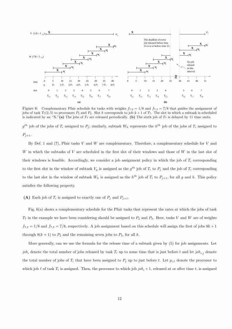
Figure 6: Complementary Pfair schedule for tasks with weights f7,2 = 1/8 and f7,3 = 7/8 that guides the assignment ofjobs of task T7(2, 5) to processors P2 and P3. Slot k corresponds to job k +1 of T7. The slot in which a subtask is scheduledis indicated by an “X.”(a) The jobs of T7 are released periodically. (b) The sixth job of T7 is delayed by 11 time units.
gth job of the jobs of Ti assigned to Pj ; similarly, subtask Wh represents the hth job of the jobs of Ti assigned to
Pj+1.
By Def. 1 and (7), Pfair tasks V and W are complementary. Therefore, a complementary schedule for V and
W in which the subtasks of V are scheduled in the first slot of their windows and those of W in the last slot of
their windows is feasible. Accordingly, we consider a job assignment policy in which the job of Ti corresponding
to the first slot in the window of subtask Vg is assigned as the gth job of Ti to Pj and the job of Ti corresponding
to the last slot in the window of subtask Wh is assigned as the hth job of Ti to Pj+1, for all g and h. This policy
satisfies the following property.
(A) Each job of Ti is assigned to exactly one of Pj and Pj+1.
Fig. 6(a) shows a complementary schedule for the Pfair tasks that represent the rates at which the jobs of task
T7 in the example we have been considering should be assigned to P2 and P3. Here, tasks V and W are of weights
f7,2 = 1/8 and f7,3 = 7/8, respectively. A job assignment based on this schedule will assign the first of jobs 8k + 1
through 8(k + 1) to P2 and the remaining seven jobs to P3, for all k.
More generally, can we use the formula for the release time of a subtask given by (5) for job assignments. Let
jobi denote the total number of jobs released by task Ti up to some time that is just before t and let jobi,j denote
the total number of jobs of Ti that have been assigned to Pj up to just before t. Let pi,` denote the processor to
which job ` of task Ti is assigned. Then, the processor to which job jobi + 1, released at or after time t, is assigned
12

is determined as follows.
pi,jobi+1 =
j, if jobi =⌊jobi,j
fi,j
⌋
j + 1, otherwise(8)
As before, let fi,j and fi,j+1 be the weights of two fictitious Pfair tasks V and W , respectively. Then, by (5),
tr =⌊jobi,j
fi,j
⌋denotes the release time of subtask Vjobi,j+1 of task V . Thus, (8) assigns to Pj , the job that
corresponds to the first slot in the window of subtask Vg as the gth job of Ti on Pj , for all g. (Recall that the index
of the job of the migrating periodic task Ti that is released in slot tr is given by tr + 1.) The job that corresponds
to the last slot in the window of subtask Wh is assigned as the hth job of Ti on Pj+1, for all h.
Thus far in our discussion, in order to simplify the exposition, we assumed that the job releases of task Ti are
periodic. However, note that the job assignment given by (8) is independent of “real” time and is based on the job
number only. Hence, assigning jobs using (8) should be sufficient to ensure (A) even when Ti is sporadic. This is
illustrated in Fig. 6(b). Here, we assume that T7 is a sporadic task, whose sixth job release is delayed by 11 time
units to time 36 from time 25. As far as T7 is concerned, the interval [25, 36) is “frozen” and the job assignment
resumes at time 36. As indicated in the figure, in any such interval in which activity is suspended for a migrating
task Ti, no jobs of Ti are released. Furthermore, the deadlines of all jobs of Ti released before the frozen interval
fall at or before the beginning of the interval.
We next prove a property that bounds from above the number of jobs of a migrating task assigned to each of
its processors by the job assignment rule given by (8).
Lemma 1 Let Ti be a migrating task that is assigned to processors Pj and Pj+1. The number of jobs out of any
consecutive ` ≥ 0 jobs of Ti that are assigned to Pj and Pj+1 is at most d` · fi,je and d` · fi,j+1e, respectively.
Proof: We prove the lemma for the number of jobs assigned to Pj . The proof for Pj+1 is similar. We first claim
the following.
(J) Exactly d`0 · fi,je of the first `0 jobs of Ti are assigned to Pj .
(J) holds trivially when `0 = 0. Therefore, assume `0 ≥ 1. Let q denote the total number of jobs of the first `0 jobs
of Ti that are assigned to Pj . (By (8), the first job of Ti is assigned to Pj , hence, q ≥ 1 holds.) Then, there exists
an `′ ≤ `0 such that job `′ of Ti is the qth job of Ti assigned to Pi. Therefore, by (8),
`′ − 1 =⌊
q − 1fi,j
⌋(9)
13
holds. `, `′, and q denote job numbers or counts, and hence are all non-negative integers. By (9), we have
q − 1fi,j
≥ `′ − 1 ⇒ q − 1 ≥ (`′ − 1) · fi,j ⇒ q ≥ `′ · fi,j {because fi,j < 1}, (10)
andq − 1fi,j
< `′ ⇒ q − 1 < `′ · fi,j ⇒ q < `′ · fi,j + 1. (11)
Because q is an integer, by (10) and (11), we have
q = d`′ · fi,je. (12)
If `′ = `0 holds, then (J) follows from (12) and our definition of q. On the other hand, to show that (J) holds when
`′ < `0, we must show that q = dˆ· fi,je holds for all ˆ, where `′ < ˆ ≤ `0. (Note that ˆ is an integer.) By the
definitions of q, `′, and `0, q of the first `′ jobs of Ti are assigned to Pj , and none of jobs `′ + 1 through `0 are
assigned to Pj . Therefore, by (8), it follows that ˆ− 1 <
⌊q
fi,j
⌋holds for all ˆ, where `′ < ˆ ≤ `0. Thus, we have
the following, for all ˆ, where `′ < ˆ ≤ `0.
⌊q
fi,j
⌋> ˆ−1 ⇒
⌊q
fi,j
⌋≥ ˆ ⇒ q
fi,j≥ ˆ ⇒ q ≥ ˆ·fi,j ⇒ q ≥ dˆ· fi,je {because q is an integer} (13)
By (12) and because ˆ> `′ holds, (13) implies that dˆ· fi,je = d`′ · fi,je = q holds.
Finally, we are left with showing that at most d` · fi,je of any consecutive ` jobs of Ti are assigned to Pj . Let
J represent jobs `0 + 1 to `0 + ` of Ti, where `0 ≥ 0. Then, by (J), exactly d`0 · fi,je of the first `0 jobs and
d(`0 + `) · fi,je of the first `0 + ` jobs of Ti are assigned to Pj . Therefore, the number of jobs belonging to J that
are assigned to Pj , denoted Jobs(J , j), is given by
Jobs(J , j) = d(`0 + `) · fi,je − d`0 · fi,je ≤ d`0 · fi,je+ d` · fi,je − d`0 · fi,je = d` · fi,je,
which proves the lemma. (The second step in the above derivation follows from dx + ye ≤ dxe+ dye.) ¥
We are now ready to derive a tardiness bound for EDF-fm.
3.3 Tardiness Bound for EDF-fm
As discussed earlier, jobs of migrating tasks do not miss their deadlines under EDF-fm. Also, if no migrating task
is assigned to processor Pk, then the fixed tasks on Pk do not miss their deadlines. Hence, our analysis is reduced
to determining the maximum amount by which a job of a fixed task may miss its deadline on each processor Pk,
14

in the presence of migrating jobs. We assume that two migrating tasks, denoted Ti and Tj , are assigned to Pk. (A
tardiness bound with only one migrating task can be derived from that obtained with two migrating tasks.) We
prove the following.
(L) The tardiness of every fixed task of Pk is at most ∆ = ei(fi,k+1)+ej(fj,k+1)1−si,k−sj,k
.
We prove (L) by contradiction. Contrary to (L), assume that job Tq,` of a fixed task Tq assigned to Pk has a
tardiness exceeding ∆. We use the following notation to assist with our analysis.
tddef= absolute deadline of job Tq,` (14)
tcdef= td + ∆ (15)
t0def= latest instance before tc that Pk was either idle or was executing a job of a fixed task
with a deadline later than td (16)
By our assumption that job Tq,` with absolute deadline at td has a tardiness exceeding ∆, it follows that Tq,` does
not complete execution at or before tc = td + ∆.
Let τk,f and τk,m denote the sets of all fixed and migrating tasks, respectively, that are assigned to Pk. (Note
that τk,m = {Ti, Tj}.) Let demand(τ, t0, tc) denote the maximum time that jobs of tasks in τ could execute in
the interval [t0, tc) on processor Pk (under the assumption that Tq,` does not complete executing at tc). We first
determine demand(τk,m, t0, tc) and demand(τk,f , t0, tc).
By (16) and because migrating tasks have higher priority than fixed tasks under EDF-fm, jobs of Ti and Tj
that are released before t0 and assigned to Pk complete executing at or before t0. Thus, every job of Ti or Tj that
executes in [t0, tc) on Pk is released in [t0, tc). Also, every job released in [t0, tc) and assigned to Pk places a demand
for execution in [t0, tc). The number of jobs of Ti that are released in [t0, tc) is at most⌈tc − t0
pi
⌉. By Lemma 1,
at most⌈fi,k
⌈tc − t0
pi
⌉⌉≤ fi,k
(tc−t0
pi+ 1
)+ 1 of all the jobs of Ti released in [t0, tc) are assigned to Pk. Similarly,
the number of jobs of Tj that are assigned to Pk of all jobs of Ti released in [t0, tc) is at most fj,k
(tc−t0
pj+ 1
)+ 1.
Each job of Ti executes for at most ei time units and that of Tj for ej time units. Therefore,
demand(τk,m, t0, tc) ≤(
fi,k
(tc − t0
pi+ 1
)+ 1
)· ei +
(fj,k
(tc − t0
pj+ 1
)+ 1
)· ej
= si,k(tc − t0) + ei(fi,k + 1) + sj,k(tc − t0) + ej(fj,k + 1) (17)
{by (2) and simplification}.
15
By (14)–(16), and our assumption that the tardiness of Tq,` exceeds ∆, any job of a fixed task that executes on
Pk in [t0, tc) is released at or after t0 and has a deadline at or before td. The number of such jobs of a fixed task
Tf is at most⌊td − t0
pf
⌋. Therefore,
demand(τk,f , t0, tc) ≤∑
Tf∈τk,f
⌊td − t0
pf
⌋· ef
≤ (td − t0)∑
Tf∈τk,f
ef
pf
≤ (td − t0)(1− si,k − sj,k) {by (P3)}. (18)
By (17) and (18), we have the following.
demand(τk,f ∪ τk,m, t0, tc) ≤ si,k(tc − t0) + ei(fi,k + 1) + sj,k(tc − t0) + ej(fj,k + 1) + (td − t0)(1− si,k − sj,k)
= (si,k + sj,k)(tc − td) + (si,k + sj,k)(td − t0) + ei(fi,k + 1)
+ej(fj,k + 1) + (td − t0)(1− si,k − sj,k)
= (si,k + sj,k)(tc − td) + ei(fi,k + 1) + ej(fj,k + 1) + (td − t0)
Because Tq,` does not complete executing by time tc, it follows that the total processor time available in the interval
[t0, tc] = tc − t0 < demand(τk,f ∪ τk,m, t0, tc), i.e.,
tc − t0 < (si,k + sj,k)(tc − td) + ei(fi,k + 1) + ej(fj,k + 1) + (td − t0)
⇒ tc − td < (si,k + sj,k)(tc − td) + ei(fi,k + 1) + ej(fj,k + 1)
⇒ tc − td <ei(fi,k + 1) + ej(fj,k + 1)
1− si,k − sj,k= ∆. (19)
The above contradicts (15), and hence our assumption that the tardiness of Tq,` exceeds ∆ is incorrect. Therefore,
(L) follows.
If only one migrating task Ti is assigned to Pk, then ej and sj,k are zero. Hence, a tardiness bound for any fixed
task on Pk is given byei(fi,k + 1)
1− si,k. (20)
If we let mk,`, where 1 ≤ ` ≤ 2 denote the indices of the migrating tasks assigned to Pk, then by (L), a tardiness
bound for EDF-fm is given by the following theorem.
Theorem 1 On M processors, Algorithm EDF-fm ensures a tardiness of at most
max1≤k≤M
emk,1(fmk,1,k + 1) + emk,2(fmk,2,k + 1)1− smk,1,k − smk,2,k
(21)
for every task set τ with Usum(τ) ≤ M and umax(τ) ≤ 1/2.
16
The tardiness bound given by Theorem 1 is directly proportional to the execution costs of the migrating tasks and
the shares assigned to them. This bound could be high if the share of each migrating task is close to 1/2. However,
because all tasks are light, in practice the sum of the shares of the migrating tasks assigned to a processor can be
expected to be less than 1/2. Theorem 1 also suggests that the tardiness that results in practice could be reduced
by choosing the set of migrating tasks carefully. Tardiness can also be reduced by distributing smaller pieces of
works of migrating tasks than entire jobs. Some such techniques are discussed in the next section.
4 Tardiness Reduction Techniques for EDF-fm
The problem of assigning tasks to processors such that the tardiness bound given by (21) is minimized is a combi-
natorial optimization problem with complexity that is exponential in the number of tasks. Hence, in this section,
we propose methods and heuristics that can lower tardiness. We consider the technique of period transformation [9]
as a way of distributing the execution of jobs of migrating tasks more evenly over their periods in order to reduce
the tardiness of fixed tasks. We also propose task assignment heuristics that can reduce the fraction of a processor’s
capacity consumed by migrating tasks.
Job-slicing approach. The tardiness bound of EDF-fm given by Theorem 1 is in multiples of the execution
costs of migrating tasks. This is a direct consequence of statically prioritizing migrating tasks over fixed tasks
and the overload (in terms of the number of jobs) that a migrating task may place on a processor over short
intervals. The deleterious effect of this approach on jobs of fixed tasks can be mitigated by “slicing” each job of a
migrating task into sub-jobs that have lower execution costs, assigning appropriate deadlines to the sub-jobs, and
distributing and scheduling sub-jobs in the place of whole jobs. For example, every job of a task with an execution
cost of 4 time units and relative deadline of 10 time units can be sliced into two sub-jobs with execution cost and
relative deadline of 2 and 5, respectively, per sub-job, or four sub-jobs with an execution cost of 1 and relative
deadline of 2.5, per sub-job. Such a job-slicing approach, termed period transformation, was proposed by Sha and
Goodman [9] in the context of RM scheduling on uniprocessors. Their purpose was to boost the priority of tasks
that have larger periods, but are more important than some other tasks with shorter periods, and thus ensure that
the more important tasks do not miss deadlines under overloads. However, with the job-slicing approach under
EDF-fm, it may be necessary to migrate a job between its processors, and EDF-fm loses the property that a task
that migrates does so only across job boundaries. Thus, this approach presents a trade-off between tardiness and
migration overhead.
Task-assignment heuristics. Another way of lowering the actual tardiness observed in practice would be to
lower the total share smk,1,k + smk,2,k assigned to the migrating tasks on any processor Pk. In the task assignment
algorithm Assign-Tasks of Fig. 1, if a low utilization-task is ordered between two high-utilization tasks, then it
is possible that smk,1,k + smk,2,k is arbitrarily close to one. For example, consider tasks Ti−1, Ti, and Ti+1 with
utilizations 1−ε2 , 2ε, and 1−ε
2 , respectively, and a task assignment wherein Ti−1 and Ti+1 are the migrating tasks
of Pk with shares of 1−2ε2 each, and Ti is the only fixed task on Pk. Such an assignment, which can delay Ti
excessively if the periods of Ti−1 and Ti+1 are large, can be easily avoided by ordering tasks by (monotonically)
decreasing utilization prior to the assignment phase. Note that with tasks ordered by decreasing utilization, of all
17

the tasks not yet assigned to processors, the one with the highest utilization is always chosen as the next migrating
task. Hence, we call this assignment scheme highest utilization first , or HUF. An alternative lowest utilization
first , or LUF, scheme can be defined that assigns fixed tasks in the order of (monotonically) decreasing utilization,
but chooses the task with the lowest utilization of all the unassigned tasks as the next migrating task. Such an
assignment can be accomplished using the following procedure when a migrating task needs to be chosen: traverse
the unassigned task array in reverse order starting from the task with the lowest utilization and choose the first task
whose utilization is at least the capacity available in the current processor. In general, this scheme can be expected
to lower the shares of migrating tasks. However, because the unassigned tasks have to be scanned each time a
migrating task is chosen, the time complexity of this scheme increases to O(NM) (from O(N)). This complexity
can be reduced to O(M log N) by adopting a binary search strategy.
A third task-assignment heuristic, called lowest execution-cost first , or LEF, that is similar to LUF, can be
defined by ordering tasks by execution costs, as opposed to utilizations. Fixed tasks are chosen in non-increasing
order of execution costs; the unassigned task with the lowest execution cost, whose utilization is at least that of
the available capacity in the current processor, is chosen as the next migrating task. The experiments reported in
the next section show that LEF actually performs the best of these three task-assignment heuristics and that when
combined with the job-slicing approach, can reduce tardiness dramatically in practice.
Including non-light tasks. The primary reason for restricting all tasks to be light is to prevent the total
utilization ui + uj of the two migrating tasks Ti and Tj assigned to a processor from exceeding one. (As already
noted, ensuring that migrating tasks do not miss their deadlines may not be possible otherwise.) However, if the
number of non-light tasks is small in comparison to the number of light tasks, then it may be possible to assign
tasks to processors without assigning two migrating tasks with total utilization exceeding one to the same processor.
In the simulation experiments discussed in Sec. 5, with no restrictions on per-task utilizations, the LUF approach
could successfully assign approximately 78% of the one million randomly-generated task sets on 4 processors. The
success ratio dropped to approximately one-half when the number of processors increased to 16.
Heuristic for processors with one migrating task. If the number of migrating tasks assigned to a processor
Pk is one, then the commencement of the execution of a job Ti,j of the only migrating task Ti of Pk can be postponed
to time d(Ti,j)−ei, where d(Ti,j) is the absolute deadline of job Ti,j (instead of beginning its execution immediately
upon its arrival). This would reduce the maximum tardiness of the fixed tasks on Pk to ei/(1 − si,k) (from the
value given by (20)). This technique will be particularly effective on two-processor systems, where each processor
would be assigned at most one migrating task only under EDF-fm, and on three-processor systems, where at most
one processor would be assigned two migrating tasks.
5 Experimental Evaluation
In this section, we describe the results of three sets of simulation experiments conducted using randomly-generated
task sets to evaluate EDF-fm and the heuristics described in Sec. 4.
The experiments in the first set evaluate the various task assignment heuristics for varying numbers of processors,
M , and varying maximum values of per-task utilization, umax. For each M and umax, 1, 000, 000 task sets were
18

0
50
100
150
200
250
300
350
400
15 20 25 30 35 40 45 50 55
Mea
n of
Max
imum
Tar
dine
ss
Maximum Execution Cost
Tardiness by Max. Execution Cost (M=8, u_max=0.5)
RandomHUFLUFLEF
LEF+Slicing
(a)
0
50
100
150
200
250
300
350
400
5 10 15 20 25
Mea
n of
Max
imum
Tar
dine
ss
Average Execution Cost
Tardiness by Avg. Execution Cost (M=8, u_max=0.5)
RandomHUFLUFLEF
LEF+Slicing
(b)
0
50
100
150
200
250
300
350
400
10 12 14 16 18 20 22 24 26
Mea
n of
Max
imum
Tar
dine
ss
Maximum Execution Cost
Tardiness by Max. Execution Cost (M=8, u_max=0.25)
RandomHUFLUFLEF
LEF+Slicing
(c)
0
50
100
150
200
250
300
350
400
4 5 6 7 8 9 10 11
Mea
n of
Max
imum
Tar
dine
ss
Average Execution Cost
Tardiness by Avg. Execution Cost (M=8, u_max=0.25)
RandomHUFLUFLEF
LEF+Slicing
(d)
0
50
100
150
200
250
300
350
400
0.25 0.3 0.35 0.4 0.45 0.5
Mea
n of
Max
imum
Tar
dine
ss
Maximum Utilization
Tardiness by Max. Utilization on 8 processors
RandomHUFLUFLEF
LEF+Slicing
(e)
0
50
100
150
200
250
300
350
400
0.1 0.15 0.2 0.25 0.3 0.35 0.4 0.45
Max
imum
Tar
dine
ss
Average Utilization
Tardiness by Utilization (Avg.) on 8 processors
RandomHUFLUFLEF
LEF+Slicing
(f)
Figure 7: Comparison of different task assignment heuristics. Tardiness for M = 8 and umax = 0.5 by (a) emax and (b)
eavg. Tardiness for M = 8 and umax = 0.25 by (c) emax and (d) eavg. Tardiness for M = 8 by (e) umax and (f) uavg.
generated. Each task set τ was generated as follows: New tasks were added to τ as long as the total utilization
of τ was less than M . For each new task Ti, first, its period pi was generated as a uniform random number in
the range [1, 100]; then, its execution cost was chosen randomly in the range [1/umax, umax · pi]. The last task was
generated such that the total utilization of τ exactly equaled M . The generated task sets were classified in four
different ways: (i) by the maximum execution cost of any task in a task set, emax, (ii) by the average execution
cost of a task set, eavg (iii) by the maximum utilization of any task in a task set, umax, and (iv) by the average
utilization of a task set, uavg. The tardiness bound given by (21) was computed for each task set under a random
task assignment and also under heuristics HUF, LUF, and LEF. The average value of the tardiness bound for task
sets in each group under each classification and heuristic was then computed. The results for the groups classified
by emax and eavg for M = 8 and umax = 0.5 are shown in insets (a) and (b), respectively, of Fig. 7. Insets (c) and
(d) contain the results under the same classifications for M = 8 and umax = 0.25. (99% confidence intervals are also
shown in these plots.) Results for classification by umax and uavg are given in insets (e) and (f), respectively. (It is
somewhat difficult to distinguish the plots in the figures. Mostly, the orders in the legend and the plots coincide.)
The plots show that LEF guarantees the minimum tardiness of the four task-assignment approaches. Tardiness
is quite low (approximately 8 time units mostly) under LEF for umax = 0.25 (insets (c), (d), and (e)), which
suggests that LEF may be a reasonable strategy for such task systems. Tardiness increases with increasing umax,
but is still a reasonable value of 25 time units only for eavg ≤ 10 when umax = 0.5. However, for eavg = 20,
tardiness exceeds 75 time units, which may not be acceptable. For such systems, tardiness can be reduced by using
19
0
20
40
60
80
100
2 4 6 8 10 12 14 16 18
% o
f tas
k se
ts a
ssig
ned
No. of processors (M)
Performance of LUF with non-light tasks
u_max=0.6u_max=0.7u_max=0.8u_max=0.9u_max=1.0
(a)
0
50
100
150
200
250
300
350
400
6 8 10 12 14 16 18 20 22 24
Mea
n of
Max
imum
Tar
dine
ss
Average Execution Cost
Estimated and Observed Tardiness under LEF
EstimatedObserved
(b)
0
50
100
150
200
250
300
350
400
0.2 0.25 0.3 0.35 0.4 0.45
Mea
n of
Max
imum
Tar
dine
ss
Average Utilization
Estimated and Observed Tardiness under LEF
EstimatedObserved
(c)
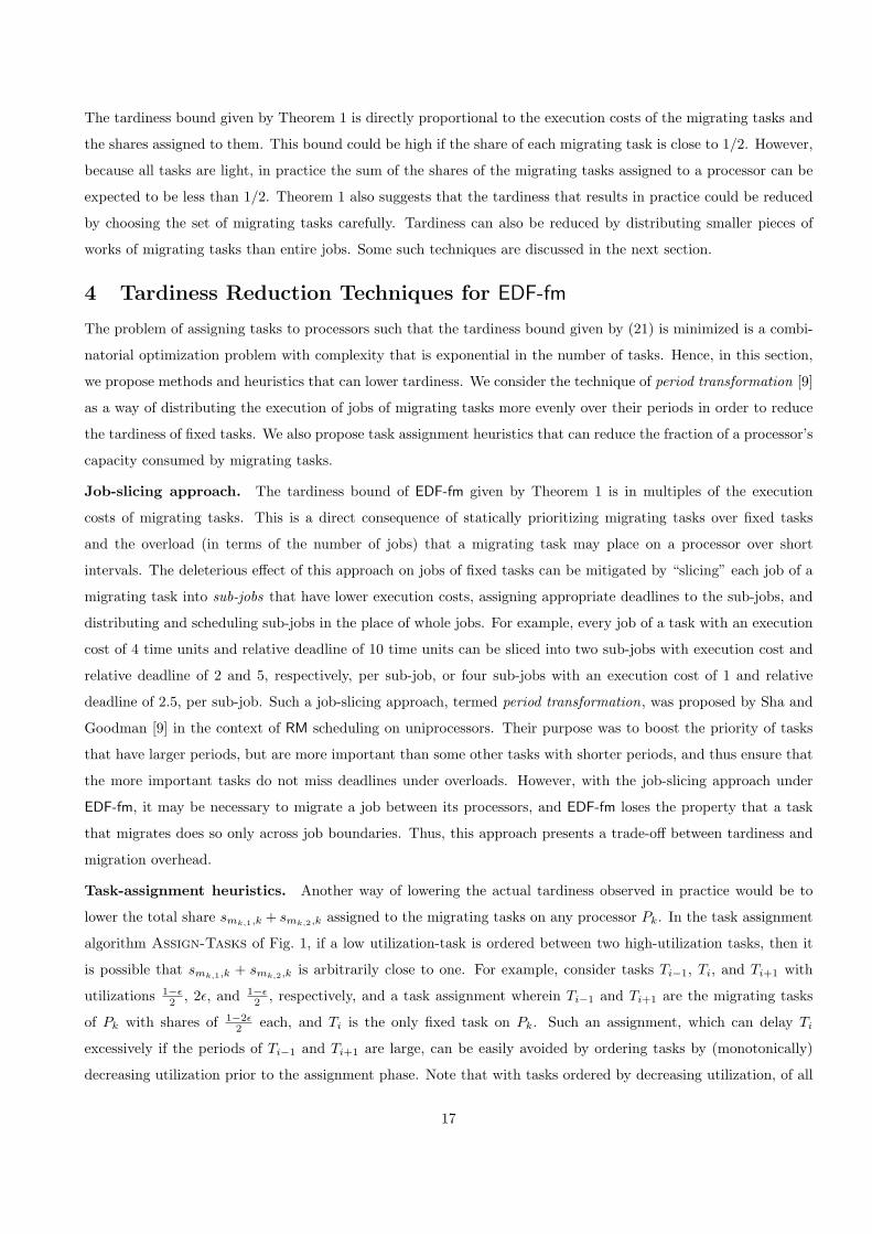
Figure 8: (a)Percentage of randomly-generated task sets with non-light tasks successfully assigned by the LUF heuristic.
(b) & (c) Comparison of estimated and observed tardiness under EDF-fm-LEF by (b) average execution cost and (c) average
utilization.
the job-slicing approach, at the cost of increased migration overhead. Therefore, in an attempt to determine the
reduction possible with the job-slicing approach, we also computed the tardiness bound under LEF assuming that
each job of a migrating task is sliced into sub-jobs with execution costs in the range [1, 2). This bound is also
plotted in the figures referred to above. For M > 4 and umax = 0.5, we found the bound to settle to approximately
7–8 time units, regardless of the execution costs and individual task utilizations. (When umax = 0.25, tardiness is
1–2 time units only under LEF with job slicing.) In our experiments, on average, a seven-fold decrease in tardiness
was observed with job slicing with a granularity of one to two time units per sub-job. However, a commensurate
increase in the number of migrations is also inevitable.
The second set of experiments evaluates the different heuristics in their ability to successfully assign task sets
that contain non-light tasks also. Task sets were generated using the same procedure as that described for the
first set of experiments above, except that umax was varied between 0.6 and 1.0 in steps of 0.1. All of the four
approaches could assign 100% of the task sets generated for M = 2, as expected. However, for higher values of M ,
the success ratio plummeted for all but the LUF approach. The percentage of task sets that LUF could successfully
assign for varying M and umax is shown in Fig. 8(a).
The third set of experiments was designed to evaluate the pessimism in the tardiness bound of (21). 300,000
task sets were generated with umax = 0.5 and Usum = 8. The tardiness bound estimated by (21) under the LEF
task assignment heuristic was computed for each task set. A schedule under EDF-fm-LEF for 100,000 time units was
also generated for each task set and the actual maximum tardiness observed was noted. (The time limit of 100,000
was determined by trial-and-error as an upper bound on the time within which tardiness converged for the tasks
sets generated.) Plots of the average of the estimated and observed values for tasks grouped by eavg and uavg are
shown in insets (b) and (c) of Fig. 8, respectively. In general, we found that actual tardiness is only approximately
half of the estimated value.
6 Concluding Remarks
We have proposed a new algorithm, EDF-fm, which is based on EDF, for scheduling recurrent soft real-time task
systems on multiprocessors, and have derived a tardiness bound that can be guaranteed under it. Our algorithm
20

places no restrictions on the total system utilization, but requires per-task utilizations to be at most one-half of a
processor’s capacity. This restriction is very liberal, and hence, our algorithm can be expected to be sufficient for
scheduling a large percentage of soft real-time applications. Furthermore, under EDF-fm, only a bounded number
of tasks need migrate, and each migrating task will execute on exactly two processors only. Thus, task migrations
are restricted and the migration overhead of EDF-fm is limited. We have also proposed the use of the job-slicing
technique, which can reduce the actual tardiness observed in practice, significantly.
Though a global EDF algorithm, with no restrictions on migration, would appear to be capable of guaranteeing
a lower tardiness bound than EDF-fm, we have so far not been able to derive a non-trivial bound under it. In fact,
we conjecture that a severe restriction on total utilization may be necessary, in addition to per-task utilization
restrictions, to guarantee a non-trivial tardiness bound under unrestricted EDF.
We have only taken a first step towards understanding tardiness under EDF-based algorithms on multiprocessors
and have not addressed all practical issues concerned. Foremost, the migration overhead of job slicing would
translate into inflated execution costs for migrating tasks, and to an eventual loss of schedulable utilization. Hence,
an iterative procedure for slicing jobs optimally may be essential. Next, our assumption that arbitrary task
assignments are possible may not be true if tasks are not independent. Therefore, given a system specification
that includes dependencies among tasks and tardiness that may be tolerated by the different tasks, a framework
that determines whether a task assignment that meets the system requirements is feasible, is required. Finally,
our algorithm, like every partitioning-based scheme, suffers from the drawback of not being capable of supporting
dynamic task systems in which the set of tasks and task parameters can change at runtime. We defer addressing
these issues to future work.
References
[1] T. P. Baker. Multiprocessor EDF and deadline monotonic schedulability analysis. In Proc. of the 24th IEEE Real-timeSystems Symposium, pages 120–129, Dec. 2003.
[2] S. Baruah and J. Carpenter. Multiprocessor fixed-priority scheduling with restricted interprocessor migrations. InProceedings of the 15th Euromicro Conference on Real-time Systems, pages 195–202. IEEE Computer Society Press, July2003.
[3] S. Baruah, N. Cohen, C.G. Plaxton, and D. Varvel. Proportionate progress: A notion of fairness in resource allocation.Algorithmica, 15:600–625, 1996.
[4] J. Carpenter, S. Funk, P. Holman, A. Srinivasan, J. Anderson, and S. Baruah. A categorization of real-time multiprocessorscheduling problems and algorithms. In Joseph Y. Leung, editor, Handbook on Scheduling Algorithms, Methods, andModels. Chapman Hall/CRC, 2004 (to appear).
[5] E. D. Jensen, C. D. Locke, and H. Tokuda. A time driven scheduling model for real-time operating systems. In Proc. ofthe 6th IEEE Real-time Systems Symposium, pages 112–122, 1985.
[6] C. Liu and J. Layland. Scheduling algorithms for multiprogramming in a hard real-time environment. Journal of theACM, 30:46–61, January 1973.
[7] J. Lopez, M. Garcia, J. Diaz, and D. Garcia. Worst-case utilization bound for edf scheduling on real-time multiprocessorsystems. In Proceedings of the 12th Euromicro Conference on Real-time Systems, pages 25–33, June 2000.
[8] A. Mok. Fundamental Design Problems of Distributed Systems for Hard Real-time Environments. PhD thesis, Massa-chusetts Institute of Technology, Cambridge, Mass., 1983.
[9] L. Sha and J. Goodenough. Real-time scheduling theory and Ada. IEEE Computer, 23(4):53–62, 1990.
21


![EDF-VD Scheduling of Mixed-Criticality Systems with ... · EDF-VD Scheduling of Mixed-Criticality Systems with Degraded Quality Guarantees Di Liu 1, ... [11]. In this paper, we ...](https://static.fdocuments.net/doc/165x107/5accae377f8b9ab10a8cbd8c/edf-vd-scheduling-of-mixed-criticality-systems-with-scheduling-of-mixed-criticality.jpg)