An economic production quantity inventory model with...

Scientia Iranica E (2016) 23(2), 736{746

Sharif University of TechnologyScientia Iranica

Transactions E: Industrial Engineeringwww.scientiairanica.com

An economic production quantity inventory model withbackorders considering the raw material costs

E.A. Pacheco-Vel�azqueza and L.E. C�ardenas-Barr�onb;�

a. Department of Industrial and Systems Engineering, Tecnol�ogico de Monterrey, Campus Ciudad de M�exico.b. School of Engineering and Sciences, Tecnol�ogico de Monterrey, E. Garza Sada 2501 Sur, C.P. 64849, Monterrey, Nuevo Le�on,

M�exico.

Received 1 October 2014; received in revised form 20 February 2015; accepted 4 May 2015

KEYWORDSEPQ;Inventory models;Raw materials;Manufacturingsystem.

Abstract. The classical Economic Production Quantity (EPQ) inventory model does notconsider ordering and holding costs of raw materials. In this direction, this paper considersthe ordering and holding costs for both raw materials and �nished product. Basically,four EPQ inventory models are developed from an easy perspective that has not beenconsidered before. It was found that the ordering and holding costs of raw materials mustbe taken into account, because they signi�cantly impact on the optimal production lot sizeof the �nished product in both EPQ without shortages and EPQ with shortages inventorymodels. Furthermore, an EPQ inventory model that determines the optimal lot size fora product that requires more than one raw material, and an EPQ inventory model thatobtains the optimal batch size for multiple products, which are manufactured with multipleraw materials, are proposed. Numerical examples are presented in order to illustrate theuse of the proposed inventory models.© 2016 Sharif University of Technology. All rights reserved.

1. Introduction

In recent years, a signi�cant progress has been made ininventory management. Management of the inventoriesis a mandatory activity that any company must do inthe best way. Therefore, the inventory has becomea key challenge for every production manager. It iswell known that the two classical inventory modelsof Economic Order Quantity (EOQ) and EconomicProduction Quantity (EPQ) have been proposed byHarris [1] and Taft [2], respectively. Afterwards, theconsultant, Wilson [3], made the EOQ popular, be-cause he applied it in practice in several companies. Itis important to remark that the EOQ inventory model

*. Corresponding author. Tel.: +52 81 83284235;Fax: +52 81 83284153E-mail addresses: [email protected] (E.A.Pacheco-Vel�azquez); [email protected] (L.E.C�ardenas-Barr�on)

determines the optimal order quantity to be purchased.Conversely, the EPQ inventory model calculates theoptimal production quantity to be manufactured. Sincethat the EOQ/EPQ inventory models appeared, manyresearchers and academicians have been constantlystudying and extending these inventory models in orderto model real life constraints. Two years ago, theEOQ inventory model celebrated its 100th anniversary.According to C�ardenas-Barr�on et al. [4], Ford WhitmanHarris is the Founding Father of Inventory Theory.

There is a vast literature on inventory modelsthat considers raw materials. For example, inventorymodels considering raw materials that satisfy the needsof a production process were proposed by Banerjee etal. [5], Golhar and Sarker [6], Jamal and Sarker [7],Sarker and Golhar [8], Sarker and Parija [9], Sarker etal. [10], Sarker and Parija [11], Sarker and Khan [12],Khan and Sarker [13], just to name a few works. Con-versely, there exists also a rich literature on inventorymodels for multiple products on one machine. Perhaps

Pacheco-Vel�azquez and C�ardenas-Barr�on/Scientia Iranica, Transactions E: Industrial Engineering 23 (2016) 736{746 737

Eilon [14] and Rogers [15] were the �rst researcherswho studied the multi products-single manufacturingsystem. Later, this type of the problem was treated ex-tensively in the works of Bomberger [16], Madigan [17],Stankard and Gupta [18], Hodgson [19], and Baker [20],just to name a few pioneer works that address multiproducts on a single machine. Later, Davis [21],Fransoo et al. [22], Sarker and Newton [23], Cooke etal. [24], and Hishamuddin et al. [25] continued studyingthis problem. The problem of multi products in onemachine is still being studied by several researchers.For example, Taleizadeh et al. [26] proposed an in-ventory model that considered multi products single-machine production system with stochastic scrappedproduction rate, partial backordering, and service levelconstraint. Their inventory model determined, foreach product, the optimal production quantity, theallowable shortage level, and the period length. Inthe same year, Taleizadeh et al. [27] developed anEPQ inventory model with backorders to determine theoptimal lot size and backorders level for multiproductmanufactured in a single machine. Also, Taleizadeh etal. [28] derived an EPQ inventory model with randomdefective items, service level constraints, and repairfailure. Basically, their inventory model obtained theoptimal cycle length, optimal lot size, and optimalbackordered level. Chiu et al. [29] obtained the optimalreplenishment lot size and shipment policy for an EPQinventory model with multiple deliveries and rework ofdefective products. Later, Taleizadeh et al. [30] solvedthe multiproduct single machine problem with andwithout rework considering backorders. Taleizadeh etal. [31] addressed the multi-product, multi-constraint,single period problem considering uncertain demandsand an incremental discount situation. On the otherhand, Sepehri [32] addressed a multi-period and multi-product problem in a multi-stage with multi-membersupply chain. Subsequently, Taleizadeh et al. [33] de-veloped an EPQ inventory model with rework processfor multi products in one machine and determined theoptimal cycle length as well as the optimal productionquantity for each product. In the same year, Rameza-nian and Saidi-Mehrabad [34] presented a Mixed Inte-ger Nonlinear Programming (MINLP) model to solvea multi-product unrelated parallel machines schedul-ing problem considering that the production systemcould manufacture imperfect products. Afterwards,Taleizadeh et al. [35] proposed an EPQ inventory modelwith random defective items and failure in repair formultiproduct in one machine environment. Later,Taleizadeh et al. [36] optimized a joint total cost foran imperfect, multi-product production system withrework subject to budget and service level constraints.In a subsequent paper, Taleizadeh et al. [37] devel-oped and analyzed an EPQ inventory model withinterruption in process, scrap, and rework. Their

inventory model considered multiple products and allproducts were processed in one machine. Recently,Holmbom et al. [38] developed a solution procedurethat solved the well-known Economic Lot SchedulingProblem (ELSP) when the machine had high utiliza-tion. Later, Holmbom and Segerstedt [39] gave ahistorical summary from Harris's [1] EOQ formulae tothe ELSP. Basically, they presented the complexitiesand di�culties in scheduling several products on onemachine subject to capacity constraint. Pal et al. [40]developed a stochastic inventory model that consideredtwo di�erent markets to sell the products: 1) for goodquality products, and 2) for average quality products.This inventory model also considers that the usedproducts' recovery rates from consumers are randomvariables and recovery products are put in storage intwo warehouses. After that, Roy et al. [41] proposed aneconomic production lot size model for a manufacturingsystem that produced defective products. The defec-tive products were accumulated and then reworked.This inventory model also permits shortages and thepartial and full backordering situations are analyzedand compared. Other relevant and related studies arethe research works of Hsu [42], Hsu and Hsu [43],Sana [44], Kumar et al. [45], Tripathi [46], Sana [47],Sana et al. [48], and Farughi et al. [49].

The rest of the paper is organized as follows. Sec-tion 2 introduces the problem and establishes the no-tation that is used through the whole paper. Section 3presents the mathematical formulation of the EPQ in-ventory model with raw material costs for multiple rawmaterials and one �nished product. Also, a comparisonwith the classical EPQ inventory model is made.Section 4 develops two EPQ inventory models. The�rst one is for multi-products without shortages withthe constraint that all products share the same setupcost for the production run. The second one is for thesituation when the products are comprised of multipleraw materials. Finally, Section 5 provides a conclusion.

2. Problem de�nition and notation

Regularly, the EPQ inventory model (see Figure 1)considers that at the beginning of the production run,there is not inventory cost due to the fact that there arenot �nished products. However, in the real world, thereare some costs that must be considered, because rawmaterials are procured with anticipation. Thus, theordering and holding costs of raw material are incurredbefore starting a production run. In this direction, thisresearch work has the main goal to include these costsin the development of the inventory models.

In any manufacturing process, at the beginningof every production run, it is necessary to prepare allthe raw materials required to complete lot size of the�nished products. This also means that an ordering

738 Pacheco-Vel�azquez and C�ardenas-Barr�on/Scientia Iranica, Transactions E: Industrial Engineering 23 (2016) 736{746

Figure 1. The classical inventory behavior in the EPQinventory model without shortages.

cost of the raw material is incurred when one placesan order on the supplier. Additionally, the holdingcost of raw material must be considered too. Thesecosts typically are ignored in the traditional EPQinventory model. Therefore, the cost of ordering theraw material and its holding cost must be consideredin the development of the inventory model.

Obviously, with the inclusion of the raw materialcosts, the optimal lot size of the �nished productwill change considerably. Consequently, in this paper,we propose an Economic Production Quantity (EPQ)without shortages and with shortages considering fullbackordering when the inventory of raw materials isinvolved.

The notations that will be used in this paper arede�ned and given below:D Demand rate (units/time unit);P Production rate (units/time unit);AP Setup cost of the production run

($/setup);hP Holding cost of the �nished product

($/unit/time unit);CP Production cost per �nished product

($/unit);AM Ordering cost of raw material

($/order);u Units required to produce one unit of

�nished product (units);hM Holding cost of raw material

($/unit/time unit);CM Raw material cost ($/unit);� Fixed backordering cost ($/unit);�t Linear backordering cost ($/unit/time

unit);Q� Production lot size (units);b� Backorders level (units);K Total cost.

Figure 2. Inventory behavior of (a) raw material withEOQ, and (b) �nished product with EPQ withoutshortages.

3. Development of the inventory models

3.1. An EPQ inventory model with rawmaterial costs and without shortages

First of all, it is necessary to develop an inventorymodel that considers the replenishment of raw materialand the manufacturing process, jointly. Basically, thismeans that the ordering and holding costs of rawmaterial must be included in the modelling of theinventory model (see Figure 2). It is assumed thatthe amount of raw materials ordered before must meetthe requirements for the production lot size within anyproduction cycle. Mathematically speaking, this canbe expressed as follows.

K(Q) =APDQ

+ hPQ2

�1� D

P

�+AM

DQ

+ uhMQ2DP: (1)

Algebraically, the above expression is reduced to:

K(Q)=(AP +AM )DQ

+Q2

�hP�

1�DP

�+uhM

DP

�:

(2)

In obtaining the global minimum optimal solution, thetotal cost function of the EPQ inventory model isoptimized via di�erential calculus. It is easy to seeand show that K(Q) is a convex function in Q. Then,by applying the optimization technique via di�erentialcalculus, one gets the optimal production lot size, givenby Eq. (3):

Q� =

s2(AP +AM )D

hP�1� D

P

�+ uhM D

P: (3)

It is obvious that if the ordering (AM ) and holding(hM ) costs of raw material are not considered, thenthe production lot size decreases immediately to theclassical EPQ without shortages.

3.2. An EPQ inventory model with rawmaterial costs and shortages

Now, this subsection presents an EPQ inventory modelwith raw material costs and shortages. Here, we


consider that the shortages occur only for the �nishedproduct. It is assumed that all shortages are backo-rdered. The total cost of the inventory model is givenbelow:

K(Q; b) = APDQ

+ hP

�Q�1� D

P

�� b�22Q�1� D

P

�+

�tb2

2Q�1� D

P

� +�bDQ

+AMDQ

+ uhMQ2DP: (4)

Thus:

K(Q; b) =(AP +AM )DQ

+ hP

�Q�1� D

P

�� b�22Q�1� D

P

�+

�tb2

2Q�1� D

P

� +�bDQ

+ uhMQ2DP: (5)

It is required to minimize the function K(Q; b) todetermine Q and b. It is easy to show that K(Q; b) is aconvex function in Q and b. Therefore, it is necessaryto di�erentiate K(Q; b), partially, with regard to Q andb. Hence, optimizing Eq. (5), one obtains the optimalproduction lot size and the optimal backorders level,which are given by Eqs. (6) and (7), respectively:

Q� =

s2(AP +AM )D(hP + �t)� �2D2

�1� D

P

�hP�t

�1� D

P

�+ hM uD

P (hP + �t);(6)

b� =(hPQ� �D)

�1� D

P

�hP + �t

: (7)

It is easy to see that the above expression for theproduction lot size immediately transforms into thewell-known equation of the EPQ with shortages when

both ordering (AM ) and holding (hM ) costs of rawmaterial are zero. In other words, it is when thesecosts are not considered.

3.3. Comparison with EPQ with and withoutshortages

In this section, a numerical comparison is made be-tween the results of the proposed inventory model andthose of the classical EPQ inventory model with andwithout shortages.

Numerical examples 1 and 2.The data for Examples 1 and 2 are given in the �rstcolumns of Tables 1 and 2, respectively. The resultsof the comparison with the EPQ without shortages arepresented in Table 1. In Table 2, they are given forthe comparison with the EPQ with shortages. In bothtables, we use the expression of w = uCM=CP . Thismeans that the raw material cost is a fraction of thecost of the �nished product. Typically, the holdingcosts are calculated as a percent of the cost (i.e., hP =iCP yhM = iCM ); then, the term w can be estimatedas w = uhM=hP .

Here, note that according to the results of Tables 1and 2, the optimal production lot size is sensible tothe fraction of cost of raw material in both inventorymodels. If the fraction increases, the production lotsize decreases.

3.4. An EPQ inventory model with multipleraw materials and one �nished product

It is now appropriate to discuss that in many situationsof the real life, a product is comprised of several rawmaterials. Although there is a unique �nished product,it is made of several raw materials; therefore, onecan apply the inventory models developed in the Sec-tions 3.1 and 3.2. There are always welcome practical

Table 1. Comparison of the proposed inventory model with EPQ without shortages.

AP hP AM w D P Q� Q� % ofdi�erenceEPQ Proposed inventory

50 2 20 0.1 500 1000 223.61 252.26 12.8250 2 20 0.3 500 1000 223.61 232.04 3.7750 2 20 0.5 500 1000 223.61 216.02 3.3950 2 20 0.7 500 1000 223.61 202.92 9.2550 2 20 0.9 500 1000 223.61 191.94 14.1

Table 2. Comparison of the proposed inventory model with EPQ with shortages.

AP hP AM w � �t D P Q� b� Q� b� Q bEPQ Proposed inventory % of di�erence

50 2 20 0.1 0.5 10 500 1000 238.48 9.45 268.72 11.98 12.68 26.7450 2 20 0.3 0.5 10 500 1000 238.48 9.45 243.86 9.90 2.25 4.8150 2 20 0.5 0.5 10 500 1000 238.48 9.45 224.83 8.32 5.73 11.9750 2 20 0.7 0.5 10 500 1000 238.48 9.45 209.65 7.05 12.09 25.3550 2 20 0.9 0.5 10 500 1000 238.48 9.45 197.19 6.02 17.32 36.34


perspectives in any company for applying mathemati-cal models. Therefore, in this direction, one needs justto establish the following oversimpli�cation, which issimple, easy to apply, and computationally e�cient.

Set AM1; AM2; � � � ; AMn as the ordering costs ofeach raw material; u1; u2; � � � ; un as the number ofunits of each raw material required to manufacture oneunit of the �nished product; and hM1; hM2; � � � ; hMn asthe holding cost of each raw material. Then, AM anduhM are de�ned as AM = AM1 +AM2 + � � �+AMn anduhM = u1hM1 +u2hM2 + � � �+unhMn, respectively. Asa result, one can use the previous proposed inventorymodels.

4. An EPQ inventory model without shortageswith multi-products and raw material costs

4.1. An EPQ inventory model withoutshortages with multi-products and oneraw material

Here, the situation is considered in which there isa unique raw material to process several �nishedproducts and these products are manufactured in onemachine or process. Consequently, it is assumed thatall products share one setup cost of the production run.In this type of problem, a schedule is required for thefabrication of products. A common cycle time is usedfor all the products. Figure 3 illustrates the commoncycle time.

It is easy to understand that in order to minimizethe holding cost of raw materials, it is necessary thatthe product with a higher consume rate of raw materialmust be scheduled �rst.

As an illustrative example, consider the situationof two products A and B. Suppose that one unit ofproduct A consumes 6 units of raw material and oneunit of product B requires 4 units of raw material.Moreover, the production rate of product A is 2000units per year and the production rate of product Bis 4000 units per year. Therefore, the consume ratesof raw material for products A and B are 12000 unitsper year and 16000 units per year, respectively. Asmentioned before, product B must be the �rst in theproduction schedule (i.e., the sequence is B-A).

Then the optimization problem can be expressedas:

minK(Q1; Q2; � � � ; Qn) = APDj

Qj

+nXk=1

�hk2Qk�

1� Dk

Pk

��+AM

Dj

Qj+ hM �I; (8)

subject to:

D1

Q1=D2

Q2= � � � = Dn

Qn; (9)

where �I represents the required units of raw materialand is given by Eq. (11). The details of the derivationof Eq. (11) are given in the Appendix.

Since:

Q2 =D2Q1

D1; Q3 =

D3Q1

D1; � � � ; Qn =

DnQ1

D1; (10)

and:

�I=Q1

2D1

8<: nXk=1

D2kukPk

+2n�1Xk=1

24Dk

Pk

0@ nXj=k+1

ujDj

1A359=; :(11)

Eq. (8) can be written as:

minK(Q1) = (AP +AM )D1

Q1

+Q1

2D1

(nXk=1

�hkDk

�1�Dk

Pk

��+

nXk=1

D2kukhMPk

+ 2n�1Xk=1

24Dk

Pk

0@ nXj=k+1

ujhMDj

1A35): (12)

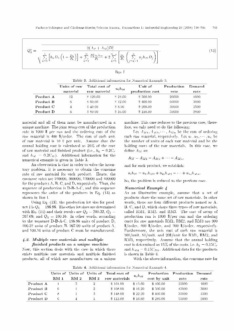
Optimizing Eq. (12), one can obtain the optimal lotsize for the product 1, which is given by Eq. (13) givenin Box I.

The optimal lot sizes for the rest of the productscan be easily calculated by the following equation:

Q�i =Di

D1Q�1: (14)

Numerical Example 3Consider a set of products that share the same raw

Figure 3. Inventory behavior of (a) raw material, (b) �nished product 1, and (3) �nished product 2 considering an EPQwithout shortages.


Q�1 =

vuuuut 2(AP +AM )D21

nPk=1

hhkDk

�1� Dk

Pk

�i+

nPk=1

D2kukhMPk + 2

n�1Pk=1

"DkPk

nP

j=k+1ujhMDj

!# : (13)

Box I

Table 3. Additional information for Numerical Example 3.

Units of rawmaterial

Total cost ofraw material

uihMUnit of

production costProduction

rateDemand

rateProduct A 12 $ 120.00 $ 24.00 $ 300.00 20000 4000Product B 6 $ 60.00 $ 12.00 $ 400.00 60000 3000Product C 4 $ 40.00 $ 8.00 $ 200.00 30000 1500Product D 8 $ 80.00 $ 16.00 $ 180.00 50000 2800

material and all of them must be manufactured in aunique machine. The joint setup cost of the productionrate is 1000 $ per run and the ordering cost of theraw material is 400 $/order. The cost of each unitof raw material is 10 $ per unit. Assume that theannual holding cost is calculated as 20% of the costof raw material and �nished product (i.e., hk = 0:2Ckand hM = 0:2CM ). Additional information for thenumerical example is given in Table 3.

An observation is that in order to solve the inven-tory problem, it is necessary to obtain the consumerate of raw material for each product. Hence, theconsume rates are 240000, 360000, 120000 and 400000for the products A, B, C, and D, respectively. Thus, thesequence of production is D-B-A-C, and this sequencerepresents the order of the products in Eq. (13) asshown in Box I.

Using Eq. (13), the production lot size for prod-uct 1 isQ1 = 186:96. The other lot sizes are determinedwith Eq. (14) and their results are Q2 = 200:32, Q3 =267:09, and Q4 = 100:16. In other words, accordingto the sequence D-B-A-C, 186.96 units of product D,200.32 units of product B, 267.09 units of product A,and 100.16 units of product C must be manufactured.

4.2. Multiple raw materials and multiple�nished products on a unique machine

Now, this section deals with the case in which thereexists multiple raw materials and multiple �nishedproducts, all of which are manufactures on a unique

machine. This case reduces to the previous case, there-fore, we only need to do the following:

Let AM1; AM2; � � � ; AMn be the cost of orderingeach raw material, respectively. Let u1; u2; � � � ; un bethe number of units of each raw material and be theholding costs of the raw materials. In this case, wede�ne AM as:

AM = AM1 +AM2 + � � �+AMn;

and for each product, we establish:

uihM = u1ihM1 + u2ihM2 + � � �+ unihMn:

So, the problem is reduced to the previous case.

Numerical Example 4As an illustrative example, assume that a set ofproducts share the same set of raw materials. In otherwords, there are four di�erent products named as A,B, C, and D, which share three types of raw materials,called RM1, RM2, and RM3. The cost of setup ofproduction run is 1000 $/per run and the orderingcosts for raw materials RM1, RM2, and RM3 are 300$/order, 400 $/order, and 200 $/order, respectively.Furthermore, the unit cost of each raw material is10$/unit, 8$/unit, and 20$/unit for RM1, RM2, andRM3, respectively. Assume that the annual holdingcost is determined as 15% of the costs, i.e. hk = 0:15Ckand hMk = 0:15CMk. Additional data for the productsis shown in Table 4.

With the above information, the consume rate for

Table 4. Additional information for Numerical Example 4.

Units ofRM 1

Units ofRM 2

Units ofRM 3

Total cost ofraw materials

uihMProductioncost by unit

Productionrate

Demandrate

Product A 4 3 2 $ 104.00 $ 15.60 $ 400.00 20000 4000Product B 6 1 2 $ 108.00 $ 16.20 $ 500.00 40000 3000Product C 8 1 3 $ 148.00 $ 22.20 $ 400.00 30000 1500Product D 6 4 1 $ 112.00 $ 16.80 $ 280.00 50000 2800


production of raw material, multiplied by uihM foreach product, is calculated. The values are: 312000,648000, 666000, and 840000 for products A, B, C, andD, respectively. Therefore, the schedule of productionis D-C-B-A. Thus, AM = AM1 + AM2 + AM3 = 900.Solving the problem, one obtains the lots sizes as Q1 =183:25, Q2 = 98:17, Q3 = 196:34, and Q4 = 261:79.In other words, according to the sequence D-C-B-A,183.25 units of product D, 98.17 units of product C,196.34 units of product B, and 261.79 units of productA must be manufactured in the machine.

5. Conclusion

In the traditional EPQ model, the ordering and holdingcosts of the raw material are not considered. Therefore,in this paper, a generalization of the EPQ inventorymodel of Taft (1918) was developed. The proposedinventory model considers both costs of raw material:ordering and holding. A main conclusion is that thesecosts must be taken into account, because they impact,directly, on the optimal production lot size. In bothinventory models, EPQ without shortages and EPQwith shortages were observed. It is concluded that theproduction lot size is very sensible to the costs of rawmaterial. The main new contribution of this paper ispresenting an EPQ inventory model that determinesthe optimal lot size for a product that requires morethan one raw material and an EPQ inventory modelthat determines the lot size for multiple products andmultiple raw materials.

Acknowledgments

The research for the second author was supported byTecnol�ogico de Monterrey Research Group in IndustrialEngineering and Numerical Methods 0822B01006. Theauthors would like to thank the three anonymousreferees for their valuable and helpful suggestions.These suggestions have strongly improved this paper.

References

1. Harris, F.W. \How many parts to make at once",Factory, The Magazine of Management, 10(2), pp.135-136, 152 (1913).

2. Taft, E.W. \The most economical production lot",Iron Age, 101, pp. 1410-1412 (1918).

3. Wilson, R.H. \A scienti�c routine for stock control",Harvard Business Review, 13, pp. 116-128 (1934).

4. C�ardenas-Barr�on, L.E., Chung, K.J. and Trevi~no-Garza, G. \Celebrating a century of the economic orderquantity model in honor of Ford Whitman Harris",International Journal of Production Economics, 155,pp. 1-7 (2014).

5. Banerjee, A., Sylla, C. and Eiamkanchanalai, S. \In-put/output lot sizing in single stage batch productionsystems under constant demand", Computers andIndustrial Engineering, 19(1-4), pp. 37-41 (1990).

6. Golhar, D.Y. and Sarker, B.R. \Economic manufac-turing quantity in a just-in-time delivery system",International Journal of Production Research, 30(5),pp. 961-972 (1992).

7. Jamal, A.M.M. and Sarker, B.R. \An optimal batchsize for a production system operating under a just-in-time delivery system", International Journal ofProduction Economics, 32(2), pp. 255-260 (1993).

8. Sarker, B.R. and Golhar, D.Y. \A reply to a note to\Economic manufacturing quantity in a just-in-timedelivery system"", International Journal of ProductionResearch, 31(11), p. 2749 (1993).

9. Sarker, B.R. and Parija, G.R. \An optimal batchsize for a production system operating under a �xed-quantity, periodic delivery policy", Journal of Opera-tional Research Society, 45(8), pp. 891-900 (1994).

10. Sarker, R.A., Karim, A.N.M. and Haque, A.F.M.A.\An optimal batch size for a production system operat-ing under a continuous supply/demand", InternationalJournal of Industrial Engineering, 2(3), pp. 189-198(1995).

11. Sarker, B.R. and Parija, G.R. \Optimal batch size andraw material ordering policy for a production systemwith a �xed-interval, lumpy demand delivery system",European Journal of Operational Research, 89(3), pp.593-608 (1996).

12. Sarker, R.A. and Khan, L.R. \An optimal batch sizefor a production system operating under periodic de-livery policy", Computers and Industrial Engineering,37(4), pp. 711-730 (1999).

13. Khan, L.R., Sarker, R.A. \An optimal batch size for aJIT manufacturing system", Computers and IndustrialEngineering, 42(2-4), pp. 127-136 (2002).

14. Eilon, S. \Scheduling for batch production", Journal ofInstitute of Production Engineering, 36, pp. 549-570,582 (1957).

15. Rogers, J. \A computational approach to the economiclot scheduling problem", Management Science, 4(3),pp. 264-291 (1958).

16. Bomberger, E.E. \A dynamic programming approachto a lot size scheduling problem", Management Sci-ence, 12(11), pp. 778-784 (1966).

17. Madigan, J.G. \Schedulling a multi-product singlemachine system for an in�nite planning period", Man-agement Science, 14(11), pp. 713-719 (1968).

18. Stankard, M.F. and Gupta, S.K. \A note onBomberger's approach to lot size scheduling: Heuristicproposed", Management Science, 15(7), pp. 449-452(1969).

19. Hodgson, T.J. \Addendum to standard and Gupta'snote on lot size scheduling", Management Science,16(7), pp. 514-517 (1970).


20. Baker, K.R. \On Madigan's approach to the de-terministic multi-product production and inventoryproblem", Management Science, 16(9), pp. 636-638(1970).

21. Davis, S.G. \Scheduling economic lot size produc-tion runs", Management Science, 36(8), pp. 985-998(1990).

22. Fransoo, J.C., Sridharan, V. and Bertrand, J.W.M. \Ahierarchical approach for capacity coordination in mul-tiple products single-machine production systems withstationary stochastic demands", European Journal ofOperational Research, 86(1), pp. 57-72 (1995).

23. Sarker, R.A. and Newton, C. \A genetic algorithmfor solving economic lot size scheduling problem",Computers and Industrial Engineering, 42(2-4), pp.189-198 (2002).

24. Cooke, D.L., Rohleder, T.R. and Silver, E.A. \Find-ing e�ective schedules for the economic lot schedul-ing problem: A simple mixed integer programmingapproach", International Journal of Production Re-search, 42(1), pp. 21-36 (2004).

25. Hishamuddin, H., Sarker, R.A. and Essam, D. \A dis-ruption recovery model for a single stage production-inventory system", European Journal of OperationalResearch, 222(3), pp. 464-473 (2012).

26. Taleizadeh, A.A., Wee, H.M. and Sadjadi, S.J. \Multi-product production quantity model with repair failureand partial backordering", Computers and IndustrialEngineering, 59(1), pp. 45-54 (2010a).

27. Taleizadeh, A.A., Naja�, A.A. and Niaki, S.T.A. \Eco-nomic production quantity model with scrapped itemsand limited production capacity", Scientia Iranica E,17(1), pp. 58-69 (2010).

28. Taleizadeh, A.A., Niaki, S.T.A. and Naja�, A.A.\Multiproduct single-machine production system withstochastic scrapped production rate, partial backorder-ing and service level constraint", Journal of Compu-tational and Applied Mathematics, 233(8), pp. 1834-1849 (2010).

29. Chiu, S.W., Lin, H.-D., Wu, M.-F. and Yang, J.-Ch. \Determining replenishment lot size and shipmentpolicy for an extended EPQ model with delivery andquality assurance issues", Scientia Iranica E, 18(6),pp. 1537-1544 (2011).

30. Taleizadeh, A.A., Sadjadi, S.J. and Niaki, S.T.A.\Multiproduct EPQ model with single machine, back-ordering and immediate rework process", EuropeanJournal of Industrial Engineering, 5(4), pp. 388-411(2011a).

31. Taleizadeh, A.A., Shavandi, H. and Haji, R. \Con-strained single period problem under demand un-certainty", Scientia Iranica E, 18(6), pp. 1553-1563(2011b).

32. Sepehri, M. \Cost and inventory bene�ts of coop-eration in multi-period and multi-product supply",Scientia Iranica E, 18(3), pp. 731-741 (2011).

33. Taleizadeh, A.A., C�ardenas-Barr�on, L.E., Biabani, J.and Nikousokhan, R. \Multi products single machineEPQ model with immediate rework process", Inter-national Journal of Industrial Engineering Computa-tions, 3(2), pp. 93-102 (2012).

34. Ramezanian, R. and Saidi-Mehrabad, M. \Multi-product unrelated parallel machines scheduling prob-lem with rework processes", Scientia Iranica E, 19(6),pp. 1887-1893 (2012).

35. Taleizadeh, A.A., Wee, H.M. and Jalali-Naini, S.G.\Economic production quantity model with repairfailure and limited capacity", Applied MathematicalModelling, 37(5), pp. 2765-2774 (2013).

36. Taleizadeh, A.A., Jalali-Naini, S.G., Wee, H.M. andKuo, T.C. \An imperfect multi-product productionsystem with rework", Scientia Iranica E, 20(3), pp.811-823 (2013).

37. Taleizadeh, A.A., C�ardenas-Barr�on, L.E. and Mo-hammadi, B. \A deterministic multi product singlemachine EPQ model with backordering, scraped prod-ucts, rework and interruption in manufacturing pro-cess", International Journal of Production Economics,150(1), pp. 9-27 (2014).

38. Holmbom, M., Segerstedt, A. and Sluis, E. \A solutionprocedure for economic lot scheduling problems evenin high utilization facilities", International Journal ofProduction Research, 51(12), pp. 3765-3777 (2013).

39. Holmbom, M. and Segerstedt, A. \Economic orderquantities in production: From Harris to economiclot scheduling problems", International Journal ofProduction Economics, 155, pp. 82-90 (2014).

40. Pal, B., Sana, S.S. and Chaudhuri, K. \A stochastic in-ventory model with product recovery", CIRP Journalof Manufacturing Science and Technology, 6(2), pp.120-127 (2013).

41. Roy, M.D., Sana, S.S. and Chaudhuri, K. \An eco-nomic production lot size model for defective itemswith stochastic demand, backlogging and rework",IMA Journal of Management Mathematics, 25(2), pp.159-183 (2014).

42. Hsu, L.F. \A note on \An Economic Order Quantity(EOQ) for items with imperfect quality and inspectionerrors"", International Journal of Industrial Engineer-ing Computations, 3(4), pp. 695-702 (2012).

43. Hsu, J.T. and Hsu, L.F. \An integrated single-vendor single-buyer production-inventory model foritems with imperfect quality and inspection errors",International Journal of Industrial Engineering Com-putations, 3(5), pp. 703-720 (2012).

44. Sana, S.S. \A collaborating inventory model in asupply chain", Economic Modelling, 29(5), pp. 2016-2023 (2012).

45. Kumar, N., Singh, S.R. and Kumari, R. \Two-warehouse inventory model of deteriorating items withthree-component demand rate and time-proportionalbacklogging rate in fuzzy environment", InternationalJournal of Industrial Engineering Computations, 4(4),pp. 587-598 (2013).


46. Tripathi, R.P. \Inventory model with di�erent demandrate and di�erent holding cost", International Journalof Industrial Engineering Computations, 4(3), pp. 437-446 (2013).

47. Sana, S.S. \Optimal production lot size and reorderpoint of a two-stage supply chain while random de-mand is sensitive with sales teams' initiatives", Inter-national Journal of Systems Science, 47(2), pp. 450-465 (2016).

48. Sana, S.S., Chedid, J.A. and Salas Navarro, K. \Athree layer supply chain model with multiple suppli-ers, manufacturers and retailers for multiple items",Applied Mathematics and Computation, 229, pp. 139-150 (2014).

49. Farughi, H., Khanlarzade, N. and Yegane, B.Y. \Pric-ing and inventory control policy for non-instantaneousdeteriorating items with time- and price-dependentdemand and partial backlogging", Decision ScienceLetters, 3(3), pp. 325-334 (2014).

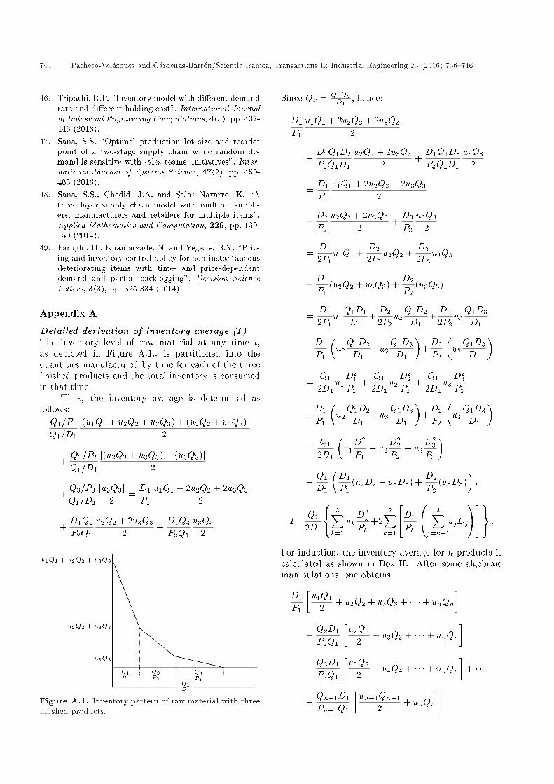
Appendix A

Detailed derivation of inventory average (�I)The inventory level of raw material at any time t,as depicted in Figure A.1., is partitioned into thequantities manufactured by time for each of the three�nished products and the total inventory is consumedin that time.

Thus, the inventory average is determined asfollows:Q1=P1

Q1=D1

[(u1Q1 + u2Q2 + u3Q3) + (u2Q2 + u3Q3)]2

+Q2=P2

Q1=D1

[(u2Q2 + u3Q3) + (u3Q3)]2

+Q3=P3

Q1=D1

[u3Q3]2

=D1

P1

u1Q1 + 2u2Q2 + 2u3Q3

2

+D1Q2

P2Q1

u2Q2 + 2u3Q3

2+D1Q3

P3Q1

u3Q3

2:

Figure A.1. Inventory pattern of raw material with three�nished products.

Since Qk = Q1DkD1

, hence:

D1

P1

u1Q1 + 2u2Q2 + 2u3Q3

2

+D1Q1D2

P2Q1D1

u2Q2 + 2u3Q3

2+D1Q1D3

P3Q1D1

u3Q3

2

=D1

P1

u1Q1 + 2u2Q2 + 2u3Q3

2

+D2

P2

u2Q2 + 2u3Q3

2+D3

P3

u3Q3

2

=D1

2P1u1Q1 +

D2

2P2u2Q2 +

D3

2P3u3Q3

+D1

P1(u2Q2 + u3Q3) +

D2

P2(u3Q3)

=D1

2P1u1Q1D1

D1+D2

2P2u2Q1D2

D1+D3

2P3u3Q1D3

D1

+D1

P1

�u2Q1D2

D1+u3

Q1D3

D1

�+D2

P2

�u3Q1D3

D1

�=

Q1

2D1u1D2

1P1

+Q1

2D1u2D2

2P2

+Q1

2D1u3D2

3P3

+D1

P1

�u2Q1D2

D1+u3

Q1D3

D1

�+D2

P2

�u3Q1D3

D1

�=

Q1

2D1

�u1D2

1P1

+ u2D2

2P2

+ u3D2

3P3

�+Q1

D1

�D1

P1(u2D2 + u3D3) +

D2

P2(u3D3)

�;

�I=Q1

2D1

8<: 3Xk=1

ukD2k

Pk+2

2Xk=1

24Dk

Pk

0@ 3Xj=k+1

ujDj

1A359=; :

For induction, the inventory average for n products iscalculated as shown in Box II. After some algebraicmanipulations, one obtains:

D1

P1

�u1Q1

2+ u2Q2 + u3Q3 + � � �+ unQn

�+Q2D1

P2Q1

�u2Q2

2+ u3Q3 + � � �+ unQn

�+Q3D1

P3Q1

�u3Q3

2+ u4Q4 + � � �+ unQn

�+ � � �

+Qn�1D1

Pn�1Q1

�un�1Qn�1

2+ unQn

�


Q1=P1

Q1=D1

[(u1Q1 + u2Q2 + u3Q3 + � � �+ unQn) + (u2Q2 + u3Q3 + � � �+ unQn)]2

+Q2=P2

Q1=D1

[(u2Q2 + u3Q3 + � � �+ unQn) + (u3Q3 + � � �+ unQn)]2

+Q3=P3

Q1=D1

[(u3Q3 + � � �+ unQn) + (u4Q4 + � � �+ unQn)]2

+ � � �

+Qn�1=Pn�1

Q1=D1

[un�1Qn�1 + unQn + unQn]2

+Qn=PnQ1=D1

unQn2

:

Box II

+QnD1

PnQ1

�unQn

2

�:

Since that D1Q1

= D2Q2

= � � � = DnQn , thus Qk = DkQ1

D1.

Therefore, by substituting Qk, we have:

D1

P1

�u1Q1

2+ u2Q2 + u3Q3 + � � �+ unQn

�+D2Q1D1

P2Q1D1

�u2Q2

2+ u3Q3 + � � �+ unQn

�+D3Q1D1

P3Q1D1

�u3Q3

2+ u4Q4 + � � �+ unQn

�+Dn�1Q1D1

Pn�1Q1D1

�un�1Qn�1

2+ unQn

�+DnQ1D1

PnQ1D1

�unQn

2

�:

Simplifying:

D1

P1

�u1Q1

2+ u2Q2 + u3Q3 + � � �+ unQn

�+D2

P2

�u2Q2

2+ u3Q3 + � � �+ unQn

�+D3

P3

�u3Q3

2+ u4Q4 + � � �+ unQn

�+Dn�1

Pn�1

�un�1Qn�1

2+ unQn

�+Dn

Pn

�unQn

2

�;

after some algebraic manipulations:�D1

P1

u1Q1

2+D2

P2

u2Q2

2+D3

P3

u3Q3

2+� � �+Dn

PnunQn

2

�+D1

P1[u2Q2 + u3Q3 + � � �+ unQn]

+D2

P2[u3Q3 + � � �+ unQn] + � � �

+Dn�1

Pn�1[unQn];

the �rst part can be expressed as:

D1

P1

u1Q1

2+D2

P2

u2Q2

2+D3

P3

u3Q3

2+ � � �

+Dn

PnunQn

2=

nXk=1

DkukQk2Pk

:

Substituting the expression of Qk:

nXk=1

DkukQk2Pk

=nXk=1

D2kukQ1

2D1Pk=

Q1

2D1

nXk=1

D2kukPk

;

the second part can be expressed as:

D1

P1[u2Q2 + u3Q3 + � � �+ unQn]

+D2

P2[u3Q3 + � � �+ unQn] + � � �

+Dn�1

Pn�1[unQn]

=n�1Xk=1

24Dk

Pk

0@ nXj=k+1

ujQj

1A35=n�1Xk=1

24Dk

Pk

0@ nXj=k+1

ujQ1Dj

D1

1A35=Q1

D1

n�1Xk=1

24Dk

Pk

0@ nXj=k+1

ujDj

1A35


= 2Q1

2D1

n�1Xk=1

24Dk

Pk

0@ nXj=k+1

ujDj

1A35 :Thus, the inventory average is given by:

�I =Q1

2D1

(nXk=1

D2kukPk

+2n�1Xk=1

24Dk

Pk

0@ nXj=k+1

ujDj

1A359=; :

Biographies

Ernesto Armando Pacheco-Vel�azquez is currentlya Professor in the Department of Industrial and Sys-tems Engineering at Tecnol�ogico de Monterrey, Cam-pus Ciudad de M�exico, M�exico. He has been teachingand researching at Tecnol�ogico de Monterrey for more

than 25 years. He has published several papers. Hisresearch areas primarily include inventory, logistics,supply chain, decision making, and voting.

Leopoldo Eduardo C�ardenas-Barr�on is currentlya Professor at the School of Engineering and Sciences atTecnol�ogico de Monterrey, Campus Monterrey, M�exico.He is also a faculty member in the Department ofIndustrial and Systems Engineering at Tecnol�ogico deMonterrey. He was the associate director of the Indus-trial and Systems Engineering programme from 1999to 2005. Moreover, he was the associate director ofthe Department of Industrial and Systems Engineeringfrom 2005 to 2009. His research areas primarily includeinventory planning and control, logistics, and supplychain. He has published papers and technical notesin several national and international journals. He hasco-authored one book in the �eld of Simulation inSpanish. He is also editorial board member in severalinternational journals.

An economic production quantity inventory model with...

Documents

Transcript of An economic production quantity inventory model with...