An Econometric Model of International Growth Dynamics for Long-horizon

Forecasting

June 3, 2020

Ulrich K. Müller Department of Economics, Princeton University

James H. Stock

Department of Economics, Harvard University and the National Bureau of Economic Research

and

Mark W. Watson*

Department of Economics and the Woodrow Wilson School, Princeton University and the National Bureau of Economic Research

* For helpful comments we thank participants at several seminars and in particular those at the Resources for the Future workshop on Long-Run Projections of Economic Growth and Discounting. Müller acknowledges financial support from the National Science Foundation grant SES-1919336. An earlier version of this paper used the title "An Econometric Model of International Growth Dynamics."

Abstract

We develop a Bayesian latent factor model of the joint long-run evolution of GDP per capita for

113 countries over the 118 years from 1900 to 2017. We find considerable heterogeneity in rates

of convergence, including rates for some countries that are so slow that they might not converge

(or diverge) in century-long samples, and a sparse correlation pattern (“convergence clubs”)

between countries. The joint Bayesian structure allows us to compute a joint predictive

distribution for the output paths of these countries over the next 100 years. This predictive

distribution can be used for simulations requiring projections into the deep future, such as

estimating the costs of climate change. The model’s pooling of information across countries

results in tighter prediction intervals than are achieved using univariate information sets. Still,

even using more than a century of data on many countries, the 100-year growth paths exhibit

very wide uncertainty.

Key words: Long-horizon forecasts, growth convergence, Social Cost of Carbon, global growth JEL: O47, C32, C55

1

1. Introduction

Long-run planning, policy evaluation, and pricing of long-lived assets requires long-

horizon forecasts. Issues involved in climate change provide leading examples. For example,

among the many technical problems in the economics of climate change is the need to make

projections of global and regional economic growth into the deep future. Future levels of GDP

drive future energy consumption, future emissions of carbon dioxide, the economic capacity to

reduce those emissions, and human ability to adapt to the changing climate caused by those

emissions. This paper develops a probability model of the joint growth of national per-capita

GDP, estimated using up to 118 years of data on 113 countries. The premise of this exercise is

that the joint stochastic process followed by the long-run growth of national incomes over the

past century is a useful starting point for projecting their evolution – more precisely, for

computing their joint predictive probability distribution – over the next 100 years. The resulting

joint predictive distribution can be used to gauge uncertainty about future long-run growth in

individual countries or groupings of countries by region or stage of development.1 The advantage

of such a joint modelling approach over country specific individual forecasts is not only that one

obtains a coherent joint prediction, but it also enables cross-country learning about key growth

characteristics and incorporates useful cross-country constraints. 2

The analysis builds on the long-horizon prediction methods developed in Müller and

Watson (2016), but extends that univariate analysis to a large 113-country multivariate

framework. We posit a long-run parametric model of international growth dynamics that is

informed by the vast empirical literature on international growth, development and

convergence.3 In particular, the model incorporates five features that the previous literature

suggests characterize long-term economic growth. First, the model contains a single global factor

to which countries converge in expectation, although the rate of this convergence is allowed to

1 The original motivation for this work was the development of long-run probabilistic forecasts of global and regional growth for use in estimating the Social Cost of Carbon, which is the monetized net present value of the economic damages resulting from emitting an additional ton of carbon dioxide. See National Academy of Sciences (2017, Ch. 3) for discussion. 2 We compare the forecasts from our joint model with univariate forecasts from individual countries in Section 6.4 and find, for example, that the median univariate forecast for GDP per capita in South Korea in 2118 is 6 times higher than in the U.S. due to an unconstrained extrapolation of higher in-sample growth. 3 Classic references include Barro (1991) and Mankiw, Romer and Weil (1992). See Jones (2016) and Johnson and Papageorgiou (2020) for recent reviews.

2

be heterogeneous across countries. Second, if these rates of convergence to the global factor are

sufficiently slow, a century-long realization can produce apparent convergence to parallel paths

(so-called conditional convergence). Third, an individual country can have a highly variable

long-term growth rate, including strong multidecadal growth and prolonged periods of economic

collapse. Fourth, the model allows for “convergence clubs,” that is, clusters of countries with

highly correlated long-run income levels within the cluster. Fifth, the global factor itself is

allowed to evolve in a flexible way that, consistent with the historical evidence, allows for

persistent changes in its underlying mean growth rate. We build these features into a multi-factor

Bayesian dynamic factor model, where the factors are distinguished by their dynamics and their

(latent) commonality across groups of countries.

The focus on long-run dynamics and long-horizon forecasts leads to several

simplifications in modeling and estimation. First, it allows us to abstract from short-run and

business-cycle factors by filtering the data to eliminate variation associated with periods shorter

than 15 years. With this shorter-run variation eliminated, the model needs only to focus on the

longer-run dynamics relevant for long-horizon forecasts. Second, the low-frequency filtering is

implemented using weighted averages of the raw data; these low-frequency averages are

approximately normally distributed even when the raw data are non-normal and/or highly

persistent. This allows us to specify a Gaussian probability model for estimation and forecasting,

despite the non-normal characteristics of the underlying data.

We begin in Section 2 with a description of the data, which is a panel of GDP per capita

for 113 countries from 1900 to 2017, taken from the Penn World Table (Feenstra, Inklarr and

Timmer (2015)) and the updated Maddison Project Database (Bolt, Inklarr, de Jong and van

Zanden (2018)). The panel data set is unbalanced, with missing data for some countries in some

years. Plots and descriptive statistics highlight five features of the data, echoing previous

findings in the growth literature: a common growth factor, persistent changes in long-term

growth rates within countries, a temporally stable dispersion of the historical cross-sectional

distribution, extremely persistent country-specific effects, and a possible group structure of

cross-country correlations.

Section 3 outlines an econometric model that captures these features. The model has a

simple structure, but it allows cross-country heterogeneity and a flexible pattern of dynamic

3

covariability across the 113 countries. This flexibility comes at the expense of introducing

hundreds of unknown parameters.

Section 4 takes up the problem of estimating these parameters and computing the long-

horizon joint predictive distribution for the 113 countries. We focus on 50- and 100-year ahead

predictions. Bayes estimation of a high dimensional model (n = 113 countries, T = 118 years and

over unknown 800 parameters) with missing data, and with a goal of estimating a joint predictive

distribution 100 years into the future, presents considerable computational challenges. As we

show, however, the structure of the model, priors, and data transformations yield important

simplifications. Because the long-run nature of our analysis allows us to focus on low-frequency

averages of the raw data, the effective dimension of the data is reduced by a factor of

approximately seven. And, because those low-frequency averages follow normal laws in large-

samples, estimation can be based on a Gaussian likelihood and predictive distributions can be

deduced from familiar Gaussian formulae. The model incorporates a linear factor structure,

which facilitates missing data and the use of Gibbs MCMC methods. These features, together

with the structure of the priors introduced in Section 4, makes Bayes estimation feasible; indeed,

we computed all the results for our benchmark model in a matter of minutes using a 24-core

workstation.

Section 5 summarizes results for the historical period for which we have data. These

results complement and generalize those found in the empirical growth and convergence

literature.

Section 6 presents our main results, which are long-horizon (50- and 100-year ahead)

joint-predictive distributions for the 113 countries. Results are presented for a baseline

specification and several alternatives, including a set of 113 country-specific univariate models.

The section also summarizes two external validity exercises: a pseudo-out-of-sample forecasting

experiment and an application of the model to long-horizon forecasting for average labor

productivity (GDP per worker).

Concluding remarks are offered in Section 7.

2. Data and Descriptive Statistics

2.1 The data

4

The data are annual values of real per-capita GDP for 113 countries spanning the 118-

year period 1900-2017, taken from the Penn Word Table (Feenstra, et. al. (2015)) and Bolt et.

al.’s (2018) Maddison Project Database. GDP is measured at constant 2011 national prices,

expressed in U.S. dollars.4

The 113 countries are those with at least 50 years of available data and 2017 population

levels of at least 3 million people. The resulting 113 countries account for 96% of world GDP

and 97% of world population in 2017. Of the 69 countries in the Penn World Table that are

excluded, 41 are excluded because of limited data (the largest being Ukraine, which has only 38

years of data), 54 because of a small population (the average 2017 population is less than one

million for these countries), and 26 for both reasons. The 113 included countries are depicted in

Figure 1. The data set is an unbalanced panel with between 36 and 52 countries for the years

1900-1949, 108 countries in 1950, 111 in 1952, and all 113 beginning in 1960. Appendix 1

discusses the data in more detail and lists the countries and sample periods.

The data, in logarithms, are plotted in Figure 2.

2.2 Long-run components

The paths of GDP per capita in Figure 2 exhibit both long-run movements and high

frequency fluctuations arising from measurement error, business cycles, and other relatively

short-lived sources. Because our interest is in modeling the long-run growth properties of these

data, we adopt a procedure that eliminates short-run fluctuations while retaining long-run trends.

In principle, trend extraction can be done using a low-pass filter. The specific method we

use is from Müller and Watson (2008, 2018) and reviewed in Müller and Watson (2019). For a

given time series yt, the low-frequency trend is the fitted value from the OLS regression of yt

onto a vector Xt which consists of a linear trend, a constant, and q-1 low-frequency periodic

functions.5

4 Specifically, real GDP is rgdpna from the Penn World Table and population is population. We link these series to per-capita GDP rgdpnapc and pop from the Maddison database beginning in the earliest available Penn World Table date for each country (typically 1950). 5 Müller and Watson (2018) use a constant term and Type II cosine transforms for the periodic regressors to compute the low-frequency trend. Here we also include a linear time trend and, following Müller and Watson (2008), use the q-1 eigenvectors of the covariance matrix of a detrended random walk for the periodic regressors associated with the largest eigenvalues.

ˆty

5

This low-frequency trend extraction method has three useful features. First, as shown in

Müller and Watson (2008), it well-approximates an ideal “low-pass” filter that extracts

periodicities longer than 2T/q, where T is the sample size and q is the number of regressors

excluding the constant term. We focus on periodicities longer than 14 years, so for countries with

a full set of T =118 years of data we use q =16 ≈ 2×118/14. Second, as shown in Müller and

Watson (2008, 2019), under quite general conditions on the stochastic process for yt (including

unit root and fractionally integrated models), the OLS regression coefficients are approximately

jointly normal. Thus inference and Bayesian modeling can treat the trend coefficients as

Gaussian even if the underlying data are not. Third, this method is in effect a data compression

method that reduces the dimensionality of the data from T to q+1, which provides considerable

computational advantages.

The method is illustrated in Figure 3. Panel (a) focuses on countries with data available

over the entire 1900-2017 sample period. The first panel plots the regressors Xt: the linear trend,

the constant, and the periodic functions. The remaining panels show the logarithm of GDP per

capita for various countries (yi,t) and its fitted value from the OLS regression of yi,t onto Xt.

The countries are chosen to illustrate how the method extracts the trend component of time series

that have quite different historical behavior. In each case, the trend component evidently matches

the long run movements in GDP per capita for each country, including fairly subtle shifts such as

the multiple pronounced swings in Argentina, the multidecadal slowdown of growth in Germany,

the acceleration of growth in India since the 1970s, the shift to slower growth in Mexico

following the 1994 Peso crisis, and the plateau in GDP per capita in the United States following

the financial crisis recession.

Panels (b) and (c) illustrate the method for countries with data available for only part of

the sample. In panel (b) the data are available from 1950-2017, so T = 68 and we set q = 9 to

capture periods longer than 15 years. Even with this shortened sample, the resulting trend

component captures the disparate low-frequency patterns in Liberia and Saudi Arabia. Twelve

countries have data available over disconnected sub-periods; for example, panel (c) shows data

for China, where the data are available from 1929-1938 and then again from 1950-2017. In these

cases, the periodic regressors are computed by modifying the method discussed in footnote 2 to

accommodate missing values. Details are provided in Appendix 2.

,ˆ i ty

6

2.3 A first look at the data

Figure 4 plots the low-frequency transformed data for all 113 countries.

We highlight five features of the data that are relevant for joint long-horizon forecasts

and play a role in the econometric model introduced in the next section.

1. Common growth factor. Figures 2 and 4 also show the OECD per-capita level of GDP,

computed from the subset of OECD countries available at each date. The OECD aggregate

shows substantial growth over the 118-year sample, increasing 9-fold from $4.6k in 1900 to

$41.5k in 2017. Average growth for all countries was even greater: the median average annual

growth rate for all countries over all available dates was 2.1%, which corresponds to a 12-fold

increase on per-capita GDP over 118 years. Despite the evident heterogeneity in growth paths,

there is commonality to the growth of the overall cross-country distribution. For example, the

average pair-wise correlation of the trends plotted in Figure 4 is 0.58.

2. Variable multidecadal growth rates. As is evident for the eight countries in Figure 3

and as can also be seen by curves for individual countries in Figure 4, growth rates for individual

countries have substantial long-run variability. Pritchett (2000) characterized this variability as

episodic growth, which led Hausmann, Pritchett, and Rodrik (2005), Jones and Olken (2008),

and others to develop empirical models of discrete transitions, or breaks, across growth regimes.

As seen in Table 1(a), this variability of long-run growth rates is evident in both developed

economies (witness the long-run growth slowdown in the United States over the past two

decades) and in non-OECD countries.

3. Cross-section dispersion. Also evident in Figures 2 and 4 is the wide dispersion in the

levels of per-capita GDP. This spread is summarized in Table 1(b), which only considers the

period for which data on most countries are available (1950-2017). In the cross-country growth

literature, convergence in the spread of the log-levels of GDP per capita is referred to as σ-

convergence. The cross-sectional standard deviation and the 75%-25% and 90%-10%

interquantile ranges show an increase over time, suggesting σ-divergence not σ-convergence. The

cross-sectional dispersion has, however, been roughly stable since 1990. In any event, Figures 2

and 4 and Table 1(b) provide no evidence supporting σ-convergence.6

6 Johnson and Papageorgiou (2018) discuss the literature on σ-convergence and of the econometric challenges (power, selection) of tests for σ-convergence.

7

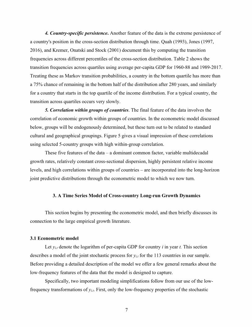
4. Country-specific persistence. Another feature of the data is the extreme persistence of

a country's position in the cross-section distribution through time. Quah (1993), Jones (1997,

2016), and Kremer, Onatski and Stock (2001) document this by computing the transition

frequencies across different percentiles of the cross-section distribution. Table 2 shows the

transition frequencies across quartiles using average per-capita GDP for 1960-88 and 1989-2017.

Treating these as Markov transition probabilities, a country in the bottom quartile has more than

a 75% chance of remaining in the bottom half of the distribution after 280 years, and similarly

for a country that starts in the top quartile of the income distribution. For a typical country, the

transition across quartiles occurs very slowly.

5. Correlation within groups of countries. The final feature of the data involves the

correlation of economic growth within groups of countries. In the econometric model discussed

below, groups will be endogenously determined, but these turn out to be related to standard

cultural and geographical groupings. Figure 5 gives a visual impression of these correlations

using selected 5-country groups with high within-group correlation.

These five features of the data – a dominant common factor, variable multidecadal

growth rates, relatively constant cross-sectional dispersion, highly persistent relative income

levels, and high correlations within groups of countries – are incorporated into the long-horizon

joint predictive distributions through the econometric model to which we now turn.

3. A Time Series Model of Cross-country Long-run Growth Dynamics

This section begins by presenting the econometric model, and then briefly discusses its

connection to the large empirical growth literature.

3.1 Econometric model

Let yi,t denote the logarithm of per-capita GDP for country i in year t. This section

describes a model of the joint stochastic process for yi,t for the 113 countries in our sample.

Before providing a detailed description of the model we offer a few general remarks about the

low-frequency features of the data that the model is designed to capture.

Specifically, two important modeling simplifications follow from our use of the low-

frequency transformations of yi,t. First, only the low-frequency properties of the stochastic

8

process need to be modeled. In particular, the stationary I(0) dynamics do not need to modeled

because the only feature of those dynamics that enters the joint distribution of the low-frequency

components is the I(0) long-run variance. The second simplification follows because the low-

frequency properties of the data are summarized by the estimated trend coefficients, which are

normally distributed in large samples. Thus, a Gaussian likelihood can be used for low-frequency

inference, so that only first two (low-frequency) moments of the process need to be modeled.

While I(0) dynamics are irrelevant over low-frequencies, highly persistent, but stationary,

dynamics are relevant. To capture these highly persistent stationary dynamics the model includes

components with autocorrelations that decay at the rate rk where r is sufficiently close to one

that rk is significantly larger than zero even when k is large, say k = 50, 100, or even 500 years.

Because of their very slow exponential decay, these are called ‘local-to-unity’ AR(1) processes,

but it should be understood that the AR(1) label refers only to the low-frequency behavior of the

process; general I(0) dynamics are allowed for the shorter-run properties of the process. We will

refer to the parameter r as the low-frequency AR parameter. For these local-to-unity processes it

is also useful to characterize persistence in terms of their half-life: for a stationary process x, the

half-life is the smallest value of h for which corr(xt, xt+h) = ½, and for a AR(1) process with AR

parameter r, the half-life solves rh = ½. Thus, a half-life of h = 100 yields r = 0.993, while h =

400 yields r = 0.998; when r is near 1, small changes in r lead to large changes in half-life.

The model is designed to capture the five key features of the data evident in the

descriptive statistics: (i) long-run global growth, (ii) low-frequency variation in that growth rate,

(iii) a roughly stationary distribution of the cross-section around the global growth factor, (iv)

highly persistent country-specific deviations from the global factor, and (v) cross-country

correlations within groups of countries. We present the model in two steps, focusing first on

cross-country covariation and then on temporal covariation.

Cross-country covariation. Common factors are used to capture low-frequency cross-

country covariation. The model includes a single common global growth factor, ft, that affects all

countries. The evolution of this factor shifts the entire cross section and is responsible for the

time-varying level of per-capita GDP in Figure 2:

yi,t = ft + ci,t, (1)

9

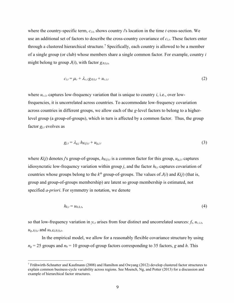
where the country-specific term, ci,t, shows country i's location in the time t cross-section. We

use an additional set of factors to describe the cross-country covariance of ci,t. These factors enter

through a clustered hierarchical structure.7 Specifically, each country is allowed to be a member

of a single group (or club) whose members share a single common factor. For example, country i

might belong to group J(i), with factor gJ(i),t,

ci,t = µc + lc,i gJ(i),t + uc,i,t (2)

where uc,i,t captures low-frequency variation that is unique to country i, i.e., over low-

frequencies, it is uncorrelated across countries. To accommodate low-frequency covariation

across countries in different groups, we allow each of the g-level factors to belong to a higher-

level group (a group-of-groups), which in turn is affected by a common factor. Thus, the group

factor gj,t evolves as

gj,t = lg,j hK(j),t + ug,j,t (3)

where K(j) denotes j's group-of-groups, hK(j),t is a common factor for this group, ug,j,t captures

idiosyncratic low-frequency variation within group j, and the factor hk,t captures covariation of

countries whose groups belong to the kth group-of-groups. The values of J(i) and K(j) (that is,

group and group-of-groups membership) are latent so group membership is estimated, not

specified a-priori. For symmetry in notation, we denote

hk,t = uh,k,t, (4)

so that low-frequency variation in yi,t arises from four distinct and uncorrelated sources: ft, uc,i,t,

ug,J(i),t and uh,K(J(i)),t.

In the empirical model, we allow for a reasonably flexible covariance structure by using

ng = 25 groups and nh = 10 group-of-group factors corresponding to 35 factors, g and h. This

7 Frühwirth-Schnatter and Kaufmann (2008) and Hamilton and Owyang (2012) develop clustered factor structures to explain common business-cycle variability across regions. See Moench, Ng, and Potter (2013) for a discussion and example of hierarchical factor structures.

10

hierarchical factor structure with up to 35 factors, and where countries are endogenously and

probabilistically assigned to groups, provides a flexible and parsimonious covariance structure

for the country-specific components, ci,t.

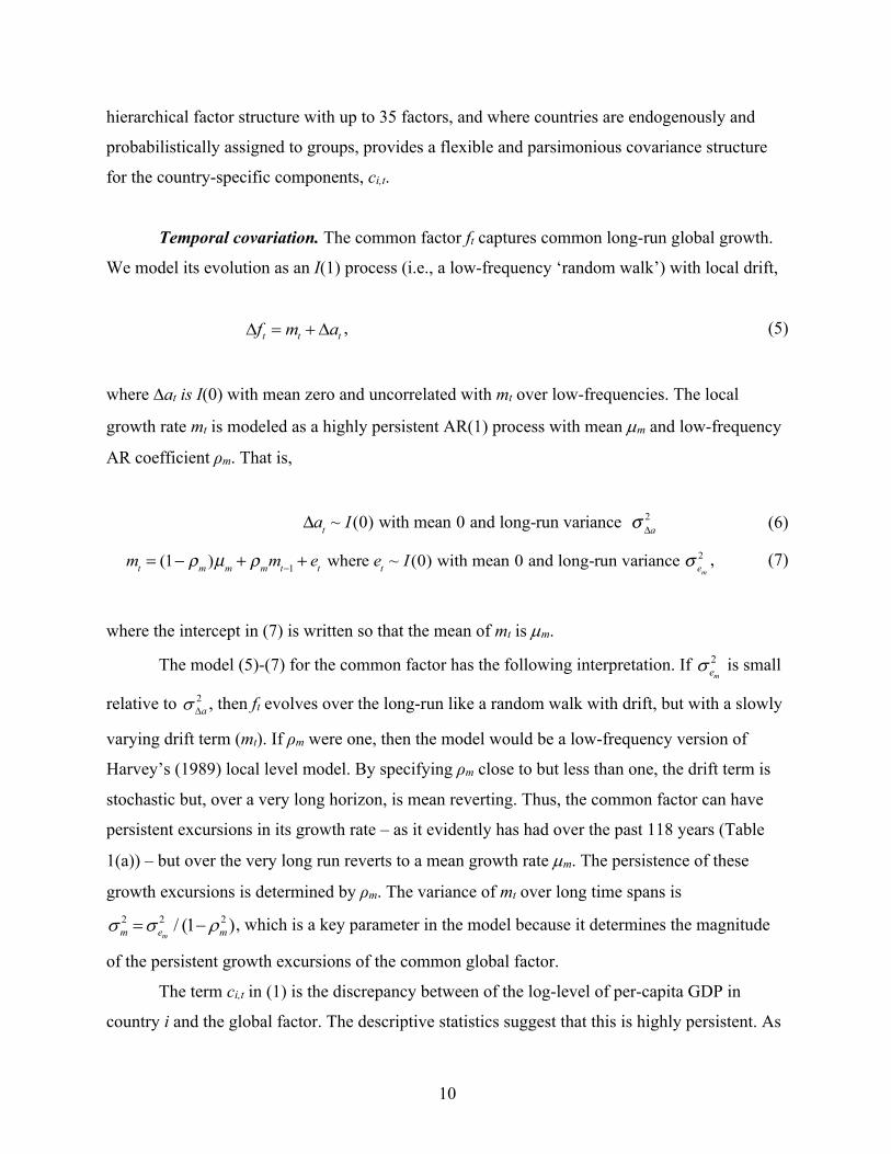
Temporal covariation. The common factor ft captures common long-run global growth.

We model its evolution as an I(1) process (i.e., a low-frequency ‘random walk’) with local drift,

, (5)

where Dat is I(0) with mean zero and uncorrelated with mt over low-frequencies. The local

growth rate mt is modeled as a highly persistent AR(1) process with mean µm and low-frequency

AR coefficient ρm. That is,

(6)

, (7)

where the intercept in (7) is written so that the mean of mt is µm.

The model (5)-(7) for the common factor has the following interpretation. If is small

relative to , then ft evolves over the long-run like a random walk with drift, but with a slowly

varying drift term (mt). If ρm were one, then the model would be a low-frequency version of

Harvey’s (1989) local level model. By specifying ρm close to but less than one, the drift term is

stochastic but, over a very long horizon, is mean reverting. Thus, the common factor can have

persistent excursions in its growth rate – as it evidently has had over the past 118 years (Table

1(a)) – but over the very long run reverts to a mean growth rate µm. The persistence of these

growth excursions is determined by ρm. The variance of mt over long time spans is

, which is a key parameter in the model because it determines the magnitude

of the persistent growth excursions of the common global factor.

The term ci,t in (1) is the discrepancy between of the log-level of per-capita GDP in

country i and the global factor. The descriptive statistics suggest that this is highly persistent. As

t t tf m aD = +D

Δat ~ I(0) with mean 0 and long-run variance σ Δa2

mt = (1− ρm )µm + ρmmt−1 + et where et ~ I(0) with mean 0 and long-run variance σ em

2

2me

s

2asD

2 2 2/ (1 )mm e ms s r= -

11

described above, variation in ci,t arises from the u random variables in (2), (3), and (4). We model

each of these variables as stationary but potentially highly persistent. Thus, over the very long

run, each country's growth is determined by ft, but slow mean reversion in ci,t provides country-

specific dynamics that are ultimately transitory but may have a half-life of several centuries.

Autoregressive component models are a convenient and flexible way to capture

persistence. We therefore model each of the ut terms as the sum of two independent low-

frequency AR(1) processes, say ut = u1,t + u2,t, with low-frequency AR coefficients r1 and r2 and

where (1-rjL)uj,t has long-run variance for j = 1, 2. Different values of (r1, r2, s1, s2) allow

for processes with, for example, a relatively quickly mean-reverting component (say, a half-life

of 30 years) and very slowly mean-reverting component (say, a half-life of 300 years). In AR

models, parameters such as rj affect both the persistence and variance of the process. To separate

persistence from variability we parameterize each ut process as

ut = su × wt (8)

wt =z w1,t + (1 - z2)1/2w2,t

wj,t = rj wj,t-1 + ej,t, j = 1, 2

where w1,t and w2,t are independent, each with a unit unconditional variance, and 0 ≤ z ≤ 1 is the

weight placed on w1,t. In this parameterization, wt has a unit variance, (r1, r2, z) describe the

persistence in ut, and su is its unconditional standard deviation.

There are 148 u-processes, corresponding to the 113 countries in (2), the 25 g-factors in

(3) and 10 h-factors in (4). We model each as an independent 2-component low-frequency AR

process with its own (r1, r2, z, su) parameters.

Relationship of the model with previous work. The model features two forms of b -

convergence familiar from the growth literature (c.f., the surveys by Durlauf and Quah (1999)

and Johnson and Papageorgiou (2018)). First, in the long run, the expected GDP paths of any

two countries i and j are expected to converge in the sense of Bernard and Durlauf (1995, 1996),

that is, limh→∞E(yi,t+h - yj,t+h | Wt) = 0, where Wt contains the history of y through time t. This

convergence obtains in the model because the country-specific terms ci,t+h and cj,t+h exhibit mean

reversion to their common mean µc, and ft has the same effect on all countries so that ft is a single

σ j2

12

common trend. While all country’s forecast paths converge to the same point, the speed of

convergence differs across countries because of the heterogeneity in the persistence parameters

(r1, r2, z). Said differently, because ci,t is stationary, in this model all countries share a single

common trend (ft), and in this sense are cointegrated. The persistence parameters might be such

that this cointegration would not be evident in any century-long sample, however.

Second, in the medium run (which in our model can be a half a century or more), the

model also features a form of conditional b - convergence (e.g., Barro (1991), Barro and Sala-i-

Martin (1992), and Mankiw, Romer and Weil (1992)) in which yi,t tends toward a growth path

with a country-specific level. The vast growth-regression literature has investigated the sources

of heterogeneity in these levels (see Sala-i-Martin (1997) for several examples and Durlauf

(2009) for a survey). In our framework, conditional convergence is captured by the AR-

component of the various u random variables that determine the evolution of ci,t. Each u term is

the sum of two independent components, the first with persistence parameter and the second

with . If is very close to unity, the first component will be very persistent, for example it

can have a half-life of several centuries. While ultimately mean reverting, this component can

vary little over, say, 50-year samples and in this sense captures the economic forces underlying

the level-shifters included in growth regressions. A smaller value of produces a component

with relatively rapid mean reversion; for example, = 0.98 produces the 2%-per year

convergence rate often found in growth regressions (see Barro (2012)).

The model also features convergence clubs discussed for example in Quah (1996, 1997).

Near unit-root dynamics for one of the AR components describing the factors gt or ht generates a

highly persistent common level component for the group of countries that load on this persistent

factor. This persistent group component could have a half-life of several centuries, so that there

could be relatively rapid convergence within the club but the club itself converges very slowly to

the global factor.

Our model generalizes the model of Raftery et al (2017), which was developed to

construct long-horizon forecasts of per-capita global GDP growth as an input to climate change

research. That model features a single common factor, proxied by the U.S., which follows a

random walk with a drift that breaks in 1973, but is otherwise constant. Their country-specific

terms (ci,t in our notation) follow independent zero-mean AR(1) processes. Relative to Raftery et

1r

2r 1r

2r

2r

13

al. (2017), the model here allows for low-frequency variation in the growth rate of the common

factor and group convergence dynamics.

There are also notable features that are not incorporated in the model. In particular the

model does not feature s-convergence, a narrowing of the cross-sectional distribution over time.

In our formulation, while we allow heterogeneity in the variance of ci,t across countries, these

variances are constant through time, so the implied variance of the cross-sectional distribution of

ci,t is time invariant. This modeling choice is based on the apparent lack of s-convergence over

the 118-year sample shown in Figures 2 and 4. In addition, the model does not incorporate non-

stationarities like those postulated in Lucas (2000) and empirically implemented in Startz (2020).

In those models, each country’s growth is governed by a two-state process that determines its

convergence to frontier economies: there is no convergence in the first state, but convergence

occurs in the second, absorbing state. Following a transition to the convergent state, poor

countries grow rapidly and inequality in income levels decreases over time. Long-run point

forecasts of future growth from this model may look much like those from the model we

implement – both feature unconditional convergence (in expectation) with a rate estimated from

historical data – but long-run predictive densities will differ because of the Lucas-Startz

framework has σ-convergence whereas ours does not. In addition, compared to those models we

allow for (data-influenced) additional variability in the long-run growth rate of the common

factor.

4. Bayes Estimation and Prediction

The challenge in specifying a model that describes the joint dynamics of 113 countries is

balancing flexibility about the many ways these variables might interact with the limited

information in the sample data. The model outlined in the last section strikes one such balance,

but at a cost of introducing more than 800 parameters, some of which are only weakly identified

by the sample data. With this in mind, we estimate the model using Bayes methods that augment

the sample data with judgment about the values of many of these 800+ parameters.

We begin by presenting the priors used in the empirical analysis. These priors are flat

(uninformative) about a handful of the model parameters, but are otherwise informative, and

therefore require discussion and justification. We then discuss how the computation of the

14

posterior and the predictive distributions takes advantages of the multiple simplifications arising

from the use of low-frequency projections combined with the linear factor structure of the model.

4.1 Priors

There are two sets of parameters in the model. One set includes parameters that are

common to all countries; this includes the initial condition f0, the mean common growth rate µm,

the persistence parameter rm, the long-run standard deviations and sm that characterize the

global factor, ft, in (5) and the parameter µc, the common mean of ci,t in (2). The other set of

parameters are country- or group-specific; this includes the factor loadings {lc,i, lg,j} in (2) and

(3) and the parameters (r1, r2, z, su) that describe the evolution of the various u random

variables in (2)-(4). We discuss these in turn.

Common parameters. We use uninformative (flat) priors for f0, µm and µc, and for

use a nearly uninformative inverse- prior that is scaled to have median equal to 0.032.

The prior for (ρm, σm) is a key informative joint prior governing the long-term distribution

of the growth of the common factor. We choose the prior for rm so that the half-life of growth

rate excursions (hm) is roughly a century. Specifically, the prior for ρm is such that the half-life hm

~ U[50, 150], approximated by a grid of 25 discrete values. For sm, we specify an independent

symmetric triangular informative prior with support 0.1 ≤ 100sm ≤ 2.0, also approximated by a

grid of 25 discrete values.

The prior mean for the long-run standard deviation of mt is 1.05 percentage points of

growth. Over the 1900-2017 sample, the mean OECD growth rate was 1.9% so a +/- one (prior)

standard deviation range around that mean is 0.9% to 2.9%. This range encompasses the 25-year

growth rates for the OECD (and the United States) tabulated in Table 1. The data turn out to be

relatively uninformative about the value of σm, and long-horizon forecast uncertainty depends on

this parameter, so this distribution is a substantive restriction that makes this prior informative

for the out-of-sample predictive distributions. We discuss sensitivity of the predictive

distributions to this prior in Section 6.

Country- and factor-specific parameters. We use a common framework for these

parameters that incorporates an exchangeable prior on a discrete support with a hierarchical

structure. Let qi, i = 1, … , m, denote a set of these parameters, for example, the set of the

asD

2asD

21c

15

country-specific factor loadings, {lc,i}, in (2), so that m = n. We specify the common support for

qi as qL ≤ qi ≤ qU, with values for q represented by nq grid points, q1, …, between the uppper

and lower bounds. Given a prior p = (p1, … , ), the prior distributions for qi are i.i.d. with

P(qi = q j) = pj, so that the number of qi ‘s taking on the value q j has a multinomial distribution.

We use a Dirichlet prior with common parameter a/nq for the multinomial probabilities, pj. That

is p ~ D(a/nq), where the parameter a is the parameter of a discrete Dirichlet process prior. With

the grid points evenly distributed in [qL, qU] and nq large, the Dirichlet prior over p with common

parameter a thus shrinks the prior over θ toward an approximately continuous uniform

distribution on [qL, qU]. Throughout, we use a =20.

This framework has two key features. First, the discrete support for qi greatly simplifies

the calculations required for the posterior, a point we discuss in more detail below. Second, the

hierarchical structure allows the data to inform the posterior for {qi} through its effect on the

posterior probability assigned to the possible values of qi, that is P(qi = q j) = pj. The Dirichlet

prior shrinks these probabilities toward a common value, but as we will see in the empirical

analysis, the data modifies this prior in interesting ways. Specifics for each set of parameters are:

• For {lc,i} in (2), qL = 0.0, qU = 0.95, with nq = 25 gridpoints evenly distributed between

these values. The same prior is used for {lg,j} in (3), with an indepedendent Dirichlet

process prior.

• The persistence parameters for the various sets of u random variables in (2), (3) and (4)

follow indpendent Dirchlet-multinomial priors. Each u is charcterized by (r1, r2, z) (see

(8)). We found it useful to parameterize the prior for these parameters in terms of the

implied half-life for the stochastic process. We specify a joint prior for (r1, r2, z) using

three independent random variables Ui ~ U(0,1), i= 1, 2, 3, and let q = (U1, U2, U3).

Denote the half-life for w1 as h1 = 25 + 775(U1)2, so that the half-life is between 25 and

800 years, and the implied value of r1 is r1 = . Define r2 similarly using U2, and

let z = U3. We construct a uniform grid on Q = [0,1]3 for (U1, U2, U3) which defines a

grid over the values of (r1, r2, z) and use nq = 100 grid points. A calculation shows that

the resulting prior shrinks the half-lives for each ut toward a distribution with 25th, 50th,

and 75th percentiles of 130, 290, and 510 years.

nqq

np q

11/(0.5) h

16

• The prior for the set of scale factors, su in (8) was calibrated relative to a homoskedastic

benchmark model. Specifically, let {su,c,i} denote the set of scale factors for the u random

variables in (2). We parameterized these as su,c,i = , and similarly for

{su,g,j}, the scale factors for the u-variables in (3), and {su,h,k} in (4). In this

parameterization, unit values of kc,i, kg,j and kh,k imply that the variance of ci,t is equal to

w2 for all i. The k parameters measure the variances of the various components relative to

this homoskedastic benchmark. For w2, we use a nearly uninformative inverse- prior

that is scaled to have median equal to 1. Priors for q = {kc,i}, {kg,j}, or{kh,k} are

independent Dirchlet-multinomial and use qL = 1/3, qU = 3 and nq = 25 evenly spaced

grid points.

• The final parameters govern the selection of countries into groups associated with the g-

factors in (2) and how these g-factor groups are further grouped using the h-factors in (3).

There are ng = 25 g-groups and nh = 10 h-groups (groups-of-groups). Let ic,j,i = 1 if

country i is a member of group j, and ig,k,j = 1 if group j is a member of group-of-group k.

We specify these as independent with P(ic,j,i = 1) = 1/ng = 1/25 and P(ig,k,j = 1) = 1/nh =

1/10.

In-sample values of ft. The final feature of the prior concerns the in-sample values of the

common global factor ft. Since ft determines the very long-run average growth in our model, it

must capture frontier growth, that is growth in the developed economies. To ensure that the in-

sample values ft accord with this interpretation, we force ft to average growth in developed

economies. We do this by imposing a prior on the in-sample values of a population-weighted

average of ci,t for OECD countries. Specifically, we assume ,

where the weights are proportional to average population of country i over 1965-1974,

scaled to sum to one. This prior shrinks the in-sample values of ft toward the population weighted

logarithm of per capita GDP of OECD countries. Since the OECD countries have no missing

data after 1950, this means that the value of ft has very little posterior uncertainty and is

effectively treated as observed over the last 65 years. We stress that this constraint is used for the

in-sample values of ft, but not the forecast out-of-sample values.

2 1/2, , ,(1 )c i c i c is l k w= -

21c

( yi,t − ft )wipop

i∈OECD∑ ~ iidN (0,0.012 )

wipop

17

4.2 Computing the posterior and predictive distributions

Various features of the model provide simplifications for the calculation of posterior. The use

of low-frequency projections of the sample data (that is, the OLS regressions of yt onto Xt from

figure 3) yields two: first, using low-frequency projections reduces the effective sample size for

each country from T annual observations, to the q+1 OLS coefficients. In this application, T is as

large as 118 and q is 16.

Second, because these OLS coefficients are low-frequency averages of the sample data with

nonrandom weights, the coefficients are approximately jointly normally distributed under quite

general conditions. We therefore use a Gaussian likelihood, which allows for analytic posterior

calculations for a subset of the model parameters and the use of conditional normal distributions

for Gibbs sampling and prediction. Specifically, let Yi denote the (qi+1) low-frequency OLS

coefficients for country i, where qi depends on sample size, which differs across countries in our

unbalanced sample. Our analysis relies on the data through Y = (Y1¢,Y2¢,…,Yn¢)¢. A central limit

result (see Müller and Watson (2019)) yields Y N(µ(q), S(q)) where q are the mean, long-run

variance and persistence parameters of the model described in Section 3.1. This normal

distribution serves as the likelihood, which together with a prior yields the posterior for the

model parameters q. Average values of yt over the forecast period (2018-2027), that is

, are also jointly normally distributed with the sample projection coefficients

Y when (k,T) are large, so . This yields the predictive density for

by averaging the N(µk(q), Sk(q)) density using the posterior for q.

A third simplifying feature is the linear factor structure of the model. Conditional on the

model parameters, linear Gaussian filtering can be used to generate draws of the factors, which

in turn can be used to obtain posterior draws of the parameters. Each of these Gibbs steps is

relatively straightforward, only involving low-dimensional multivariate normal random vectors.

The corresponding densities are easily computed by simply evaluating the associated quadratic

form for any model of time series persistence. (For the original T dimensional data, this would be

prohibitively expensive, so instead, one would need to rely on Kalman iterations or other

approaches tailored to the assumed form of persistence.)

~a

11:

1

k

T T k T ii

y k y-+ + +

=

= å

1: ( , ) ~ ( ( ), ( ))a

T T k k ky Y Nq µ q q+ + S

1: |T T k Yy + +

18

Fourth, the calculations are simplified by priors that impose a discrete support for many of

the parameters. This makes it possible to pre-compute the covariance matrices and their inverses

that are the building blocks for the various Gaussian densities used for the likelihood and Gibbs

calculations.

Finally, we treat the missing data in our unbalanced panel as missing at random.

Appendix 2 contains a detailed description of the methods we use to sample from the

posterior and predictive densities.

5. In-sample Results

The in-sample characteristics of the posterior shed light on various aspects of cross-

country growth convergence, including the speed of convergence, the heterogeneity of that

convergence, and covariance groups. These characteristics affect the long-horizon joint-

predictive distributions that are discussed in the next section. Here we first summarize the in-

sample characteristics of the global growth factor, and then turn to cross-country dynamics.

5.1 Evolution of ft

Recall that the prior (strongly) shrinks the in-sample values of ft toward a population-

weighted average of yi,t for the OECD countries, so that the resulting in-sample values of ft

roughly coincide with the logarithm of OECD per-capita GDP. This is evident in the first panel

in Figure 6, which plots the estimates of ft along with the trend components of yi,t, shaded to

differentiate OECD from non-OECD countries. The 67% error bands for ft computed from the

posterior have length of approximately 0.008, with the small value a consequence of the tight in-

sample prior.

The evolution of ft is governed by four parameters, sDa, µm, sm, and rm (see (6) and (7)).

Table 3 summarizes the posterior for these parameters. The posterior median for sDa is somewhat

lower than a typical estimate for the U.S., but this is consistent with using the OECD average for

ft. The spread of the posterior is roughly what one would find using 16 i.i.d. normal observations,

that is using q = 16 low frequency observations with Dft an i.i.d. process. The posterior for the

average growth rate, µm, is centered around 1.9% per year with 67% error bands of roughly ± 1%

per year. The second panel of Figure 6 shows the posterior estimates for mt, the local level of Dft.

19

The posterior median shows some variation over the sample, but a constant value of 1.9% (its

mean) is within the (pointwise) 67% credible set for all dates.

The long-run standard deviation sm is an important factor characterizing the evolution of

ft in the out-of-sample forecast period and therefore in determining uncertainty about the future

values of yt. The prior and posterior for sm are plotted in Figure 7. The posterior differs little

from the prior, so the data have little to say about sm at least over the support of the prior. This is

also a finding in frequentist inference on the related local-level relative variability parameter (c.f.

Stock and Watson (1997)). The posterior for the persistence in mt (parameterized using the half-

life parameter hm) is also essentially identical to its prior. (See Table 3).

5.2 Persistence and variability in ci,t

The country-specific terms ci,t are functions of uc,i,t in (2) and ug,j,t and uh,k,t for the

relevant factors in (3) and (4). Each of these u-terms has its own persistence and variance

parameters, so there are many parameters that affect the persistence and variability in each ci,t.

To summarize these effects, we focus on three characteristics of the marginal distribution of ci,t:

(i) its long-run standard deviation (sc); (ii) its half-life, the value h for which corr(ci,t, ci,t+h) = 1/2;

and (iii) the standard deviation of the change in ci,t over a 50-year span, ( ). The first two,

sc and h, are obvious ways to summarize variability and persistence. The third, ,

combines both the persistence and long-run variability of ci,t to measure the likely size of long-

run (50-year) changes in ci,t. For fixed values of sc, is decreasing in the persistence of the

process, while for fixed persistence, it is increasing in sc.

The posterior for these parameters is summarized in Table 4. The upper panel shows the

posterior pooled over the OECD and non-OECD countries. The posteriors of σc and h are plotted

in Figure 8. For both OECD and non-OECD countries the country-specific terms, ci,t, are highly

persistent, but persistence is markedly higher for the OECD countries. The median half-life

exceeds 300 years for the pooled OECD countries, but is closer to 200 years for the non-OECD

countries. The variance is also smaller for the OECD countries, and taken together, the standard

deviation of 50-year changes in ci,t are roughly 1/3 smaller for the OECD countries. Rich

countries tend to remain rich, a feature that, in part, defines inclusion in the OECD.

50( )t tc cs+ -

50( )t tc cs+ -

50( )t tc cs+ -

20

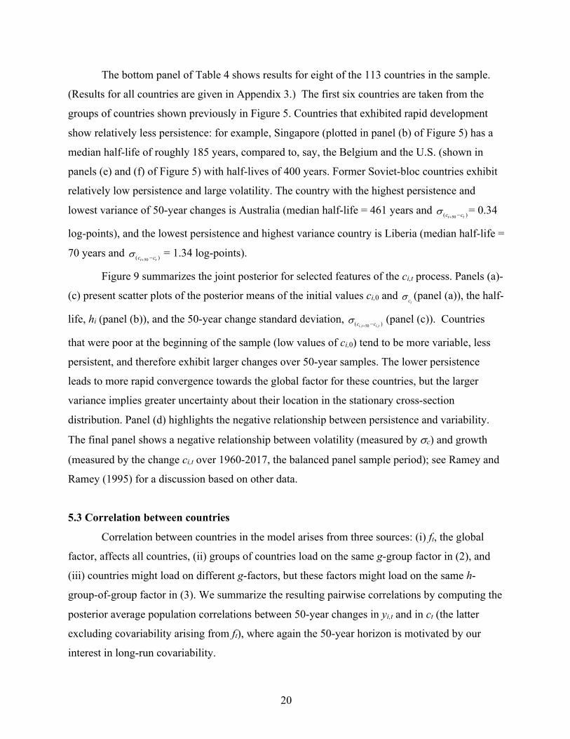
The bottom panel of Table 4 shows results for eight of the 113 countries in the sample.

(Results for all countries are given in Appendix 3.) The first six countries are taken from the

groups of countries shown previously in Figure 5. Countries that exhibited rapid development

show relatively less persistence: for example, Singapore (plotted in panel (b) of Figure 5) has a

median half-life of roughly 185 years, compared to, say, the Belgium and the U.S. (shown in

panels (e) and (f) of Figure 5) with half-lives of 400 years. Former Soviet-bloc countries exhibit

relatively low persistence and large volatility. The country with the highest persistence and

lowest variance of 50-year changes is Australia (median half-life = 461 years and = 0.34

log-points), and the lowest persistence and highest variance country is Liberia (median half-life =

70 years and = 1.34 log-points).

Figure 9 summarizes the joint posterior for selected features of the ci,t process. Panels (a)-

(c) present scatter plots of the posterior means of the initial values ci,0 and (panel (a)), the half-

life, hi (panel (b)), and the 50-year change standard deviation, (panel (c)). Countries

that were poor at the beginning of the sample (low values of ci,0) tend to be more variable, less

persistent, and therefore exhibit larger changes over 50-year samples. The lower persistence

leads to more rapid convergence towards the global factor for these countries, but the larger

variance implies greater uncertainty about their location in the stationary cross-section

distribution. Panel (d) highlights the negative relationship between persistence and variability.

The final panel shows a negative relationship between volatility (measured by sc) and growth

(measured by the change ci,t over 1960-2017, the balanced panel sample period); see Ramey and

Ramey (1995) for a discussion based on other data.

5.3 Correlation between countries

Correlation between countries in the model arises from three sources: (i) ft, the global

factor, affects all countries, (ii) groups of countries load on the same g-group factor in (2), and

(iii) countries might load on different g-factors, but these factors might load on the same h-

group-of-group factor in (3). We summarize the resulting pairwise correlations by computing the

posterior average population correlations between 50-year changes in yi,t and in ct (the latter

excluding covariability arising from ft), where again the 50-year horizon is motivated by our

interest in long-run covariability.

50( )t tc cs+ -

50( )t tc cs+ -

ics

, 50 ,( )i t i tc cs+ -

21

The average pairwise correlation between 50-year changes in log-per-capita-GDP is 0.59,

the largest pairwise correlation is between France and the Netherlands (0.97) and the smallest is

between Liberia and Bosnia and Herzegovina (0.29). The average pairwise correlation between

the country-specific terms ci,t is, of course, much smaller (0.08); the largest of these is between

France and the Netherlands (0.90), and this correlation is less than 0.01 for 38% of the country

pairs.

In many cases large pairwise correlations are associated with familiar groupings of

countries. For example, one grouping includes the early rapid developing Asian countries (Hong

Kong, Korea, Malaysia, Singapore, Taiwan, Thailand) with an average pairwise of 0.65 for ci,t.

Another includes the former Soviet-bloc countries of Bulgaria, Croatia, Hungary, Romania,

Russia, and Serbia with an average pairwise correlation of 0.66; and yet another includes the

Anglo-Saxson countries Australia, Canada, New Zealand, the US and UK with an average

pairwise correlation of 0.45.

Pairwise correlations for all countries are given in Appendix 3.

6. Predictive Distributions

This section summarizes the main findings of the paper, the long-horizon predictive

distribution of GDP-per capita for the 113 countries in the sample and various groupings of these

countries. Predictive distributions are shown for 50- and 100-year horizons. The section also

discusses sensitivity of the forecasts to changes in the priors, summarizes a pseudo-out-of-

sample experiment that checks the calibration of predictive distributions, compares the predictive

distributions from the multivariate model to the model-implied univariate predictive

distributions, and repeats the analysis using the same model and priors to compute predictive

distributions for average labor productivity (GDP per worker) instead of GDP per capita.

6.1 Baseline predictive distributions

Figure 10 shows 67% and 90% predictive intervals for the global factor ft, and for eight

representative countries. Results for all countries are shown in Appendix 3. The median of the

predictive distribution calls for the global factor to increase at an average annual rate of 1.9%

from the end of the sample in 2017 through 2118. This translates into a more than 6-fold increase

22

in the level of the global factor. The 67% prediction interval for the average growth rate is quite

wide, ranging from 0.9% to 2.7%.

The countries shown in Figure 10 illustrate the range of marginal prediction distributions.

The stationarity of ci,t implies that each country tends to mean revert to ft + µc, where µc is the

mean of ci,t in (2); countries with end-sample-values of yi,t below ft + µc will tend to grow faster

than ft and similarly for yi,t above ft + µc. The posterior for µc is summarized in Table 3; its

median is -0.6 with a 67% credible that ranges from -0.8 to -0.5 The rate at which countries

converge to this global mean is heterogeneous, so some countries are predicted to converge to

the global mean over this 100-year horizon while others do not. For example, the United States is

predicted to evolve much like the global factor, albeit with a slightly wider predictive density.

Singapore (the second richest country at the end of the sample), is predicted to grow more slowly

than average (1.4% per year over the next 100 years) as it mean-reverts down toward the growth

path of ft + µc. The end-of-sample values of yi,t for China is near ft + µc, so it is predicted to grow

at the same rate as ft; this entails a slowdown in its growth rate to that of the global factor.

Liberia has very low GDP per capita, high trend variability, and low trend persistence, so it is

predicted to revert rapidly to the global mean, however there is great uncertainty about that

prediction, and the 90% prediction interval 50 years ahead includes the possibility that its GDP

per capita fails to return even to its level in the 1960s.

Figure 11 shows prediction intervals for 50- and 100- year average growth rates for each

of the 113 countries, where the countries are ordered from poorest to richest based on end-of-

sample values of per-capita GDP. The prediction intervals shift down when moving from the

poorest to the richest country, reflecting the mean reversion (convergence) in the model which in

turn implies that poor countries are predicted to grow faster than rich countries.

A striking and important feature of the intervals in Figures 10 and 11 is their width,

which in all cases exceeds 2 percentage points for 50-year average growth for 67% prediction

intervals and is typically 5 percentage points for 90% prediction intervals. For the United States,

for example, the 67% prediction interval for average growth over the next 50 years is 0.6% to

2.7%, and over the next 100 years it is 0.7% to 2.6%.

As can be seen in Figure 11, the 100-year prediction intervals are narrower than the 50-

year intervals. For example, the average width of the 67% bands for h = 100 is 2.2 percentage

points, but is 2.7 percent points for h = 50. Increasing the horizon has two countervailing effects

23

on forecast uncertainty: on the one hand, averaging I(0) processes over longer periods reduces

variance, but variances increase for highly persistent processes like those describing mt, the local

level of f. Figure 11 indicates that the first effect dominates, at least for 50- and 100-year forecast

horizons.

Table 5 summarizes results for various groupings of countries, using end-of-sample

populations to weight the country-specific per-capita values. This weighting scheme suggests

that global per-capita income will rise by an annual rate of 2.0% of the next 100 years, resulting

a more than seven-fold increase in per-capita GDP. The degree of uncertainty is, however, very

wide, with a 67% prediction interval of 1.1% to 3.0% per year. The richer countries are predicted

to increase more slowly than the poor countries: the 67% prediction interval for 100-year per-

capita GDP growth for non-OECD countries is essentially the same as that for OECD countries,

but shifted up by 0.4 percentage points. This pattern of faster growth for the poorer countries also

can be seen in the country groupings used in the IMF's World Economic Outlook (2020), where

the median of the 100-year-ahead predictive distributions calls for an average annual growth rate

of 2.6% for Sub-Saharan Africa and 1.7% for the advanced economies.

6.2 Sensitivity

We investigated the sensitivity of the model to several key assumptions, three of which

we discuss here. The first is the prior distribution for σm, the long-run standard deviation of the

growth rate trend for ft in (5). The results are summarized in Table 6.

The parameter σm governs the extent to which the local trend growth rate of ft varies over

time, with larger values of σm admitting larger variation in the growth rate. Because we treat ft as

effectively observed (the OECD average) within sample, changes in the prior for σm have very

little effect on the in-sample results on convergence and clubs discussed in Section 5. For the

forecasts, however, larger values of σm have two important effects. First, larger values of σm

allows the posterior mean of mt to vary more and because of the slowdown in OECD growth

over the final 25 years of the sample, larger values of σm mean that the estimated (filtered) 2017

value of the local growth rate is lower, leading to a lower posterior median growth forecast.

Second, larger values of σm allow mt to vary more over the future, leading to a greater dispersion

of growth rates.

24

The second and third rows of Table 6 summarize the sensitivity of the posterior to

changes in the prior for σm, specifically shifting the prior in (towards smaller values of σm) and

out (towards larger values) by 50%. Because the data are largely uninformative about σm,

changing the prior has a large effect on the posterior for sm (Table 6(a)). Because ft is effectively

treated as observed in-sample, so is ci,t, so changing the prior on the parameters of ft has

essentially no effect on the posterior for the parameters of ci,t (Table 6(b)). When the prior favors

smaller values of σm, the predicted median growth rate increases and the spread around that

median tightens, but when the prior favors larger values of σm, the median growth rate falls and

the spread widens (Table 6(c)).

We also investigated the sensitivity of the results to q, the number of periodic terms used

to obtain the estimated country-level trend for log GDP per capita. A larger value of q includes

variation of shorter duration, for example we obtained results using q = 23 which corresponds to

a low-pass filter that extracts periodicities longer than 10 years. As seen in Table 6, using q = 23

increases the estimated variability of at (the I(1) term in the evolution of ft) but results in only

small changes in the results about persistence, convergence, and clubs discussed in Section 5.

Using q = 23 has little effect on the predictive distributions. Using the smaller value q = 9, which

corresponds to a low-pass cutoff of 26 years, yields results that are very similar to the benchmark

model of q = 16.

As another check, we re-estimated the model over the 1950-2017 sample, when we have

a nearly balanced panel. For these calculations we used q = 9, focusing on periods longer than 15

years as in the benchmark specification. The results are shown in the final row of Table 6. The

shorter sample suggests a somewhat smaller value for sDa and larger value for sm (panel (a)),

similar country-specific parameters (panel (b)) and future growth (panel (c)).

6.3 Forecasts for average labor productivity

Thus far, the focus has been on forecasting per-capita values of GDP (Y/Pop). A related

exercise focuses instead on average labor productivity (Y/L). Employment data are available in

the Penn World Table (PWT), but not the Maddison Project Database, so the sample period is

restricted to 1950-2017. We used these data and the model of Section 3 to estimate the posterior

and long-horizon predictive distribution for average labor productivity.

25

Appendix 3 contains detailed results. The final row in each panel of Table 6 summarizes

a few key results. The posteriors for the parameters using Y/L are similar to those using Y/Pop

(panels (a) and (b) of Table 6), while forecasts are for slightly slower growth and more

uncertainty.

6.3 A pseudo-out-of-sample forecasting experiment

Typically, pseudo-out-of-sample (POOS) forecasting experiments are of limited use for

evaluating long-horizon forecasts because of the limited number of independent long-horizon

POOS time-series observations. However, in our context each of the n = 113 countries provides

some independent POOS information about the validity of the predictive distribution. We have

carried out a POOS experiment that focuses on this cross-sectional information.

Specifically, in the first experiment we estimated the complete model through time T1 =

1977, and computed joint predictive distributions for the average growth rate of ft and yi,t for

each of the 113 countries over the subsequent h = 20, 30 and 40 years. The realized values of yi,t

are known over these POOS forecast periods; moreover, the realized value of ft is well

approximated by full-sample estimates ft|T (see Figure 6a). Thus, ci,t|T = yi,t - ft|T provides an

accurate estimate for the POOS out-of-sample realized value of ci,t. We therefore used ft|T and

ci,t|T to evaluate the POOS predictive distributions. Specifically, as is standard for evaluating

predictive distributions (see Diebold, Gunther and Tsay (1998)), sample values of the predictive

distributions probability integral transform (PITs) were computed by evaluating the predictive

distributions at the realized POOS values of ft|T and ci,t|T. Recall that for a correctly specified

predictive distribution, the sample values of the PIT are distributed as a U(0,1) random variables.

Table 7 summarizes the resulting PITs for the experiment, and two other experiments use

T1 = 1987 (with a forecast horizon h = 20 and 30 years) and T1 = 1997 (with a forecast horizon of

h = 20 years). Table 7 summarizes the results. These result in six forecasts for ft and with PIT

values shown in the first column of the table. This is a very small sample of dependent

observations, but the PITs provide no evidence of misspecification in the predictive distributions

for ft.

There are 113 forecasts ci,t for each POOS experiment and forecast horizon, so these

forecasts are more informative about their predictive distributions. The table summarizes the ci,t

forecasts by showing the fraction of PITs in each of the quartiles or the U(0,1) distribution:

26

ideally, 25% of the PITs should be less than 0.25, 25% should be between 0.25 and 0.50, and so

forth. The table also shows the Kolmogorov-Smirnov (KS) statistics testing the null hypothesis

that the actual values were draws from the predictive distributions (i.e., that the PITs were

U(0,1) draws). The p-values for the KS statistic were computed treating the posterior predictive

distribution as the truth, which incorporates the model-implied cross-sectional dependence in ci,t.

The results suggest that the predictive distributions for T1 = 1977 were somewhat too

optimistic: roughly half of the realized values of ci,t lie in the lower quartile of the predictive

distributions. The predictive distributions for T1 = 1987 and T1 = 1997 seem to be reasonably

well-calibrated.

6.4 Comparison of multivariate forecasts to univariate forecasts

A key feature of the simultaneous model of all countries is that the Bayesian methods

have the effect of introducing shrinkage in the parameters. Thus, the forecasts for the individual

countries reflect shrinkage to common dynamics. It is thus of interest to compare the forecasts

emerging from these joint predictive densities to univariate forecasts that do not use the

information from other countries.

We used the joint model described and prior described above to compute univariate

forecasts, constructed by treating as missing the data for all countries other than the country at

hand. The 67% 50-year ahead univariate forecast intervals are overlaid on multivariate intervals

in Figure 12. Two features are evident. First, the implied univariate intervals are typically (but

not always) substantially wider than the multivariate intervals. Second, the projections for the

lower-income countries are typically lower in the univariate than multivariate methods, and in

many cases include negative values so that the 67% interval includes 50 years of stagnation or

collapse. One driver of this difference, especially for low-income countries, is that the univariate

forecasts cannot impose the convergence that is allowed for in the multivariate forecasts, albeit

with the possibility that the convergence might be so slow that it is not evident for some

countries even in a 100-year sample.

As an illustration, the univariate and multivariate forecast intervals are shown in Figure

13 for selected countries. The univariate forecasts extrapolate country-specific in-sample

behavior, so for example the Central African Republic is predicted to continue contracting and

India and the Republic of Korea are predicted to continue their rapid growth. Indeed, the median

27

univariate forecasts imply that in 100 years, per-capita GDP in Korea will be more than six times

larger than the value in the U.S., and the univariate model produces similarly unreasonable

forecasts for other rapidly developing countries. In contrast, for several countries the univariate

forecasts are similar to the multivariate forecasts; Denmark and Ecuador, plotted in the figure,

are two examples.

7. Concluding Comments

We offer two sets of concluding comments. The first focuses on our empirical application

and the second on future applications.

In our application, the data turned out to be informative about many aspects of the

analysis. For example, it is clear that there is a wide range of rates of convergence, with some

countries having convergence half-lives of less than a century and others having half-lives so

long that, in a century-long sample, there is essentially no convergence at all. Similarly, the data

are consistent with a sparse long-run correlation pattern, that is "convergence clubs."

One aspect on which the 118 years of data on GDP per capita do not speak strongly is the

amount of persistent variation in long-term growth rate of the common factor. The long-run

standard deviation, sm, is weakly identified in the data. In our model, this weak identification

does not substantially influence our in-sample conclusions, such as those about convergence

clubs, because we treat the factor ft as essentially observed in-sample (the OECD mean). But for

forecasts 50 and 100 years ahead, the prior on sm affects both the mean growth rate of the factor

(through the estimate of its long-run growth rate today) and the spread of the predictive

distribution. We have proposed a particular prior for the value of sm that seems reasonable to us,

but others might have different priors. We provided examples of how the predictive distributions

would change for alternative candidate priors on sm. A virtue of the model is that it reduces a

seemingly overwhelming question of what is the future distribution of growth for 113 countries

over the next century to a question about a scalar parameter, the relative magnitude of the

persistent and nonpersistent changes in the growth rate of the global factor.

Finally, the modeling framework outlined here provides a flexible, yet tractable structure

for studying the joint dynamics for a large number of related time series (n = 113 countries) over

a long span (T = 118 years) with data irregularities (missing data). It yields insights about the

28

joint in-sample behavior of the series and provided sensible long-run joint prediction

distributions. This framework holds promise for delivering similar insights in other high

dimensional empirical applications involving economic time series.

29

References

Barro, R. J. (1991), “Economic Growth in a Cross-Section of Countries,” Quarterly Journal of

Economics, 106(2), pp. 407-443. Barro, R.J. (2012), “Convergence and Modernization Revisited,” NBER Working Paper 18295. Barro, R.J. and X. Sala-i-Martin (1992), “Convergence,” Journal of Political Economy, 100(2),

pp. 223-251. Bernard, A. and S.N. Durlauf. (1995), “Convergence of International Output Movements,”

Journal of Applied Econometrics, 10, 97-108. Bernard, A. and S.N. Durlauf. (1996), “Interpreting Tests of the Convergence Hypothesis,”

Journal of Econometrics, 71, 161-173. Bolt, J., R. Inklarr, H. de Jong, and J.L. van Zanden (2018), “Rebasing 'Maddison': New Income

Comparisons and the Shape of Long-Run Economic Development,” Groningen Growth and Development Centre Research Memorandum 174.

Diebold, F.X., T.A. Gunther, and A.S. Tay (1998), "Evaluating Density Forecasts with

Applications to Financial Risk Management," International Economic Review, 39(4), 863-883.

Durlauf, S.N. (2009), “The Rise and Fall of Cross-Country Regressions,” History of Political

Economy, 41, pp. 315-333. Durlauf, S.N. and D. Quah (1999), “The New Empirics of Economic Growth,” in Handbook of

Macroeconomics, J. Taylor and M. Woodford eds. North-Holland. Feenstra, R.C., R. Inklarr, and M.P. Timmer (2015), “The Next Generation of the Penn World

Tables,” American Economic Review, 105(10), pp. 3150-3182. Frühwirth-Schnatter and Kaufmann (2008), “Model-based clustering of multiple time series,

Journal of Business and Economic Statistics 26(1), 2008, 78-89. Greenstone, M., E. Kopits, and A. Wolverton (2013), “Developing a Social Cost of Carbon for

US Regulatory Analysis: A Methodology and Interpretation,” Review of Environmental Economics and Policy 7(1), 23-46.

Harvey, A.C., Forecasting, Structural Time Series Models and the Kalman Filter. Cambridge

UK: Cambridge University Press, 1989. Hamilton, J.D. and M.T. Owyang (2012), “The Propagation of Regional Recessions,” Review of

Economics and Statistics, 94(4), pp. 935-947.

30

Hausmann, R., L. Pritchett, and D. Rodrik. (2005). “Growth Accelerations,” Journal of Economic Growth, 10, 303-329.

International Monetary Fund (2020), World Economics Outlook, 2020. Johnson, P. and C. Papageorgiou (2018), “What Remains of Cross-Country Convergence?”

Journal of Economic Literature, forthcoming. Jones, B.F. and B.A Olken. (2008). “The Anatomy of Start-Stop Growth,” Review of Economics

and Statistics, 90, 582–587. Jones, C.I. (1997), “On the Evolution of the World Income Distribution,” Journal of Economic

Perspectives, 11(3), pp. 19-36. Jones, C.I. (2016), “The Facts of Economic Growth,” in Handbook of Macroeconomics, Vol. 2A,

J.B. Taylor and H. Uhlig (eds), pp. 3-68. Kremer, M., A. Onatski and J.H. Stock (2001), “Searching for Prosperity,” Carnegie Rochester

Conference Series on Public Policy, 55, pp. 275-303. Lucas, R.E. (2000), “Some Macreconomics for the 21st Century,” Journal of Economic

Perspectives, 14(1), pp. 159-168. Maddison, A. (2007). Contours of the World Economy, 1-2030AD: Essays in Macro-Economic

History, Oxford University Press. Mankiw, N.G., D. Romer and D.N. Weil (1992), “A Contribution to the Empirics of Economic

Growth,” Quarterly Journal of Economics, 107(2), pp. 407-437. Moench, E., S. Ng and S. Potter (2013), “Dynamic Hierarchical Factor Models,” Review of

Economics and Statistics, 95(5), pp. 1811-1817. Müller, U.K. and M.W. Watson (2008), “Testing Models of Low-Frequency Variability,”,

Econometrica, Vol. 76, No. 5 (September, 2008), 979–1016. Müller, U.K. and M.W. Watson (2016), “Measuring Uncertainty about Long-Run Predictions,”

Review of Economic Studies, 83 (4), October 2016, pp. 1711-1740. Müller, U.K. and M.W. Watson (2017), “Low-Frequency Econometrics,” in Advances in

Economics and Econometrics Vol. II, B. Honore, A. Pakes, M. Piazzesi, and L. Samuelson (eds). Cambridge University Press.

Müller, U.K. and M.W. Watson (2018), “Long-run Covariability,” Econometrica, Vol. 86, No.3,

pp. 775-804.

31

Müller, U.K. and M.W. Watson (2019), “Low-Frequency Analysis of Economic Time Series,” in preparation for Handbook of Economics Vol. 7, S. Durlauf, L.P. Hansen, J.J. Heckman and R. Matzkin (eds). North Holland.

National Academy of Sciences, Committee on Assessing Approaches to Updating the Social

Cost of Carbon, Cropper M.L. and Newell, R.G. co-chairs (2017). Valuing Climate Changes: Updating Estimation of the Social Cost of Carbon Dioxide. National Academies Press at http://www.nap.edu/24651.

Pritchett, L. (2000). “Understanding Patterns of Economic Growth: Searching for Hills among

Plateaus, Mountains, and Plains,” World Bank Economic Review, 14, 221-225. Quah, D. (1993), “Empirical Cross-Section Dynamics in Economic Growth,” European

Economic Review, 37, pp. 426-434. Quah, D. (1996), “Twin Peaks: Growth and Convergence in Models of Distribution Distribution

Dynamics,” Economic Journal, 106, pp. 1045-1055. Quah, D. (1997), “Empirics for Growth and Distribution” Polarization, Stratification, and

Convergence Clubs,” Journal of Economic Growth, 2(1), pp. 27-59. Raftery, A.E., A. Zimmer, D.M.W. Frierson, R. Startz, and P. Liu (2017), “Less than 2o C

Warming by 2100 Unlikey,” Nature: Climate Change, 7(9), pp. 637-641. Ramey, G. and V.A. Ramey (1995), “Cross-Country Evidence on the Link Between Volatility

and Growth,” American Economic Review, 85(1), pp. 1138-1151. Sala-i-Martin, X. (1997), “I Just Ran Two Million Regressions,” American Economic Review

Papers and Proceedings, 82(2), pp. 178-183. Startz, R. (2020), “The Next Hundred Years of Growth: Growth and Convergence,” Journal of

Applied Econometrics, vol. 35. Stock, J.H. and M.W. Watson (1998), “Asymptotically Median Unbiased Estimation of

Coefficient Variation in a Time Varying Parameter Model,” Journal of the American Statistical Association, 93, pp. 349-358.

32

Figure 1: Countries included in data set (shown as shaded areas on map)

Figure 2: GDP per-capita for 113 countries

Notes: The thick black curve is OECD GDP per-capita, computed for those countries in the OECD in 2017 that have data available in the indicated year.

1900 1920 1940 1960 1980 2000 2020Year

102

103

104

105

2011

US

Dol

lars

33

Figure 3: Low-frequency regressors (Xt) and the logarithm of GDP per capita (yi,t) and estimated trends ( ) for selected countries

(a) Selected series with data over 1900-2017 (full sample)

(b) Selected series with data over 1950-2017

(c) Series with data over 1929-1938 and 1950-2017

yi,t

34

Figure 4: GDP per-capita for 113 countries: Trend components

Notes: The thick black curve is OECD GDP per-capita, computed for those countries in the OECD in 2017 that have data available in the indicated year.

1900 1920 1940 1960 1980 2000 2020Year

102

103

104

10520

11 U

S D

olla

rs

35

Figure 5: Selected five-country groups (low-frequency transformed data)

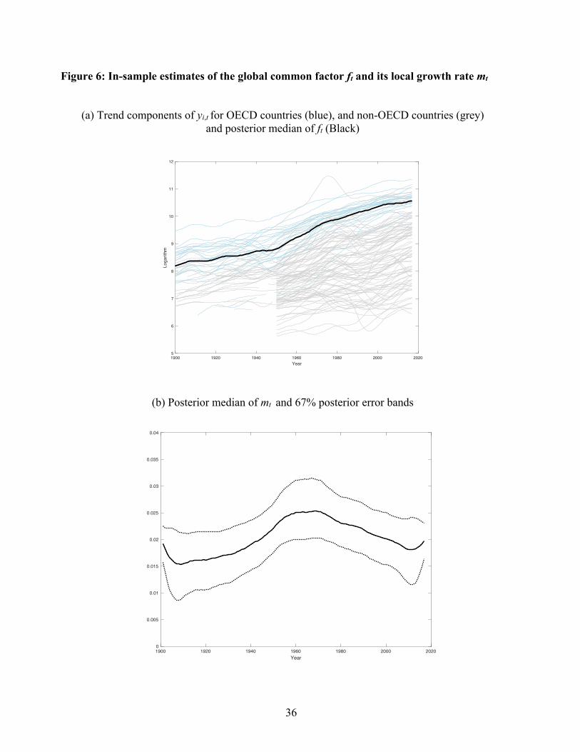
36

Figure 6: In-sample estimates of the global common factor ft and its local growth rate mt

(a) Trend components of yi,t for OECD countries (blue), and non-OECD countries (grey) and posterior median of ft (Black)

(b) Posterior median of mt and 67% posterior error bands

1900 1920 1940 1960 1980 2000 2020Year

5

6

7

8

9

10

11

12Logarithm

1900 1920 1940 1960 1980 2000 2020Year

0

0.005

0.01

0.015

0.02

0.025

0.03

0.035

0.04

37

Figure 7. Prior and posterior for sm

Figure 8. Posterior distribution of the long-run standard deviation σc and half-life h of ci,t for OECD and non-OECD countries

(a) σc

(b) h

0 0.002 0.004 0.006 0.008 0.01 0.012 0.014 0.016 0.018 0.02

m

0

0.01

0.02

0.03

0.04

0.05

0.06

0.07

0.08

Probability

PriorPosterior

38

Figure 9: Cross-country relation between initial conditions, half-life, variability and growth

Notes: Scatterplots are of the posterior means of the indicated parameters, where each observation is a country.

-2 -1 0 1c0

0.8

0.9

1

1.1

1.2

1.3

1.4

1.5

1.6

c

(a) c0 and c

-2 -1 0 1c0

0

100

200

300

400

500

half-

life

(b) c0 and half-life

-2 -1 0 1c0

0.2

0.4

0.6

0.8

1

1.2

1.4

(ct+

50-c

t)

(c) c0 and (ct+50-c t)

0 100 200 300 400 500half-life

0.8

0.9

1

1.1

1.2

1.3

1.4

1.5

1.6

c

(d) half-life and c

-2 -1 0 1 2c2017 - c 1960

0.8

0.9

1

1.1

1.2

1.3

1.4

1.5

1.6

c

(e) c2017 - c1960 and c

39

Figure 10: 67% and 90% prediction intervals for per-capita GDP Global factor and selected countries

Notes: Dark shaded areas are 67% prediction intervals; 90% intervals include the light shaded areas. Median forecasts are shown as solid lines. The in-sample value of the global factor and its median forecast are shown in each panel.

40

Figure 11: 67% and 90% prediction intervals for average growth rates Countries ordered from poorest to richest at end sample

(a) Average growth rate over next 50 years

(b) Average growth rate over next 100 years

41

Figure 12: Univariate (blue) and Multivariate (red) 67% prediction intervals for average growth rates over next 100 years:

Countries ordered from poorest to richest at end sample

42

Figure 13: Median, 67% and 90% prediction intervals for per-capita GDP: Multivariate (red line and shaded regions) and Univariate (blue line, dashes and dots)

43

Table 1: Selected summary statistics

(a) Mean growth rates of GDP per capita over 30-year periods (annual percentage growth rates)

1901-1930 1931-1960 1961-1990 1991-2017 United States 1.4 2.2 2.5 1.5

OECD 1.2 2.0 2.9 1.4 non-OECD 1.4 1.8 2.1 3.0

all 1.3 1.9 2.1 1.9

(b) Cross-sectional distribution of yi,t in selected years (logarithm of GDP per capita)

Average value of yi,t over

Cross-section median

Cross-section standard deviation

Cross-section Inter-quantile range:

75%-25% 90%-10% 1950 - 1954 7.8 1.0 1.5 2.5 1971 - 1975 8.3 1.1 1.8 2.9 1992 - 1996 8.6 1.3 2.0 3.5 2013 - 2017 9.3 1.2 2.1 3.3

Table 2: Averages of yi,t over 29 year periods: Fraction of countries of moving from growth quartile i (1960-1988) to quartile j (1989-2017)

Quartile in 1989-2017 1 2 3 4 Quartile in 1960-1988

1 0.79 0.21 0 0 2 0.21 0.68 0.11 0 3 0 0.11 0.71 0.18 4 0 0 0.18 0.82

44

Table 3: Posterior percentiles for selected parameters, ft and ct processes

Parameter Percentiles of Posterior 0.05 0.17 0.50 0.84 0.95

(a) Parameters for ft process (in percentage points) sDa 2.34 2.70 3.33 4.14 4.87 µm -0.08 0.77 1.85 2.79 3.56 sm 0.42 0.73 1.13 1.52 1.76 hm 50 63 96 133 146

(b) Parameters for c process µc -0.97 -0.83 -0.63 -0.45 -0.32

Notes: Dft = mt + Dat, where Dat is I(0) and mt is a low-frequency AR(1) with mean µm and low-frequency AR coefficient ρm. The half-life, hm, solves .

Table 4: Posterior percentiles for selected parameters, ci,t process

Half-life sc

Percentiles of Posterior 0.17 0.50 0.84 0.17 0.50 0.84 0.17 0.50 0.84

(a) Pooled across countries All countries 130 233 389 0.85 1.10 1.37 0.45 0.63 0.86 OECD 201 338 486 0.74 0.91 1.15 0.35 0.44 0.58 Non-OECD 121 211 342 0.91 1.15 1.40 0.52 0.68 0.89

(b) Selected countries China 150 222 330 1.00 1.20 1.40 0.59 0.68 0.79 Singapore 111 185 291 0.92 1.13 1.34 0.61 0.72 0.86 Madagascar 148 214 317 1.08 1.24 1.42 0.61 0.72 0.85 Belgium 286 394 507 0.69 0.82 0.98 0.32 0.37 0.44 Russia 78 138 239 0.90 1.10 1.34 0.66 0.79 0.94 United States 303 413 529 0.75 0.89 1.06 0.34 0.39 0.45 Australia 340 461 567 0.71 0.84 1.00 0.30 0.34 0.40 Liberia 50 70 108 1.36 1.51 1.62 1.17 1.34 1.50

1/ 2mhmr =

50( - )t tc cs+

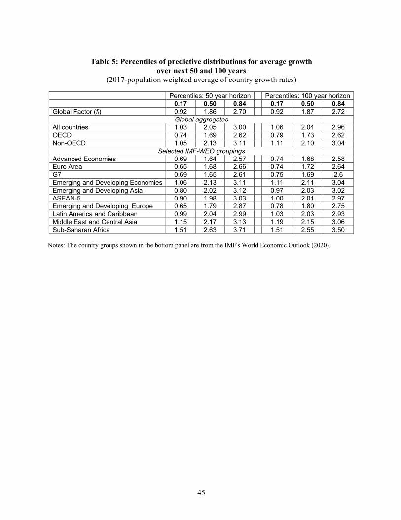
45

Table 5: Percentiles of predictive distributions for average growth

over next 50 and 100 years (2017-population weighted average of country growth rates)

Percentiles: 50 year horizon Percentiles: 100 year horizon 0.17 0.50 0.84 0.17 0.50 0.84 Global Factor (ft) 0.92 1.86 2.70 0.92 1.87 2.72

Global aggregates All countries 1.03 2.05 3.00 1.06 2.04 2.96 OECD 0.74 1.69 2.62 0.79 1.73 2.62 Non-OECD 1.05 2.13 3.11 1.11 2.10 3.04

Selected IMF-WEO groupings Advanced Economies 0.69 1.64 2.57 0.74 1.68 2.58 Euro Area 0.65 1.68 2.66 0.74 1.72 2.64 G7 0.69 1.65 2.61 0.75 1.69 2.6 Emerging and Developing Economies 1.06 2.13 3.11 1.11 2.11 3.04 Emerging and Developing Asia 0.80 2.02 3.12 0.97 2.03 3.02 ASEAN-5 0.90 1.98 3.03 1.00 2.01 2.97 Emerging and Developing Europe 0.65 1.79 2.87 0.78 1.80 2.75 Latin America and Caribbean 0.99 2.04 2.99 1.03 2.03 2.93 Middle East and Central Asia 1.15 2.17 3.13 1.19 2.15 3.06 Sub-Saharan Africa 1.51 2.63 3.71 1.51 2.55 3.50

Notes: The country groups shown in the bottom panel are from the IMF's World Economic Outlook (2020).

46

Table 6. Sensitivity of selected results to the prior for γ, the number of low-frequency periodic functions used (q), and using Y/L in place of Y/Pop.

(a) Posterior for f process (in percentage points)

Prior for sm q Start Date

sDa sm

Percentiles of posterior Percentiles of posterior 0.17 0.50 0.84 0.17 0.50 0.84

Baseline 16 1900 2.70 3.33 4.14 0.73 1.13 1.52 0.5 × Baseline 16 1900 2.95 3.55 4.3 0.33 0.56 0.76 1.5 × Baseline 16 1900 2.52 3.10 3.84 1.1 1.69 2.29

Baseline 9 1900 1.91 2.91 4.19 0.81 1.29 1.68 Baseline 23 1900 3.40 3.95 4.66 0.65 1.05 1.52 Baseline 9 1950 1.25 1.76 2.57 1.05 1.37 1.68

Using Y/L instead of Y/Pop Baseline, 1950-2017 9 1950 1.22 1.78 2.71 1.13 1.45 1.76

(b) Posterior for c process (pooled across all countries) Prior for sm q Start

Date Half-life (years)

Percentiles of posterior Percentiles of posterior 0.17 0.50 0.84 0.17 0.50 0.84

Baseline 16 1900 130 233 389 0.44 0.63 0.86 0.5 × Baseline 16 1900 129 232 387 0.45 0.63 0.86 1.5 × Baseline 16 1900 130 233 391 0.45 0.63 0.86

Baseline 9 1900 107 209 398 0.43 0.66 0.94 Baseline 23 1900 137 245 395 0.44 0.60 0.82 Baseline 9 1950 120 229 438 0.39 0.66 0.92

Using Y/L instead of Y/Pop Baseline, 1950-2017 9 1950 119 252 479 0.35 0.61 0.91

(c) 100-year-ahead predictive distributions for average growth rates (PAAR) Prior for sm q Start

Date Global Factor (ft) 2017-population weighted

average of country growth rates

Percentiles of posterior Percentiles of posterior 0.17 0.50 0.84 0.17 0.50 0.84

Baseline 16 1900 0.92 1.87 2.72 1.06 2.04 2.96 0.5 × Baseline 16 1900 1.34 1.97 2.64 1.45 2.17 2.87 1.5 × Baseline 16 1900 0.53 1.75 2.88 0.69 1.95 3.11

Baseline 9 1900 0.65 1.67 2.63 0.85 1.92 2.91 Baseline 23 1900 0.97 1.89 2.81 1.09 2.04 3.01 Baseline 9 1950 0.86 1.84 2.75 1.03 2.05 3.02

Using Y/L instead of Y/Pop Baseline 9 1950 0.65 1.72 2.70 0.75 1.85 2.96

σ (ct+50-ct )

47

Table 7. Summary of probability integral transforms for pseudo-out-of-sample forecasts

Forecast Horizon

PITs

f Fraction of c-PITs between 0 – 0.25 0.25-0.50 0.50-0.75 0.75-1.00 KS-c (p-value)

(a) T1 = 1977 20 years 0.41 0.57 0.14 0.18 0.11 0.36 (0.01) 30 years 0.38 0.50 0.15 0.19 0.16 0.28 (0.06) 40 years 0.30 0.46 0.17 0.17 0.20 0.23 (0.14)

(b) T1 = 1987 20 years 0.30 0.30 0.31 0.22 0.17 0.15 (0.42) 30 years 0.20 0.27 0.26 0.28 0.19 0.09 (0.83)

(c) T1 = 1997 20 years 0.24 0.12 0.29 0.29 0.29 0.14 (0.47)