An Econometric Analysis of Brand-Level Strategic Pricing Between ...

An Econometric Analysis of Brand-LevelStrategic Pricing Between Coca-Cola

Company and PepsiCo.

TIRTHA DHAR

Sauder School of BusinessUniversity of British Columbia

Vancouver, BC V6T1Z2Canada

[email protected]

JEAN-PAUL CHAVAS

Department of Agricultural and Applied EconomicsUniversity of Wisconsin-Madison

Madison, WI [email protected]

RONALD W. COTTERILL

Department of Agricultural and Resource EconomicsUniversity of Connecticut

Storrs, CT [email protected]

BRIAN W. GOULD

Department of Agricultural and Applied EconomicsUniversity of Wisconsin-Madison

Madison, WI [email protected]

We investigate market structure and strategic pricing for leading brands soldby Coca-Cola Company and PepsiCo. in the context of a flexible demandspecification (i.e., nonlinear AIDS) and structural price equations. Our flexibleand generalized approach does not rely upon the often used ad hoc linearapproximations to demand and profit-maximizing first-order conditions, and

This research was supported by a USDA CSRS grant 2002-06090 to the Food SystemResearch Group, University of Wisconsin-Madison and USDA CSRS Grant 00-34178-9036to the Food Marketing Policy Center, University of Connecticut. The authors are greatlyindebted to the FMPC - University of Connecticut for providing access to the data used inthe analysis. Any errors and omissions are the sole responsibility of the authors. A versionof the paper was presented at the 5th INRA-IDEI conference on Industrial Organizationand Food Processing Industries, Toulouse, France, June 20002.

c© 2005 Blackwell Publishing, 350 Main Street, Malden, MA 02148, USA, and 9600 Garsington Road,Oxford OX4 2DQ, UK.Journal of Economics & Management Strategy, Volume 14, Number 4, Winter 2005, 905–931

906 Journal of Economics & Management Strategy

the assumption of Nash-Bertrand competition. We estimate a conjecturalvariation model and test for different brand-level pure strategy games. Thisapproach of modeling market competition using the nonlinear Full InformationMaximum Likelihood (FIML) estimation method provides insights into thenature of imperfect competition and the extent of market power. We findno support for a Nash-Bertrand or Stackelberg Leadership equilibrium inthe brand-level pricing game. Results also provide insights into the uniquepositioning of PepsiCo.’s Mountain Dew brand.

1. Introduction

In this paper, we develop and estimate a structural model of brand-level competition between firms using a flexible nonlinear demandsystem and relaxing the usual assumption of Bertrand price competition.Analysis of strategic behavior of firms using structural models is widelyused in the new empirical industrial organization (NEIO) literature.The basic approach is to specify and estimate market-level demand andcost specifications after taking into account specific strategic objectivesof firms. Empirical implementation of these models is complex dueto the highly nonlinear nature of flexible demand and cost functionsand the specification of strategic firm behavior. As a result, researchershave tended to simplify structural models by specifying ad hoc orapproximated demand specifications, and reduced form conditions ofthe firm’s objectives. In this paper, we attempt to overcome some ofthese shortcomings.

In empirical structural models, the estimation of market powerand strategic behavior depends crucially on the estimated price andexpenditure elasticities. A major problem with ad hoc demand spec-ifications is that they do not satisfy all the restrictions of consumertheory.1 As a result, estimated parameters may violate basic tenets ofeconomic rationality. Even if a strategic game is correctly specified, anymisspecification of demand may generate spurious results and incorrectpolicy prescriptions due to incorrect elasticity estimates.

Researchers have tried to overcome these shortcomings of demandspecification by specifying flexible demand functions based on well-behaved utility functions. For example, Hausman et al. (1994) and Cot-terill et al. (2000) use a linear approximation to the almost ideal demandsystem (LA-AIDS; see Deaton and Muellbauer, 1980a). In this paper useof AIDS provides more flexibility as we avoid linear approximation tononlinear price effects.

1. For example, Gasmi et al. (1992, hereafter GLV) and Golan et al. (2000) use ad hoclinear demand specifications.

Strategic Pricing Between Coca-Cola Co. and PepsiCo. 907

To avoid such approximated and ad hoc demand specification,there is another strand of the NEIO literature that uses characteristicbased demand system based on the random utility model (Nevo, 2001;Villas-Boas and Zhao, 2005). Empirically this approach is appealingbecause its parsimonious description enables one to avoid specifying theprices of all brands with the attendant multicolliniarity and parameterestimation problems. However, specification of random utility modelsoften imposes restrictions that may not be implied by general utilitytheory. In a recent paper, Bajari and Benkard (2003) show that manystandard discrete choice models have the following undesirable prop-erties: as the number of product increases, the compensating variationfor removing all of the inside goods tends to infinity, all firms in aBertrand–Nash pricing game have markups that are bounded awayfrom zero, and for each good there is always some consumer that iswilling to pay an arbitrarily large sum for the good. These propertiesalso imply that a discrete choice demand curve is unbounded forany price level. To avoid this problem, Hausman (1997) uses linearand quadratic approximations to the demand curve in order to makewelfare calculations (e.g., multi stage demand system with LA-AIDS atthe last stage), favoring them over the CES specification, which hasan unbounded demand curve. Another advantage of an AIDS typedemand system is that it avoids the arbitrary and strong assump-tion of single unit purchases in the discrete choice demand model(Dube, 2004).2

In terms of specifying behavioral rules for a firm, two broadapproaches can be found in the empirical literature. Gasmi et al. (1992,GLV hereafter), Kadiyali et al. (1996) and Cotterill and Putsis (2001) havederived and estimated profit-maximizing first-order conditions underthe assumption of alternative games (e.g., Bertrand or Stackelberg)along with their demand specifications. However, these studies deriveestimable first-order conditions based on approximate demand speci-fications. Cotterill et al. (2000) use the more flexible LA-AIDS but theyapproximate the profit-maximizing first-order condition with a first-order log-linear Taylor series expansion. Implications of using suchapproximated first-order conditions have not been fully explored.

In the other strand of the empirical literature, researchers donot specify the first-order conditions. Instead, they rely on featuresof the panel data to obtain instruments for endogenous prices when

2. The purpose of our discussions on comparative advantages and disadvantages ofdifferent demand systems is not to make the claim that AIDS is the best in all situations.We seek only to justify our choice of model specification. Choice of specification issituation-specific and further research is needed to rigorously compare advantages anddisadvantages of different demand systems.


estimating the demand system (e.g., Hausman et al., 1994; Nevo, 2001).The advantage of this approach is that it avoids the pitfall of deriving andestimating complicated first-order conditions. But in terms of estimatingmarket power and merger simulation, this approach restricts itself toBertrand conjectures and the assumption of constant marginal costs(Werden, 1996).

We overcome some of these shortcomings by specifying a fullyflexible nonlinear almost ideal demand specification (AIDS) and derivethe corresponding structural first-order conditions for profit maximiza-tion. Unlike Cotterill et al. (2000), our derived first-order conditionsare generic and avoid the need for linear approximation. As a result,they can be estimated with any flexible demand specification that hasclosed-form analytical elasticity estimates. We propose to estimate oursystem (i.e., the demand specification and first-order conditions) usingfull information maximum likelihood (FIML).

In this paper, we also test for different stylized strategic games,namely Nash equilibrium with Bertrand or Stackelberg conjectures, andcollusive games. In the empirical analysis of market conduct, the correctstrategic model specification may be as critical as the demand and costspecification. Until now most antitrust analyses of market power havetended to assume Bertrand price conjectures (Cotterill, 1994; Werden,1996). One exception is Cotterill et al. (2000), who test for Bertrandand Stackelberg game at the product-category level. They test withina product category (e.g., breakfast cereal) for Stackelberg and Bertrandgames between two aggregate brands: private label and national brand.As a result, their analysis is based on a “two-player game.” Similarly,GLV (1992) estimate and test for strategic behavior of Coke and Pepsibrands. In this paper, we consider games with multiple firms andmultiple brands. In such a market, a firm may dominate a segmentof the market with one brand and then follow the competing firm inanother segment of the market with another brand. So, the number ofpossible games that need to be tested increases greatly. To the best ofour knowledge, this is the first study to test for strategic brand-levelcompetition using conjectural variation approach for multiple brandsand multiple firms.

In this paper, we also control for expenditure endogeneity inthe demand specification. Most papers in the industrial organizationliterature have failed to address this issue. Dhar et al. (2003) and Blundelland Robin (2000) have found evidence that expenditure endogeneityis significant in demand analysis and can have large effects on theestimated price elasticities of demand.

Empirically, we study the nature of price competition between thefour major brands marketed by PepsiCo. and Coca-Cola Company GLV’


(1992) study was one of the first papers to estimate a structural modelfor the carbonated soft drink industry (CSD). They developed a strategicmodel of pricing and advertising between Coke and Pepsi using demandand cost specification. Compared to the GLV study, our database is moredisaggregate. As a result, we are able to control for region-specific unob-servable effects on CSD demand. In addition, we incorporate two otherbrands produced by Coca-Cola Company and PepsiCo.: Sprite for Coca-Cola Company, and Mountain Dew for PepsiCo. Of the four brands,three are caffeinated (Coke, Pepsi, and Mountain Dew) and one is aclear noncaffeinated drink (Sprite).3 Characteristically, Mountain Dewis quite unique. In terms of taste, it is closer to Sprite but due to caffeinecontent, consumers can derive an alertness response similar to Coke andPepsi.4 These four brands dominate the respective portfolios of the twofirms.

In the present study, unlike the GLV (1992) and Golan et al. (2000)studies, we do not model strategic interactions of firms with respect toadvertising. Due to lack of city- and brand-specific data on advertising,we were unable to account for strategic interactions in advertisement(although we do control for the cost of brand promotion in our structuralmodel). Our analysis is based on quarterly IRI (Information ResourcesInc.)-Infoscan scanner data of supermarket sales of carbonated non-diet soft drinks (hereafter CSD) from 1988-Q1 to 1989-Q4 for 46 majormetropolitan cities across the United States.5

The paper is organized as follows. First, we present our conceptualapproach. Second, we discuss our model selection procedures. Third,we present our empirical model specification. Fourth, econometric andstatistical test results are presented. And finally we draw conclusionsfrom this study.

2. Model Specification

We specify a brand-level nonlinear almost ideal demand system (AIDS)model. We then derive the first-order conditions for profit maximizationunder alternative game-theoretic assumptions. Finally, we estimate themodel using a FIML procedure.

3. In terms of caffeine content, for every 12 oz. of beverage Coke has 34 mg, Pepsi has40 mg and Mountain Dew has the most with 55 mg of caffeine.

4. During the period of our study, Coca-Cola Company did not have any specific brandto compete directly against Mountain Dew. Only in 1996, they introduced the brand Surgeto compete directly against Mountain Dew.

5. Information Resources Inc., collects data from supermarkets with more than$2 million in sales from major US cities. These supermarkets account for 82% of grocerysales in the US.


2.1 Overview of the AIDS Demand Specification

This is the first study to use nonlinear AIDS in analyzing strategic brand-level competition between firms. In this section, we briefly describederivation of AIDS.

Our derivation of AIDS is based on Deaton and Muellbauer (1980b)and assumes that the expenditure function E(p, u) ≡ Minx{p′x : U(x) ≥u, x ∈ RN

+} takes the general form

E(p, u) = exp[a (p) + ub(p)], (1)

where U(x) is the consumer’s utility function, x = (x1, . . . , xN)′ is(N × 1) vector of consumer goods, p = (p1, . . . , pN)′ is a (N × 1) vectorof goods prices for x, M denotes total expenditure on these N goods,u is a reference utility level, a (p) = δ + α′ ln(p) + 0.5 ln(p)′� ln(p), α =(α1, . . . , αN)′ is a (N × 1) vector,

� =

γ11 · · · γ1N

.... . .

...γN1 · · · γNN

is a (N × N) symmetric matrix, and b(p) = exp[∑N

i=1 βi ln(pi )]. UsingShephard’s lemma, differentiating the log of expenditure function ln(E)with respect to ln(p) generates the AIDS specification,

wilt = αi +N∑

j=1

ln(pjlt) + βi ln(Mlt/Plt), (2)

where wilt = (piltxilt/Mlt) is the budget share for the ith commodityconsumed in the lth city at time t. The term P can be interpreted asa price index defined by

ln(Plt) = δ +N∑

m=1

αm ln(pmlt) + 0.5N∑

m=1

N∑j=1

γmj ln(pmlt) ln(pjlt). (3)

The above AIDS specification can be modified to incorporate theeffects of socio-demographic variables (Z1lt, . . . , ZKlt) on consumptionbehavior, where Zklt is the kth socio-demographic variable in the lthcity at time t, k = 1, . . . , K. Under demographic translating, assume thatαi takes the form αilt = α0i + ∑K

k=1 λik Zklt, i = 1, . . . , N. Then, the AIDSspecification (2) becomes


wilt = α0i +K∑

k=1

λik Zklt +N∑

j=1

γmj ln(pjlt) + βi ln(Mlt)

− βi

[δ +

N∑m=1

α0m ln(pmlt) +N∑

m=1

K∑k=1

λmk Zklt ln(pmlt)

+ 0.5N∑

m=1

N∑j=1

ln(pmlt) ln(pjlt)

]. (4)

The theoretical restrictions are composed of symmetry restrictions,

γi j = γ j i for all i �= j

and homogeneity restrictions,

N∑i=1

α0i = 1;N∑

i=1

λik = 0, ∀k;N∑

i=1

γi j = 0, ∀ j ; andN∑

i=1

βi = 0. (5)

The system of share equations represented by (4) is nonlinear in theparameters. The parameter δ can be difficult to estimate and is often setto some predetermined value (Deaton and Muellbauer, 1980b). For thepresent analysis, we follow the approach suggested by Moschini et al.(1994) and set δ = 0.

2.2 Derivation of the Profit-MaximizingFirst-order Conditions

Conjectural variation (CV) models have been widely used in theoret-ical and empirical modeling and in analyzing the comparative staticof different strategic games of firms (see, e.g., Brander and Spencer,1985; Dixit, 1986; Genesove and Mullin, 1998). CV parameters areinterpreted as an intuitive summary measure of market conduct, andas a result in existing empirical literature they are sometimes termedconduct parameters (Brander and Zhang, 1990). Our model based onCV parameters is in the same spirit. Because CV models nest most ofthe noncooperative games that we investigate (see below), they helpsimplify the testing of different games. Although the CV approach hasbeen criticized for its weak linkages with game theory (e.g., Tirole, 1988),recent papers by Friedman and Mezzetti (2002), and Dixon and Somma(2003) have shown how static conjectural variations can represent asteady-state equilibrium in dynamic pricing games under boundedrationality. Below, we rely on such arguments to justify the use of staticCV model as an empirical representation of strategic firm conduct.


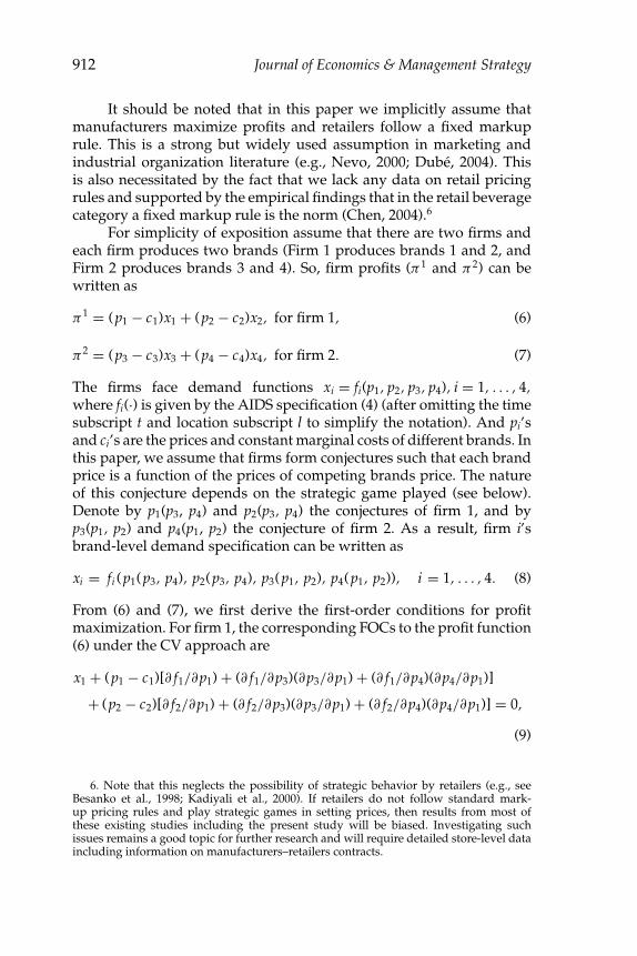
It should be noted that in this paper we implicitly assume thatmanufacturers maximize profits and retailers follow a fixed markuprule. This is a strong but widely used assumption in marketing andindustrial organization literature (e.g., Nevo, 2000; Dube, 2004). Thisis also necessitated by the fact that we lack any data on retail pricingrules and supported by the empirical findings that in the retail beveragecategory a fixed markup rule is the norm (Chen, 2004).6

For simplicity of exposition assume that there are two firms andeach firm produces two brands (Firm 1 produces brands 1 and 2, andFirm 2 produces brands 3 and 4). So, firm profits (π1 and π2) can bewritten as

π1 = (p1 − c1)x1 + (p2 − c2)x2, for firm 1, (6)

π2 = (p3 − c3)x3 + (p4 − c4)x4, for firm 2. (7)

The firms face demand functions xi = fi(p1, p2, p3, p4), i = 1, . . . , 4,where fi(·) is given by the AIDS specification (4) (after omitting the timesubscript t and location subscript l to simplify the notation). And pi’sand ci’s are the prices and constant marginal costs of different brands. Inthis paper, we assume that firms form conjectures such that each brandprice is a function of the prices of competing brands price. The natureof this conjecture depends on the strategic game played (see below).Denote by p1(p3, p4) and p2(p3, p4) the conjectures of firm 1, and byp3(p1, p2) and p4(p1, p2) the conjecture of firm 2. As a result, firm i’sbrand-level demand specification can be written as

xi = fi (p1(p3, p4), p2(p3, p4), p3(p1, p2), p4(p1, p2)), i = 1, . . . , 4. (8)

From (6) and (7), we first derive the first-order conditions for profitmaximization. For firm 1, the corresponding FOCs to the profit function(6) under the CV approach are

x1 + (p1 − c1)[∂ f1/∂p1) + (∂ f1/∂p3)(∂p3/∂p1) + (∂ f1/∂p4)(∂p4/∂p1)]

+ (p2 − c2)[∂ f2/∂p1) + (∂ f2/∂p3)(∂p3/∂p1) + (∂ f2/∂p4)(∂p4/∂p1)] = 0,

(9)

6. Note that this neglects the possibility of strategic behavior by retailers (e.g., seeBesanko et al., 1998; Kadiyali et al., 2000). If retailers do not follow standard mark-up pricing rules and play strategic games in setting prices, then results from most ofthese existing studies including the present study will be biased. Investigating suchissues remains a good topic for further research and will require detailed store-level dataincluding information on manufacturers–retailers contracts.


and

x2 + (p1 − c1)[∂ f1/∂p2) + (∂ f1/∂p3)(∂p3/∂p2) + (∂ f1/∂p4)(∂p4/∂p2)]

+ (p2 − c2)[∂ f2/∂p2) + (∂ f2/∂p3)(∂p3/∂p2) + (∂ f2/∂p4)(∂p4/∂p2)] = 0.

(10)

Similar first-order conditions can be derived for firm 2. Note that (9) and(10) can be alternatively expressed as

TR1 + (TR1 − TC1)ψ11 + (TR2 − TC2)ψ12 = 0, (11)

and

TR1 + (TR1 − TC1)ψ21 + (TR2 − TC2)ψ22 = 0, (12)

where TRi denotes revenue, TCi is total variable cost,ψ11 = [ε11 + ε13 η31×p1/p3 + ε14 η41 p1/p4], ψ12 = [ε21 + ε23 η31 p1/p3 + ε24 η41 p1/p4],)ψ21 =[ε12 + ε13 η32 p2/p3 + ε14 η42 p2/p4], ψ22 = [ε22 + ε23 η32 p2/p3 +ε24 η42 p2/p4], εij = ∂ln(f i)/∂ln(pj) is the price elasticity of demand,and ηij = ∂pi/∂pj is the brand j’s conjecture of brand i’s price response,i, j = 1, . . . , 4. Combining these results with similar results for firm 2gives

T R = (I + �)−1�TC, (13)

where TR = (TR1, TR2, TR3, TR4)′, TC = (TC1, TC2, TC3, TC4)′,

ψ =

�11 �12 0 0�21 �22 0 0

0 0 �33 �34

0 0 �43 �44

is a (4 × 4) matrix. Equation (13) provides a generic representation ofthe first-order conditions. This generic representation is similar to Nevo(1998). But, unlike Nevo and Cotterill et al., by transforming the FOCsin terms of elasticities, the supply side can be estimated with complexdemand specifications like AIDS or Translog.7

As mentioned earlier our derived FOCs are generic and differentstructures of ψ matrix correspond to different strategic games. For aNash–Bertrand game the ψ matrix becomes

7. Elasticites in AIDS can be specified as: Let µi = ∂wi∂ ln M = βi and µi j = ∂wi

∂ ln p j=

γi j − µi (α j + ∑k γ jk ln pk ). Then the expenditure elasticities are ei = µi

wi+ 1. The uncom-

pensated price elasticities are eui j = µi j

wi− δi j where δij is the Kronecker delta such that for

i = j δij = 1, else δij = 0.


�B =

ε11 ε21 0 0ε12 ε22 0 00 0 ε33 ε430 0 ε34 ε44

.

A comparison of ψ and ψB matrix indicates that the Nash–Bertrandgame restricts all ηij’s in the CV model to zero. So, the Nash–Bertrandgame is nested in our CV model.

Finally, note that a fully collusive game corresponds to the follow-ing ψ matrix:

�COL =

ε11 ε21 ε31 ε41ε12 ε22 ε32 ε42ε13 ε23 ε33 ε43ε14 ε24 ε34 ε44

.

Note that, when collusion is defined over all brands, then the (I + ψ)matrix becomes singular due to the Cournot aggregation condition fromdemand theory. In this paper, we do not investigate a fully collusivegame. Rather, we estimate partial brand-level collusion, such as col-lusive pricing between Coke and Pepsi with Sprite and Mountain Dewplaying a Bertrand game. Given the historic rivalries between Coca-ColaCompany and PepsiCo., strategic collusion in pricing is not realistic.Below, we estimate this collusive model mainly for the purpose of testingand comparing with other estimated models.

2.3 Reduced Form Expenditure Equation

Blundell and Robin (2000), and Dhar et al. (2003) found that expenditureM is endogenous, which has a significant impact on the parameterestimates.8 This suggests a need to control for endogeneity bias inthe model estimation. To do this, in a way similar to Blundell andRobin (2000), we specify a reduced-form expenditure equation wherehousehold expenditure in the lth city at time t is specified as a functionof median household income and a time trend,

Mlt = f (time trend, income). (14)

3. Model Selection Procedures

The analysis by GLV (1992) was one of the first to suggest proceduresto test appropriate strategic market models given probable alternative

8. In AIDS total expenditure is a function of price and quantity. As a result underlyingcauses of price endogeneity can also lead to endogeneity of expenditure variable.


cooperative and noncooperative games. They use both likelihood ratioand Wald tests to evaluate different model specifications. Of the twotypes of tests, the Wald test procedure is sensitive to functional formof the null hypothesis. In addition, the Wald test can only be used insituations where models are nested in each other. As such, GLV (1992)suggest estimating alternative models assuming different pure-strategygaming structures and then testing each model against the other usingnested and nonnested likelihood ratio tests.

In our view this is a suitable approach only in the case wherethe number of firms and products is small (preferably not more thantwo) and the demand and cost specification are not highly nonlinear.Otherwise as the number of products or firms increases, the numberof alternative models to be estimated also increases exponentially. Thisis due to the fact that a firm may play different strategies for differentbrands. One brand of the firm may be a Stackelberg leader but the otherbrand may have a price followship strategy.

It is even possible that firms may be collusive for some brandsand at the same time play noncollusive Stackelberg or Bertrand gameson other brands. For each brand, managers of Coca-Cola Company andPepsiCo. hypothetically can choose from four stylized pure strategies.These strategies are Stackelberg leadership, Stackelberg followship,noncooperative Bertrand, and collusion. For each brand, this impliesfour conceivable pure strategies in pricing against each of the competingbrands. In Table I, we diagrammatically present the strategy profilefor each brand. With four brands and four pure strategies in pricing,there are 256 (i.e., four firms with four strategies: 44) pure-strategyequilibria. Given the large numbers of pure-strategy games and highlynonlinear functional forms of our models, the use of likelihood ratio-based tests is not very attractive for our analysis. Indeed, we wouldneed to estimate 256 separate models to test each model against theother. Out-of-sample information may help us eliminate some of thegames.

In Table II, we present a sample of 12 representative games basedon pure-strategy pricing as described in Table I. Of all the probablegames, only the collusive game (1) is not nested in our CV model derivedearlier. Therefore, except for the collusive model, we can test games bytesting the statistical significance of the restrictions imposed by the gameon the estimated CV parameters.

We follow Dixit (1986) to develop null hypotheses in testing nestedmodels. Dixit (1986) shows that most pure strategy games can be nestedin a CV model. As a result the CV approach provides a parsimo-nious way of describing different pure strategy games. Following Dixit(1986), CV parameters can be interpreted as fixed points that establish


Tab

le

I.

Str

ate

gy

Pr

ofi

les

of

Each

Br

an

d

Peps

iM

ount

ain

Dew

Stac

kelb

erg

Stac

kelb

erg

Stac

kelb

erg

Stac

kelb

erg

Bra

ndL

ead

ersh

ipFo

llow

ship

Ber

tran

dC

ollu

sion

Lea

der

ship

Follo

wsh

ipB

ertr

and

Col

lusi

on

Cok

eSt

acke

lber

gL

ead

ersh

ip∗

∗St

acke

lber

gFo

llow

ship

∗∗

Ber

tran

d∗

∗C

ollu

sion

∗∗

Spri

teSt

acke

lber

gL

ead

ersh

ip∗

∗St

acke

lber

gFo

llow

ship

∗∗

Ber

tran

d∗

∗C

ollu

sion

∗∗

(∗)R

epre

sent

sbr

and

stra

tegi

esth

atar

ebe

ing

anal

yzed

inth

ispa

per.

Wit

hfo

urbr

and

s,no

teth

atth

eto

taln

umbe

rof

pure

stra

tegi

esth

atca

nbe

gene

rate

dis

256.


Table II.

Pure Strategy Games

Game Set 1: Game estimated and tested against CV model using likelihood ratio test:1 Collusive Game: Coke and Pepsi are the collusive brands. And Sprite and Mountain

Dew use Bertrand conjecture.2 Full Bertrand Game: Both the firms use Bertrand conjecture over all brands.

Game Set 2: To Test following strategic games we used Wald test procedure:3 Mixed Stackelberg and Bertrand Game 1: Coke leads Pepsi in a Stackelberg game. Rest

of the brand relationship is Bertrand.4 Mixed Stackelberg and Bertrand Game 2: Coke leads Mountain Dew in a Stackelberg

game. Rest of the brand relationship is Bertrand.5 Mixed Stackelberg and Bertrand Game 3: Coke leads both Pepsi and Mountain Dew in a

Stackelberg game. Rest of the brand relationship is Bertrand.6 Mixed Stackelberg and Bertrand Game 4: Coke leads Pepsi and Mountain Dew, and

Sprite leads Pepsi and Mountain Dew in a Stackelberg game.7 Mixed Stackelberg and Bertrand Game 5: Coke leads Pepsi and Mountain Dew leads

Sprite. Rest of the brand relationship is Bertrand.8 Mixed Stackelberg and Bertrand Game 7: Sprite leads Mountain Dew in a Stackelberg

game. Rest of the brand relationship is Bertrand.9 Mixed Stackelberg and Bertrand Game 9: Pepsi leads Coke in a Stackelberg game. Rest

of the brand relationship is Bertrand.10 Mixed Stackelberg and Bertrand Game 11: Pepsi leads Coke and Mountain Dew leads

Sprite in a Stackelberg game. Rest of the brand relationship is Bertrand.11 Mixed Stackelberg and Bertrand Game 15: Mountain Dew leads Sprite in a Stackelberg

game. Rest of the brand relationship is Bertrand.12 Mixed Stackelberg and Bertrand Game 15: Pepsi leads Coke and Sprite leads Mountain

Dew in a Stackelberg game. Rest of the brand relationship is Bertrand.

Note: This is the list of pure strategy pricing games analyzed in this paper.

consistency between the conjecture and the reaction function associatedwith a particular game. In this paper, we use our estimated CV modelto test different market structures presented in Table I. For example,if all the estimated CV parameters were zero, then the appropriategame in the market would be Bertrand (game 2 in Table II). This gen-erates the following null hypothesis (which can be tested using a Waldtest),

[ηC, P ηC, MD ηS, P ηS, MD ηP,C ηP, S ηMD, P ηMD, S]′ = [0]′

where C stands for Coke, P for Pepsi, S for Sprite and MD for MountainDew.

In the case of any Stackelberg game, Dixit (1986) has shown that atequilibrium, the conjectural variation parameter of a Stackelberg leadershould be equal to the slope of the reaction function of the follower,and followers’ CV parameter should be equal to zero. Thus, in a gamewhere Coca-Cola Company’s brands lead PepsiCo.’s brands (i.e., game


6 in Table II: both Coke and Sprite leads Pepsi and Mountain Dew),parametric restrictions generate the following null hypothesis:

[ηC, P ηC, MD ηS, P ηS, MD ηP,C ηP, S ηMD, P ηMD, S]′

= [RP,C RMD,C RP, S RMD, S 0 0 0 0]′,

where Ri,j’s are estimated slope of the reaction function of brand i of thefollower to a price change in j of the leader. For the rest of the games(as in Table II), we generate similar restrictions and test for them usinga Wald test. We estimate the slope of the reaction functions by totallydifferentiating the estimated first-order conditions, where in the case ofCoke’s reaction to Pepsi’s price change RC,P and RS,P can be stated as

RC, P =εC, P

pCpP

(TRC − TCC ) + εS, PpSpP

(TRS − TCS)

εC,C (TRC − TCC ) + εS,C (TRS − TCS) + TRC

RS, P =εC, P

pCpP

(TRC − TCC ) + εS, PpSpP

(TRS − TCS)

εS, S(TRS − TCS) + εC, S(TRC − TCC ) + TRS.

(15)

Similarly, we can derive the reaction function slopes for the rest of thebrands.

We propose a sequence of tests in the following manner. First, wetest our nonnested and partially nested models against each other usingthe Vuong test (1989). In the present paper, our collusive model andCV model are partially nested. One major advantage of the Vuong testis that it is directional. This implies that the test statistic not only tellsus whether the models are significantly different from each other butalso the sign of the test statistic indicates which model is appropriate.If we reject the collusive model, then the rest of the pure strategymodels can be tested using Wald tests because they are nested in our CVmodel.

4. Database

Table III provides brief descriptive statistics of all the variables usedin the analysis. Figure 1 plots the prices of the four brands. During theperiod of our study, Mountain Dew was consistently the most expensive,followed by Coke, Pepsi, and Sprite. Figure 2 plots volume sales bybrands. In terms of volume sales Coke and Pepsi were almost at thesame level, Sprite and Mountain Dew’s sales were significantly lowerthan Coke and Pepsi’s sales.


Table III.

Descriptive Statistics of Variables Used in theEconometric Analysis

Mean Purchase Characteristics

Price Expend. Volume Total($/gal) Share Per Unit Revenue Merchandizing (%)

Brands (pi) (wi) (VPUi) ($Million/city) (MCHi)

Coke 3.72 (0.09) 0.44 (0.12) 0.44 (0.07) 1.03 (0.93) 83.19 (7.53)Mt. Dew 3.93 (0.15) 0.05 (0.04) 0.44 (0.07) 0.09 (0.07) 69.22 (14.41)Pepsi 3.65 (0.09) 0.44 (0.13) 0.45 (0.07) 1.03 (0.95) 83.51 (7.66)Sprite 3.63 (0.09) 0.07 (0.02) 0.42 (0.05) 0.17 (0.15) 78.79 (9.75)

Mean Values of Other Explanatory Variables

Variables Units Mean

Median age (Demand Shift Variable − [Zlt]) Years 32.80 (2.4)

Median HH size (Demand Shift Variable − [Zlt]) No. 2.6 (0.1)% of HH less than $10k income (Demand Shift Variable − [Zlt]) % 16.8 (3.3)% of HH more than $50k income (Demand Shift Variable − [Zlt]) % 20.8 (4.9)Supermarket-to-grocery sales ratio (Demand Shift Variable − [Zlt]) % 78.9 (5.8)Concentration ratio (Price Function: CR4

lt) % 62.4 (13.8)Per capita expenditure (Mlt) $ 5.91 (1.22)Median income (Expenditure function: INClt) $ 28374 (3445.3)

Note: Numbers in parenthesis are the standard deviations.

5. Empirical Model Specification

As noted above, we modify the traditional AIDS specification withdemographic translating. As a result, our AIDS model incorporates aset of regional dummy variables along with selected socio-demographicvariables. Many previous studies using multi-market scanner data,including Cotterill (1994), Cotterill et al. (1996), and Hausman et al.(1994), use city-specific dummy variables to control for city-specificfixed effects for each brand. Here we control for regional differencesby including nine regional dummy variables.9

Our AIDS specification incorporates five demand shifters, Z,capturing the effects of demographics across marketing areas. Thesevariables are median household size, median household age, percentageof household earning less than $10,000, percentage of household earningmore the $50,000, and supermarket-to-grocery sales ratio. In addition,to maintain theoretical consistency of the AIDS model, the following

9. Our region definitions are based on census definition of divisions.


3.2

3.3

3.4

3.5

3.6

3.7

3.8

3.9

4

4.1

4.2

1 2 3 4 5 6 7 8

Price of SpritePrice of Coke Price of Pepsi Price of Mountain Dew

FIGURE 1. BRAND PRICE.

0

0.2

0.4

0.6

0.8

1

1.2

1 2 3 4 5 6 7 8

Time Period

Sal

es (

Mill

ion

s o

f G

allo

ns)

Sprite Pepsi Mountain DewCoke

FIGURE 2. VOLUME SALES BY BRANDS (MILLIONS OF GALLONS).

restrictions based on (5) are applied to the demographic-translatingparameter α0i,

α0i = dir Dr , dir = 1, i = 1, . . . , N. (16)

where dir is the parameter for the ith brand associated with the regionaldummy variable Dr for the rth region. Note that as a result, our demandequations do not have intercept terms. We assume a constant linear


marginal cost specification. Such cost specification is quite common andperforms reasonably well in structural market analysis (e.g., GLV, 1992;Kadiyali et al., 1996; Cotterill et al., 2000). The total cost function is

T Costilt = Ui + MCostilt × xilt, (17)

where Ui is the brand-specific unobservable (by the econometrician)cost component and assumed not to vary at the mean of the variables.MCostilt is the observable cost component and we specify it as

MCostilt = θi1U PVilt + θi2 MC Hilt, (18)

where UPVilt is the unit per volume of the ith product in the lth cityat time t and represents the average size of the purchase. For example,if a consumer purchases only one-gallon bottles of a brand, then unitper volume for that brand is one. Alternatively, if this consumer buys ahalf-gallon bottle then the unit per volume is 2. This variable capturespackaging-related cost variations, as smaller package size per volumeimplies higher costs to produce, to distribute, and to shelve. The variableMCHilt measures percentage of a CSD brand i sold in a city l with anytype of merchandising (e.g., buy one get one free, cross promotionswith other products, etc.). This variable captures merchandising costsof selling a brand. For example, if a brand is sold through promotionsuch as: “buy one get one free,” then the cost of providing the secondunit will be reflected in this variable.

Following Blundell and Robin (2000), to control for expenditureendogeneity, the reduced form expenditure function in (14) is specifiedas

Mlt = Trendt +9∑

r=1

δr Dr + φ1INClt + φ2INC2lt, t = 1, . . . , 8, (19)

where Trendt in (19) is a linear trend, capturing any time-specific unob-servable effect on consumer soft drink expenditure. The variables Dr’sare the regional dummy variables defined above and capture region-specific variations in per capita expenditure. The variable INClt is themedian household income in city l and is used to capture the effect ofincome differences on CSD purchases.

We estimate the system of three demand and four FOCs usingFIML estimation procedure under normality.10 One demand equation

10. Although the demand specification involves budget shares, note that the consump-tion data used in our empirical analysis do not involve censored observations (i.e., theobserved budget shares remain away from the boundaries of their feasible values). In thiscontext, estimating the model under normality assumption does not appear unreasonableand it provides an empirically tractable way of estimating a highly nonlinear model whiledealing with prevalent endogeneity issues.


drops out due to aggregation restrictions of AIDS. The variance–covariance matrix and the parameter vector are estimated by specifyingthe concentrated log-likelihood function of the system. The Jacobian ofthe concentrated log-likelihood function is derived based on the modelswith eight endogenous variables: 3 quantity-demanded variables (e.g.,xi’s), 4 price variables (e.g., pi’s), and the expenditure variable (e.g.,M). Note that in the process of estimation, we have one less quantity-demanded variable than price variables. This is due to the AIDS shareequation adding-up condition. Because the sum of the brand shares is 1;one needs only estimate three share equations to obtain the parameterestimates of the fourth. We can express the demand for the fourth brandas a function of other endogenous variables, x4 = M − (p1x1 + p2x2 +p3x3)/p4.

6. Regression Results and Testof Alternative Models

We estimate three alternative models: (1) collusive oligopoly where thetwo firms collude on the price of Coke and Pepsi, (2) the Bertrand model,and (3) the conjectural variation model.11

We assume that the demand shifters and the variables in the costand expenditure specification are exogenous. In general, the reduced-form specifications (i.e., equations (17) and (18)) are always identified.The issue of parameter identification in nonlinear structural model israther complex.12 We checked the order condition for identificationthat would apply to a linearized version of the demand equation (4)and found it to be satisfied. Finally, we did not uncover numericaldifficulties in implementing the FIML estimation and our estimatedresults are robust to the iterative process of estimation. As pointed outby Mittelhammer et al. (2000, pp. 474–475) in nonlinear full informationmaximum likelihood estimation, we interpret this as evidence that eachof the demand equations is identified.

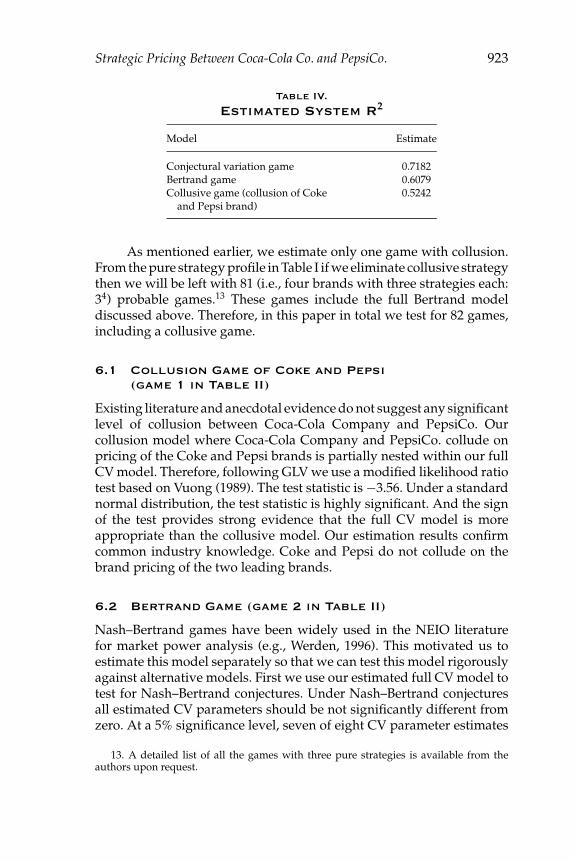
Table IV presents system R2 based on McElroy (1977). In termsof goodness of fit the full CV model fits the best and collusive modelgives the poorest fit. However, goodness-of-fit measure in nonlinearregression may not be the appropriate tool to choose among models. Totest for an appropriate nesting structure and to select the best model werun further tests based on likelihood ratio and Wald test statistics.

11. Detailed regression results of the estimated models are available from the authorsupon request.

12. For a detailed discussion please refer to Mittelhammer et al. (2000, pp. 474–475).


Table IV.

Estimated System R2

Model Estimate

Conjectural variation game 0.7182Bertrand game 0.6079Collusive game (collusion of Coke 0.5242

and Pepsi brand)

As mentioned earlier, we estimate only one game with collusion.From the pure strategy profile in Table I if we eliminate collusive strategythen we will be left with 81 (i.e., four brands with three strategies each:34) probable games.13 These games include the full Bertrand modeldiscussed above. Therefore, in this paper in total we test for 82 games,including a collusive game.

6.1 Collusion Game of Coke and Pepsi(game 1 in Table II)

Existing literature and anecdotal evidence do not suggest any significantlevel of collusion between Coca-Cola Company and PepsiCo. Ourcollusion model where Coca-Cola Company and PepsiCo. collude onpricing of the Coke and Pepsi brands is partially nested within our fullCV model. Therefore, following GLV we use a modified likelihood ratiotest based on Vuong (1989). The test statistic is −3.56. Under a standardnormal distribution, the test statistic is highly significant. And the signof the test provides strong evidence that the full CV model is moreappropriate than the collusive model. Our estimation results confirmcommon industry knowledge. Coke and Pepsi do not collude on thebrand pricing of the two leading brands.

6.2 Bertrand Game (game 2 in Table II)

Nash–Bertrand games have been widely used in the NEIO literaturefor market power analysis (e.g., Werden, 1996). This motivated us toestimate this model separately so that we can test this model rigorouslyagainst alternative models. First we use our estimated full CV model totest for Nash–Bertrand conjectures. Under Nash–Bertrand conjecturesall estimated CV parameters should be not significantly different fromzero. At a 5% significance level, seven of eight CV parameter estimates

13. A detailed list of all the games with three pure strategies is available from theauthors upon request.


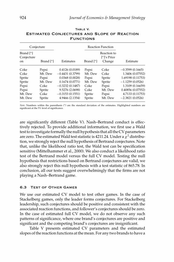
Table V.

Estimated Conjectures and Slope of ReactionFunctions

Conjecture Reaction Function

Brand [∗] Reaction toConjecture [∗]’s Priceon Brand [∗] Estimates Brand [∗] Change Estimate

Coke Pepsi 0.4126 (0.0189) Pepsi Coke −0.3599 (0.1665)Coke Mt. Dew −0.4431 (0.3799) Mt. Dew Coke 1.3406 (0.07552)Sprite Pepsi 0.0368 (0.0028) Pepsi Sprite 1.69198 (0.11753)Sprite Mt. Dew 0.1674 (0.0771) Mt. Dew Sprite −1.1259 (0.0526)Pepsi Coke −0.3232 (0.1487) Coke Pepsi 1.3109 (0.16659)Pepsi Sprite 9.5276 (2.0698) Coke Mt. Dew 0.40856 (0.07552)Mt. Dew Coke −0.3153 (0.1551) Sprite Pepsi 4.7133 (0.11753)Mt. Dew Sprite 4.9466 (2.1354) Sprite Mt. Dew −2.3821 (0.0526)

Note: Numbers within the parenthesis (∗) are the standard deviation of the estimates. Highlighted numbers aresignificant at the 5% level of significance.

are significantly different (Table V). Nash–Bertrand conduct is effec-tively rejected. To provide additional information, we first use a Waldtest to investigate formally the null hypothesis that all the CV parametersare zero. The estimated Wald test statistic is 4211.24. Under a χ2 distribu-tion, we strongly reject the null hypothesis of Bertrand conjectures. Notethat, unlike the likelihood ratio test, the Wald test can be specificationsensitive (Mittelhammer et al., 2000). We also conduct a likelihood ratiotest of the Bertrand model versus the full CV model. Testing the nullhypothesis that restrictions based on Bertrand conjectures are valid, wealso strongly reject this null hypothesis with a test statistic of 865.78. Inconclusion, all our tests suggest overwhelmingly that the firms are notplaying a Nash–Bertrand game.

6.3 Test of Other Games

We use our estimated CV model to test other games. In the case ofStackelberg games, only the leader forms conjectures. For Stackelbergleadership, such conjectures should be positive and consistent with theassociated reaction functions, and follower’s conjectures should be zero.In the case of estimated full CV model, we do not observe any suchpatterns of significance, where one brand’s conjectures are positive andsignificant and the competing brand’s conjectures are insignificant.

Table V presents estimated CV parameters and the estimatedslopes of the reaction functions at the mean. For any two brands to have a


Stackelberg leader–follower relationship, the estimated CV parametersof the leader should be equal to the estimated reaction slope of thefollower. For example, for Coke to be the Stackelberg leader over Pepsi,Coke’s estimated conjecture over Pepsi’s price (i.e., 0.41) should be equalto the estimated reaction function slope of Pepsi (i.e., −0.36). In addition,Pepsi’s conjecture on Coke’s price (i.e., −0.32) should be equal to zero.Assuming that other brand relationships are Bertrand our Wald test ofthe game investigates the empirical validity of these restrictions. Theother games are tested in a similar fashion, using the restrictions on CVestimates and estimated reaction function slopes. We reject all the gamesat the 5% level of significance.14 Using the Wald test, we fail to acceptany of the other probable games.15

6.4 Consistency of Conjectures

We failed to accept any of the game with Stackelberg equilibrium. There-fore, we test for a less restrictive condition of Stackelberg leadership.

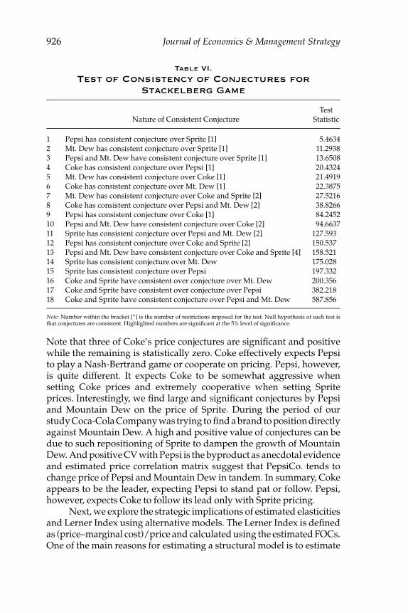
That is, we test for consistency of estimated conjectures. Consis-tency of conjectures implies that a firm behaves as if it is a Stackelbergleader even though there may not be any firm behaving as a Stackelbergfollower. Results of the test of consistent conjectures are presentedin Table VI. In general, our estimated reaction function slopes at themean are quite different from the corresponding conjectures. This helpsexplain the overwhelming rejection of all the game scenarios withStackelberg conjectures. Only Pepsi has a consistent conjecture withrespect to Sprite at a 1% level of significance. One is left to the conclusionthat the actual games being played are more complex than the relativelysimple oligopoly games explained in the textbooks.

Failure to accept any specific nested games implies that the CVmodel is the most appropriate and general model. Of the estimatedconjectures only one is insignificant and three out of eight estimatedconjectures are negative. Interestingly, we find asymmetric price con-jectures between the Coke and Pepsi brands. Coke has a positive priceconjecture (0.4126) for Pepsi’s price but Pepsi’s conjecture for Coke’sprice (−0.3232) is negative. In terms of market conducts, this suggeststhat Coke, the market leader, would like to play a cooperative game,that is, expects Pepsi to follow its pricing. Pepsi, however, is pessimisticand expects rivalry from Coke, that is, it expects Coke to cut price whenit increases price. In Table V, however, one observes a more generalpattern of strategic interaction between the two soft drink companies.

14. Detail test procedures and statistics are available from the authors upon request.15. A list of probable games and detailed test statistics of all the games tested is

available from the authors on request.


Table VI.

Test of Consistency of Conjectures forStackelberg Game

TestNature of Consistent Conjecture Statistic

1 Pepsi has consistent conjecture over Sprite [1] 5.46342 Mt. Dew has consistent conjecture over Sprite [1] 11.29383 Pepsi and Mt. Dew have consistent conjecture over Sprite [1] 13.65084 Coke has consistent conjecture over Pepsi [1] 20.43245 Mt. Dew has consistent conjecture over Coke [1] 21.49196 Coke has consistent conjecture over Mt. Dew [1] 22.38757 Mt. Dew has consistent conjecture over Coke and Sprite [2] 27.52168 Coke has consistent conjecture over Pepsi and Mt. Dew [2] 38.82669 Pepsi has consistent conjecture over Coke [1] 84.245210 Pepsi and Mt. Dew have consistent conjecture over Coke [2] 94.663711 Sprite has consistent conjecture over Pepsi and Mt. Dew [2] 127.59312 Pepsi has consistent conjecture over Coke and Sprite [2] 150.53713 Pepsi and Mt. Dew have consistent conjecture over Coke and Sprite [4] 158.52114 Sprite has consistent conjecture over Mt. Dew 175.02815 Sprite has consistent conjecture over Pepsi 197.33216 Coke and Sprite have consistent over conjecture over Mt. Dew 200.35617 Coke and Sprite have consistent over conjecture over Pepsi 382.21818 Coke and Sprite have consistent conjecture over Pepsi and Mt. Dew 587.856

Note: Number within the bracket [∗] is the number of restrictions imposed for the test. Null hypothesis of each test isthat conjectures are consistent. Highlighted numbers are significant at the 5% level of significance.

Note that three of Coke’s price conjectures are significant and positivewhile the remaining is statistically zero. Coke effectively expects Pepsito play a Nash-Bertrand game or cooperate on pricing. Pepsi, however,is quite different. It expects Coke to be somewhat aggressive whensetting Coke prices and extremely cooperative when setting Spriteprices. Interestingly, we find large and significant conjectures by Pepsiand Mountain Dew on the price of Sprite. During the period of ourstudy Coca-Cola Company was trying to find a brand to position directlyagainst Mountain Dew. A high and positive value of conjectures can bedue to such repositioning of Sprite to dampen the growth of MountainDew. And positive CV with Pepsi is the byproduct as anecdotal evidenceand estimated price correlation matrix suggest that PepsiCo. tends tochange price of Pepsi and Mountain Dew in tandem. In summary, Cokeappears to be the leader, expecting Pepsi to stand pat or follow. Pepsi,however, expects Coke to follow its lead only with Sprite pricing.

Next, we explore the strategic implications of estimated elasticitiesand Lerner Index using alternative models. The Lerner Index is definedas (price–marginal cost)/price and calculated using the estimated FOCs.One of the main reasons for estimating a structural model is to estimate


Table VII.

Price Elasticity Matrix (CV Model)

Coke Sprite Pepsi Mountain Dew

Coke −3.7948 (0.0591) 0.0016 (0.0051) 2.1814 (0.0538) 0.4311 (0.0108)Sprite 0.1468 (0.0426) −2.8400 (0.0707) 3.6776 (0.1242) −1.8568 (0.0562)Pepsi 2.3381 (0.0602) 0.5995 (0.0177) −3.9384 (0.0583) 0.2529 (0.0108)Mountain Dew 3.5060 (0.1468) −2.7280 (0.0831) 1.7659 (0.1082) −4.3877 (0.0734)

Notes: Numbers within the parenthesis (∗) are the standard deviation of the estimates. Rows reflect percentage changein demand and column reflect percentage change in price. Highlighted numbers are significant at the 5% level ofsignificance.

Table VIII.

Expenditure ElasticityMatrix (CV Model)

Brands Estimate

Coke 1.1806 (0.0282)Sprite 0.8725 (0.0773)Pepsi 0.7478 (0.0340)Mountain Dew 1.8438 (0.2102)

Note: Numbers within the parenthesis (∗) are the standard deviationof the estimates. Highlighted numbers are significant at the 5% levelof significance.

price and expenditure elasticities, and associated indicators of marketpower (e.g., Lerner Index). We evaluate the impact of alternative modelspecifications on elasticity and market power estimates. Tables VII andVIII present price and expenditure elasticity estimates for the full CVmodel.

Dhar et al. (2003) and Villas-Boas and Winer (1999) found thatafter controlling price and expenditure endogeneity, the efficiency ofthe elasticity estimates improves dramatically. This study also findssignificant improvements in terms of the efficiency of our elasticityestimates.16

In our CV model, the estimated own-price elasticities have theanticipated signs, and own- and cross-price elasticities satisfy all thebasic utility theory restrictions (namely symmetry, Cournot, and Engelaggregation). In addition, all the estimated cross- and own-price elastici-ties are highly significant suggesting rich strategic relationships betweenbrands. Our estimated expenditure elasticities are all positive and vary

16. Detailed results of models without controlling for endogeneity are available fromthe authors upon request.


Table IX.

Lerner Index

Estimate

Strategic Game Coke Sprite Pepsi Mountain Dew

Conjectural variation game [1] 0.3233 0.3795 0.3221 0.5197Bertrand game [2] 0.2647 0.2991 0.2601 0.4625Collusive game [5] 0.7274 0.1940 0.6726 0.6325

between 0.74 and 1.85, with Pepsi being the most inelastic and MountainDew being the most elastic brand. Interestingly, our elasticity estimatessuggest that Mountain Dew and Sprite behave as complements. Asmentioned before Mountain Dew is unique in the CSD market. In termsof taste it is similar to Sprite but on the other hand, in terms of caffeinecontent, it is positioned closer to Coke. It is probable that consumerswith preference for lemon/lime-flavored drink use Mountain Dew as acomplement to Sprite due to its caffeine content. In a study of the CSDmarket, Dube (2004) also found that consumers tend to treat caffeineand non-caffeine CSD drinks as complements.

Table IX presents Lerner indices. Each is an estimate of price–costmargin for the entire soft drink marketing channel, that is, it includesmargins of the manufacturers, distributors, and retailers. Using our CVmodel, Pepsi has the lowest price–cost margin and Mountain Dew hasthe highest. This is consistent with the fact that Mountain Dew is thefastest growing carbonated soft drink brand, with a higher reportedprofit margin than most brands.17

For the purpose of evaluating the impact of model specification, wealso estimate the Lerner Index for the Bertrand and collusive games. Inaddition, note that Lerner Indices based on our CV model are higher thanin the case of the Bertrand game. This is due to the fact that our estimatedCV parameters are predominantly positive leading to higher markupsfor all the brands. To compare the three games, we calculated the averageabsolute percentage differences (APD) among the estimated LernerIndices, where APD between any two estimates (ε∗ and ε∗∗) is defined as

APD = {100 |ε∗ − ε∗∗|}/{0.5 |ε∗ + ε∗∗|}.The average APD between Lerner Index estimates from the CV and thefull Bertrand game is 19.14. Between the CV and the collusive model

17. According to Andrew Conway, a beverage analyst for Morgan Stanley & Company:“Mountain Dew gives PepsiCo. about 20% of its profits because it’s heavily skewed towardthe high-profit vending-machine and convenience markets. In these channels, MountainDew is rarely sold at a discount” (New York Times, Dec 16, 1996).


it is 57.92. Such large differences in an estimated Lerner Index acrossmodels indicate that appropriate model specification is important forempirical market power analysis.

7. Concluding Remarks

In this paper, we analyze the strategic behavior of Coca-Cola Companyand PepsiCo. in the carbonated soft drink market. This is the first studyto use the flexible nonlinear AIDS model within a structural econometricmodel of firm (brand) conduct. In addition, we derive generic first-orderconditions under different profit-maximizing scenarios that can be usedwith most demand specifications and to test for strategic games. Thisapproach avoids linear approximation of the demand and/or first-orderconditions.

In this paper, we test for brand-level alternative games betweenfirms. Most of the earlier studies in differentiated product oligopolyeither tested for games at the aggregate level (i.e., Cotterill et al., 2000)or between two brands (Golan et al., 2000; and GLV, 1992). Given thatmost oligopolistic firms produce different brands, test of brand-levelstrategic competition is more realistic.

We first test a partially nested collusive model against a CV model.We find statistical evidence that the CV model is more appropriate thanthe collusive model. The remaining stylized games considered in thispaper are in fact nested in the CV model. Our tests for specific stylizedmulti-brand multifirm market pure strategy models (relying on Waldtests) are attractive because of their simplicity. Treating each game as anull hypothesis, we reject all the null hypotheses. Our overall test resultsimply that the pricing game being played in this market is much morecomplex than the stylized games being tested.

It may well be that some complex game not considered in thispaper conforms to the estimated CV model. As a result, if a researcherdoes not have out-of-sample information on the specific game beingplayed then it is appropriate to estimate a CV model.

We use estimated parameters from different models to estimateelasticities and the Lerner Index. We find these estimates to be quitesensitive to model specifications. The empirical evidence suggests thatthe CV model is the most appropriate.

One of the shortcomings of this paper is that we do not considermixed strategy games as in Golan et al. (2000). The pure strategy gamesconsidered here are degenerate mixed strategy games. It is possible thatthe actual game played is a game with mixed strategies. Additionalresearch is needed to consider such models with flexible demandspecification such as AIDS.


References

Bajari, P. and C.L. Benkard, March 2003, “Discrete Choice of Models as Structural Modelsof Demand: Some Economic Implications of Common Approaches,” Working Paper,Department of Economics, Stanford University.

Berry, S.T.,1994, “Estimating Discrete-Choice Models of Product Differentiation,” RandJournal of Economics, 25, 242–262.

Besanko, D., S. Gupta, and D. Jain, 1998, “Logit Demand Estimation under CompetitivePricing behavior: An Equilibrium Framework,” Management Science, 44, 1533–1547.

Blundell, R. and J.M. Robin, 2000, “Latent Separability: Grouping Goods without WeakSeparability,” Econometrica, 68, 53–84.

Brander, J.A. and A. Zhang, 1990, “Market Conduct in the Airline Industry: An EmpiricalInvestigation,” Rand Journal of Economics, 21, 567–583.

Brand, J.A. and B.J. Spancer, 1985, “Tacit Collusion, Free Entry, and Welfare,” Journal ofIndustrial Economics, 33, 277–294.

Chen, X., 2004, “Assessing The Role of Strategic and Efficiency Factor in a Channel Switch,”Working paper, Carlson School of Management, University of Minnesota.

Cotterill, R.W., 1994, “An Econometric Analysis of the Demand for RTE Cereal: ProductMarket Definition and Unilateral Market Power Effects,” Exhibit C in Affidavit ofR.W. Cotterill, 9/6/1994, State of New York v Kraft General Foods et al., 93 civ 0811.(reprinted as University of Connecticut Food Marketing Policy Center Research ReportNo. 35.

Cotterill, R.W., A.W. Franklin, and L.Y. Ma, 1996, “Measuring Market Power Effects inDifferentiated Product Industries: An Application to the Soft Drink Industry,” ResearchReport, Storrs, CT: Food Marketing Policy Center, University of Connecticut.

Cotterill, R.W. and W.P. Putsis, Jr., 2001, “Testing the Theory: Assumptions on VerticalStrategic Interaction and Demand Functional Form,” Journal of Retailing, 77, 83–109.

Cotterill, R.W., W.P. Putsis, Jr., and R. Dhar, 2000, “Assessing the Competitive Interactionbetween Private Labels and National Brands,” Journal of Business, 73, 109–137.

Deaton, A.S. and J. Muellbauer, 1980a, Economics and Consumer Behavior, New York:Cambridge University Press.

—– and —–, June 1980b, “An Almost Ideal Demand System,” American Economic Review,70, 312–326.

Dhar, T., J.P. Chavas, and B.W. Gould, 2003, “An Empirical Assessment of Endogeneity Is-sues in Demand Analysis for Differentiated Products,” American Journal of AgriculturalEconomics, 85, 605–617.

Dixit, A., 1986, “Comparative Statics for Oligopoly,” International Economic Review, 27,107–122.

Dixon, H.D. and E. Somma, 2003, “The Evolution of Consistent Conjectures,” Journal ofEconomic Behavior and Organization, 51, 523–536.

Dube, J.P., 2004, “Multiple Discreteness and Product Differentiation: Demand for Carbon-ated Soft Drinks,” Marketing Science, 23(1), 66–81.

Friedman, J.W. and C. Mezzetti, 2002, “Bounded Rationality, Dynamic Oligopoly, andConjectural Variations,” Journal of Economic Behavior and Organization, 4, 287–306.

Gasmi, F., J.J. Laffont, and Q. Vuong, 1992, “Econometric Analysis of Collusive Behaviorin a Soft-Drink Market,” Journal of Economics and Management Strategy, 1(2), 277–311.

Genesove, D. and W.P. Mullin, 1998, “Testing Static Oligopoly Models: Conduct and Costin the Sugar Industry, 1890–1914,” The Rand Journal of Economics, 29(2), 355–377.

Golan, A., L.S. Karp, and J.M. Perloff, 2000, “Estimating Coke and Pepsi’s Price andAdvertising Strategies,” Journal of Business & Economic Statistics, 18(4), 398–409.


Hausman, J., 1997, “Valuation of New Goods Under Perfect and Imperfect Competition,”in T. Bresnahan and R. Gordon (eds.), The Economics of New Goods, Chicago: Universityof Chicago Press.

Hausman, J., G. Leonard, and J.D. Zona, 1994, “Competitive Analysis with DifferentiatedProducts,” Annales D’Economie et de Statistique, 34, 159–180.

Kadiyali, V., P. Chintagunta, and N. Vilcassim, 2000, “Manufacturer-Retailer ChannelInteractions and Implications for Channel Power: An Empirical Investigation of Pricingin a Local Market,” Marketing Science, 19, 127–148.

—–, N.J. Vilcassim, and P.K. Chintagunta, 1996, “Empirical Analysis of CompetitiveProduct Line Pricing Decisions: Lead, Follow, or Move Together?” Journal of Business,69, 459–487.

McElroy, M., 1977, “Goodness of Fit for Seemingly Unrelated Regressions: Glahn’s R2yx

and Hooper’s r2,” Journal of Econometrics, 6, 381–387.Mittelhammer, R.C., G.G. Judge, and D.J. Miller, 2000, Econometric Foundations, 1st ed.,

Cambridge, UK: Cambridge University Press.Moschini, G., D. Moro, and R.D. Green, 1994, “Maintaining and Testing Separability in

Demand Systems,” American Journal of Agricultural Economics, 76, 61–73.Nevo, A., 1998, “Identification of the Oligopoly Solution Concept in a Differentiated-

Products Industry,” Economics Letters, 59(3), 391–395.—–, 2000, “Mergers with Differentiated Products: The Case of the Ready-to-Eat Cereal

Industry,” RAND Journal of Economics, 31, 395–421.—–, 2001, “Measuring Market Power in the Ready-to-Eat Cereal Industry,” Econometrica,

69, 307–342.Tirole, J., 1988, The Theory of Industrial Organization, Cambridge, MA: MIT Press.Villas-Boas, J.M. and R. Winer, 1999, “Endogeneity in Brand Choice Model,” Management

Science, 45, 1324–1338.Villas-Boas, J.M. and Y. Zhao, 2005, “Retailer, Manufacturers and Individual Consumers:

Modeling the Supply Side of the Ketchup Marketplace,” Journal of Marketing Research,42, 83–95.

Vuong, Q.H., 1989, “Likelihood Ratio Tests for Model Selection and Non-nested Hypothe-ses,” Econometrica, 57(2), 307–333.

Werden, G., 1996, “Demand Elasticities in Antitrust Analysis,” Economic Analysis GroupDiscussion Paper, USDOJ, EAG 96-11 (November 1996).

An Econometric Analysis of Brand-Level Strategic Pricing Between ...

Documents

Transcript of An Econometric Analysis of Brand-Level Strategic Pricing Between ...