An Autonomous Excavator with Vision-Based Track Slippage ...psaeedi/cst_2005.pdf · An Autonomous...
18
1 An Autonomous Excavator with Vision-Based Track Slippage Control Parvaneh Saeedi, Peter D. Lawrence, David G. Lowe, Poul Jacobsen, Dejan Kusalovic, Kevin Ardron, and Paul H. Sorensen Abstract— This paper describes a vision-based control system for a tracked mobile robot (an excavator). The system includes several controllers that collaborate to move the mobile vehicle from a starting position to a goal position. First, the path planner designs an optimum path using a predefined elevation map of the work space. Second, a fuzzy logic path-tracking controller estimates the rotational and translational velocities for the vehicle to move along the pre-designed path. Third, a cross-coupling controller corrects the possible orientation error that may occur when moving along the path. A motor controller then converts the track velocities to the corresponding rotational wheel velocities. Fourth, a vision-based motion tracking system is implemented to find the 3D motion of the vehicle as it moves in the work space. Finally, a specially-designed slippage controller detects slippage by comparing the motion through reading of flowmeters and the vision system. If slippage has occurred, the remaining path is corrected within the path tracking controller to stop at the goal position. Experiments are conducted to test and verify the presented control system. An analysis of the results shows that improvement is achieved in both path-tracking accuracy and slippage control problems. Index Terms— Robot vision, visual motion control, trajectory control, path planner, track slippage, vehicle position sensing, excavator control, motor control, vision-based trajectory estima- tion. I. I NTRODUCTION T RACKED vehicles, such as excavator-type machines, are widely used in industries such as forestry, construction and mining. These machines are used for a variety of tasks, such as lifting and carrying loads, digging and ground level- ing. Autonomous controls for driving or assisting humans in operating these machines can potentially improve the opera- tional safety and efficiency. Much research has gone toward controlling vehicle movement to reduce human interaction when the vehicle is performing a task [1] [2]. Removing the operator for direct control of the machine has been achieved in teleoperation [3] [4] [5]. Achieving this goal in natural environments requires planning every movement, to avoid any obstacles and to locate the vehicle at each time with respect to a global coordinate system. With the application of an effective control scheme, human error can be minimized or completely removed, and more consistent operation of the vehicle can be achieved to increase efficiency. Many methods for outdoor path planning have been de- veloped to find feasible paths from start to end loca- tions [6] [7] [8]. Some of these methods rely on a prior map of the environment, to be provided by an operator. Since a static map is not sufficient, due to outdoor changes, other methods use sensory devices such as laser range finders and stereo cameras to create and update their own neighborhood maps as the vehicle navigates. Numerous methods have also been developed to track tra- jectories and paths outdoors [9]–[15]. Some of these methods implement non-linear trajectory control algorithms using the difference between the actual and virtual reference positions. Others accomplish the task by generating error vectors from the lateral displacement and heading errors. Path tracking has also been performed using feedforward compensation for the steering mechanism to provide anticipatory control of the steering lag. Many sensors have been developed and applied to robot localization. Wheel sensors such as encoders and resolvers suffer from wheel-slip. Estimating position using angular rate sensors and accelerometers suffers from integration error due to the effects of noise. Sonar, a low resolution system, is sensitive to environmental disturbances (wind, temperature, foliage motion and machine noises), Laser range scanning is expensive and has a low image update rate. Even GPS, can suffer from occlusion of line-of-sight to satellites, low accuracy, and low update rate. Since solid-state cameras and computers are rapidly improving in quality and speed driven by a consumer market, they are an tempting platform on which to build a robot localization system. The main long-term goal of this work is to move a tracked vehicle from a starting point to a target point in an unstructured outdoor environment. This paper describes the design and implementation of a complete system for a Takeuchi TB035 excavator that contains all of the subsystems necessary for this task. In particular, path planning, path tracking control, excavator track control, and visual motion tracking were selected as necessary building blocks. To make the overall development feasible in a reasonable time and to allow for real-time performance, some constraints were applied. The system was constrained to plan and execute straight line segments and small-radius turns, and that the vision system would be angled down to avoid sun, and thus be protected from raindrop accumulation - limiting the scene to a local region only. A unique aspect of this work, enabled by the vision system, is to detect and correct track slippage. Excessive track slippage can take place on slopes in various ground conditions, and can lead to soil erosion. The proposed path planner can be tuned to find paths that will reduce the possibilities of excessive slippage. II. MOTION CONTROL SYSTEM OVERVIEW A block diagram of the semi-autonomous vehicle motion control system is shown in Figure 1. The human operator
Transcript of An Autonomous Excavator with Vision-Based Track Slippage ...psaeedi/cst_2005.pdf · An Autonomous...
1
An Autonomous Excavator with Vision-BasedTrack Slippage Control
Parvaneh Saeedi, Peter D. Lawrence, David G. Lowe, Poul Jacobsen, Dejan Kusalovic, Kevin Ardron,and Paul H. Sorensen
Abstract— This paper describes a vision-based control systemfor a tracked mobile robot (an excavator). The system includesseveral controllers that collaborate to move the mobile vehiclefrom a starting position to a goal position. First, the path plannerdesigns an optimum path using a predefined elevation map ofthe work space. Second, a fuzzy logic path-tracking controllerestimates the rotational and translational velocities for the vehicleto move along the pre-designed path. Third, a cross-couplingcontroller corrects the possible orientation error that may occurwhen moving along the path. A motor controller then converts thetrack velocities to the corresponding rotational wheel velocities.Fourth, a vision-based motion tracking system is implemented tofind the 3D motion of the vehicle as it moves in the work space.Finally, a specially-designed slippage controller detects slippageby comparing the motion through reading of flowmeters andthe vision system. If slippage has occurred, the remaining pathis corrected within the path tracking controller to stop at thegoal position. Experiments are conducted to test and verify thepresented control system. An analysis of the results shows thatimprovement is achieved in both path-tracking accuracy andslippage control problems.
Index Terms— Robot vision, visual motion control, trajectorycontrol, path planner, track slippage, vehicle position sensing,excavator control, motor control, vision-based trajectory estima-tion.
I. INTRODUCTION
TRACKED vehicles, such as excavator-type machines, arewidely used in industries such as forestry, construction
and mining. These machines are used for a variety of tasks,such as lifting and carrying loads, digging and ground level-ing. Autonomous controls for driving or assisting humans inoperating these machines can potentially improve the opera-tional safety and efficiency. Much research has gone towardcontrolling vehicle movement to reduce human interactionwhen the vehicle is performing a task [1] [2]. Removing theoperator for direct control of the machine has been achievedin teleoperation [3] [4] [5]. Achieving this goal in naturalenvironments requires planning every movement, to avoid anyobstacles and to locate the vehicle at each time with respect toa global coordinate system. With the application of an effectivecontrol scheme, human error can be minimized or completelyremoved, and more consistent operation of the vehicle can beachieved to increase efficiency.
Many methods for outdoor path planning have been de-veloped to find feasible paths from start to end loca-tions [6] [7] [8]. Some of these methods rely on a prior map ofthe environment, to be provided by an operator. Since a staticmap is not sufficient, due to outdoor changes, other methodsuse sensory devices such as laser range finders and stereo
cameras to create and update their own neighborhood mapsas the vehicle navigates.
Numerous methods have also been developed to track tra-jectories and paths outdoors [9]–[15]. Some of these methodsimplement non-linear trajectory control algorithms using thedifference between the actual and virtual reference positions.Others accomplish the task by generating error vectors fromthe lateral displacement and heading errors. Path trackinghas also been performed using feedforward compensation forthe steering mechanism to provide anticipatory control of thesteering lag.
Many sensors have been developed and applied to robotlocalization. Wheel sensors such as encoders and resolverssuffer from wheel-slip. Estimating position using angular ratesensors and accelerometers suffers from integration error dueto the effects of noise. Sonar, a low resolution system, issensitive to environmental disturbances (wind, temperature,foliage motion and machine noises), Laser range scanningis expensive and has a low image update rate. Even GPS,can suffer from occlusion of line-of-sight to satellites, lowaccuracy, and low update rate. Since solid-state cameras andcomputers are rapidly improving in quality and speed drivenby a consumer market, they are an tempting platform on whichto build a robot localization system.
The main long-term goal of this work is to move a trackedvehicle from a starting point to a target point in an unstructuredoutdoor environment. This paper describes the design andimplementation of a complete system for a Takeuchi TB035excavator that contains all of the subsystems necessary forthis task. In particular, path planning, path tracking control,excavator track control, and visual motion tracking wereselected as necessary building blocks. To make the overalldevelopment feasible in a reasonable time and to allow forreal-time performance, some constraints were applied. Thesystem was constrained to plan and execute straight linesegments and small-radius turns, and that the vision systemwould be angled down to avoid sun, and thus be protected fromraindrop accumulation - limiting the scene to a local regiononly. A unique aspect of this work, enabled by the visionsystem, is to detect and correct track slippage. Excessive trackslippage can take place on slopes in various ground conditions,and can lead to soil erosion. The proposed path planner canbe tuned to find paths that will reduce the possibilities ofexcessive slippage.
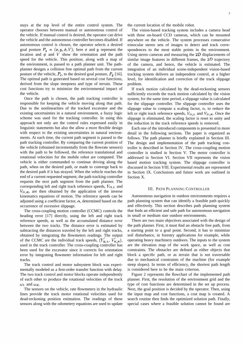
II. MOTION CONTROL SYSTEM OVERVIEW
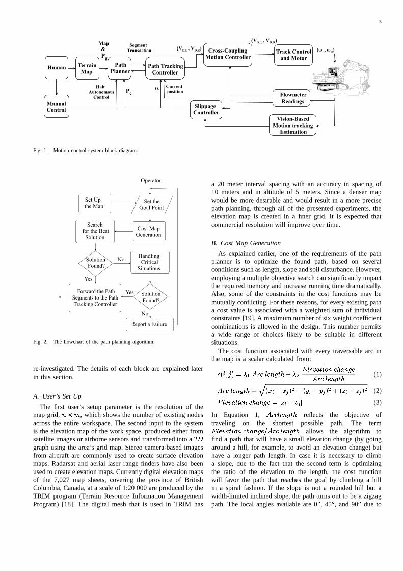
A block diagram of the semi-autonomous vehicle motioncontrol system is shown in Figure 1. The human operator
2
stays at the top level of the entire control system. Theoperator chooses between manual or autonomous control ofthe vehicle. If manual control is desired, the operator can drivethe vehicle and the autonomous controller becomes disabled. Ifautonomous control is chosen, the operator selects a desiredgoal posture
������� �� �� ��� ��; here
�and
represent the
location and�
and
show the orientation and the pathspeed for the vehicle. This position, along with a map ofthe environment, is passed to a path planner unit. The path-planner designs a collision free optimal path from the currentposture of the vehicle,
��, to the desired goal posture,
���[16].
The optimal path is generated based on several cost functions,derived from the slope steepness and type of terrain. Thesecost functions try to minimize the environmental impact ofthe vehicle.
Once the path is chosen, the path tracking controller isresponsible for keeping the vehicle moving along that path.Due to the nonlinearities of the tracked excavator and theexisting uncertainties in a natural environment, a fuzzy logicscheme was used for the tracking controller. In using thisapproach not only are the control rules expressed easily inlinguistic statements but also the allow a more flexible designwith respect to the existing uncertainties in natural environ-ments. At each time, the current path segment is passed to thepath tracking controller. By comparing the current position ofthe vehicle (obtained incrementally from the flowrate sensors)with the path to be followed, the reference translational androtational velocities for the mobile robot are computed. Thevehicle is either commanded to continue driving along thepath, when on the desired path, or made to converge back tothe desired path if it has strayed. When the vehicle reaches theend of a current requested segment, the path tracking controllerrequests the next path segment from the path planner. Thecorresponding left and right track reference speeds,
���� �and ���� �
, are then obtained by the application of the inversekinematics equations of motion. The reference speeds can beadjusted using a coefficient factor, � , determined based on theoccurrence of excessive slippage.
The cross-coupling motion controller (CCMC) controls theheading error [17] directly, using the left and right trackreference speeds, as well as the accumulated distance errorbetween the two tracks. The distance error is estimated bysubtracting the distances traveled by the left and right tracks,obtained by integrating the flowmeters readings. The outputof the CCMC are the individual track speeds,
� ����� �, ����� � �
,used in the track controller. The cross-coupling controller hasbeen used for the excavator since it corrects for orientationerror by integrating flowmeter information for left and righttracks.
The track control and motor subsystem block was experi-mentally modeled as a first-order transfer function with delay.The two track control and motor blocks operate independentlyof each other to produce the rotational velocities of the track� � and � � .
The sensors on the vehicle, rate flowmeters in the hydrauliclines provide the track motor rotational velocities used fordead-reckoning position estimation. The readings of thesesensors along with the odometery equations are used to update
the current location of the mobile robot.The vision-based tracking system includes a camera head
with three on-board CCD cameras, which can be mountedanywhere on the vehicle. The system processes consecutivetrinocular stereo sets of images to detect and track corre-spondences to the most stable points in the environment.Using stereo cameras and measuring the � � displacements ofsimilar image features in different frames, the � � trajectoryof the camera, and hence, the vehicle is estimated. Theintegration of an individual scene-independent vision-basedtracking system delivers an independent control, at a higherlevel, for identification and correction of the track slippageproblem.
If track motion calculated by the dead-reckoning sensorssufficiently exceeds the track motion calculated by the visionsystem, for the same time period, a slippage value is calculatedfor the slippage controller. The slippage controller uses theslippage value to compute a scaling factor, � , to reduce theleft or right track reference speeds,
���� �and
���� �. Once the
slippage is eliminated, the scaling factor is reset to unity andthe reduction in the track reference speeds is removed.
Each one of the introduced components is presented in moredetail in the following sections. The paper is organized asfollows. The path planner is briefly explained in Section III.The design and implementation of the path tracking con-troller is described in Section IV. The cross-coupling motioncontroller is studied in Section V. The motor controller isaddressed in Section VI. Section VII represents the visionbased motion tracking system. The slippage controller isdiscussed in Section VIII. Experimental results are representedin Section IX. Conclusions and future work are outlined inSection X.
III. PATH PLANNING CONTROLLER
Autonomous navigation in outdoor environments requires apath planning system that can identify a feasible path quicklyand effectively. This section describes path planning systemthat finds an efficient and safe path for autonomous navigationin small or medium size outdoor environments.
There are two main objectives associated with the design ofthe path planner. First, it must find an obstacle free path, froma starting point to a goal point. Second, it has to minimizesoil disturbance, in forestry applications for example, whileoperating heavy machinery outdoors. The inputs to the systemare the elevation map of the work space, as well as costconstraints. The obstacles are defined as either objects thatblock a specific path, or as terrain that is not traversabledue to mechanical constraints of the machine (for examplesteep slopes). In terms of efficiency, the shortest path lengthis considered here to be the main criterion.
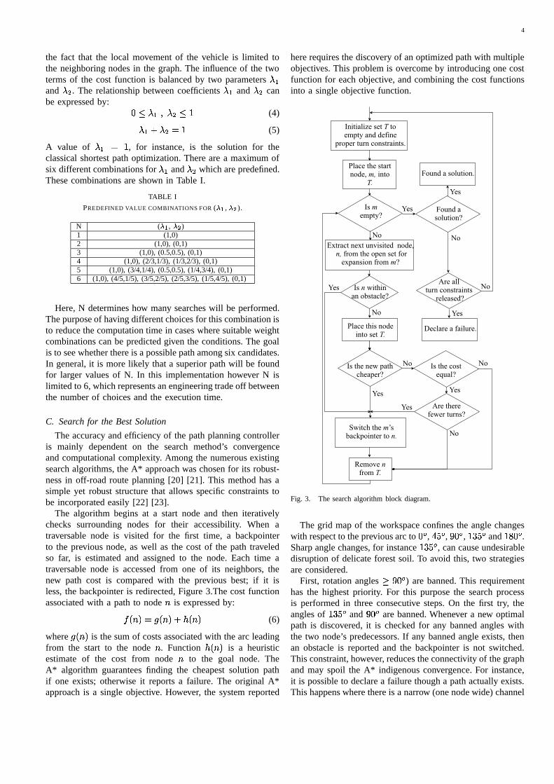
Figure 2 represents the flowchart of the implemented pathplanner. First, the resolution of the environment grid and thetype of cost functions are determined in the set up process.Next, the goal position is decided by the operator. Then, usingthe input map and cost functions, a cost map is created. Asearch routine then finds the optimized solution path. Finally,special cases where a feasible solution cannot be found are
3
TerrainMap
PathPlanner
Path TrackingController
Cross-CouplingMotion Controller
Track Controland Motor
SlippageController
FlowmeterReadings
Vision-BasedMotion tracking
Estimation
(V , V )D,L D,R
(V , V )’ ’
R,L R,R
( , )w wL R
aPc
Map&
Pg
Human
ManualControl
HaltAutonomous
Control
SegmentTransaction
Currentposition
Fig. 1. Motion control system block diagram.
Cost MapGeneration
Set Upthe Map
Set theGoal Point
Searchfor the BestSolution
SolutionFound?
HandlingCritical
Situations
SolutionFound?
Forward the PathSegments to the PathTracking Controller
Report a Failure
Operator
Yes
No
Yes
No
Fig. 2. The flowchart of the path planning algorithm.
re-investigated. The details of each block are explained laterin this section.
A. User’s Set Up
The first user’s setup parameter is the resolution of themap grid, ����� , which shows the number of existing nodesacross the entire workspace. The second input to the systemis the elevation map of the work space, produced either fromsatellite images or airborne sensors and transformed into a � �graph using the area’s grid map. Stereo camera-based imagesfrom aircraft are commonly used to create surface elevationmaps. Radarsat and aerial laser range finders have also beenused to create elevation maps. Currently digital elevation mapsof the 7,027 map sheets, covering the province of BritishColumbia, Canada, at a scale of 1:20 000 are produced by theTRIM program (Terrain Resource Information ManagementProgram) [18]. The digital mesh that is used in TRIM has
a 20 meter interval spacing with an accuracy in spacing of10 meters and in altitude of 5 meters. Since a denser mapwould be more desirable and would result in a more precisepath planning, through all of the presented experiments, theelevation map is created in a finer grid. It is expected thatcommercial resolution will improve over time.
B. Cost Map Generation
As explained earlier, one of the requirements of the pathplanner is to optimize the found path, based on severalconditions such as length, slope and soil disturbance. However,employing a multiple objective search can significantly impactthe required memory and increase running time dramatically.Also, some of the constraints in the cost functions may bemutually conflicting. For these reasons, for every existing patha cost value is associated with a weighted sum of individualconstraints [19]. A maximum number of six weight coefficientcombinations is allowed in the design. This number permitsa wide range of choices likely to be suitable in differentsituations.
The cost function associated with every traversable arc inthe map is a scalar calculated from:
� � � � � � ��� � �� ��� � ��� � ��� ��� � � � � � � � � � � � � � ��� � �� ��� � ��� � � (1)
�� ��� � ��� � � ��� � ���� � ! � � � � �� ! � � � � " �� #" ! � � (2)
� � � � � � � � � � � � ��� � �%$ " �� �" ! $ (3)
In Equation 1, �� � � � ��� � � reflects the objective of
traveling on the shortest possible path. The term� � � � � � � � � � � � ��� � & �� ��� � ��� � � allows the algorithm tofind a path that will have a small elevation change (by goingaround a hill, for example, to avoid an elevation change) buthave a longer path length. In case it is necessary to climba slope, due to the fact that the second term is optimizingthe ratio of the elevation to the length, the cost functionwill favor the path that reaches the goal by climbing a hillin a spiral fashion. If the slope is not a rounded hill but awidth-limited inclined slope, the path turns out to be a zigzagpath. The local angles available are 0 ' , 45 ' , and 90 ' due to
4
the fact that the local movement of the vehicle is limited tothe neighboring nodes in the graph. The influence of the twoterms of the cost function is balanced by two parameters
� and
���. The relationship between coefficients
� and
���can
be expressed by: ��� �� � ��� ���(4)�� � ��� � � (5)
A value of�� � �
, for instance, is the solution for theclassical shortest path optimization. There are a maximum ofsix different combinations for
� and���
which are predefined.These combinations are shown in Table I.
TABLE I
PREDEFINED VALUE COMBINATIONS FOR ( � � , � � ).
N ( � � , � � )1 (1,0)2 (1,0), (0,1)3 (1,0), (0.5,0.5), (0,1)4 (1,0), (2/3,1/3), (1/3,2/3), (0,1)5 (1,0), (3/4,1/4), (0.5,0.5), (1/4,3/4), (0,1)6 (1,0), (4/5,1/5), (3/5,2/5), (2/5,3/5), (1/5,4/5), (0,1)
Here, N determines how many searches will be performed.The purpose of having different choices for this combination isto reduce the computation time in cases where suitable weightcombinations can be predicted given the conditions. The goalis to see whether there is a possible path among six candidates.In general, it is more likely that a superior path will be foundfor larger values of N. In this implementation however N islimited to 6, which represents an engineering trade off betweenthe number of choices and the execution time.
C. Search for the Best Solution
The accuracy and efficiency of the path planning controlleris mainly dependent on the search method’s convergenceand computational complexity. Among the numerous existingsearch algorithms, the A* approach was chosen for its robust-ness in off-road route planning [20] [21]. This method has asimple yet robust structure that allows specific constraints tobe incorporated easily [22] [23].
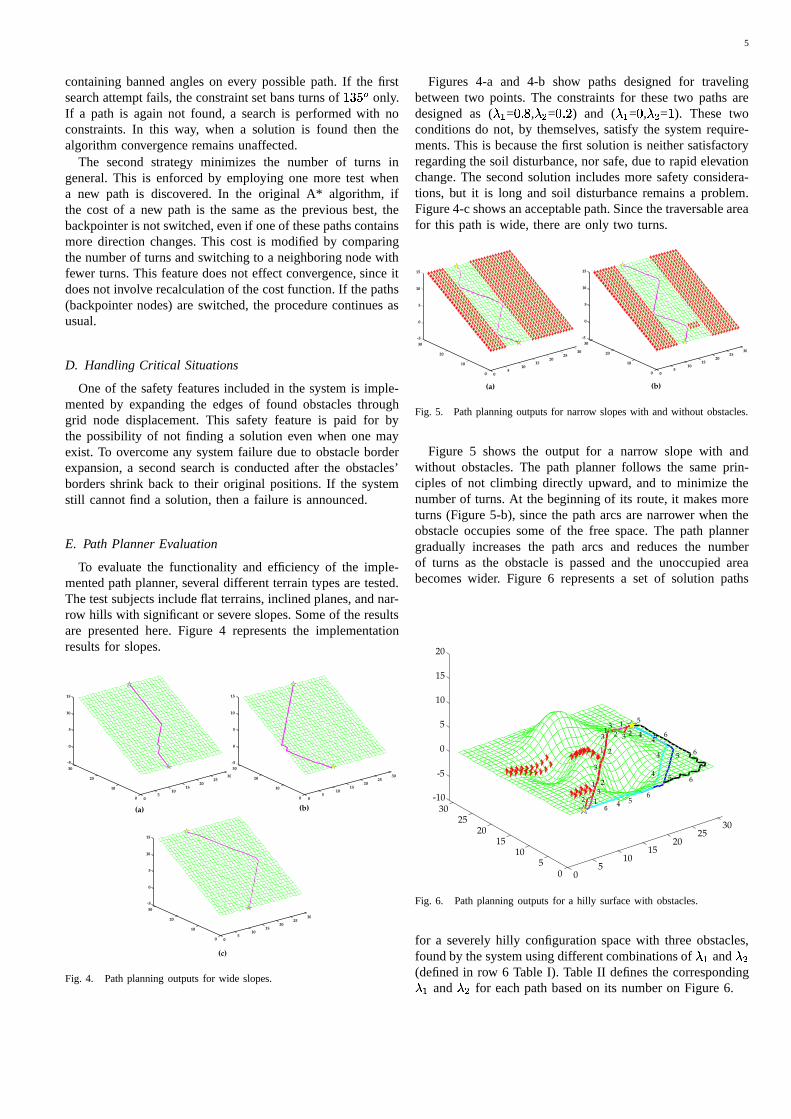
The algorithm begins at a start node and then iterativelychecks surrounding nodes for their accessibility. When atraversable node is visited for the first time, a backpointerto the previous node, as well as the cost of the path traveledso far, is estimated and assigned to the node. Each time atraversable node is accessed from one of its neighbors, thenew path cost is compared with the previous best; if it isless, the backpointer is redirected, Figure 3.The cost functionassociated with a path to node � is expressed by:
� � � � � � � � � � � � � (6)
where � � � � is the sum of costs associated with the arc leadingfrom the start to the node � . Function � � � � is a heuristicestimate of the cost from node � to the goal node. TheA* algorithm guarantees finding the cheapest solution pathif one exists; otherwise it reports a failure. The original A*approach is a single objective. However, the system reported
here requires the discovery of an optimized path with multipleobjectives. This problem is overcome by introducing one costfunction for each objective, and combining the cost functionsinto a single objective function.
Place the startnode, intom,
T.
Isempty?
m Found asolution?
Extract next unvisited node,from the open set for
expansion from ?n,
m
Is withinan obstacle?
n
Initialize set toempty and define
proper turn constraints.
T
Place this nodeinto set T.
Switch the ’sbackpointer to
m
n.
Is the new pathcheaper?
Is the costequal?
Removefrom
n
T.
Are therefewer turns?
Are allturn constraints
released?
Declare a failure.
Found a solution.
Yes
Yes
Yes
No
No
No
No
No
Yes
No
Yes
Yes
No
Yes
Fig. 3. The search algorithm block diagram.
The grid map of the workspace confines the angle changeswith respect to the previous arc to
� ' , � ' , � � ' , � � � ' and� � ' .
Sharp angle changes, for instance� � � ' , can cause undesirable
disruption of delicate forest soil. To avoid this, two strategiesare considered.
First, rotation angles ��� � ' ) are banned. This requirementhas the highest priority. For this purpose the search processis performed in three consecutive steps. On the first try, theangles of
� � � ' and � � ' are banned. Whenever a new optimalpath is discovered, it is checked for any banned angles withthe two node’s predecessors. If any banned angle exists, thenan obstacle is reported and the backpointer is not switched.This constraint, however, reduces the connectivity of the graphand may spoil the A* indigenous convergence. For instance,it is possible to declare a failure though a path actually exists.This happens where there is a narrow (one node wide) channel
5
containing banned angles on every possible path. If the firstsearch attempt fails, the constraint set bans turns of
� � � ' only.If a path is again not found, a search is performed with noconstraints. In this way, when a solution is found then thealgorithm convergence remains unaffected.
The second strategy minimizes the number of turns ingeneral. This is enforced by employing one more test whena new path is discovered. In the original A* algorithm, ifthe cost of a new path is the same as the previous best, thebackpointer is not switched, even if one of these paths containsmore direction changes. This cost is modified by comparingthe number of turns and switching to a neighboring node withfewer turns. This feature does not effect convergence, since itdoes not involve recalculation of the cost function. If the paths(backpointer nodes) are switched, the procedure continues asusual.
D. Handling Critical Situations
One of the safety features included in the system is imple-mented by expanding the edges of found obstacles throughgrid node displacement. This safety feature is paid for bythe possibility of not finding a solution even when one mayexist. To overcome any system failure due to obstacle borderexpansion, a second search is conducted after the obstacles’borders shrink back to their original positions. If the systemstill cannot find a solution, then a failure is announced.
E. Path Planner Evaluation
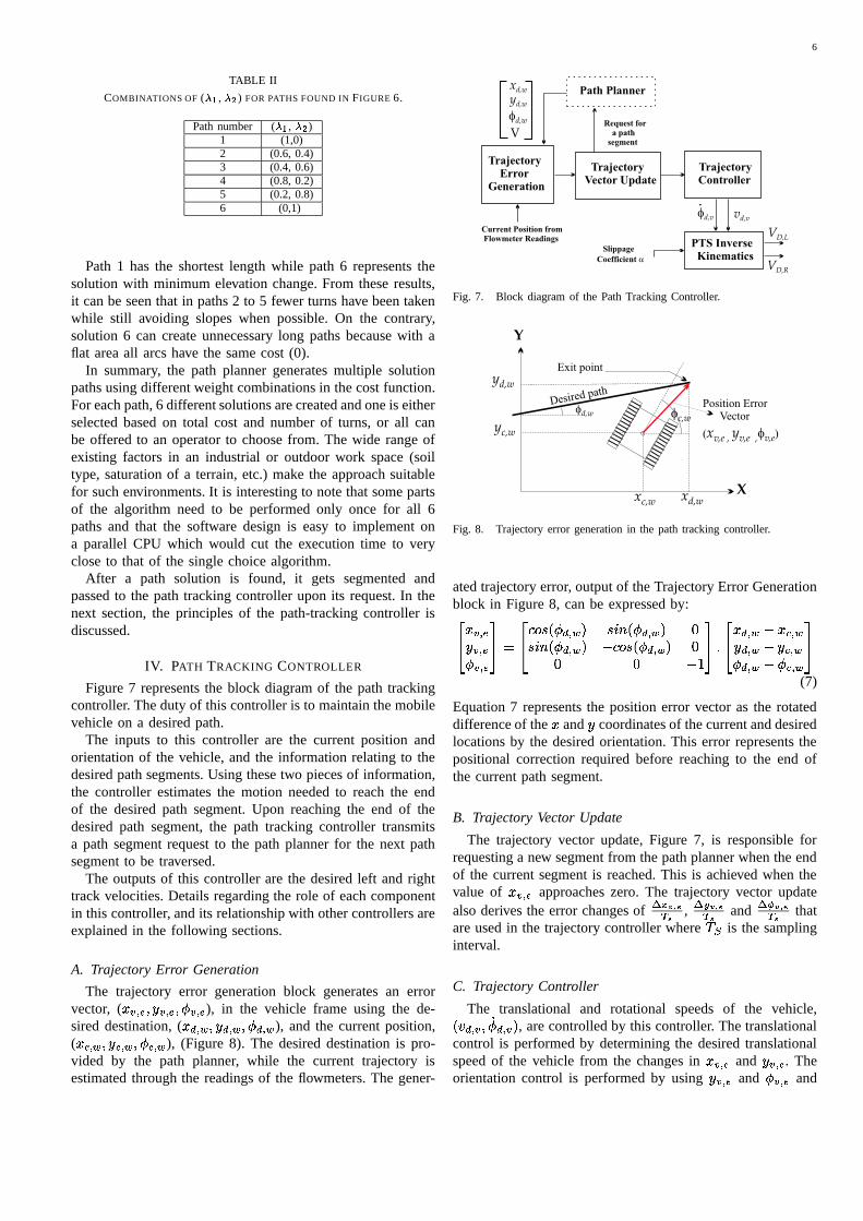
To evaluate the functionality and efficiency of the imple-mented path planner, several different terrain types are tested.The test subjects include flat terrains, inclined planes, and nar-row hills with significant or severe slopes. Some of the resultsare presented here. Figure 4 represents the implementationresults for slopes.
05
1015
2025
30
0
10
20
30-5
0
5
10
15
05
1015
2025
30
0
10
20
30-5
0
5
10
15
05
1015
2025
30
0
10
20
30-5
0
5
10
15
(c)
(a) (b)
Fig. 4. Path planning outputs for wide slopes.
Figures 4-a and 4-b show paths designed for travelingbetween two points. The constraints for these two paths aredesigned as (
��=� �
,���
=� � � ) and (
��=�,���
=�). These two
conditions do not, by themselves, satisfy the system require-ments. This is because the first solution is neither satisfactoryregarding the soil disturbance, nor safe, due to rapid elevationchange. The second solution includes more safety considera-tions, but it is long and soil disturbance remains a problem.Figure 4-c shows an acceptable path. Since the traversable areafor this path is wide, there are only two turns.
05
1015
2025
30
0
10
20
30-5
0
5
10
15
05
1015
2025
30
0
10
20
30 -5
0
5
10
15
(a) (b)
Fig. 5. Path planning outputs for narrow slopes with and without obstacles.
Figure 5 shows the output for a narrow slope with andwithout obstacles. The path planner follows the same prin-ciples of not climbing directly upward, and to minimize thenumber of turns. At the beginning of its route, it makes moreturns (Figure 5-b), since the path arcs are narrower when theobstacle occupies some of the free space. The path plannergradually increases the path arcs and reduces the numberof turns as the obstacle is passed and the unoccupied areabecomes wider. Figure 6 represents a set of solution paths
3
05
1015
2025
30
05
1015
2025
30-10
-5
0
5
10
15
20
1
2 4
56
3
1
1
11
2
2
2
2
33
4
4
4
4
5
5
5
5
6
6
6
63
3
Fig. 6. Path planning outputs for a hilly surface with obstacles.
for a severely hilly configuration space with three obstacles,found by the system using different combinations of
� and���
(defined in row 6 Table I). Table II defines the corresponding��and
���for each path based on its number on Figure 6.
6
TABLE II
COMBINATIONS OF ( � � , � � ) FOR PATHS FOUND IN FIGURE 6.
Path number ( � � , � � )1 (1,0)2 (0.6, 0.4)3 (0.4, 0.6)4 (0.8, 0.2)5 (0.2, 0.8)6 (0,1)
Path 1 has the shortest length while path 6 represents thesolution with minimum elevation change. From these results,it can be seen that in paths 2 to 5 fewer turns have been takenwhile still avoiding slopes when possible. On the contrary,solution 6 can create unnecessary long paths because with aflat area all arcs have the same cost (0).
In summary, the path planner generates multiple solutionpaths using different weight combinations in the cost function.For each path, 6 different solutions are created and one is eitherselected based on total cost and number of turns, or all canbe offered to an operator to choose from. The wide range ofexisting factors in an industrial or outdoor work space (soiltype, saturation of a terrain, etc.) make the approach suitablefor such environments. It is interesting to note that some partsof the algorithm need to be performed only once for all 6paths and that the software design is easy to implement ona parallel CPU which would cut the execution time to veryclose to that of the single choice algorithm.
After a path solution is found, it gets segmented andpassed to the path tracking controller upon its request. In thenext section, the principles of the path-tracking controller isdiscussed.
IV. PATH TRACKING CONTROLLER
Figure 7 represents the block diagram of the path trackingcontroller. The duty of this controller is to maintain the mobilevehicle on a desired path.
The inputs to this controller are the current position andorientation of the vehicle, and the information relating to thedesired path segments. Using these two pieces of information,the controller estimates the motion needed to reach the endof the desired path segment. Upon reaching the end of thedesired path segment, the path tracking controller transmitsa path segment request to the path planner for the next pathsegment to be traversed.
The outputs of this controller are the desired left and righttrack velocities. Details regarding the role of each componentin this controller, and its relationship with other controllers areexplained in the following sections.
A. Trajectory Error Generation
The trajectory error generation block generates an errorvector, (
��� � � � � � � � ��� � � ), in the vehicle frame using the de-sired destination, (
��� � � � � � � � ��� � �), and the current position,
(��� � ��� � � � � ��� � �
), (Figure 8). The desired destination is pro-vided by the path planner, while the current trajectory isestimated through the readings of the flowmeters. The gener-
TrajectoryError
Generation
TrajectoryVector Update
Path Planner
TrajectoryController
Request fora path
segment
PTS InverseKinematics
Current Position fromFlowmeter Readings
Slippage
Coefficient a
Fig. 7. Block diagram of the Path Tracking Controller.
yd,w
yc,w
xc,w xd,wX
Y
Desired path
Exit point
fd,w fc,w
Position ErrorVector
(x yv,e , v,e ,fv,e)
Fig. 8. Trajectory error generation in the path tracking controller.
ated trajectory error, output of the Trajectory Error Generationblock in Figure 8, can be expressed by:�� ��� � � � � ���� � �
���� � � � ��� � ���� � � � ��� � �� � � � � ��� � �� � � � ��� � ��� �
� � �� � �� ��� � � ��� � � � � � � � �
��� � � ��� � ��
(7)
Equation 7 represents the position error vector as the rotateddifference of the
�and
coordinates of the current and desired
locations by the desired orientation. This error represents thepositional correction required before reaching to the end ofthe current path segment.
B. Trajectory Vector Update
The trajectory vector update, Figure 7, is responsible forrequesting a new segment from the path planner when the endof the current segment is reached. This is achieved when thevalue of
��� � � approaches zero. The trajectory vector updatealso derives the error changes of �� � � �� � , ��� � � �� � and ��� � � �� � thatare used in the trajectory controller where ��� is the samplinginterval.
C. Trajectory Controller
The translational and rotational speeds of the vehicle,� � � � � ������ � � � , are controlled by this controller. The translationalcontrol is performed by determining the desired translationalspeed of the vehicle from the changes in
��� � � and � � � . The
orientation control is performed by using � � � and
��� � � and
7
their derivatives to derive the desired rotational velocity of thevehicle. The goal is to converge the inputs to zero:
� � � � � ��� � � ���� � �(8)
��� � � � � � � ��� � ���� � �(9)
1) Translational Speed Controller: Regardless of the posi-tion and orientation, this controller is responsible for maintain-ing a desired acceleration during the starting time and speedchange when converging to a desired translational speed. Itis also responsible for stopping at an exact, user specifiedposition with a desired deceleration. Here, the sum of changesin�
and
of the vehicle are measured to estimate the actualspeed of the vehicle. The control rules for converging to, ormaintaining, a desired action can be expressed as:� � � � �
��� � � � � if ��� � �if �� (10)
where � �� � � ��� � ����� �� � � � � �����
�(11)
These equations state that the desired velocity of the excavatoris increased (decreased) if the excavator Euclidean velocity
required to eliminate the error in one time step is less than(greater than) the velocity � specified by the path planner(where
is bounded by the maximum permitted excavator
speed).At each turning point the translational speed has to be
decreased to prevent the vehicle from overshooting whenconverging to a new path. In order to ensure a stop at an exactstop position with a specific deceleration
� � ' � , the followingrules [24] are adopted:
� � � � � ��� � � � � sign� ��� � � � � � � � � � ' � � $ ��� � � $ (12)
� � � � ���� ����� ��� �
if � � � � � ��� � � ��� � � ' � � if �� � � � � � ��� � � � � � ' � � if ��� � � � � � ��� � � � (13)
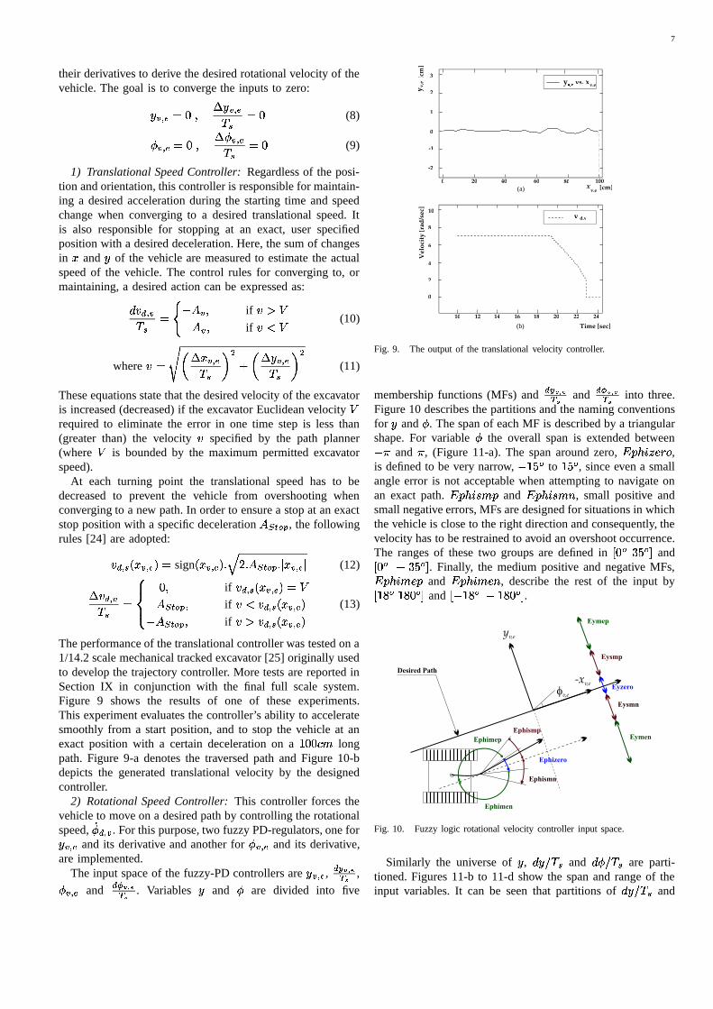
The performance of the translational controller was tested on a1/14.2 scale mechanical tracked excavator [25] originally usedto develop the trajectory controller. More tests are reported inSection IX in conjunction with the final full scale system.Figure 9 shows the results of one of these experiments.This experiment evaluates the controller’s ability to acceleratesmoothly from a start position, and to stop the vehicle at anexact position with a certain deceleration on a
� � � � � longpath. Figure 9-a denotes the traversed path and Figure 10-bdepicts the generated translational velocity by the designedcontroller.
2) Rotational Speed Controller: This controller forces thevehicle to move on a desired path by controlling the rotationalspeed,
���� � �. For this purpose, two fuzzy PD-regulators, one for � � � and its derivative and another for
��� � � and its derivative,are implemented.
The input space of the fuzzy-PD controllers are � � � , � � � � �� � ,��� � � and
� � � � �� � . Variables
and�
are divided into five
-2
-1
0
1
2
3
0 20 40 60 100
y vs. x
x v,e
v,ey y v,e
d,v
Time [sec]
Vel
ocit
y [r
ad/s
ec]
y v,e
80[cm]
[cm
]
(a)
0
2
4
6
8
10
10 12 14 16 18 20 22 24
v
(b)
Fig. 9. The output of the translational velocity controller.
membership functions (MFs) and� � � � �� � and
� � � � �� � into three.Figure 10 describes the partitions and the naming conventionsfor
and�
. The span of each MF is described by a triangularshape. For variable
�the overall span is extended between ��
and�
, (Figure 11-a). The span around zero, ��� � � " � � � ,is defined to be very narrow,
� � ' to� � ' , since even a small
angle error is not acceptable when attempting to navigate onan exact path. ��� � � � � and ��� � � ��� , small positive andsmall negative errors, MFs are designed for situations in whichthe vehicle is close to the right direction and consequently, thevelocity has to be restrained to avoid an overshoot occurrence.The ranges of these two groups are defined in � � ' � � ' � and� � ' � � ' � . Finally, the medium positive and negative MFs,��� � � � � � and ��� � � � � � , describe the rest of the input by� � ' � � ' � and � � ' � � ' � .
Desired Path
Ephimen
Ephizero
Ephismn
Ephimep
Ephismp
fv,e
yv,e
-xv,e
Eymen
Eyzero
Eysmn
Eymep
Eysmp
Fig. 10. Fuzzy logic rotational velocity controller input space.
Similarly the universe of
,� & ��� and
� � & ��� are parti-tioned. Figures 11-b to 11-d show the span and range of theinput variables. It can be seen that partitions of
� & ��� and
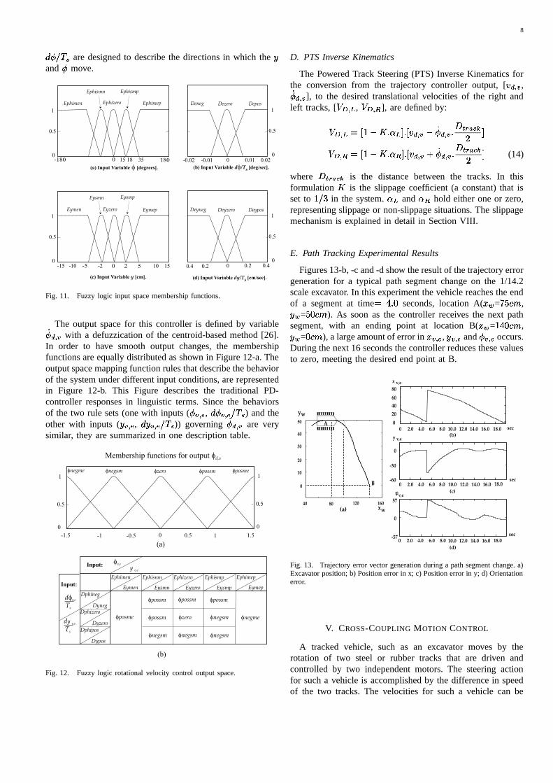
8� � & ��� are designed to describe the directions in which the
and�
move.
1
0
0.5
0 0.01-0.01 0
1
0
0.5
Ephimen
Ephismn
Ephizero
Ephismp
Ephimep Deneg Dezero Depos
1
0
0.5
-5 0 0.2 0.40.4 0.2 0
1
0
0.5
Eymen
Eysmn
Eyzero
Eysmp
Eymep Deyneg Deyzero Deypos
-180 180 0.02-0.02
52-2 10 15-15 -10
(a) Input Variable [degrees].f (b) Input Variable df/Ts [deg/sec].
(c) Input Variable [cm].y (d) Input Variable dy/Ts
18 3515
[cm/sec].
Fig. 11. Fuzzy logic input space membership functions.
The output space for this controller is defined by variable���� � �with a defuzzication of the centroid-based method [26].
In order to have smooth output changes, the membershipfunctions are equally distributed as shown in Figure 12-a. Theoutput space mapping function rules that describe the behaviorof the system under different input conditions, are representedin Figure 12-b. This Figure describes the traditional PD-controller responses in linguistic terms. Since the behaviorsof the two rule sets (one with inputs (
��� � � , � ��� � � & ��� ) and theother with inputs (
� � � , � � � � & ��� )) governing���� � �
are verysimilar, they are summarized in one description table.
Dphipos
Dphineg
DphizeroDyneg
Dyzero
Dypos
Ephimen
Eymen
Ephismn
Eysmn
Ephizero
Eyzero
Ephismp
Eysmp
Ephimep
Eymep
y v,e
Input:fv,e
Input:
dfv,e
dy v,e
Ts
Ts
fposme
fpossm fpossm
fnegsm
fzero
fpossm
fnegsm
fpossm fnegme
fnegsm
fnegsm
fzero fpossmfnegsm fposmefnegme1
0
0.5
1
0
0.5
-1.5 -1 -0.5 0 0.5 1 1.5
Membership functions for output fd,v
.
(a)
(b)
.
....
..
.
.
..
..
..
.
Fig. 12. Fuzzy logic rotational velocity control output space.
D. PTS Inverse Kinematics
The Powered Track Steering (PTS) Inverse Kinematics forthe conversion from the trajectory controller output, [ � � � � ,���� � �
], to the desired translational velocities of the right andleft tracks, [
���� �, ���� �
], are defined by:
���� � � � � �� � � � � � � � � � � ���� � � � � � � � � �� � ���� � � � � �� � � � � � � � � � � � ���� � � � � � � � � �
� � (14)
where � � � � � � is the distance between the tracks. In thisformulation
�is the slippage coefficient (a constant) that is
set to� & � in the system. � � and � � hold either one or zero,
representing slippage or non-slippage situations. The slippagemechanism is explained in detail in Section VIII.
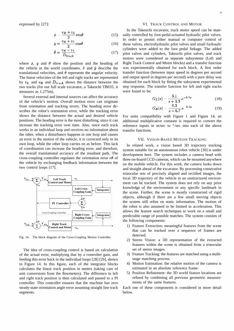
E. Path Tracking Experimental Results
Figures 13-b, -c and -d show the result of the trajectory errorgeneration for a typical path segment change on the 1/14.2scale excavator. In this experiment the vehicle reaches the endof a segment at time
� � � seconds, location A(���
= � � � � , �= � � � � ). As soon as the controller receives the next path
segment, with an ending point at location B(���
=� � � � , �
=� � � ), a large amount of error in
��� � � , � � � and��� � � occurs.
During the next 16 seconds the controller reduces these valuesto zero, meeting the desired end point at B.
y v,e
sec
sec
sec
80
0
204060
0 2.0 4.0 6.0 8.0 10.0 12.0 14.0 16.0 18.0
0
-30
-60
57
0
-57
0 2.0 4.0 6.0 8.0 10.0 12.0 14.0 16.0 18.0
0 2.0 4.0 6.0 8.0 10.0 12.0 14.0 16.0 18.0
φ v,e
x v,e
xw
yw
40 80 120 160
0
10
20
30
50
40
(a)
(c)
(d)
(b)
B
A
Fig. 13. Trajectory error vector generation during a path segment change. a)Excavator position; b) Position error in x; c) Position error in y; d) Orientationerror.
V. CROSS-COUPLING MOTION CONTROL
A tracked vehicle, such as an excavator moves by therotation of two steel or rubber tracks that are driven andcontrolled by two independent motors. The steering actionfor such a vehicle is accomplished by the difference in speedof the two tracks. The velocities for such a vehicle can be
9
expressed by [27]:
�� � � � � � ��
� ��� (15)
� � � � � � ��
� � � (16)�� � � �� � �� � � � � � (17)
where�
,
and � show the position and the heading ofthe vehicle in the world coordinates, �� and � describe thetranslational velocities, and
�� represents the angular velocity.The linear velocities of the left and right tracks are representedby � � and � � and � � � � � � shows the distance between thetwo tracks (for our full scale excavator, a Takeuchi TB035, itmeasures as 1.275m).
Several external and internal sources can affect the accuracyof the vehicle’s motion. Overall motion error can originatefrom orientation and tracking errors. The heading error de-scribes the robot’s orientation error, while the tracking errorshows the distance between the actual and desired vehiclepositions. The heading error is the most disturbing, since it canincrease the tracking error over time. Also, since each trackworks in an individual loop and receives no information aboutthe other, when a disturbance happens in one loop and causesan error in the motion of the vehicle, it is corrected only in itsown loop, while the other loop carries on as before. This lackof coordination can increase the heading error, and therefore,the overall translational accuracy of the resultant path. Thecross-coupling controller regulates the orientation error � � ofthe vehicle by exchanging feedback information between thetwo control loops [17].
SS
S
SSVD,L
VD,R
V’
R,L
V’
R,R
wL
PI Controller
Left TrackControl and Motor
Left Cross-Coupling Gain
Right Cross-Coupling Gain
Integrator
Integrator
+
-
-
+
++
Cross-Coupling Controller
Right TrackControl and Motor wR
Fig. 14. The block diagram of the Cross-Coupling Motion Controller.
The idea of cross-coupling control is based on calculationof the actual error, multiplying that by a controller gain, andfeeding this error back to the individual loops [28] [29], shownin Figure 14. In this figure, each of the integrator blockscalculates the linear track position in meters (taking care ofunit conversions from the flowmeters). The difference in leftand right track position is then calculated and passed to a PIcontroller. This controller ensures that the machine has zerosteady-state orientation angle error assuming straight line tracksegments.
VI. TRACK CONTROL AND MOTOR
In the Takeuchi excavator, track motor speed can be man-ually controlled by foot-pedal-actuated hydraulic pilot valves.In order to permit either manual or computer control ofthese valves, electrohydraulic pilot valves and small hydrauliccylinders were added to the foot pedal linkage. The addedpilot valves and cylinders, Takeuchi pilot valves, and trackmotors were considered as separate subsystems (Left andRight Track Control and Motor blocks) and a transfer functionwas experimentally obtained for each block. A first ordertransfer function (between input speed in degrees per secondand output speed in degrees per second) with a pure delay wasobtained for each block by fitting the subsystem experimentalstep response. The transfer function for left and right trackswere found to be:
� �� ��� � � � ��� � � � � ��� �� �
(18)
� � � ����� � � � � � � � � ��� �� � (19)
For units compatibility with Figure 1 and Figure 14, anadditional multiplicative constant is required to convert thereference inputs in m/sec to ' /sec into each of the abovetransfer functions.
VII. VISION-BASED MOTION TRACKING
In related work, a vision based 3D trajectory trackingsystem suitable for an autonomous robot vehicle [30] is underdevelopment here. The system includes a camera head withthree on-board CCD cameras, which can be mounted anywhereon the mobile vehicle. For this work, the camera looks downand straight ahead of the excavator. By processing consecutivetrinocular sets of precisely aligned and rectified images, thelocal 3D trajectory of the vehicle in an unstructured environ-ment can be tracked. The system does not rely on any priorknowledge of the environment or any specific landmark inthe scene. Further, the scene is mostly constructed of rigidobjects, although if there are a few small moving objectsthe system still relies on static information. The motion ofthe robot is also assumed to be limited in acceleration. Thisallows the feature search techniques to work on a small andpredictable range of possible matches. The system consists ofthe following components:
1) Feature Extraction: meaningful features from the scenethat can be tracked over a sequence of frames aredetected.
2) Stereo Vision: a 3D representation of the extractedfeatures within the scene is obtained from a trinocularset of stereo images.
3) Feature Tracking: the features are matched using a multi-stage matching process.
4) Motion Estimation: the relative motion of the camera isestimated in an absolute reference frame.
5) Position Refinement: the 3D world feature locations arerefined by combining all previous geometric measure-ments of the same features.
Each one of these components is considered in more detailbelow.
10
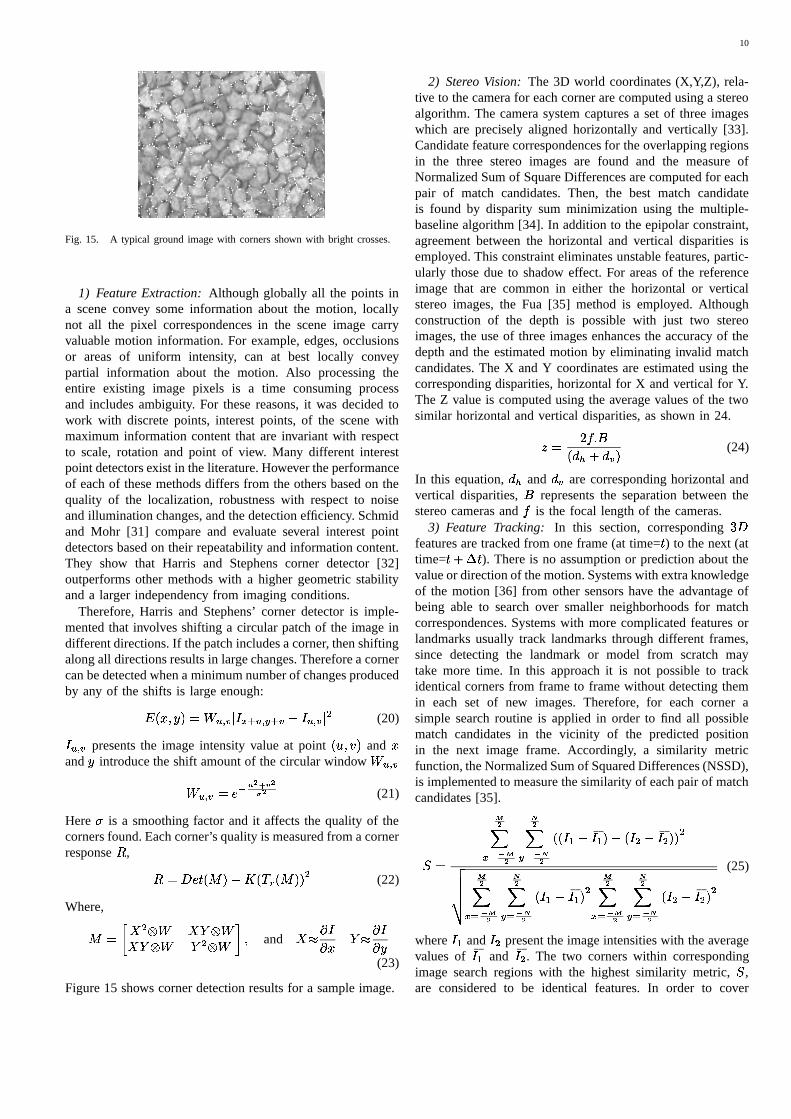
Fig. 15. A typical ground image with corners shown with bright crosses.
1) Feature Extraction: Although globally all the points ina scene convey some information about the motion, locallynot all the pixel correspondences in the scene image carryvaluable motion information. For example, edges, occlusionsor areas of uniform intensity, can at best locally conveypartial information about the motion. Also processing theentire existing image pixels is a time consuming processand includes ambiguity. For these reasons, it was decided towork with discrete points, interest points, of the scene withmaximum information content that are invariant with respectto scale, rotation and point of view. Many different interestpoint detectors exist in the literature. However the performanceof each of these methods differs from the others based on thequality of the localization, robustness with respect to noiseand illumination changes, and the detection efficiency. Schmidand Mohr [31] compare and evaluate several interest pointdetectors based on their repeatability and information content.They show that Harris and Stephens corner detector [32]outperforms other methods with a higher geometric stabilityand a larger independency from imaging conditions.
Therefore, Harris and Stephens’ corner detector is imple-mented that involves shifting a circular patch of the image indifferent directions. If the patch includes a corner, then shiftingalong all directions results in large changes. Therefore a cornercan be detected when a minimum number of changes producedby any of the shifts is large enough:
� � �� ������� � � $ � � � � � � �� �� � � � $ � (20)� � � �presents the image intensity value at point
� �� � � and�
and
introduce the shift amount of the circular window��� � �
��� � ��� � �� � � � (21)
Here is a smoothing factor and it affects the quality of thecorners found. Each corner’s quality is measured from a cornerresponse � , � � � � � � � � � � � � � � � � � (22)
Where,� ��� � � � � ��� � ���� � � � � � ��� � and ����� �� � ����� �� (23)
Figure 15 shows corner detection results for a sample image.
2) Stereo Vision: The 3D world coordinates (X,Y,Z), rela-tive to the camera for each corner are computed using a stereoalgorithm. The camera system captures a set of three imageswhich are precisely aligned horizontally and vertically [33].Candidate feature correspondences for the overlapping regionsin the three stereo images are found and the measure ofNormalized Sum of Square Differences are computed for eachpair of match candidates. Then, the best match candidateis found by disparity sum minimization using the multiple-baseline algorithm [34]. In addition to the epipolar constraint,agreement between the horizontal and vertical disparities isemployed. This constraint eliminates unstable features, partic-ularly those due to shadow effect. For areas of the referenceimage that are common in either the horizontal or verticalstereo images, the Fua [35] method is employed. Althoughconstruction of the depth is possible with just two stereoimages, the use of three images enhances the accuracy of thedepth and the estimated motion by eliminating invalid matchcandidates. The X and Y coordinates are estimated using thecorresponding disparities, horizontal for X and vertical for Y.The Z value is computed using the average values of the twosimilar horizontal and vertical disparities, as shown in 24.
"�� � � �� � � � � � � (24)
In this equation,� �
and� �
are corresponding horizontal andvertical disparities,
�represents the separation between the
stereo cameras and
is the focal length of the cameras.3) Feature Tracking: In this section, corresponding � �
features are tracked from one frame (at time=� ) to the next (attime=��� � � ). There is no assumption or prediction about thevalue or direction of the motion. Systems with extra knowledgeof the motion [36] from other sensors have the advantage ofbeing able to search over smaller neighborhoods for matchcorrespondences. Systems with more complicated features orlandmarks usually track landmarks through different frames,since detecting the landmark or model from scratch maytake more time. In this approach it is not possible to trackidentical corners from frame to frame without detecting themin each set of new images. Therefore, for each corner asimple search routine is applied in order to find all possiblematch candidates in the vicinity of the predicted positionin the next image frame. Accordingly, a similarity metricfunction, the Normalized Sum of Squared Differences (NSSD),is implemented to measure the similarity of each pair of matchcandidates [35].
� ��
!#" �$
� !#" $� � � &%� � � � �� '%� � � � �
()))* � !+" �
$ � !#" $
� � %� � � � !#" �
$ � !+" $
� � �� %� � � � (25)
where�
and� �
present the image intensities with the averagevalues of
%� and
%� �. The two corners within corresponding
image search regions with the highest similarity metric,�
,are considered to be identical features. In order to cover
11
all motions, a wide search scope is required, due to twofactors. The displacement of the features between framesis affected by the feature to camera distance, the rotationand/or the translation that may have occured. This wide searchscope increases the number of match candidates, elevating thepossibility of false matches and influences the accuracy of themotion estimation. In order to prevent false correspondencematching, a large NSSD window of 27 � 27 is used.
4) Motion Estimation: Having a set of corresponding cor-ners between each two consecutive images, motion estimationbecomes the problem of optimizing a 3D transformation thatprojects the world corners, constructed from the first image,onto the second image [37]. Although the 3D construction of2D features is a non-linear function, the problem of motionestimation is still well-behaved. This is because any 3D motionincludes rotations and translations.� Rotations are functions of the cosine of the rotation
angles.� Translation toward or away from the camera introduces aperspective distortion as a function of the inverse of thedistance from the camera.� Translation parallel to the image plane is almost linear.
Therefore, the problem of 3D motion estimation is a promisingcandidate for the application of Newton’s method, which isbased on the assumption that the function is locally linear.To minimize the probability of converging to a false localminimum, the outliers are found and eliminated during theiteration process.
With this method, at each iteration a correction vector�
iscomputed that is subtracted from the current estimate, resultingin a new estimate. If
��� � �is the vector of image coordinates� �� � � for iteration
�, then� � � � � � � � � � �
(26)
Given a vector of error measurements between the world � �features and their projections, the
�is found that eliminates
(minimizes) this error.The effect of each element of the correction vector
���on error measurement � � is the multiplication of the partialderivative of the error with respect to that parameter to thesame correction vector; this is done by considering the mainassumption, local linearity of the function
��� � � Where� � ! � � � �� ��! (27)
�is the Jacobian matrix and � � presents the error between
the predicted location of the object and actual position of thematch found in image coordinates. Each row of this matrixequation states that one measured error, � � , should be equal tothe sum of all changes in that error resulting from parametercorrection [38]. Since Equation 28 is usually over-determined,and therefore, no unique solution exists, a vector
�is found
that minimizes the � -norm of the residual.
� � ��� ���� � � � (28)
Equation 28 has the same solution as the normal equation,� � � � � � � � � � � (29)
Therefore, in each iteration of Newton’s method, the normalEquation 29 for
�using ��� decomposition [39] is solved.
To minimize the probability of converging to a false localminimum, outliers are eliminated during the iteration process,based on their positional error.
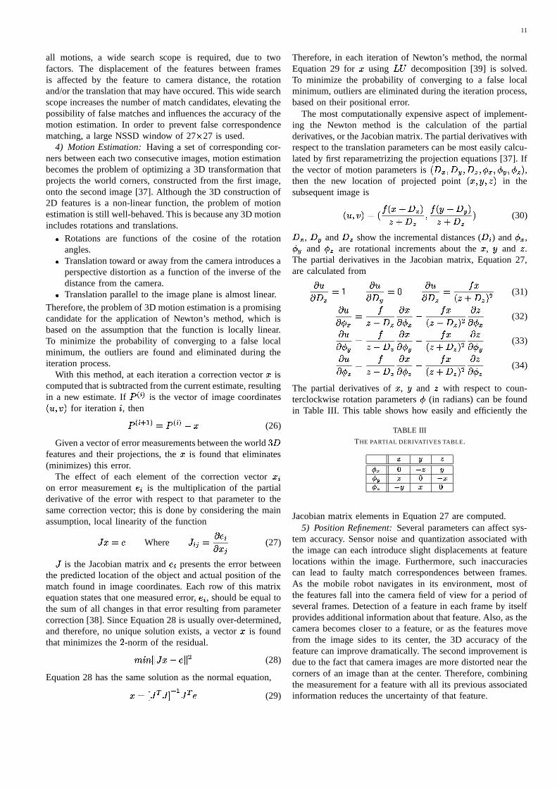
The most computationally expensive aspect of implement-ing the Newton method is the calculation of the partialderivatives, or the Jacobian matrix. The partial derivatives withrespect to the translation parameters can be most easily calcu-lated by first reparametrizing the projection equations [37]. Ifthe vector of motion parameters is
� � � � � � � � � � � � � � � ,then the new location of projected point� �� �� " �
in thesubsequent image is
� �� � ��� � � � � � �" � � � � ��� � �" � � �(30)
� , � � and � show the incremental distances ( � � ) and� ,� � and
� are rotational increments about the�
,
and".
The partial derivatives in the Jacobian matrix, Equation 27,are calculated from� �� � � � � �� � � � � � �� � �
�� " ���� � � (31)
� �� � �" � � � �� �
�� " � � � � � "� � (32)
� �� � � �" ���� � �� � �
�� " ���� � � � "� � � (33)
� �� � �" ���� � �� �
�� " � � � � � "� � (34)
The partial derivatives of�
,
and"
with respect to coun-terclockwise rotation parameters
�(in radians) can be found
in Table III. This table shows how easily and efficiently the
TABLE III
THE PARTIAL DERIVATIVES TABLE.
� � � � � � �� � � � �� � � � � �
Jacobian matrix elements in Equation 27 are computed.5) Position Refinement: Several parameters can affect sys-
tem accuracy. Sensor noise and quantization associated withthe image can each introduce slight displacements at featurelocations within the image. Furthermore, such inaccuraciescan lead to faulty match correspondences between frames.As the mobile robot navigates in its environment, most ofthe features fall into the camera field of view for a period ofseveral frames. Detection of a feature in each frame by itselfprovides additional information about that feature. Also, as thecamera becomes closer to a feature, or as the features movefrom the image sides to its center, the 3D accuracy of thefeature can improve dramatically. The second improvement isdue to the fact that camera images are more distorted near thecorners of an image than at the center. Therefore, combiningthe measurement for a feature with all its previous associatedinformation reduces the uncertainty of that feature.
12
In this system, each frame, within which a feature isdetected, gives an additional measurement for the locationof that feature. Therefore, a positional covariance is alsoassociated with each observed feature using a Kalman filtergeneration. Each filter is updated using new information forthe same feature over time. The Kalman filter provides a meansto combine these noisy measurements to form a continuousestimate of the current location of the feature. Each pointin the world space is associated with a Kalman filter, andupdated using new motion information. This process increasesthe accuracy of location information of the feature points inthe world space. A Kalman filter is implemented in a similarfashion to Shapiro’s method [40].
This formulation is recursive and the least squares estimateof the world feature position � , and its covariance
�, are given
recursively by
� �� � � �
�� � �� � � � (35)����� ���
� ��� � � � �� � � ��� � � (36)
� ��� � � �� � � (37)
In these equations�
represents the frame number. � � is theuncertainty in the estimation of
�corresponding to frame
�, � �
denotes the filter gain,� �
indicates the current measurement ofthe feature,
��represents the covariance matrix of the errors
and �
is the identity matrix. To prevent bias from distantfeatures, working in the disparity space with axes that arethe current image plane coordinates and the correspondingfeature disparity [41] is implemented. Tracking of featuresare maintained for a while, even if they move out of thecamera’s field of view. However, if a feature is not seen inthe last 6 consecutive frames it will be retired. Obviously, theerror vector for any given measurement relies on the relativeaccuracy of that measurement. The corner detector’s accuracy,which is related to the accuracy of the stereo system, originally2 pixels, is improved by fitting a sub-sample estimator [42]. Itis a simple quadratic estimator that locates the corner within apixel. The method uses neighboring intensity values and fits asecond order curve on the corner and its two neighbors. Sincethe depth construction is very sensitive to noise, this estimatorimproves the accuracy of the depth construction significantly.
6) Experimental Results: It is important to point out thatin this system the vision sub-system is used for finding therelative motion between each two consecutive frames and notthe overall trajectory of the vehicle in the global coordinatesystem. The Kalman filter helps to reduce the error in thevehicle’s trajectory over time and if the vehicle traversesaround in a bounded environment, it helps to reduce thepositional error of world features as they may be viewedseveral times from different distances. The more accurate 3Dpositional information of world features, the more accuratemotion estimation between every two frames.
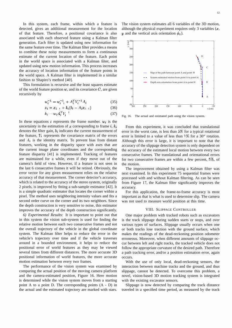
The performance of the vision system was examined bycomparing the actual position of the moving camera platformand the camera-estimated position, Figure 16. Here motionis determined while the vision system moves from a startingpoint A to a point D. The corresponding points (A - D) inthe actual and the estimated trajectory are marked with stars.
The vision system estimates all 6 variables of the 3D motion,although the physical experiment requires only 3 variables (
�,
and the vertical axis orientation� ).
-50050100150200250300-50
0
50
100
150
200
250
300
350
y [c
m]
x [cm]
A
B
C
D
Map of the path between point A and point H
System estimated motion from point A to point H
Depth axis orientation from point A to point H
Fig. 16. The actual and estimated path using the vision system.
From this experiment, it was concluded that translationalerror in the worst case, is less than � � for a typical rotationalerror is limited to a value of less than
� � for a 30 ' rotation.Although this error is large, it is important to note that theaccuracy of the slippage detection system is only dependent onthe accuracy of the estimated local motion between every twoconsecutive frames. The translational and orientational errorsfor two consecutive frames are within a few percent, � � , ofthe motion.
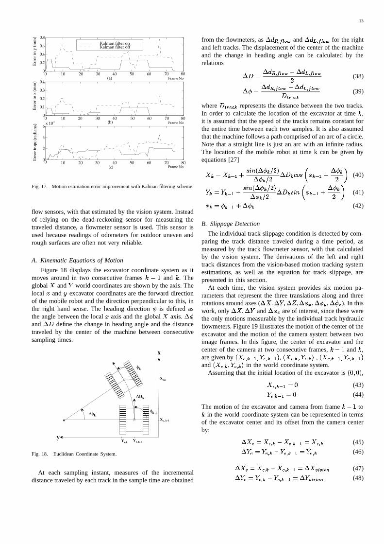
The improvement obtained by using a Kalman filter wasnext examined. In this experiment 75 sequential frames wereprocessed with and without Kalman filtering. As can be seenfrom Figure 17, the Kalman filter significantly improves theaccuracy.
For this application, the frame-to-frame accuracy is mostimportant as that is what is used to determine slip. The camerawas not used to measure world position at this time.
VIII. SLIPPAGE CONTROLLER
One major problem with tracked robots such as excavatorsis the track slippage during sudden starts or stops, and overvarious types of surfaces. Slippage usually occurs when oneor both tracks lose traction with the ground surface, whichmakes the readings of the dead-reckoning position odometererroneous. Moreover, when different amounts of slippage oc-cur between left and right tracks, the tracked vehicle does notfollow the appropriate curvature of the desired path. Thereforea path tracking error, and/or a position estimation error, againoccurs.
With the use of only local, dead-reckoning sensors, theinteraction between machine tracks and the ground, and thusslippage, cannot be detected. To overcome this problem, anovel, vision-based 3D motion tracking system is integratedwith the existing excavator sensors.
Slippage is now detected by comparing the track distancetraveled in a specified time period, as measured by the track
13
0 10 20 30 40 50 60 70 800
0.2
0.4
0.6
0.8
Frame No
Erro
r in
y (m
m)
Kalman filter onKalman filter off
0 10 20 30 40 50 60 70 800
0.1
0.2
0.3
0.4
Frame No
Erro
r in
x (m
m)
0 10 20 30 40 50 60 70 800
2
4
6x 10 4
Frame No
Erro
r in φ z
(rad
ians )
(a)
(b)
(c)
Fig. 17. Motion estimation error improvement with Kalman filtering scheme.
flow sensors, with that estimated by the vision system. Insteadof relying on the dead-reckoning sensor for measuring thetraveled distance, a flowmeter sensor is used. This sensor isused because readings of odometers for outdoor uneven andrough surfaces are often not very reliable.
A. Kinematic Equations of Motion
Figure 18 displays the excavator coordinate system as itmoves around in two consecutive frames � � and � . Theglobal � and � world coordinates are shown by the axis. Thelocal
�and
excavator coordinates are the forward direction
of the mobile robot and the direction perpendicular to this, inthe right hand sense. The heading direction
�is defined as
the angle between the local�
axis and the global � axis. � �and � � define the change in heading angle and the distancetraveled by the center of the machine between consecutivesampling times.
o
y
x
Xe,k
Xe
Ye,kYe, k-1
, k-1
fk-1
fk
DDk
Dfk
Fig. 18. Euclidean Coordinate System.
At each sampling instant, measures of the incrementaldistance traveled by each track in the sample time are obtained
from the flowmeters, as � � ��� � � ' � and � � ��� � � ' � for the rightand left tracks. The displacement of the center of the machineand the change in heading angle can be calculated by therelations � � � � � ��� � � ' � � � � ��� � � ' �� (38)� � � � � ��� � � ' �� � � ��� � � ' �� � � � � � (39)
where � � � � � � represents the distance between the two tracks.In order to calculate the location of the excavator at time � ,it is assumed that the speed of the tracks remains constant forthe entire time between each two samples. It is also assumedthat the machine follows a path comprised of an arc of a circle.Note that a straight line is just an arc with an infinite radius.The location of the mobile robot at time k can be given byequations [27]
� ��� � � � � � � � � � � & � �� � � & � ��� � � � � � � � � � � �� (40)
� ��� � � � � � � � � � � & � �� � � & � � � � � � � � � � � � � �� (41)� ��� � �
� � � � � (42)
B. Slippage Detection
The individual track slippage condition is detected by com-paring the track distance traveled during a time period, asmeasured by the track flowmeter sensor, with that calculatedby the vision system. The derivations of the left and righttrack distances from the vision-based motion tracking systemestimations, as well as the equation for track slippage, arepresented in this section.
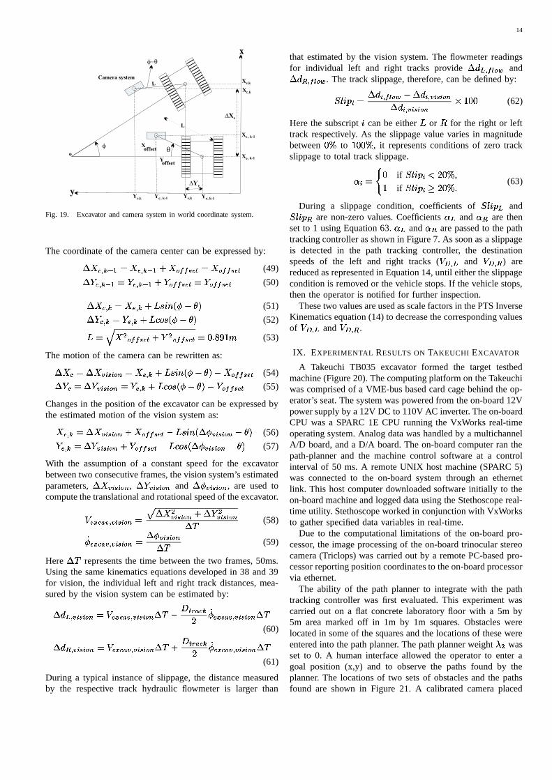
At each time, the vision system provides six motion pa-rameters that represent the three translations along and threerotations around axes ( � � � � � � ��� � � � � � � � � � � ). In thiswork, only � � � � � and � � are of interest, since these werethe only motions measurable by the individual track hydraulicflowmeters. Figure 19 illustrates the motion of the center of theexcavator and the motion of the camera system between twoimage frames. In this figure, the center of excavator and thecenter of the camera at two consecutive frames, � � and � ,are given by
� � � � � � � � � � � � � , � � � � � � � � � � � ,� � � � � � � � � � � � �
and� � � � � � � � � � � in the world coordinate system.
Assuming that the initial location of the excavator is� � � � �
,� � � � � � � (43)� � � � � � � (44)
The motion of the excavator and camera from frame � � to� in the world coordinate system can be represented in termsof the excavator center and its offset from the camera centerby: � � � � � � � � � � � � � � � � � � (45)� � � � � � � � � � � � � � � � � � (46)
� � ��� � � � � � � � � � � � � � � � � ' � (47)� � � � � � � � � � � � � � � � � � � � ' � (48)
14
Camera system
qf
L
oY
X
y
x
L
Xc,k
Xe,k
Xc
Xe
Yc,k Yc Ye,k Ye
f-q
offset
offset
, k-1 , k-1
, k-1
, k-1
DXe
DYe
Fig. 19. Excavator and camera system in world coordinate system.
The coordinate of the camera center can be expressed by:� � � � � � � � � � � � � � ' � � � � � � � ' � � � � � (49)� � � � � � � � � � � � � � ' � � � � � � � ' � � � � � (50)
� � � � ��� � � � � � � � � � �� � � (51)� � � � ��� � � � � � � � � � �� � � (52)
� � � � � ' � � � � � � � � ' � � � � � � � � � � � (53)
The motion of the camera can be rewritten as:� � ��� � � � � � � ' � � � � � � � � � � � �� � � � ' � � � � � (54)� � ��� � � � � � � ' � � � � � � � � � � � �� � � � ' � � � � � (55)
Changes in the position of the excavator can be expressed bythe estimated motion of the vision system as:� � � � � � � � � � � ' � � � ' � � � � � � � � � � ��� � � � ' � � � (56)� � � ��� � � � � � � ' � � � ' � � � � � � � � � � ��� � � � ' � � � (57)
With the assumption of a constant speed for the excavatorbetween two consecutive frames, the vision system’s estimatedparameters, � � � � � � ' � , � � � � � � ' � and � ��� � � � ' � , are used tocompute the translational and rotational speed of the excavator.
� � � � � � � � � ' � � � � � �� � � � ' � � � � �� � � � ' �� � (58)�� � � � � � � � � � ' � � � ��� � � � ' �� � (59)
Here � � represents the time between the two frames, 50ms.Using the same kinematics equations developed in 38 and 39for vision, the individual left and right track distances, mea-sured by the vision system can be estimated by:� � ��� � � � � ' � � � � � � � � � � � ' � � � � � � � � �� �� � � � � � � � � � ' � � �
(60)� � ��� � � � � ' � � � � � � � � � � � ' � � � � � � � � � �� �� � � � � � � � � � ' � � �(61)
During a typical instance of slippage, the distance measuredby the respective track hydraulic flowmeter is larger than
that estimated by the vision system. The flowmeter readingsfor individual left and right tracks provide � � ��� � � ' � and� � ��� � � ' � . The track slippage, therefore, can be defined by:� � � � ��� � � � � � � ' �� � � � � � � � � ' �� � � � � � � � ' � � � � � (62)
Here the subscript�
can be either � or � for the right or lefttrack respectively. As the slippage value varies in magnitudebetween
� � to� � � � , it represents conditions of zero track
slippage to total track slippage.
� ���� �
if� � � � � � � � ,�
if� � � � � � � � � .
(63)
During a slippage condition, coefficients of� � � � � and� � � � � are non-zero values. Coefficients � � and � � are then
set to 1 using Equation 63. � � and � � are passed to the pathtracking controller as shown in Figure 7. As soon as a slippageis detected in the path tracking controller, the destinationspeeds of the left and right tracks (
���� �and
���� �) are
reduced as represented in Equation 14, until either the slippagecondition is removed or the vehicle stops. If the vehicle stops,then the operator is notified for further inspection.
These two values are used as scale factors in the PTS InverseKinematics equation (14) to decrease the corresponding valuesof ���� �
and ���� �
.
IX. EXPERIMENTAL RESULTS ON TAKEUCHI EXCAVATOR
A Takeuchi TB035 excavator formed the target testbedmachine (Figure 20). The computing platform on the Takeuchiwas comprised of a VME-bus based card cage behind the op-erator’s seat. The system was powered from the on-board 12Vpower supply by a 12V DC to 110V AC inverter. The on-boardCPU was a SPARC 1E CPU running the VxWorks real-timeoperating system. Analog data was handled by a multichannelA/D board, and a D/A board. The on-board computer ran thepath-planner and the machine control software at a controlinterval of 50 ms. A remote UNIX host machine (SPARC 5)was connected to the on-board system through an ethernetlink. This host computer downloaded software initially to theon-board machine and logged data using the Stethoscope real-time utility. Stethoscope worked in conjunction with VxWorksto gather specified data variables in real-time.
Due to the computational limitations of the on-board pro-cessor, the image processing of the on-board trinocular stereocamera (Triclops) was carried out by a remote PC-based pro-cessor reporting position coordinates to the on-board processorvia ethernet.
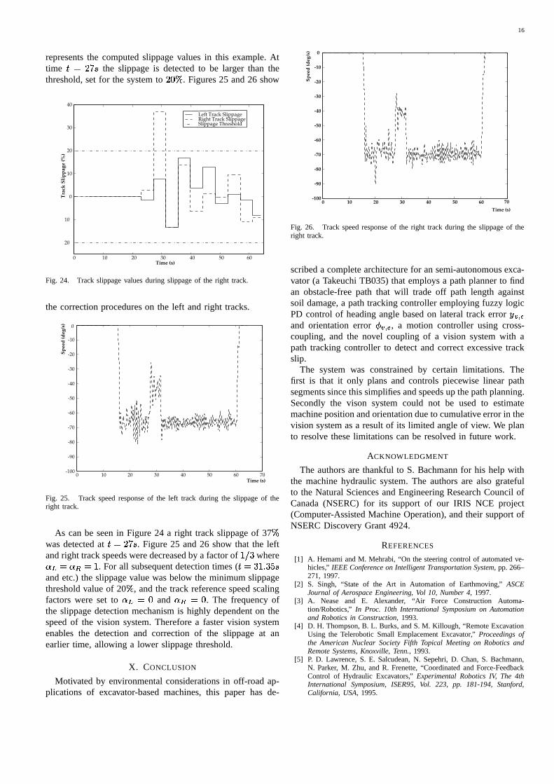
The ability of the path planner to integrate with the pathtracking controller was first evaluated. This experiment wascarried out on a flat concrete laboratory floor with a 5m by5m area marked off in 1m by 1m squares. Obstacles werelocated in some of the squares and the locations of these wereentered into the path planner. The path planner weight
���was
set to 0. A human interface allowed the operator to enter agoal position (x,y) and to observe the paths found by theplanner. The locations of two sets of obstacles and the pathsfound are shown in Figure 21. A calibrated camera placed
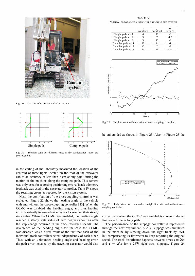
15
Camerasystem
Fig. 20. The Takeuchi TB035 tracked excavator.
Simple path Complex path
1
2
3
4
5
6
1
2
3
4
5
6
1 2 3 4 5 6 1 2 3 4 5 6
..
.
.....
.
.
..
x
x
x
x
Fig. 21. Solution paths for different cases of the configuration space andgoal positions.
in the ceiling of the laboratory measured the location of thecentroid of three lights located on the roof of the excavatorcab to an accuracy of less than 7 cm at any point during themotion of the machine along the complete path. This camerawas only used for reporting positioning errors. Track odometryfeedback was used in the excavator controller. Table IV showsthe resulting errors as reported by the vision system.
Next, the contribution of the cross-coupling controller wasevaluated. Figure 22 shows the heading angle of the vehiclewith and without the cross-coupling controller [43]. When theCCMC was disabled, the heading angle, and thus headingerror, constantly increased once the tracks reached their steadystate value. When the CCMC was enabled, the heading anglereached a steady state value of zero degrees about 4s afterthe step change occurred in the track reference speeds. Thedivergence of the heading angle for the case the CCMCwas disabled was a direct result of the fact that each of theindividual track controllers acted independently of each other.Thus, with an unbounded heading angle and heading error,the path error incurred by the traveling excavator would also
TABLE IV
POSITION ERRORS MEASURED WHILE RUNNING THE SYSTEM.
x y�
error[cm] error[cm] error[� ]Simple path no. 1 4 10 -3Simple path no. 2 3 7 -1.5Simple path no. 3 5 10 -3
Complex path no. 1 12 14 -1Complex path no. 2 12 7 -3Complex path no. 3 10 15 -4.5
0 5 10 15 20 25 30-2
-1
0
1
2
3
4
5
Time (s)
Hea
ding
Ang
le E
rror
(deg
)
Without CC ControllerWith CC Controller
Fig. 22. Heading error with and without cross coupling controller.
be unbounded as shown in Figure 23. Also, in Figure 23 the
0.2 0.15 0.1 0.05 0 0.050
1
2
3
4
5
6
7
Y Distance (m)
X D
ista
nce
(m)
Without CC ControllerWith CC Controller
Fig. 23. Path driven for commanded straight line with and without crosscoupling controller.
correct path when the CCMC was enabled is shown in dottedline for a 7 meter long path.
The performance of the slippage controller is representedthrough the next experiment. A 25 � slippage was simulatedin the machine by slowing down the right track by 25 �but compensating its flowmeter to keep reporting the originalspeed. The track disturbance happens between times � � � � and � � � � for a 25 � right track slippage. Figure 24
16
represents the computed slippage values in this example. Attime � � � � the slippage is detected to be larger than thethreshold, set for the system to � � � . Figures 25 and 26 show
0 10 20 30 40 50 60
20
10
0
10
20
30
40
Time (s)
Tra
ck S
lipp
age
(%)
Left Track Slippage Right Track SlippageSlippage Threshold
Fig. 24. Track slippage values during slippage of the right track.
the correction procedures on the left and right tracks.
0 10 20 30 40 50 60 70-100
-90
-80
-70
-60
-50
-40
-30
-20
-10
Time (s)
Spee
d (d
eg/s
) 0
Fig. 25. Track speed response of the left track during the slippage of theright track.
As can be seen in Figure 24 a right track slippage of 37 �was detected at � � � � . Figure 25 and 26 show that the leftand right track speeds were decreased by a factor of
� & � where� � � � � � � . For all subsequent detection times (� � � � � � � and etc.) the slippage value was below the minimum slippagethreshold value of 20 � , and the track reference speed scalingfactors were set to � � � � and � � � � . The frequency ofthe slippage detection mechanism is highly dependent on thespeed of the vision system. Therefore a faster vision systemenables the detection and correction of the slippage at anearlier time, allowing a lower slippage threshold.
X. CONCLUSION
Motivated by environmental considerations in off-road ap-plications of excavator-based machines, this paper has de-
0 10 20 30 40 50 60-100
-90
-80
-70
-60
-50
-40
-30
-20
-10
0
Time (s)
Spee
d (d
eg/s
)
70
Fig. 26. Track speed response of the right track during the slippage of theright track.
scribed a complete architecture for an semi-autonomous exca-vator (a Takeuchi TB035) that employs a path planner to findan obstacle-free path that will trade off path length againstsoil damage, a path tracking controller employing fuzzy logicPD control of heading angle based on lateral track error
� � �and orientation error
��� � � , a motion controller using cross-coupling, and the novel coupling of a vision system with apath tracking controller to detect and correct excessive trackslip.
The system was constrained by certain limitations. Thefirst is that it only plans and controls piecewise linear pathsegments since this simplifies and speeds up the path planning.Secondly the vison system could not be used to estimatemachine position and orientation due to cumulative error in thevision system as a result of its limited angle of view. We planto resolve these limitations can be resolved in future work.
ACKNOWLEDGMENT
The authors are thankful to S. Bachmann for his help withthe machine hydraulic system. The authors are also gratefulto the Natural Sciences and Engineering Research Council ofCanada (NSERC) for its support of our IRIS NCE project(Computer-Assisted Machine Operation), and their support ofNSERC Discovery Grant 4924.
REFERENCES
[1] A. Hemami and M. Mehrabi, “On the steering control of automated ve-hicles,” IEEE Conference on Intelligent Transportation System, pp. 266–271, 1997.
[2] S. Singh, “State of the Art in Automation of Earthmoving,” ASCEJournal of Aerospace Engineering, Vol 10, Number 4, 1997.
[3] A. Nease and E. Alexander, “Air Force Construction Automa-tion/Robotics,” In Proc. 10th International Symposium on Automationand Robotics in Construction, 1993.
[4] D. H. Thompson, B. L. Burks, and S. M. Killough, “Remote ExcavationUsing the Telerobotic Small Emplacement Excavator,” Proceedings ofthe American Nuclear Society Fifth Topical Meeting on Robotics andRemote Systems, Knoxville, Tenn., 1993.
[5] P. D. Lawrence, S. E. Salcudean, N. Sepehri, D. Chan, S. Bachmann,N. Parker, M. Zhu, and R. Frenette, “Coordinated and Force-FeedbackControl of Hydraulic Excavators,” Experimental Robotics IV, The 4thInternational Symposium, ISER95, Vol. 223, pp. 181-194, Stanford,California, USA, 1995.
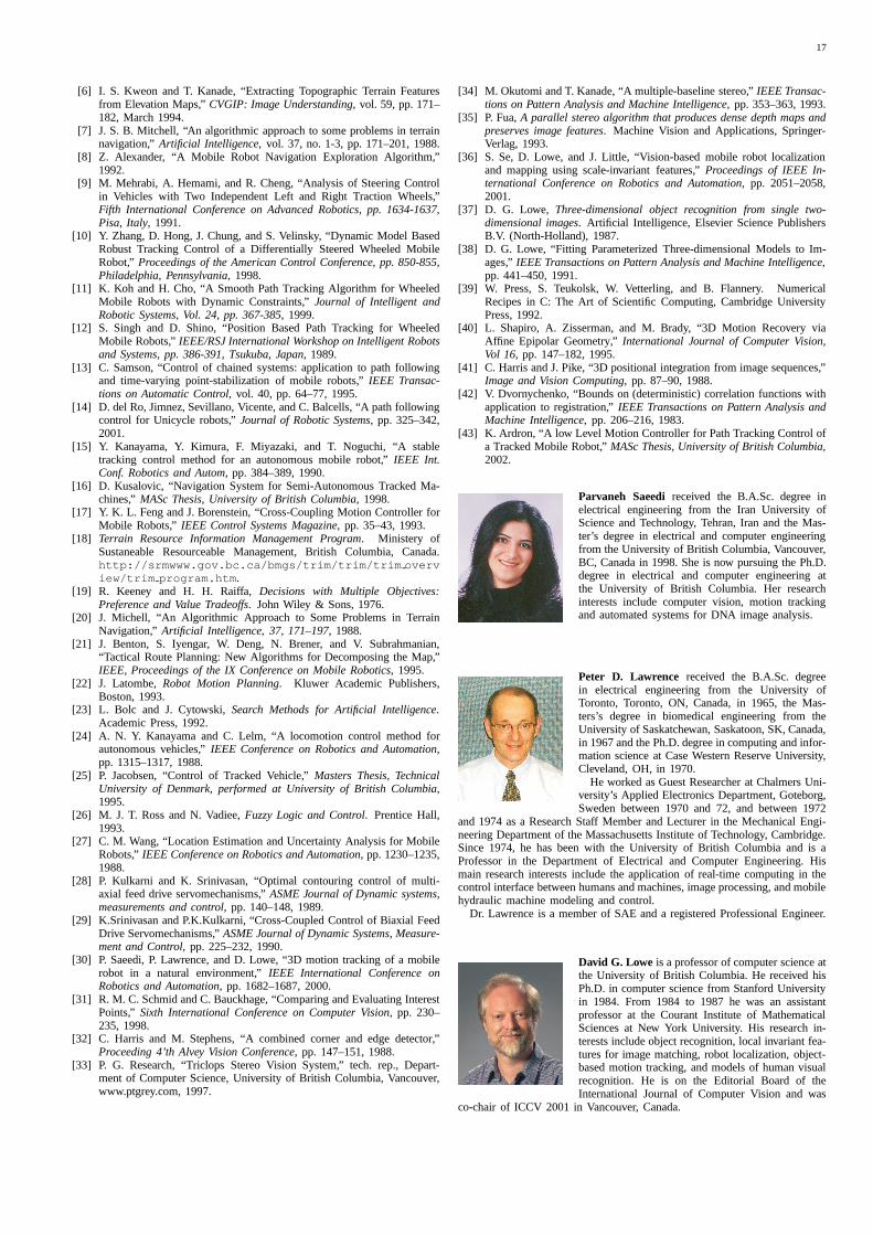
17
[6] I. S. Kweon and T. Kanade, “Extracting Topographic Terrain Featuresfrom Elevation Maps,” CVGIP: Image Understanding, vol. 59, pp. 171–182, March 1994.
[7] J. S. B. Mitchell, “An algorithmic approach to some problems in terrainnavigation,” Artificial Intelligence, vol. 37, no. 1-3, pp. 171–201, 1988.
[8] Z. Alexander, “A Mobile Robot Navigation Exploration Algorithm,”1992.
[9] M. Mehrabi, A. Hemami, and R. Cheng, “Analysis of Steering Controlin Vehicles with Two Independent Left and Right Traction Wheels,”Fifth International Conference on Advanced Robotics, pp. 1634-1637,Pisa, Italy, 1991.
[10] Y. Zhang, D. Hong, J. Chung, and S. Velinsky, “Dynamic Model BasedRobust Tracking Control of a Differentially Steered Wheeled MobileRobot,” Proceedings of the American Control Conference, pp. 850-855,Philadelphia, Pennsylvania, 1998.
[11] K. Koh and H. Cho, “A Smooth Path Tracking Algorithm for WheeledMobile Robots with Dynamic Constraints,” Journal of Intelligent andRobotic Systems, Vol. 24, pp. 367-385, 1999.
[12] S. Singh and D. Shino, “Position Based Path Tracking for WheeledMobile Robots,” IEEE/RSJ International Workshop on Intelligent Robotsand Systems, pp. 386-391, Tsukuba, Japan, 1989.
[13] C. Samson, “Control of chained systems: application to path followingand time-varying point-stabilization of mobile robots,” IEEE Transac-tions on Automatic Control, vol. 40, pp. 64–77, 1995.
[14] D. del Ro, Jimnez, Sevillano, Vicente, and C. Balcells, “A path followingcontrol for Unicycle robots,” Journal of Robotic Systems, pp. 325–342,2001.
[15] Y. Kanayama, Y. Kimura, F. Miyazaki, and T. Noguchi, “A stabletracking control method for an autonomous mobile robot,” IEEE Int.Conf. Robotics and Autom, pp. 384–389, 1990.
[16] D. Kusalovic, “Navigation System for Semi-Autonomous Tracked Ma-chines,” MASc Thesis, University of British Columbia, 1998.
[17] Y. K. L. Feng and J. Borenstein, “Cross-Coupling Motion Controller forMobile Robots,” IEEE Control Systems Magazine, pp. 35–43, 1993.
[18] Terrain Resource Information Management Program. Ministery ofSustaneable Resourceable Management, British Columbia, Canada.http://srmwww.gov.bc.ca/bmgs/trim/trim/trim overview/trim program.htm.
[19] R. Keeney and H. H. Raiffa, Decisions with Multiple Objectives:Preference and Value Tradeoffs. John Wiley & Sons, 1976.
[20] J. Michell, “An Algorithmic Approach to Some Problems in TerrainNavigation,” Artificial Intelligence, 37, 171–197, 1988.
[21] J. Benton, S. Iyengar, W. Deng, N. Brener, and V. Subrahmanian,“Tactical Route Planning: New Algorithms for Decomposing the Map,”IEEE, Proceedings of the IX Conference on Mobile Robotics, 1995.
[22] J. Latombe, Robot Motion Planning. Kluwer Academic Publishers,Boston, 1993.
[23] L. Bolc and J. Cytowski, Search Methods for Artificial Intelligence.Academic Press, 1992.
[24] A. N. Y. Kanayama and C. Lelm, “A locomotion control method forautonomous vehicles,” IEEE Conference on Robotics and Automation,pp. 1315–1317, 1988.
[25] P. Jacobsen, “Control of Tracked Vehicle,” Masters Thesis, TechnicalUniversity of Denmark, performed at University of British Columbia,1995.
[26] M. J. T. Ross and N. Vadiee, Fuzzy Logic and Control. Prentice Hall,1993.
[27] C. M. Wang, “Location Estimation and Uncertainty Analysis for MobileRobots,” IEEE Conference on Robotics and Automation, pp. 1230–1235,1988.
[28] P. Kulkarni and K. Srinivasan, “Optimal contouring control of multi-axial feed drive servomechanisms,” ASME Journal of Dynamic systems,measurements and control, pp. 140–148, 1989.
[29] K.Srinivasan and P.K.Kulkarni, “Cross-Coupled Control of Biaxial FeedDrive Servomechanisms,” ASME Journal of Dynamic Systems, Measure-ment and Control, pp. 225–232, 1990.
[30] P. Saeedi, P. Lawrence, and D. Lowe, “3D motion tracking of a mobilerobot in a natural environment,” IEEE International Conference onRobotics and Automation, pp. 1682–1687, 2000.
[31] R. M. C. Schmid and C. Bauckhage, “Comparing and Evaluating InterestPoints,” Sixth International Conference on Computer Vision, pp. 230–235, 1998.
[32] C. Harris and M. Stephens, “A combined corner and edge detector,”Proceeding 4’th Alvey Vision Conference, pp. 147–151, 1988.
[33] P. G. Research, “Triclops Stereo Vision System,” tech. rep., Depart-ment of Computer Science, University of British Columbia, Vancouver,www.ptgrey.com, 1997.
[34] M. Okutomi and T. Kanade, “A multiple-baseline stereo,” IEEE Transac-tions on Pattern Analysis and Machine Intelligence, pp. 353–363, 1993.
[35] P. Fua, A parallel stereo algorithm that produces dense depth maps andpreserves image features. Machine Vision and Applications, Springer-Verlag, 1993.
[36] S. Se, D. Lowe, and J. Little, “Vision-based mobile robot localizationand mapping using scale-invariant features,” Proceedings of IEEE In-ternational Conference on Robotics and Automation, pp. 2051–2058,2001.
[37] D. G. Lowe, Three-dimensional object recognition from single two-dimensional images. Artificial Intelligence, Elsevier Science PublishersB.V. (North-Holland), 1987.
[38] D. G. Lowe, “Fitting Parameterized Three-dimensional Models to Im-ages,” IEEE Transactions on Pattern Analysis and Machine Intelligence,pp. 441–450, 1991.
[39] W. Press, S. Teukolsk, W. Vetterling, and B. Flannery. NumericalRecipes in C: The Art of Scientific Computing, Cambridge UniversityPress, 1992.
[40] L. Shapiro, A. Zisserman, and M. Brady, “3D Motion Recovery viaAffine Epipolar Geometry,” International Journal of Computer Vision,Vol 16, pp. 147–182, 1995.
[41] C. Harris and J. Pike, “3D positional integration from image sequences,”Image and Vision Computing, pp. 87–90, 1988.
[42] V. Dvornychenko, “Bounds on (deterministic) correlation functions withapplication to registration,” IEEE Transactions on Pattern Analysis andMachine Intelligence, pp. 206–216, 1983.
[43] K. Ardron, “A low Level Motion Controller for Path Tracking Control ofa Tracked Mobile Robot,” MASc Thesis, University of British Columbia,2002.
Parvaneh Saeedi received the B.A.Sc. degree inelectrical engineering from the Iran University ofScience and Technology, Tehran, Iran and the Mas-ter’s degree in electrical and computer engineeringfrom the University of British Columbia, Vancouver,BC, Canada in 1998. She is now pursuing the Ph.D.degree in electrical and computer engineering atthe University of British Columbia. Her researchinterests include computer vision, motion trackingand automated systems for DNA image analysis.
Peter D. Lawrence received the B.A.Sc. degreein electrical engineering from the University ofToronto, Toronto, ON, Canada, in 1965, the Mas-ters’s degree in biomedical engineering from theUniversity of Saskatchewan, Saskatoon, SK, Canada,in 1967 and the Ph.D. degree in computing and infor-mation science at Case Western Reserve University,Cleveland, OH, in 1970.
He worked as Guest Researcher at Chalmers Uni-versity’s Applied Electronics Department, Goteborg,Sweden between 1970 and 72, and between 1972
and 1974 as a Research Staff Member and Lecturer in the Mechanical Engi-neering Department of the Massachusetts Institute of Technology, Cambridge.Since 1974, he has been with the University of British Columbia and is aProfessor in the Department of Electrical and Computer Engineering. Hismain research interests include the application of real-time computing in thecontrol interface between humans and machines, image processing, and mobilehydraulic machine modeling and control.
Dr. Lawrence is a member of SAE and a registered Professional Engineer.
David G. Lowe is a professor of computer science atthe University of British Columbia. He received hisPh.D. in computer science from Stanford Universityin 1984. From 1984 to 1987 he was an assistantprofessor at the Courant Institute of MathematicalSciences at New York University. His research in-terests include object recognition, local invariant fea-tures for image matching, robot localization, object-based motion tracking, and models of human visualrecognition. He is on the Editorial Board of theInternational Journal of Computer Vision and was
co-chair of ICCV 2001 in Vancouver, Canada.
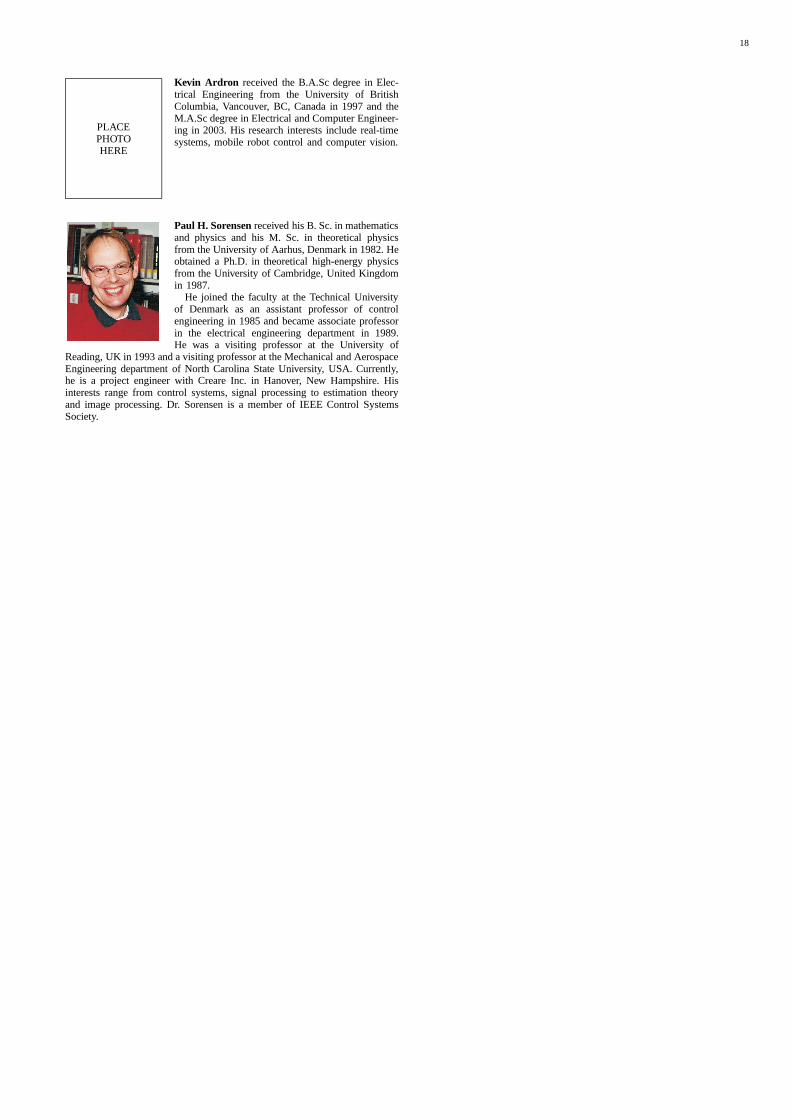
18
PLACEPHOTOHERE
Kevin Ardron received the B.A.Sc degree in Elec-trical Engineering from the University of BritishColumbia, Vancouver, BC, Canada in 1997 and theM.A.Sc degree in Electrical and Computer Engineer-ing in 2003. His research interests include real-timesystems, mobile robot control and computer vision.
Paul H. Sorensen received his B. Sc. in mathematicsand physics and his M. Sc. in theoretical physicsfrom the University of Aarhus, Denmark in 1982. Heobtained a Ph.D. in theoretical high-energy physicsfrom the University of Cambridge, United Kingdomin 1987.
He joined the faculty at the Technical Universityof Denmark as an assistant professor of controlengineering in 1985 and became associate professorin the electrical engineering department in 1989.He was a visiting professor at the University of
Reading, UK in 1993 and a visiting professor at the Mechanical and AerospaceEngineering department of North Carolina State University, USA. Currently,he is a project engineer with Creare Inc. in Hanover, New Hampshire. Hisinterests range from control systems, signal processing to estimation theoryand image processing. Dr. Sorensen is a member of IEEE Control SystemsSociety.