An Assessment of Factors Affecting the Spatial ...

An Assessment of Factors Affecting the Spatial Distribution of Audubon’s Shearwater (Puffinus

l. lherminieri) throughout the Caribbean

by

Copyright 2015

William Edward Chatfield-Taylor

Submitted to the graduate degree program in Geography and the Graduate Faculty of the

University of Kansas in partial fulfillment of the requirements for the degree of Masters of

Science

________________________________

Chairperson William Johnson

________________________________

Co-Chair Johannes Feddema

________________________________

Adrian Delnevo

Date Defended: April 27, 2015

ii

The Thesis Committee for William Edward Chatfield-Taylor

Certifies that this is the approved version of the following thesis


l. lherminieri) throughout the Caribbean

_____________________________

Chairperson William Johnson

_____________________________

Co-Chair Johannes Feddema

Date approved: April 4, 2015

iii

Abstract:

This study aims to better understand the factors that contribute to Audubon’s Shearwater

(Puffinus l. lherminieri) nesting sites on islands across the Caribbean region. Using locational

presence and absence data of their breeding colonies a Geographical Information System (GIS)

is used to determine the proximity and presence of a variety of marine (SST, bathymetry and

derived bathymetry data) and terrestrial (elevation derived statistics) environmental variables that

may influence nesting locations. For each location in the dataset, a set of nearshore (within 50

km) and offshore (50 and 300 km) metrics are calculated. Each selected variable is tested for

statistical significance both in the nearshore and offshore locations. Logistic regression analysis

is used to predict the presence and absence of sites. It is determined that a combination of

bathymetry, sea surface temperature (SST), and ocean front proxies are the best variables for

predicatively modeling Audubon’s Shearwater nesting locations. A different subset of SST

metrics and SST front proxies predict colony presence and absence when considering the

offshore data. Both models have a predicative accuracy of 62.72%, with a degree of uncertainty

arising from the quality of the presence and absence data. It is likely the relative success of both

nearshore and offshore logistic regression analyses is linked to the respective, and differing,

ecological roles that males and females play in the pre-laying exodus in this species. Despite the

difficulty of detecting true absence data for this study, the results suggest that there is a great

need to better understand the differential sex roles of Audubon’s Shearwater and their breeding

behavior to assist in future conservations efforts of the species.

iv

Acknowledgments:

I would like to thank Adrian Delnevo for the inspiration to take on this project and the

encouragement to see it through. I would also like to thank Johannes Feddema and William

Johnson for their guidance and support as advisors. I would like to thank the Dutch Caribbean

Nature Alliance (DCNA) for financial assistance and support. Other individuals who helped

make this research possible with their insight are Sarah Gille, Daphne Fautin, and Debi

Shearwater. I would also like to thank all those who have contributed observational data to the

Audubon’s Shearwater information database: without their work, this research never would have

been possible.

v

Table of Contents

Abstract…………………………………………………………………………………………..iii

Acknowledgments……………………………………………………………………………......iv

Preface............................................................................................................................................1

Preface 1.1: Research History.............................................................................................1

Preface 1.2: Organization of the Paper...............................................................................2


l. lherminieri) Throughout the Caribbean.......................................................................................4

Introduction....................................................................................................................................4

Methods..........................................................................................................................................7

Methods 1.1: Data Collection and Processing....................................................................7

Methods 1.2: Method of analysis........................................................................................9

Methods 1.3: Statistical Analysis.......................................................................................11

Methods 1.4: Puffinus l. loyemilleri analysis.....................................................................13

Results...........................................................................................................................................14

Discussion......................................................................................................................................18

Discussion 1.1: Pre-laying Exodus....................................................................................18

Discussion 1.2: Sources of Error and Potential Changes in Methodology........................20

vi

Discussion 1.3: Puffinus l. loyemilleri Analysis................................................................22

Discussion 1.4: Use of the Study in General Conservation...............................................23

Conclusion.....................................................................................................................................25

Conclusion 1.1: Research in Retrospect............................................................................25

Conclusion 1.2: Future Research.......................................................................................26

Literature Cited..............................................................................................................................31

Appendix A: Tables.......................................................................................................................37

Appendix B: Figures......................................................................................................................44

Appendix C: Main Shearwater Shapefile Format..........................................................................53

Appendix D: Puffinus l. loyemilleri Shapefile...............................................................................56

1

Preface

Preface 1.1: Research History

The genesis of this project has its roots in an attempt to identify suitable breeding habitat

for Audubon’s Shearwater on the island of Saba in the Netherlands Antilles. The goal of the

project as it was originally conceived was to determine if Audubon’s Shearwater habitat could be

mapped across the island using surface metrics in a Geographic Information System (GIS). A

combination of habitat information for breeding Audubon’s Shearwaters was to be collected,

based on a selection of terrestrial variables, including slope, elevation, aspect, and percent

vegetation cover around the breeding sites. Although Audubon’s Shearwaters are known to breed

on Saba (Collier et al. 2002), this initial approach was determined to be unfeasible because no

burrows of breeding Audubon’s Shearwaters were found to determine optimal nesting

conditions. Further work to find nesting sites was deemed too difficult for this project due to the

inaccessibility of Saba’s cliffs for detailed exploration. The cliffs of Saba are composed of

fragile, highly friable rock that cannot be safely traversed even with appropriate climbing gear

(A. J. Delnevo, personal communication).

After it was determined that finding individual nests would prove to be impossible, the

project was changed to characterizing the landscape of the areas in which Audubon’s

Shearwaters were known to be breeding locations that had been identified by the presence of the

birds’ nocturnal flight calls. The physical characteristics of these sites were going to be analyzed

using GIS and compared to the characteristics of sites where shearwaters were not known to be

nesting. A statistical analysis was intended to identify the values in terms of slope and aspect that

would limit the breeding locations for Audubon’s Shearwater. However, after an initial review of

2

the literature, an inherent flaw was discovered in this research design. While Audubon’s

Shearwaters are almost exclusively cavity nesters (Mackin 2004; Snow 1965; Trimm 2004) they

do not use cliffs exclusively. While they do nest in cliffs in some regions, such as the Galapagos

and Réunion Island (Brentagnolle et al. 2000; Snow 1965), elsewhere they nest on flat ground

under boulders and vegetation or even in burrows within the sand (Schreiber and Lee 2002;

Trimm 2004).

Following these preliminary explorations, it was hypothesized that a more probable cause

driving their breeding site distribution was the availability of food sources. Due to Audubon’s

Shearwater’s practice of feeding exclusively on marine prey, it was determined that oceanic

variables that could affect prey distribution would be more promising for analysis. It was also

determined that Saba, due to its small size, did not represent a sufficiently large sample for a

productive analysis. To address this issue, the problem of breeding site selection was expanded

to include all available Audubon’s Shearwater breeding site data for the entire Caribbean. With

the inclusion of multiple variables and a binomial presence/absence data structure, it was decided

that the best method of analysis to use was multivariate binomial logistic regression. As the

research progressed, complexity of the analysis changed and was then modified to the point

when it emerged in its final form as presented in this thesis.

Preface 1.2: Organization of the Paper

Following this introduction to the thesis, the second section is formatted as a manuscript

to be submitted to a journal. The introduction provides the basic review of literature for the

article being submitted to the journal Ecological Applications, published by the Ecological

Society of America. It provides an overview of the previous work on Audubon’s Shearwater in

3

the Caribbean and seabird modeling in general. The introduction concludes by setting out the

individual goals of the paper its primary conclusions. The methods section is geared primarily to

a readership comprised of biologists (which is reflective of the journal), and provides only an

outline of the GIS methodology. It emphasis is however, on the statistical methods employed in

the research. The results section contains appropriate tables and nine figures, one of which shows

the results of one of the GIS methodologies, and eight maps illustrating results of the different

analyses that were performed. The discussion focuses primarily on the role of what is known as

the pre-laying exodus as the likely causative force behind the patterns observed in the results, as

well as the role of the study in future conservation efforts for the species. A post-manuscript

conclusion section expands on the major changes to the methodology in light of what is now

suspected about the role of the pre-laying exodus. It also outlines three further projects that could

be undertaken as an extension and continuation of the research conducted.

4

An Assessment of Factors Affecting the Spatial Distribution of Audubon’s Shearwater

(Puffinus l. lherminieri) Throughout the Caribbean

Introduction

Audubon’s Shearwater (Puffinus lherminieri, Lesson 1839) is a small seabird with a body

that is black above and pure white below, weighing between 180g-230g, and about 30cm in

length with a wingspan of about 70cm and pantropical distribution (Howell 2012). Within the

Caribbean, there is an estimated population of 8,000 individuals, comprising approximately

3,000-5,000 nesting pairs which represents a decline in number from the beginning of the 20th

century (BirdLife 2008; Schreiber and Lee 2002; USFWS 2011). Included within the Caribbean

population are the nominate P. l. lherminieri and the nearly extinct P. l. loyemilleri subspecies

(Balloffet et al. 2006). In order to aid in future conservation efforts, a more thorough

understanding of the oceanographic and terrestrial variables which drive the large-scale breeding

distribution of this species in the Caribbean is required.

Relatively little work on Audubon’s Shearwater has been conducted in the Caribbean in

the context of understanding the spatial nature of their breeding distribution. The primary work

on this species in the Caribbean has focused on their breeding ecology and behavior at single

colonies in the Bahamas (Mackin 2004; Mackin 2009; Trimm 2004; Trimm and Hayes 2005).

Recently, ecological niche models were used to identify possible breeding colonies of

Audubon’s Shearwater off the Brazilian coast (Lopes et al. 2014). This study analyzed several

oceanographic variables, including bathymetry and sea surface temperature (SST), both of which

were used in this study. The investigators employed the Maxent algorithm to produce an

ecological niche model using a small sample size from a limited geographic area (Lopes et al.

2014).

5

Oceanic variables have been utilized in a wide variety of studies that model seabirds. Due

to their effects on concentrating seabirds, sea surface temperature and bathymetric metrics have

been used to identify marine ‘hot spots’ off California (Nur et al. 2011). Chlorophyll

concentrations have shown to be important in affecting the foraging ecology of multiple pelagic

seabird species (Vilchis et al. 2006). Other combinations of these variables have been used to

explain seabird distributions during upwelling periods (Ainley et al. 2005), and to explain the

breeding distribution of multiple seabird species in the Northwest Atlantic (Huettmann and

Diamond 2001). Certain physical oceanographic data, such as isobaths, have been used for both

‘hot spot’ detection (Nur et al. 2011) and seabird distribution modeling in the South Pole (Ainley

et al. 1998). This study employs a new class of features- bathymetric breaks- for the purpose of

determining breeding distributions.

Rather than focusing on a small geographic area, this study uses breeding distribution

presence and absence data for the entire Caribbean (Bradley and Norton 2009). Using a GIS as

an organizing platform, potentially significant oceanographic and terrestrial variables that may

influence the breeding distribution of Audubon’s Shearwater are identified. Oceanographic

variables are selected to identify potential food resource areas that can sustain large bird

populations. The inclusion of terrestrial variables, particularly slope, is suggested by the presence

of several exceptionally large colonies of Audubon’s Shearwaters nesting in cliff cavities on

Saba in the Netherlands Antilles, Réunion Island in the Indian Ocean, and on the Galapagos

Islands (Brentagnolle et al. 2000; Snow 1965). The subset of variables that exhibit statistical

significance at differentiating presence from absence sites are used in logistic regression to

6

determine which exact combination of variables yields the best predicative model of Audubon’s

Shearwater nesting sites.

Because Audubon’s Shearwaters are known to have extensive habitat ranges, the final

question this study aims to address is whether distance has a significant impact on breeding

locations. To address this question, the analysis divided ocean variables into two distinct zones

(Near and Pelagic) based on distance to presence and absence sites. In addition to assessing how

Audubon’s Shearwater use food resources during breeding, it may also reflect the sexual-

dimorphism inherent in the post-copulation mass emigration of females (and occasionally males)

from the breeding colony, known as the pre-laying exodus (Warham 1990). The zonal nature of

the analysis allows for some speculation as to which sex plays a more important role in

determining the breeding distribution of the birds.

7

Methods

Methods 1.1: Data Collection and Processing

Bird observational data.- Breeding presence information in the form of presence and

non-presence or absence are taken primarily from Bradley and Norton (2009), but also from A. J.

Delnevo, (unpublished data), Hodge (2011), and Levesque and Yésou (2005). Audubon’s

Shearwater ‘presence’ indicates that at least one nest was found in at least one year. A total of 94

Audubon’s Shearwater ‘presence’ sites were identified and mapped in a GIS. The ‘absence’ sites

used in this study comprised a subset of those presented in Bradley and Norton (2009).

‘Absence’ sites are those locations where field surveys had been conducted in one or more years,

but where no Audubon’s Shearwaters were recorded. To create a balanced dataset without

‘absence’ prevalence, a subset dataset of the nearly 700 potential ‘absence’ sites in Bradley and

Norton (2009) is created. Whereas many locations lacking Audubon’s Shearwater in Bradley and

Norton (2009) listed only one to two pairs of breeding seabirds as being present, for this study

‘absence’ sites were chosen to be used only when relatively large numbers of breeding seabirds

were found. This approach indicated that the sites had a higher potential to be attractive to

Audubon’s Shearwaters as breeding sites due to the higher numbers of other breeding seabirds,

even though they were not recorded. A total of 75 ‘absence’ sites were generated from the

available data sources using this methodology.

All ‘presence’ and ‘absence’ sites were plotted in Google Earth (Google Inc., 2013) then

converted into an ArcGIS shapefile (ESRI ArcMap 10.1) for further manipulation. A database

was constructed within the GIS detailing numerous attributes about the sites, for example;

8

‘presence’ or ‘absence’ status, site name, months of incubation, and latitude and longitude of

site. Of particular interest were data pertaining to both the known or suspected egg incubation

period for each colony. For colonies where this information was missing and for ‘absence’ sites,

an estimation of that period was based on a nearby ‘presence’ sites with the information. For

colonies where only nestlings were found, the timing of the incubation was extrapolated using

the 49-day egg incubation period of Audubon’s Shearwater (Mackin 2004).

Environmental data.- To assist in identifying ocean resource sites for Audubon’s

Shearwater, monthly Chlorophyll-a (CHL) and sea surface temperature data from the

MODIS/AQUA satellite was acquired from the NASA Near Earth Observatory for each month

from January 2003 to December 2013. This data have a spatial resolution of 0.1 angular degrees

(this is approximately 11113m2 at the equator, but varies with latitude). The monthly data was

averaged over the 11-year period using ArcMap to create a single temporally averaged raster for

each month. Missing data, whether from sensor errors or cloud coverage was interpolated and

filled using a custom, temporal autocorrelation-based Python script (Python Software

Foundation, 2013) (Chatfield-Taylor and Li, in prep). All Python scripts used in this study were

written by the author and were GIS-based. All scripts made use of the ArcPy (ESRI) Python

module for performing GIS operations, and were executed using ArcMap. The bathymetric data

were obtained from the General Bathymetric Chart of the Oceans (GEBCO_08; 2014), which has

a spatial resolution of 30 arc-seconds (approximately 926m2 at the equator). The spatial extent of

the files is approximately from 97˚W to 56˚W and 32˚N to 4˚N.

Terrestrial elevation data were obtained from a void-filled version of NASA Shuttle

Radar Topographic Mission (SRTM) 90m2 Digital Elevation Model (DEM) dataset (Jarvis et al.

2008). The DEMs were converted into slope data using ArcMap, and both the DEM and slope

9

data were individually analyzed using custom Python scripts. Several other terrestrial variables

were considered initially, including percent vegetation cover and percent bare rock. However,

due to the practical challenges and cost of acquiring remotely sensed imagery at a sufficient

resolution, these variables were not considered in the analysis.

Precipitous drops in ocean floor depth and steep slope gradients, such as isobaths or the

mapped extent of the Continental Shelf have been used as modeling variables in seabird studies

(Ainley et al. 1998; Nur et al. 2011). Isobaths and ocean topography were found to be highly

associated with and exhibiting a causal relationship with GIS-detected thermal SST fronts

(Valavanis et al. 2005). Birds often congregate at topographically defined ‘hotspots’ which are

often associated with SST gradients (Nur et al. 2011). For this study, a proxy raster was

generated to indicate areas where sharp drops in ocean floor depth could cause the formation of

topographically-induced SST fronts or upwelling sites that could be attractive to seabirds. To

accomplish this, a Python script was written which searched the GEBCO_08 raster for all

locations where there was a bathymetry change of at least 500’ (152.4m) between a central cell

and any of its surrounding 8 cells. The identified pixels constitute what is herien referred to as

‘bathymetric breaks’ (Figure 1), which illustrates how the methodology can be used to identify

known feeding grounds (Trimm 2004). Then using ArcMap, all the resulting bathymetric breaks

that had a bottom depth of more than 750’ (228.6m) were eliminated, a step performed to ensure

that only near surface breaks were included in the analysis. These areas are likely to be

associated with surface SST front formation and upwelling areas that affect surface conditions.

Methods 1.2: Method of analysis

10

Zonal division of the area of analysis.- Analysis of the area surrounding each presence or

absence site was divided into two distinct zones: a Near Zone and a Pelagic Zone. The Near

Zone constituted a circular area around each site with a radius of 50km. The Pelagic Zone was a

ring that extended from 50km to 300km from the center of each site (Figure 2). Analysis of

ocean properties within each is intended to ascertain whether or not the distance to food sources

has a deterministic effect on the breeding distribution of Audubon’s Shearwater. The outer limit

of the Pelagic Zone is based on the approximate foraging radius of the closely related Manx

Shearwaters (Puffinus puffinus) from Skomer Island in Wales during their nesting period

(Guilford et al. 2008). Audubon’s Shearwater and Manx Shearwater share a broadly similar

breeding ecology (Brooke 1990).

Python scripts are used to derive a number of metrics to summarize conditions within

each zone for each ‘presence’ and absence site. For SST, CHL and bathymetry, the following

metrics were computed: minimum, maximum, mean, median, standard deviation, and mean

absolute difference (MAD) as a metric of variability (Equation 1), where x̄ is the mean value for

each data set, xi is each individual value of x, and n is the total number of data points.

Equation 1: ∑ |�̅�−𝑥𝑖|𝑛𝑖=1

𝑛

For the bathymetric breaks data, the following metrics were calculated: number of bathymetric

breaks per zone, total size of the breaks (in pixels), and the distance from each colony to the

nearest break (minimum distance). Terrestrial slope and elevation were not analyzed by zone,

though similar metrics to SST, CHL, and bathymetry were calculated for each of those variables.

Since SST and CHL data have a temporal component, zonal analysis is only conducted on

months during which birds are incubating (or are most likely be incubating for absence data) at a

11

given site. Once all the analyses had been performed, a Python script was run that averaged the

data for the analyzed time span at each site, resulting in a single mean value.

Methods 1.3: Statistical Analysis

Identifying statistically significant variables.- Using a combination of Minitab 16

(Minitab Inc., 2013) and the SciPy module of Python (SciPy.org, 2014), means or medians of the

‘presence’ and ‘absence’ data were compared using two-sampled t-tests or Mann-Whitney U

Tests. Variables with means (or medians) that are statistically significantly different between the

two groups were selected for use in the logistic regression model.

Selection of variables for logistic regression.- Multivariate binomial logistic regression

from the Generalized Linear Model set of equations is a robust method of analysis and is often

used in modeling presence and absence data (Huettmann and Diamond 2001; Loiselle et al.

2003). The logistic regression approach employed in this study is implemented using RStudio

(RStudio, 2013). Initially, for each zone a total of seven variable metrics were selected and added

to the regression equation for subsequent analysis. Results of the model were analyzed using the

methodology of Barve and Slocum (2014). The code sorts predicted values into a contingency

table based on whether or not the probability that the dependent variable is equal to 1 was greater

or less than a cutoff of 0.5 (generating a predicted presence or absence) and comparing them to

the actual presence and absence values of the dependent variable. Variables are subtracted and

added until a model is reached that maximizes correct predictions while minimizing Type-I and

Type-II errors (false-positives and false-negatives, respectively).

Sensitivity analysis.- The initial logistic regression analysis uses a cutoff probability value

of 0.5 to construct the contingency tables showing the accuracy of the model. A sensitivity

12

analysis was conducted by running the same code with different cutoff values, from 0.25 to 0.75.

The total number of actual predicted presences and actual predicted absences are each plotted as

a percentage of the total number of presences and absences, resulting in two data sets. Linear

regression was conducted on each data set, and the ‘x’ value of the intersection of the two

equations was calculated. This value ‘x’ represents the approximate cutoff probability value

where the columns of the contingency table add up to the original number of presences and

absences while maximizing the ability of the model to correctly predict values. An optimized

sensitivity probability was obtained for each zone using this method.

Accuracy analysis by geographic region.- The accuracies for the logistic regression

equations for each zone were also calculated based on the two main geographic regions in the

Caribbean: the Greater Antilles and Lesser Antilles. Using ArcMap, the main spatial data file

containing the results of the logistic regression analyses and their predictions was divided into

these two regions. Using these geographically divided data files, regional model accuracies were

calculated based on contingency tables that sorted correct versus incorrect predictions.

Model validation.- Cross-validation with replication was performed on the Near Zone

logistic regression model as a standard form of model validation (Mertler and Vannatta 2013). A

random subset of five presence sites and five absence sites was removed from the model and the

logistic regression was re-run with the remaining data. The resulting equation was then used to

calculate the probabilities for the ten removed sites. Using the optimized probability derived

from the sensitivity analysis as a cutoff, the ten sites were sorted into correct or incorrect

predictions. The predicative accuracy was then calculated for the ten sites as a percentage. This

procedure was repeated 25 times. To test whether the cross-validation results deviated from the

13

overall model accuracy, a one-sample t-test was performed, testing the group mean against the

overall model accuracy.

Methods 1.4: Puffinus l. loyemilleri analysis

Analysis set-up.- GIS data file was constructed of nine sites where P. l. loyemilleri could

be potentially breeding using information gathered from multiple sources, including A. J.

Delnevo, (personal communication), Bradley and Norton (2009), and Croxall et al. (1984). The

sites were selected based on how recently they had been surveyed (if at all), their proximity to

known or former breeding sites for P. l. loyemilleri, and the suitability of the habitat. Using the

methodology set out in the earlier sections of this paper, the Near and Pelagic Zone analyses

were run on all nine sites. The resulting data were then entered into the Near and Pelagic Zone

logistic regression equations. The probabilities were then sorted as predicted presences and

absences, and then the sites were ranked based on whether both were predicted as a presence, if

only one zone predicted a presence, or if both predicted an absence. Within these categories, the

results were ranked by averaging the actual probabilities generated by the logistic regression

equations.

14

Results

Statistically significant variables.- Of the four oceanographic variables tested (SST,

CHL, bathymetry, and bathymetric breaks), at least one metric for each variable showed

statistical significance at an alpha level of 0.05 (Table 1). For the Near Zone, the variables and

metrics that showed statistical significance were Bathymetric Mean and Median, CHL Maximum

and Standard Deviation, SST Maximum, Number of Bathymetric Breaks, and Size of

Bathymetric Breaks. For the Pelagic Zone of analysis, Bathymetric Mean, Median, and Standard

Deviation, CHL Maximum, and SST Maximum were statistically significant. The Minimum

Distance from a bathymetric break to a site is zone independent and also reported the highest

level of statistical significance, with p-value=0.00034, and a difference in the medians of the two

groups of 0.077 angular degrees (approximately 8500m at the equator). A comparison between

the means (or medians) of the remaining presence and absence groups for the variables and

metrics tested is also related in Table 1. There were no statistically significant metrics for the

terrestrial variables (results not shown).

Selection of variables for logistic regression.- Due to the Near Zone presenting a larger

number of variables that were statistically significant, the variables selected for logistic

regression came from a subset of those variables. From the variable of bathymetric depth, the

metric of Mean Bathymetry was chosen due to its lower p-value than Bathymetric Median. The

single metric of CHL Maximum was selected, as it was the only metric of CHL that showed

statistical significance. From SST, the Maximum and Mean metrics were selected. Mean SST

was selected despite a non-significant (though low) p-value, due to inclusion of multiple SST

15

metrics in some studies (for example Huettmann and Diamond 2001). All three metrics for

bathymetric breaks were also included, for a total of four variables and seven metrics.

Multivariate logistic regression results.- The Near Zone logistic regression analysis

yielded an equation with four different variables (Table 2): Bathymetric Mean, SST Maximum,

Size of Bathymetric Breaks, and Minimum Distance to Bathymetric Breaks. Results of the

sensitivity analysis indicated a probability cutoff of 0.54, and actual manipulation showed that a

probability value of 0.53 yielded a model that had the greatest predicative accuracy for the Near

Zone (Table 3). The model was able to predict 62 presences and 44 absences correctly, for a

model accuracy of 62.72%. The results of the Near Zone analysis have been visualized in

Figures 3 through 5.

Results for the Pelagic Zone logistic regression analysis also yielded a four-variable

equation (Table 4). Variables that provided the best predicative model were SST Maximum, SST

Mean, Size of Bathymetric Breaks, and Minimum Distance to Bathymetric Breaks. The

sensitivity analysis provided a probability cutoff value of 0.56, which resulted in contingency

table with the highest predicative accuracy for the Pelagic Zone (Table 5). The model predicted

63 presences and 43 absences correctly, for a model accuracy of 62.72%. Results of the Pelagic

Zone are mapped in Figures 6 and 7.

In an attempt to discern any geographic patterns that might indicate where the models

differ in their predicative results, Figure 8 maps the predicted results of the two zones against

each other. One pattern that does emerge is that in the Greater Antilles, where the models

generated for both zones yield predicted results that are very similar, particularly in the Bahamas.

However, within the Lesser Antilles, the predictions of the two models differ considerably. Table

16

6 provides a contingency table to demonstrate how accurately each model performed with

respect to the other: the predictions of the two models coincided 81.07% of the time.

Geographically, in the Greater Antilles, the models coincided 82.17% of the time, while in the

Lesser Antilles they coincided 72.05% of the time. The accuracy of the two models was also

greater on average in the Greater Antilles, with the Near Zone model performing with an

accuracy of 68.31% and the Pelagic Zone performing with an accuracy of 65.34%. In the Lesser

Antilles, the Near Zone model showed an accuracy of 52.94% while the Pelagic Zone model

demonstrated an accuracy of 58.82%.

Model validation results.- The results of the replicated cross-validation of the Near Zone

logistic model did not differ statistically from the overall model accuracy of 62.72%. A one-

sample t-test performed on the pooled results of 25 replicates compared the mean of the group to

the overall model accuracy of 62.72%. The pooled results had a mean of 59.20% ±17.54% with

t=-1.00, df=24, p=0.326. The logistic regression model appears to be fairly robust when

subjected to cross-validation.

Puffinus l. loyemilleri analysis results.- Of the nine potential breeding sites for P. l.

loyemilleri, three were predicted to be suitable by the statistical analysis conducted in this study.

Of the three, Las Tortuguillas were predicted to be presences by both the Near and Pelagic Zone

logistic regression equations using the optimized probability values as the cut-offs. Of the

remaining two sites, Bubies Bajo, on the La Roques island chain was predicted by the Pelagic

Zone equation as a presence with a probability of approximately 65.5%. Klein Curaçao was

predicted by the Near Zone to be a presence with a probability of approximately 55.7%. Of the

remaining the sites, the probabilities were averaged and used as a metric to rank the islands in

order of likelihood that the loyemilleri subspecies breeds there. Logistic regression probabilities

17

are an ideal metric for this, as the value is actually the probability that outcome is “1” or a

presence. Islote Sucre off Northern Columbia had the highest mean probability of the remaining

sites, nearing 50%, while Monjes del Sur from the Los Monjes island group off the

Columbian/Venezuelan border had the lowest probability of approximately 15%. Full results of

the analysis of potential breeding sites for P. l. loyemilleri are depicted in Table 7. A map of the

resulting predictions is given in Figure 9.

18

Discussion

Discussion 1.1: Pre-laying Exodus

Nesting locations for Audubon’s Shearwater were analyzed throughout the Caribbean in

order to determine which factors likely contribute most to their breeding site distribution. The

measured variables were then used in logistic regression in order to determine exactly which

subset worked together to create the best predicative model, and to determine which zone of

analysis would do a better job of predicting this distribution. Results of the logistic regression

indicated a similar, though not exact subset of variables driving the breeding distribution in each

zone, and an equal predicative accuracy. However, the Near Zone had a total of seven different

statistically significant variable metrics, including one variable that was significant only for that

zone, compared to five variable metrics of the Pelagic Zone. This suggests that the Near Zone

likely has a slightly greater role in determining the breeding distribution of Audubon’s

Shearwater than the Pelagic Zone. This conclusion is reflected in the biology of the birds and

what these two zones could potentially be representing in terms of the breeding ecology of

Audubon’s Shearwater.

As of Bull’s (2006) work on the pre-laying exoduses of shearwater species, no new

information pertaining to the role of Audubon’s Shearwaters in this phenomenon had been

discovered to fill the gaps in of what was published by Warham (1990). However, in the

ecologically closely-related Manx Shearwater, there have been reports that only the females

undergo the exodus, while the males and non-breeders stay on the colony (Perrins and Brooke

1976; Warham 1990). Harris (1966) suggested that both sexes left the nesting colonies, but was

19

unable to comment on their movements after leaving their colony. If Audubon’s Shearwaters

display a similar pattern in pre-laying exodus ecology to Manx Shearwater as reported by

Warham (1990), the results of the zonal pattern of analysis could be explained by the two

different sexes operating in the two different zones.

Female birds on the pre-laying exodus could be using the Pelagic Zone (or possibly

greater distances) to search for food in order to gain sufficient nutrients for egg (particularly

yolk) development and thereby positively influence breeding success through egg size (Birkhead

and Delnevo 1987; Birkhead and Nettleship 1984; Delnevo 1990; Warham 1990). Studies of

other seabirds have shown that females may be avoiding nesting colonies to minimize forced

extra-pair copulations (EPC’s) (Birkhead et al. 1985; Birkhead and Delnevo 1987). Whereas

males likely stay close to shore, using the Near Zone for daily foraging in order defend their nest

site, be present to copulate with their returning female, and obtain EPC’s with visiting females

(Birkhead et al. 1985, Birkhead and Delnevo 1987, Delnevo 1990).

A similar nest guarding behavioral pattern of the males was observed in another

shearwater species, the Pintado Petrel (Daption capensis) (Pinder 1966). If the males are

constrained to stay close to shore to visit and guard the nests, while the females can range longer

distances, it would offer a possible explanation why a male-driven Near Zone appears to be more

important. This is supported by looking at the greater number of variables that are statistically

significant in the Near Zone when compared to the Pelagic Zone. However, because the tasks of

both the male and female are important, each zone of analysis can be used effectively as a

predicative model via logistic regression. The two equations likely describe different oceanic

ecosystems, both of which deal with variables that are important to the birds’ prey concentration

(Nur et al. 2011; Reese et al. 2011; Vilchis et al. 2006). Despite the temporal analysis not being

20

conducted in concert with the pre-laying exodus period, the conclusions drawn here are not

invalid. It is likely that the signal shown by SST in this study is similar but weaker than it would

have been had it been analyzed during the pre-laying exodus period.

Discussion 1.2: Sources of Error and Potential Changes in Methodology

After probability value optimization, both models showed a predicative accuracy of

62.72%, with only a slight difference in the predicted presences and absences compared to the

actual presence and absences (Tables 3 and 5). One potential source of experiment error is that

the absence data in this study were not ‘true’ absence data according to its definition in niche

modeling (Peterson et al. 2011). Data used in this study could contain artificial absences, in that

Audubon’s Shearwaters are actually present in the absence sites, but were not detected during

seabird surveys on the islands, a problem that affects the accuracy of predicative models

(Anderson 2003). This phenomenon could be reflected by the relatively high Type-1 error rate in

the two predicative models: 18.3% for the Near Zone and 18.9% for the Pelagic Zone.

A further problem is that the ‘absences’ used in this study constituted a non-random

subset of the total available dataset. This was done due to difficulty of selecting sites that had a

higher likelihood of not harboring Audubon’s Shearwater. Had all the potential ‘absences’ in

Bradley and Norton (2009) been included, it would have created an absence to presence ratio of

nearly 7:1. Conversely, Bonn and Schröder (2001) indicated that the prevalence of presences in a

logistic regression dataset should be between 20-80%. A balanced dataset was therefore ideal,

but there was no obvious way to create a dataset that would be balanced and high-quality and

still random. Bradley and Norton (2009) did not indicate sites where multiple surveys had been

conducted. Had this information been available, it would have been used as the criteria for

21

generating the subset of ‘absence’ data, as sites that had been surveyed multiple times with no

shearwater detection would have minimized the likelihood of false absences, and therefore had

been ideal candidates for analysis. Not detecting nesting Audubon’s Shearwater during regular

seabird surveys is more probable due to their nocturnal nesting behavior (Mackin 2004).

Future research in this area should focus on determining the dynamics of the pre-laying

exodus of Audubon’s Shearwaters, particularly in regards to where birds from different areas of

the Caribbean go during this period. This could be done through the use of GPS tracking, which

was successfully utilized by Guilford et al. (2008) to track foraging patterns of Manx Shearwater.

Knowing exactly where the females go would allow for a targeted analysis of the proper

geographic region(s) responsible for supplying the food, and therefore the energy necessary to

form their individual egg. A logistic regression analysis using variables from known foraging

areas may provide greater insight into the females’ role in the determining the breeding

distribution. The temporal analysis should be changed to reflect the several week long pre-laying

exodus period rather than the incubation period (Warham 1990).

Other improvements in methodology could include the use of better proxies for SST

fronts than were available. Oceanographic currents, such as the California Current (the Gulf

Stream is a Caribbean counterpart), also play a large role in seabird dynamics (Ainley et al.

2005; Nur et al. 2011). Even the simplest models are confounded by variables such as coastal

tides and winds (Gaston 2004). Using the theory behind oceanic barotropic flow, it could be

possible to model currents in a manner more in keeping with the actual dynamics inherent in

physical oceanography (Gille et al. 2004). However, attempts to model barotropic flow using

ArcMap proved unsuccessful, possibly due to the unsuitability of GIS as an oceanographic

modeling platform (S. Gille, personal communication).

22

A final comment on the methodology used in this paper involves the averaging of the

SST data for multiple years. Sea surface temperatures are dynamic systems that show significant

inter-annual and longer term variability. For example cyclical patterns such as the El Niño effect

in the Pacific are known to affect breeding seabirds and many other species (Castillo-Guerrero et

al. 2011). By averaging the temporal data, annual variation is removed, resulting in an inherent

loss of information on how dynamic SSTs impact Audubon’s Shearwater populations. If dates of

nesting were more carefully marked and dated, a study like this one would be markedly

improved, but given the constraints of the observational data this study has to be limited to

evaluating mean conditions as the underlying information source. A consequence of this decision

is that it is impossible to make an assessment of how frequently specific locations might be used

as nesting sites, and that there may be locations that are used in some years but not others. This

uncertainty should be considered when making future observations of Audubon’s Shearwaters

nesting sites and presence/absence statistics.

Discussion 1.3: Puffinus l. loyemilleri Analysis

To test its practical applications, the methodology of this study was applied to the

geographic area off the coast of Venezuela and Columbia, where the loyemilleri subspecies of

Audubon’s Shearwater breeds and is close to extinction (Balloffet et al. 2006; Croxall et al.

1984; Howell 2012). Results of the analysis were encouraging, in that logistic regression

equations from the two zones predicted that three out of the nine sites analyzed would be suitable

for the loyemilleri subspecies. The island predicted by both equations, Las Tortuguillas off

Venezuela’s La Tortuga has not been surveyed for Audubon’s Shearwater according to Bradley

and Norton (2009). Bubies Bajo, which was predicted by the Pelagic Zone, is part of the La

Roques island group, which has several other islands that have confirmed breeding of the

23

loyemilleri subspecies. This suggests that most, if not all the islands in this group could likely

harbor the subspecies. Klein Curaçao, which was predicted as a presence by the Near Zone, was

surveyed in 2002 (Bradley and Norton 2009), but only the Cayenne Tern was found. This species

breeds at a different time than Audubon’s Shearwater at this latitude (A. J. Delnevo, personal

communication; Dinsmore 1972). This could mean that Audubon’s Shearwaters are in fact

nesting here, and a survey for this species specifically is needed.

Other results of interest include the high mean probability for Islote Sucre off Columbia’s

San Andrés Island. There was a colony of P. l. loyemilleri on the island of Providéncia directly to

the north of San Andrés which has since become extirpated (Croxall et al. 1984). It may be that

on the small cay of Islote Sucre there still exists a population of the birds. Conversely, the

incredibly low probability prediction from both zones for Monjes del Sur from the Los Monjes

island group indicates that no survey should be necessary, as the likelihood of Audubon’s

Shearwaters nesting on this islands chain off a peninsula of Columbia west of Aruba is extremely

low. Richmond Island off Tobago was ranked 5th

in the results of the analysis and had a

probability similar to the known sites for loyemilleri that breed in large numbers off Tobago.

This indicates that while the colony was not predicted as a presence by the model, it may still

warrant a survey for Audubon’s Shearwater if one has not been conducted (Bradley and Norton

[2009] made no mention of one). The promising results of the application of this study’s

methodology to P. l. loyemilleri provides a practical example of how this study can be used to

direct conservation efforts of the species in Caribbean region.

Discussion 1.4: Use of the Study in General Conservation

24

The finding from this study can be applied to the entire region, or on an island-by-island

basis, using the resulting calculated probabilities to determine whether or not the island is likely

to be home to nesting shearwaters. When considering which model to use from a geographic

perspective, both models could be used with equal efficacy in the Greater Antilles, particularly

within the Bahamas. Within the Lesser Antilles, the Pelagic Zone model performs noticeably

better than the Near Zone and may prove to be more useful for locating unidentified Audubon’s

Shearwater breeding sites.

Loiselle et al. (2003) suggested that minimizing Type-I error is ideal from a conservation

standpoint as it reduces the conservation of land where the species is not actually found. The

solution presented in this research of minimizing both types of error by optimizing the

probability cutoff value appears to be ideal from a conservation standpoint The Audubon’s

shearwater population is considered to be declining throughout the Caribbean (USFWS 2011),

and the species has been placed on the American Bird Conservancy’s ‘Watch List’ (ABC 2007).

Threats to Audubon’s Shearwater include introduced cats and rats within the nesting grounds,

over-fishing of their prey, accidental capture in fishing gear, and collisions with man-made

structures at sea (USFWS 2011, ABC 2007). This study will aid the identification of the factors

that influence the nesting distribution of the species and will thereby contribute to a

comprehensive conservation management plan for this species.

25

Conclusion

Conclusion 1.1: Research in Retrospect

If a more thorough literature review been conducted upon the initiation of this research

project, the likely underlying mechanism for the breeding distribution of Audubon’s Shearwater;

the pre-laying exodus, would have been recognized earlier. Had this occurred, the nature of the

analysis and how it was carried out would have been changed to reflect this realization (to the

extent possible given the existing knowledge). Little is known about the spatial distribution of

shearwater species during the pre-laying exodus, and nothing for Audubon’s Shearwater.

However, Manx Shearwaters were found to have traveled at least 820km during this period

(Perrins and Brooke 1976). The ecological setting in which that Perrins and Brooke (1976)

performed their study is very different from the Caribbean: the study occurred by tracking birds

from Wales to the Bay of Biscay, which is a cold water region, rather than a tropical one. Due to

the different ecologies of the two regions, a proper basis for scaling the distance of the Pelagic

Zone cannot be accurately determined. For the purposes of this study, a large increase in this

distance would have resulted in a significant degree of data overlap in the analysis, which could

have caused significant statistical problems.

The temporal analysis, which was a key factor when conducting the analysis of SST and

CHL, would have undergone a significant change. Rather than focusing on the incubation period

of Audubon’s Shearwater, which was initially hypothesized to be the key period of interest, the

analysis would have been centered on the several-week long period during which Audubon’s

Shearwaters perform the pre-laying exodus. The exact length of this period is unknown, but, if

the species follows the similar Manx Shearwater, it is likely to be between 14 and 21 days (Bull

26

2006). The temporal analysis should therefore have been altered to analyze the month directly

prior to the incubation periods documented for the presence and absence sites. This would have

likely yielded a stronger signal for the SST metrics in the logistic regression analysis and perhaps

improved the overall model accuracy. It is unlikely to have altered the variables or metrics

included in the regression model.

Other improvements in the methodology could have included the addition of threats to

Audubon’s Shearwaters as terrestrial variables. On many of the larger islands in the Caribbean

there is a significant human presence, while many of the small cays remain uninhabited.

Audubon’s Shearwaters have a documented pattern of mortality in association with

anthropomorphic light sources (Le Corre et al. 2002), and as such, the presence of humans on

islands could have a role in deterring whether or not nesting occurs. It is probable that any

human impact would be on the number of birds nesting rather than a presence/absence dynamic:

large colonies of Audubon’s Shearwaters exist on heavily populated islands, such as Saba in the

Netherlands Antilles and Réunion Island in the Indian Ocean (A. J. Delnevo, unpublished data;

Brentagnolle et al. 2000; Le Corre et al. 2002). Other threats to Audubon’s Shearwaters, such as

rats, likely exist on virtually every island and cay in the Caribbean and as such would not be a

good variable to include (A. J. Delnevo, personal communication). The presence or absence of

other predators, such as feral cats, may have proven significant, however, these data were

unavailable for all the requisite presence and absence sites.

Conclusion 1.2: Future Research

Results of this study open the doors to a myriad of other research opportunities and

projects. One such line of research is to work to further identify the respective roles of males and

27

females in determining the breeding distribution of Audubon’s Shearwater. A second line of

inquiry is to use the existing model to identify breeding sites for the endangered P. l. loyemilleri

subspecies both within and around the Caribbean, (of which an exploratory attempt has been

made in the course of this manuscript). A third avenue of research suggested by this study is to

focus on the spatial distribution of females undergoing the pre-laying exodus, as this information

would have been invaluable in conducting the initial research.

In order to investigate the roles of males and females in the driving the breeding

distribution of Audubon’s Shearwaters, the results of this study could be combined with nesting

success data for individual shearwater colonies. If enough nesting success data were obtained, a

series of advanced statistical analyses could be run to both test whether or not the zone of

analysis has an effect on nesting success, and which model has a better fit when regressing either

the oceanic variables themselves or the predicted probabilities against the nesting success. If the

zone of analysis proved to be the significant factor, then a judgment call could be made as to

which zone’s regression equation fit the data better.

If a linear regression equation relating predicted nesting probabilities of the Near Zone to

nesting success at a given year had a higher R2 value when compared to the R

2 of an equivalent

equation for the Pelagic Zone, it could be interpreted that the Near Zone, and therefore males

were more important in determining the nesting success of a colony. This could then allow some

inferences to be made as to whether or not the males were more important in selecting overall

nest sites if their influence in nesting success was higher than that of the females. This particular

study may not be possible for Audubon’s Shearwater due to the lack of data on nesting success

for large numbers of colonies and large numbers of years. However, because the methodology

and scripts are already written, a similar analysis for Manx Shearwater, for which the nesting

28

success data likely exists, could easily be conducted. Similarly, a well-studied tropical

shearwater species could be used, for which the existing logistic model could likely be

transferable.

A second potential project involves applying the current model to an endangered

subspecies of Audubon’s Shearwater. In the Caribbean region, the subspecies P. l. loyemilleri

only occurs off Northern Venezuela. On the Pacific side of the Central American isthmus, it also

occurs off Panama, where it is close to extinction (Balloffet et al. 2006; Howell 2012). Lopes et

al. (2014) identified breeding habitat for this subspecies off the coast of Brazil, where it is on the

Brazilian Red List of threatened species. Due to the relatively low Type-I error of this model, the

logistic model developed in this research could perform well for conservation work according to

the criteria set forth by Loiselle et al. (2003).

The identification and protection of habitat for threatened and endangered species is of

paramount concern in the conservation world. The use of the predicative models created by this

study could be helpful to identify potential breeding habitat for this subspecies to be targeted for

conservation. In this way it may be possible to preserve or even expand the remaining

populations of P. l. loyemilleri. Further knowledge of its distribution might allow for a more

detailed study of this subspecies, which is still poorly known both ecologically and otherwise

(Howell 2012).

In this thesis, an exploratory foray into this avenue of research was conducted with

promising results. Before continuing this type of analysis, the most promising islands identified

during the Puffinus l. loyemilleri section of this thesis; Las Tortuguillas, Bubies Bajo, and Klein

Curaçao, should be surveyed manually for this subspecies. Successfully locating breeding

29

colonies on any of these three islands, especially the first and last, would both validate the

methodology and indicate whether or not a much more in-depth analysis of this part of the

Caribbean is warranted.

A significant shortcoming in the current methodology of this paper is the nature of the

Pelagic Zone. While the males of Audubon’s Shearwaters, if they follow the pre-laying exodus

pattern of Manx Shearwater set out by Warham (1990), likely stay in what is approximately the

Near Zone, the females could be a different matter. Manx Shearwaters have a maximum flight

range of up to 700 miles (1150km) per day (Perrins and Brooke 1976). While evidence from

Guilford et al. (2008) suggests that during incubation they don’t stray more than approximately

300km from their nesting sites, it is possible that during the pre-laying exodus they travel much

further. In one study, evidence indicates that at least some Manx Shearwaters traveled up to

820km from Skokholm, and Dyfed Island off Wales to the Bay of Biscay during this period

(Perrins and Brooke 1976). Therefore, to have a more informed notion of the spatial distribution

of females during this period, more knowledge is needed of their location during pre-laying

exodus.

A methodology that combines that of Guilford et al. (2008) with Perrins and Brooke

(1976) is a possible approach for this line of research. This would use GPS trackers to monitor

Audubon’s Shearwater females captured at nesting sites during copulation and tracking their

movements during the pre-laying exodus to ascertain their movements. Of the possible sites that

could be surveyed, the most promising options from which Audubon’s Shearwaters could be

collected are from either the San Salvador, Bahamas colony studied by Trimm (2004) or the

Long Cay colony in the Exumas studied by Mackin (2004), as both are easily accessible and

have large numbers of nesting birds. A study of this kind would also help illuminate exactly what

30

kind of marine feature Audubon’s Shearwaters are drawn to during this period (for example, cold

water upwelling areas or warm-water stationary fronts). This would allow for a considerable

narrowing of variables used in future logistic regression models, likely increasing their

predicative accuracy substantially. To do so would require that the conditions could be

accurately re-created using GIS or ocean circulation models more suited to simulating

oceanographic features and conditions. The possibilities opened up by this research are

numerous and have the potential to greatly increase what is known about Audubon’s Shearwaters

or any other shearwater species to which the methodology is applied.

31

Literature Cited

Ainley, D. G., L. B. Spear, C. T. Tynan, J. A. Barth, S. D. Pierce, R. G. Ford, and T. J. Cowles.

2005. Physical and biological variables affecting seabird distributions during the

upwelling season of the northern California Current. Deep-Sea Research II 52:123-143.

Ainley D. G., S. S. Jacobs, C. A. Ribic, and I. Gaffney. 1998. Seabird distribution and oceanic

features of the Amundsen and southern Bellingshausen seas. Antarctic Science 10:111-

123.

American Bird Conservancy. 2007. United States WatchList of Birds of Conservation Concern.

http://www.abcbirds.org/abcprograms/science/watchlist/WatchList.pdf

Anderson, R. P. 2003. Real vs. artefactual absences in species distributions: tests for Oryzomys

albigularis (Rodentia: Muridae) in Venezuela. Journal of Biogeography 30:591-605.

Balloffet, N., W. Landes, and N. Le Boeuf. 2006. Strategic engagement in seabird conservation.

Sustainable Development and Conservation Biology Program, University of Maryland.

Barve, V. and T. Slocum. 2014. Exercise # 6 (R). Geography 516: Applied Multivariate Analysis

in Geography. University of Kansas.

BirdLife 2008. 2008. Important Bird Areas in the Caribbean: key sites for conservation. BirdLife

Conservation Series No.15. Birdlife International, Cambridge, UK.

Birkhead T. R. and A. J. Delnevo. 1987. Egg formation and the pre-laying period of the

Common Guillemot Una aalge. Journal of Zoology 211:83-88.

Birkhead T. R. and D. N. Nettleship. 1984. Egg size, composition and off-spring quality in some

Alcidae. Aves: Charadriiformes. Journal of Zoology 202:177-194.

Birkhead T. R., S. D. Johnson, and D. N. Nettleship. 1985. Extra-pair matings and mate-guarding

in the common murre, Uria aalge. Animal Behavior 33:608-619.

32

Bonn, A. and Schröder, B. 2001. Habitat models and their transfer for single and multi species

groups: a case study of Carabids in an alluvial forest. Ecography 24:483-496.

Bradley, P. E., and R. L. Norton. 2009. An inventory of breeding seabirds of the Caribbean.

University Press of Florida, Gainesville, Florida, USA.

Brentagnolle, V., C. Attié, and F. Mougeot. 2000. Audubon’s Shearwater Puffinus lherminieri on

Réunion Island, Indian Ocean: behavior, census, distribution biometrics and breeding

biology. Ibis 142:399-412.

Brooke, M. 1990. The Manx Shearwater. T. & A. D. Poyser, Academic Press Ltd., London, UK

Bull, L. S. 2006. Influence of migratory behavior on the morphology and breeding biology of

Puffinus shearwaters. Marine Ornithology 34:25-31.

Castillo-Guerrero, J. A., M. A. Guevara-Medina, and E. Mellink. 2011. Breeding Ecology of the

Red-billed Tropicbird Phaethon aethereus under contrasting environmental conditions in

the Gulf of California. Ardea 99:61-71.

Chlorophyll Concentration. 2015. NASA Near Earth Observatory Near Earth Observations.

http://neo.sci.gsfc.nasa.gov/view.php?datasetId=MY1DMM_CHLORA

Collier, N., A. C. Brown, and M. Hester. 2002. Searches for seabird breeding colonies in the

Lesser Antilles. El Pitirre 15:110-116.

Croxall, J. P., P. G. H. Evans, and R. W. Schreiber. 1984. Status and conservation of the world’s

seabirds. International Council for Bird Preservation Technical Publication No. 2.

Cambridge, England.

Delnevo, A. J. 1990. Reproductive biology and feeding ecology of common guillemots Uria

aalge on Fair Isle, Shetland. Unpublished Ph.D. Dissertation, University of Sheffield,

Sheffield, UK.

33

Dinsmore, J. 1972. Avifauna of Little Tobago Island. Quarterly Journal of the Florida Academy

of Sciences 35:55-71.

ESRI. 2012. ArcMap 10.1. Environmental Systems Research Institute, Redlands, California,

USA.

Gaston, A. J. 2004. Seabirds: a natural history. Yale University Press, New Haven, Connecticut,

USA.

General Bathymetric Chart of the Oceans. 2014. The GEBCO_08 Grid Version

20100927. UNESCO. http://www.gebco.net/data_and_products/gebco_web_services/

web_map_service/mapserv?request=getcapabilities&service=wms&version=1.1.1

Gille, S. T., E. J. Metzger, R. Tokmakian. 2004. Seafloor topography and ocean circulation.

Oceanography 17:47-54.

Google Inc. 2013. Google Earth Version 7.1.2.2041. Mountain View, CA, USA.

Guilford, T. C., J. Meade, R. Freeman, D. Biro, T. Evans, F. Bonadonna, D. Boyle, S. Roberts,

and C. M. Perrins. 2008. GPS tracking of the foraging movements of Manx Shearwaters

Puffinus puffinus breeding on Skomer Island, Wales. Ibis 150:462-473.

Harris, M. P. 1966. Breeding biology of the Manx Shearwater Puffinus puffinus. Ibis 108:17-33.

Hodge, K. V. D. 2011. Little Scrub Island bird report in The Department of Environment. A

preliminary ecosystem assessment of Little Scrub Island. UK overseas territories and

crown dependencies project training and research programme.

Howell, S. N. G. 2012. Petrels, Albatrosses & Storm-Petrels of North America. Princeton

University Press, Princeton, New Jersey, USA>

Huettmann, F. and A. W. Diamond. 2001. Seabird colony locations and environmental

34

determination of seabird distribution: a spatially explicit breeding seabird model for the

Northwest Atlantic. Ecological Modeling 141:261-298.

Jarvis, A., H. I. Reuter, A. Nelson, and E. Guevara. 2008. Hole-filled SRTM for the globe

Version 4, available from the CGIAR-CSI SRTM 90m Database. http://srtm.csi.cgiar.org

Jones, E., E. Oliphant, P. Peterson, et al. 2001. SciPy: open source scientific tools for Python.

http://www.scipy.org

Le Corre, M., A. Ollivier, S. Ribes, and P. Jouventin. 2002. Light-induced mortality of petrels: a

4-year study from Réunion Island (Indian Ocean). Biological Conservation 105:93-102.

Levesque, A., and P. Yésou. 2005. Occurrences and abundance of tubenoses (Procellariiformes)

at Guadeloupe, Lesser Antilles, 2001-2004. North American Birds 59:672-677.

Loiselle, B. A., C. A. Howell, C. H. Graham, J. M. Goerck, T. Brooks, K. G. Smith, and P. H.

Williams. 2003. Avoiding pitfalls of using species distribution models in conservation

planning. Conservation Biology 17:1591-1600.

Lopes, A. C., M. V. C. Vital, and M. A. Efe. 2014. Potential geographic distribution and

conservation of Audubon’s Shearwater, Puffinus lherminieri in Brazil. Papéis Avulsos de

Zoologia 54:293-298.

Mackin, W.A. 2004. Communication and Breeding Behavior of Audubon’s Shearwater.

Dissertation: University of North Carolina.

Mackin, W. A. 2005. Conservation of Audubon’s Shearwater in the Bahamas: status, threats, and

practical solutions. The 12th

Symposium on the Natural History of the Bahamas:71-79.

Mertler, C. A., and R. A. Vannatta. 2013. Advanced and multivariate statistical methods: fifth

edition. Pyrczak Publishing, Glendale, CA, USA.

Minitab 16 Statistical Software. 2013. Minitab, Inc., State College, PA, USA.

35

Nur, N., J., Jahncke, M. P. Herzog, J. Howar, K. P. Hyrenbach, J. E. Zamon, D. A. Ainley, J. A.

Weins, K. Morgan, L. T. Ballance, and D. Stralberg. 2011. Where the wild things are:

predicting hotspots of seabird aggregations in the California Current System. Ecological

Applications 21:2241-2257.

Perrins, C. M. and M. De L. Brooke. 1976. Manx Shearwaters in the Bay of Biscay. Bird Study

23:295-299.

Peterson, A. T., J. Soberón, R. G. Pearson, R. P. Anderson, E. Martínez-Meyer, M. Nakamura,

and M. B. Araújo. 2011. Ecological niches and geographic distributions. Monographs in

Population Biology 49. Princeton University Press, Oxford, England.

Pinder, R. 1966. The Cape Pigeon, Daption capensis Linnaeus, at Signy Island, South Orkney

Islands. British Antarctic Survey Bulletin 8:19-47.

Python Software Foundation. 2013. Python 2.7.5. https://www.python.org

RStudio. 2013. RStudio Version 0.98.501. Integrated development environment for R. Boston,

MA, USA.

Reese, D. C., R. T. O’Malley, R. D. Brodeur, and J. H. Churnside. 2011. Epipelagic fish

distributions in relation to thermal fronts in coastal upwelling systems using high-

resolution remote-sensing techniques. ICES Journal of Marine Science 68:1865-1874.

Schreiber, E. A and D. S. Lee. 2002. Status and Conservation of West Indian Seabirds.

Society of Caribbean Ornithology, Special Publication No. 1:25-30.

Sea Surface Temperature. 2015. NASA Near Earth Observatory Near Earth Observations.

http://neo.sci.gsfc.nasa.gov/view.php?datasetId=MYD28M

Snow, D. W. 1965. The breeding of Audubon’s Shearwater (Puffinus lheriminieri) in the

Galapagos. The Auk 82:591-597.

36

Trimm, N. 2004. Behavioral ecology of Audubon’s Shearwaters at San Salvador, Bahamas.

Dissertation: Loma Linda University.

Trimm, N. A. and W. K. Hayes. 2005. Distribution of nesting Audubon’s Shearwater (Puffinus

lherminieri) on San Salvador Island, Bahamas. Proceedings of the 10th

Symposium of the

Natural History of the Bahamas:137-145.

US Fish and Wildlife Service. 2011. US Fish and Wildlife Service focal species: Audubon’s

Shearwater (Puffinus lherminieri). http://www.fws.gov/migratorybirds//

CurrentBirdIssues/Management/FocalSpecies/AudubonShearwater.html

Valavanis, V. D., I. Katara, and A. Palialexis. 2005. Marine GIS: identification of mesoscale

oceanic thermal fronts. International Journal of Geographic Information Science 19:1131-

1147.

Vilchis, L. I., L. T. Ballance, and P. C. Fiedler. 2006. Pelagic habitat of seabirds in the eastern

tropical Pacific: effects of foraging ecology on habitat selection. Marine Ecology

Progress Series 315:279-292.

Warham, J. 1990. The petrels: their ecology and breeding systems. Academic Press, London,

England.

37

Appendix A: Tables

Table 1. Statistical results for oceanographic variables

This table reports the results of the comparison of means (or median) tests comparing the data

from the presence and absence groups. The p-value of the test and their measures of central

tendency for both the presence and absence groups are presented as well. All tests were

conducted using a two-sampled t-test with df=167, unless ‘median’ is specified, in which case a

Mann-Whitney U Test was performed. Data in bold font represent tests with a p-value significant

at a α=0.05, a * indicates the test was significant for α=0.01. Bathymetric data are in feet, and

MODIS/AQUA SST and Chlorophyll-a data is in ˚C and mg/m3

(respectively). The Bathymetric

Break metric of Minimum Distance is in angular degrees, the other two metrics for this variable

are unit-less.

Variable Measurement Minimum Maximum Mean Median MAD SD Minimum Distance Number of Breaks Size of Area

P-value 0.142 NA 0.01* 0.017 NA 0.08 NA NA NA

Presence Mean -3562 NA -1360 -1188 NA 1025 NA NA NA

Absence Mean -3235 NA -1019 -763 NA 912 NA NA NA

P-value 0.371 NA 0.013 0.012 NA 0.044 NA NA NA

Presence Mean -6566 NA -2769 -2864 NA 1983 NA NA NA

Absence Mean -6359 NA -2392 -2280 NA 1849 NA NA NA

P-value 0.1951 0.0111 0.2224 0.34914 0.07385 0.0223 NA NA NA

Presence Median 0.07591 0.3831 0.164 0.10147 0.0444 0.0682 NA NA NA

Absence Median 0.07701 0.6401 0.1562 1.0642 0.0617 0.1008 NA NA NA

P-value 0.1559 0.3521 0.4931 0.3861 0.47666 0.18399 NA NA NA

Presence Median 0.04484 4.402 0.16926 0.0844 0.1752 0.423 NA NA NA

Absence Median 0.04506 4.829 0.14627 0.08173 0.1117 0.4543 NA NA NA

P-value 0.18 0.008* 0.067 0.069 0.311 0.129 NA NA NA

Presence Mean 26.019 26.96 26.342 26.315 0.159 0.201 NA NA NA

Absence Mean 26.209 27.378 26.571 26.542 0.177 0.239 NA NA NA

P-value 0.472 0.004* 0.087 0.114 0.877 0.804 NA NA NA

Presence Mean 25.01 29.03 26.293 26.32 0.433 0.525 NA NA NA

Absence Mean 25.14 29.54 26.503 26.515 0.429 0.533 NA NA NA

P-value NA NA NA NA NA NA NA 0.005* 0.0033*

Presence Median NA NA NA NA NA NA NA 8 971.5

Absence Median NA NA NA NA NA NA NA 5 589

P-value NA NA NA NA NA NA NA 0.061 0.286

Presence Median NA NA NA NA NA NA NA 109.1 17650

Absence Median NA NA NA NA NA NA NA 97.1 16355

P-value NA NA NA NA NA NA 0.00034* NA NA

Presence Median NA NA NA NA NA NA 0.1097 NA NA

Absence Median NA NA NA NA NA NA 0.1867 NA NA

Bathymetry Breaks

Chlorophyll-a Pelagic

SST Near

SST Pelagic

Bathymetry Breaks Near

Oceanographic Variables

Bathymetry Near

Bathymetry Pelagic

Chlorophyll-a Near

Bathymetry Breaks Pelagic

38

Table 2. Near Zone logistic regression results

This table relates the coefficients for the multivariate logistic regression equation for the Near

Zone of analysis with their associated p-values. Bold font indicates a p-value that was

statistically significant at an α=0.05. (AIC=Akaike Information Criterion value associated with

the equation.)

Near Zone Logistic Regression Coefficients

Variable Coefficient P-value AIC

Intercept 12.120123 0.0112 222.75

Bathymetric Mean -0.0000436 0.8572

Temperature Maximum -0.4457084 0.0103

Size of Bathymetric Break 0.0002741 0.0397

Minimum Distance to Break -0.7508229 0.2834

39

Table 3: Contingency table for the Near Zone optimized logistic regression model

Near Zone Logistic Regression Model

Predicted Absences Predicted Presences

Actual Absences 44 31

Actual Presences 32 62

This contingency table represents the number of correctly predicted presences and absences to

the number of false-positives and false-absences (representing Type-I and Type-II errors,

respectively). The probability cutoff value for this model was calculated to be 0.544 and fixed at

0.53. Overall 62 presences and 44 absences were correctly predicted out of 169 total sites, for a

model accuracy of 62.72%.

40

Table 4. Pelagic Zone Logistic Regression Results

Best Predicting Model With Changes

Variable Estimate P-value AIC

Intercept 32.58 0.00171** 220.64

Temperature Mean -0.6227 0.03138**

Temperature Maximum -0.5407 0.00277**

Size of Bathymetric Break Area 0.00001295 0.63772

Minimum Distance to Break -1.259 0.0542

This table relates the coefficients for the multivariate logistic regression equation for the Pelagic

Zone of analysis with their associated p-values. Bold font indicates a p-value that was

statistically significant at an α=0.05, and an * indicates a p-value that is significant at an α=0.01.

41

Table 5. Contingency table for the Pelagic Zone optimized logistic regression model

Pelagic Zone Logistic Regression Model

Predicted Absences Predicted Presences

Actual Absences 43 32

Actual Presences 31 63

This contingency table represents the number of correctly predicted presences and absences to

the number of false-positives and false-absences. The probability cutoff value for this model was

calculated to be 0.56. Overall 63 presences and 43 absences were correctly predicted out of 169

total sites, for a model accuracy of 62.72%.

42

Table 6. Table comparing the Near and Pelagic Zone’s predictions.

Comparison of Probability Predictions

Predicted Absence Pelagic Predicted Presence Pelagic

Predicted Absence Near 61 15

Predicted Presence Near 17 76

This contingency table compares the predicted values for the Near and Pelagic Zone regression

models. The models agreed 81.07% of the time.

43

Table 7. Puffinus l. loyemilleri Analysis

Puffinus l. loyemilleri Analysis Results

Name Rank Near Zone Probabilities

Pelagic Zone Probabilities

Near Prediction

Pelagic Prediction

Mean Probability

Las Tortuguillas 1 0.616831855 0.677966982 1 1 0.64739942

Bubies Bajo 2 0.443174100 0.655356121 0 1 0.54926511

Klein Curacao 3 0.557206838 0.106042388 1 0 0.33162461

Islote Sucre 4 0.453308395 0.537400736 0 0 0.49535457

Richmond Island 5 0.465830037 0.219631194 0 0 0.34273062

Puerto Real 6 0.411088343 0.132688937 0 0 0.27188864

Isla la Sola 7 0.390784063 0.144042433 0 0 0.26741325

Isla de Patos 8 0.249369090 0.106204108 0 0 0.17778660

Monjes del Sur 9 0.280665122 0.018489911 0 0 0.14957752

This table shows the results of the analysis of unsurveyed (or if surveyed, not for this species)

sites for the subspecies endangered subspecies of Audubon’s Shearwater P. l. loyemilleri. The

results are ranked in order of the interest of the island to future survey teams based on whether or

not it was predicted as being a presence site, and then by the average logistic regression value.

This value is actually the direct probability that a site is a presence, thereby rendering it the most

logical metric for assessing which islands are most suitable.

44

Appendix B: Figures in Paper

Figure 1. Map of Bathymetric Breaks. This figure illustrates the results of the procedure for

generating ‘bathymetric breaks’ used in this paper. By focusing on San Salvador, the method can

also be seen to identify the outline of the presence of a feature Trimm (2004) referred to as ‘The

Hump’; a sub-surface topographic feature that Audubon’s Shearwaters would often travel to in

order to feed. This demonstrates the ability of this methodology to identify important

documented feeding grounds for Audubon’s Shearwaters.

45

Figure 2. Zones of Analysis. This figure gives an example of what the two zones of analysis look

like, using Pelican Key as the site from which the analysis is based around.

46

Figure 3. Probability Map of Near Zone. A map representation of the Near Zone logistic

regression model showing both actual presence and absences site status and the probabilities

predicted by the logistic regression equation.

47

Figure 4. Probability Map of Near Zone (Inset). Subset of Figure 3 depicting the results of the

analysis around the Exuma Island Chain and San Salvador Island, Bahamas.

48

Figure 5. Binary Presence and Absence Map for Near Zone. This figure compares the actual

presence and absence sites to the predicted presence and absences from the Near Zone logistic

regression model.

49

Figure 6. Binary Presence and Absence Map for Pelagic Zone. This map compares actual

presence and absence sites to those predicted by the Pelagic Zone logistic regression model.

50

Figure 7. Probability Map of Pelagic Zone. This map shows the actual presence and absence sites

compared to the probability values predicted by the Pelagic Zone logistic regression equation.

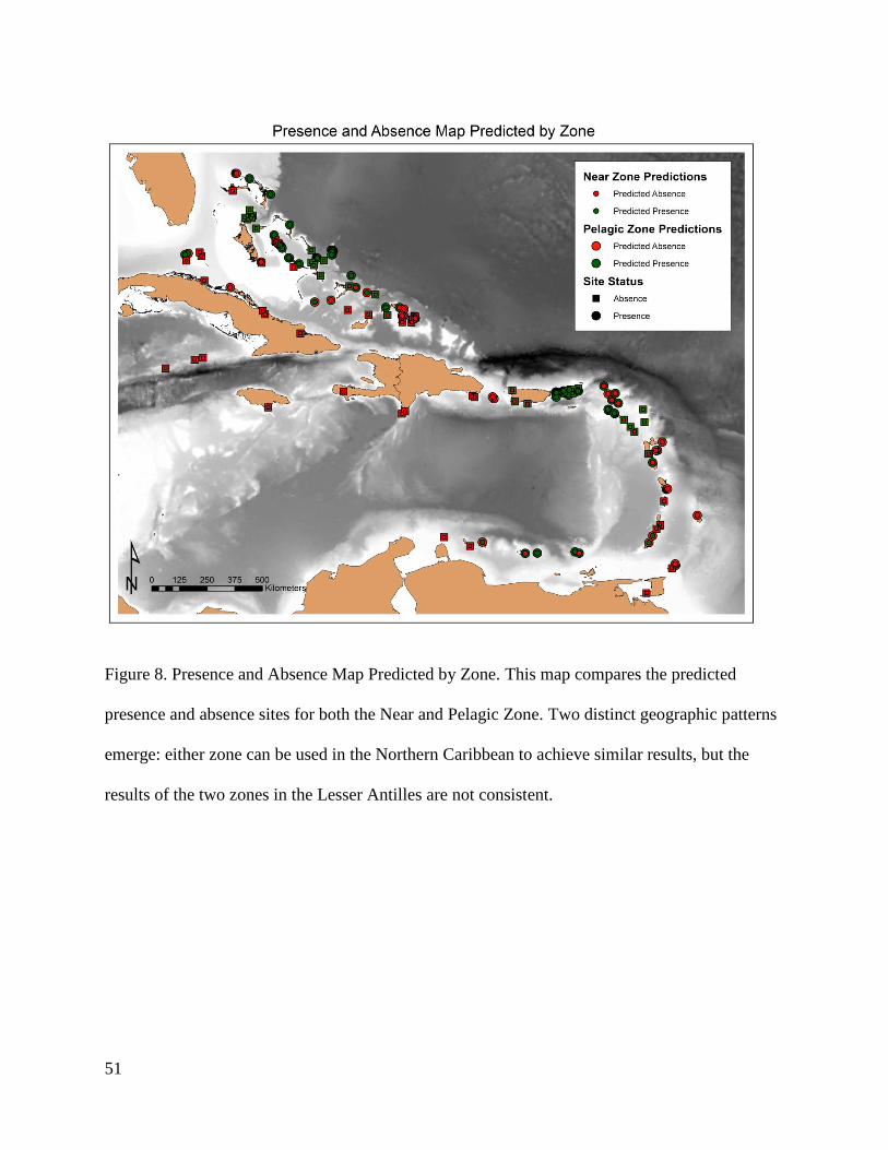
51

Figure 8. Presence and Absence Map Predicted by Zone. This map compares the predicted

presence and absence sites for both the Near and Pelagic Zone. Two distinct geographic patterns

emerge: either zone can be used in the Northern Caribbean to achieve similar results, but the

results of the two zones in the Lesser Antilles are not consistent.

52

Figure 9. Puffinus l. loyemilleri Probability and Prediction Map. This map shows the results of

the P. l. loyemilleri analysis. The map displays the results both by the results of the predicted site

status and the average probability of the two logistic equations.

53

Appendix C: Main Shearwater Shapefile Format

Pre

sen

ce

and

Ab

sen

ceIs

lan

d N

ame

Isla

nd

Gro

up

Maj

or

Ch

ain

Surv

ey

Dat

eJa

nFe

bM

arA

pr

May

Jun

Jul

Au

gSe

pO

ctN

ov

De

cD

EM

Ava

ilab

leLo

ngi

tud

eLa

titu

de

Ne

ar Z

on

e

Pro

bab

ilit

y

Ne

ar

Pre

dic

tio

n

Pe

lagi

c Zo

ne

Pro

bab

ilit

y

Pe

lagi

c

Pre

dic

tio

nD

ata

Sou

rce

0A

bse

nce

1 A

llig

ato

r C

ayEx

um

asG

reat

Bah

ama

Ban

k19

940

01

11

00

00

00

0ye

s-7

6.63

8755

8624

.392

9223

40.

5541

2524

10.

5215

2382

0B

rad

ley

and

No

rto

n 2

009

0A

bse

nce

2 B

oat

Ho

use

Ro

ckR

um

Cay

East

ern

Bah

amas

1989

00

11

10

00

00

00

yes

-74.

8390

1623

.685

4680

10.

6704

8523

10.

7399

8074

1B

rad

ley

and

No

rto

n 2

009

0A

bse

nce

3 B

oo

by

Cay

May

agu

ana

Sou

the

rn B

aham

as19

980

01

11

00

00

00

0ye

s-7

2.71

7844

6622

.326

0434

30.

6982

4584

10.

5605

4599

1B

rad

ley

and

No

rto

n 2

009

0A

bse

nce

4 C

ay S

alC

ay S

alC

ay S

al B

ank

1996

00

11

10

00

00

00

yes

-80.

4114

8974

23.7

0855

721

0.55

8041

351

0.43

5476

630

Bra

dle

y an

d N

ort

on

200

9

0A

bse

nce

5 D

amas

Cay

Cay

Sal

Cay

Sal

Ban

k19

960

01

11

00

00

00

0ye

s-7

9.80

0975

1723

.892

9548

40.

4651

3069

00.

3017

7762

0B

rad

ley

and

No

rto

n 2

009

0A

bse

nce

6 D

ange

r C

ayEx

um

asG

reat

Bah

ama

Ban

k20

060

01

11

00

00

00

0ye

s-7

6.69

7351

8724

.426

3243

40.

5328

5762

10.

4976

166

0B

rad

ley

and

No

rto

n 2

009

0A

bse

nce

7 D

og

Ro

cks

Cay

Sal

Cay

Sal

Ban

k19

960

01

11

00

00

00

0ye

s-7

9.86

2599

624

.048

3661

20.

4743

1598

00.

3216

7207

0B

rad

ley

and

No

rto

n 2

009

0A

bse

nce

8 D

oll

y's

Ro

ckSo

uth

An

dro

sG

reat

Bah

ama

Ban

k19

840

01

11

00

00

00

0ye

s-7

7.67

9852

0223

.745

488

0.32

3000

550

0.38

7907

150

Bra

dle

y an

d N

ort

on

200

9

0A

bse

nce

9 D

uck

Cay

Exu

mas

Gre

at B

aham

a B

ank

1999

00

11

10

00

00

00

yes

-76.

0414

3066

23.4

5117

587

0.49

8338

860

0.49

0738

440

Bra

dle

y an

d N

ort

on

200

9

0A

bse

nce

10

Fro

zen

Cay

Be

rry

Isla

nd

sG

reat

Bah

ama

Ban

k20

020

01

11

00

00

00

0ye

s-7

7.71

8075

0625

.571

9767

40.

6212

4014

10.

6929

6406

1B

rad

ley

and

No

rto

n 2

009

0A

bse

nce

11

Gal

lio

t C

ayLo

ng

Isla

nd

Gre

at B

aham

a B

ank

1991

00

11

10

00

00

00

yes

-75.

3333

3335

23.6

3333

335

0.62

5353

021

0.69

4300

921

Bra

dle

y an

d N

ort

on

200

9

0A

bse

nce

12

Go

ld R

ock

Ack

lin

sSo

uth

ern

Bah

amas

1997

00

11

10

00

00

00

yes

-73.

8865

7794

22.6

7091

095

0.39

5136

990

0.60

6859

71

Bra

dle

y an

d N

ort

on

200

9

0A

bse

nce

13

Go

uld

ing

Cay

Ne

w P

rovi

de

nce

Gre

at B

aham

a B

ank

2003

00

11

10

00

00

00

yes

-77.

5702

4759

25.0

2071

406

0.56

9964

331

0.64

8419

861

Bra

dle

y an

d N

ort

on

200

9

0A

bse

nce

14

Gu

ana

Cay

Cat

Isla

nd

Gre

at B

aham

a B

ank

1986

00

11

10

00

00

00

yes

-75.

3249

7744

24.1

4933

818

0.79

0203

121

0.76

0490

11

Bra

dle

y an

d N

ort

on

200

9

0A

bse

nce

15

Haw

ksb

ill C

ayEx

um

asG

reat

Bah

ama

Ban

k20

000

01

11

00

00

00

0ye

s-7

6.77

1200

824

.496

1551

10.

5153

4748

00.

4719

1345

0B

rad

ley

and

No

rto

n 2

009

0A

bse

nce

16

Ho

gsty

Re

ef

Gre

at In

agu

aSo

uth

ern

Bah

amas

1979

00

11

10

00

00

00

yes

-73.

3238

0465

21.0

6570

430.

5583

8062

10.

4579

449

0B

rad

ley

and

No

rto

n 2

009

0A

bse

nce

17

Litt

le In

agu

aLi

ttle

Inag

ua

Sou

the

rn B

aham

as19

990

01

11

00

00

00

0ye

s-7

3.00

5400

9821

.506

1123

90.

5689

0205

10.

4875

4149

0B

rad

ley

and

No

rto

n 2

009

0A

bse

nce

18

Litt

le P

ige

on

Exu

mas

Gre

at B

aham

a B

ank

1998

00

11

10

00

00

00

yes

-76.

7940

0816

24.5

1262

545

0.52

5550

280

0.46

2937

30

Bra

dle

y an

d N

ort

on

200

9

0A

bse

nce

19

Litt

le W

hal

e C

ayB

err

y Is

lan

ds

Gre

at B

aham

a B

ank

2002

00

11

10

00

00

00

yes

-77.

7599

6685

25.4

4857

939

0.57

4976

111

0.68

1447

241

Bra

dle

y an

d N

ort

on

200

9

0A

bse

nce

20

Mam

ma

Rh

od

a R

ock

Be

rry

Isla

nd

sG

reat

Bah

ama

Ban

k20

020

01

11

00

00

00

0ye

s-7

7.92

1164

6325

.407

6292

30.

5742

4489

10.

6680

3828

1B

rad

ley

and

No

rto

n 2

009

0A

bse

nce

21

Me

rite

k P

on

dLo

ng

Isla

nd

Gre

at B

aham

a B

ank

1990

00

11

10

00

00

00

yes

-75.

0961

5523

.176

424

0.58

9762

851

0.71

3158

751

Bra

dle

y an

d N

ort

on

200

9

0A

bse

nce

22

Pe

ters

on

Cay

Gra

nd

Bah

ama

Litt

le B

aham

a B

ank

2004

00

11

10

00

00

00

no

-78.

5230

8592

26.5

5191

792

0.45

8252

030

0.45

4529

40

Bra

dle

y an

d N

ort

on

200

9

0A

bse

nce

23

Pe

tits

Cay

Be

rry

Isla

nd

sG

reat

Bah

ama

Ban

k20

020

01

11

00

00

00

0ye

s-7

7.83

4125

2725

.771

6163

60.

6310

0413

10.

7256

5215

1B

rad

ley

and

No

rto

n 2

009

0A

bse

nce

24

Ru

m C

ayB

err

y Is

lan

ds

Gre

at B

aham

a B

ank

2002

00

11

10

00

00

00

yes

-77.

8450

6562

25.7

3285

125

0.59

4404

871

0.70

9675

321

Bra

dle

y an

d N

ort

on

200

9

0A

bse

nce

25

Sad

dle

Cay

Exu

mas

Gre

at B

aham

a B

ank

2006

00

11

10

00

00

00

yes

-76.

8085

997

24.6

3590

076

0.50

7145

480

0.45

3943

420

Bra

dle

y an

d N

ort

on

200

9

0A

bse

nce

26

Shro

ud

Cay

Exu

mas

Gre

at B

aham

a B

ank

2005

00

11

10

00

00

00

yes

-76.

7763

9436

24.5

3495

427

0.52

6912

680

0.46

5456

710

Bra

dle

y an

d N

ort

on

200

9

0A

bse

nce

27

Stra

chan

Cay

Lon

g Is

lan

dG

reat

Bah

ama

Ban

k19

900

01

11

00

00

00

0ye

s-7

4.94

5479

7523

.098

1631

90.

5428

687

10.

6744

9157

1B

rad

ley

and

No

rto

n 2

009

0A

bse

nce

28

Big

San

d C

ayTu

rks

Turk

s B

ank

2002

00

11

10

00

00

00

yes

-71.

2481

4124

21.1

9728

940.

4629

0664

00.

3509

398

0B

rad

ley

and

No

rto

n 2

009

0A

bse

nce

29

Bu

sh C

ays

Bu

sh a

nd

Se

als

Cai

cos

Ban

k20

020

01

11

00

00

00

0ye

s-7

1.62

8435

7121

.201

2025

40.

3557

9312

00.

4129

9592

0B

rad

ley

and

No

rto

n 2

009

0A

bse

nce

30

Fish

Cay

Ou

ter

Cai

cos

Cai

cos

Ban

k20

020

01

11

00

00

00

0ye

s-7

1.61

7561

0621

.366

7966

70.

3378

9568

00.

4012

2889

0B

rad

ley

and

No

rto

n 2

009

0A

bse

nce

31

Fre

nch

Isla

nd

Cai

cos

Cai

cos

Ban

k20

020

01

11

00

00

00

0ye

s-7

2.22

6770

721

.493

0376

80.

5272

7009

00.

5628

7134

1B

rad

ley

and

No

rto

n 2

009

0A

bse

nce

32

Gra

nd

Tu

rkTu

rks

Turk

s B

ank

2004

00

11

10

00

00

00

yes

-71.

1389

2904

21.4

6745

869

0.30

0619

260

0.37

8881

680

Bra

dle

y an

d N

ort

on

200

9

0A

bse

nce

33

Lon

g C

ayTu

rks

Turk

s B

ank

2002

00

11

10

00

00

00

yes

-71.

0963

8333

21.4

1352

309

0.28

8616

210

0.35

9105

390

Bra

dle

y an

d N

ort

on

200

9

0A

bse

nce

34

Pe

nn

isto

n C

ayTu

rks

Turk

s B

ank

2002

00

11

10

00

00

00

yes

-71.

1224

4125

21.3

7615

813

0.45

9026

220

0.35

7170

430

Bra

dle

y an

d N

ort

on

200

9

0A

bse

nce

35

Ro

un

d C

ayG

ibb

's C

ayTu

rks

Ban

k20

020

01

11

00

00

00

0ye

s-7

1.11

2544

2221

.441

1204

10.

2938

4718

00.

3679

023

0B

rad

ley

and

No

rto

n 2

009

0A

bse

nce

36

Salt

Cay

Turk

sTu

rks

Ban

k20

040

01

11

00

00

00

0ye

s-7

1.20

7228

1121

.329

2986

10.

2886

0779

00.

3491

9689

0B

rad

ley

and

No

rto

n 2

009

0A

bse

nce

37

Bal

len

ato

Cay

oC

amag

ue

yC

ub

a20

040

00

11

10

00

00

0ye

s-7

7.20

4446

7721

.523

9510

20.

3167

3915

00.

1348

70

Bra

dle

y an

d N

ort

on

200

9

0A

bse

nce

38

Cay

os

Bro

qu

ele

sN

ipe

Bay

Cu

ba

1998

00

01

11

00

00

00

no

-75.

7739

6758

20.7

5162

885

0.31

0281

610

0.12

9829

730

Bra

dle

y an

d N

ort

on

200

9

0A

bse

nce

39

Du

tto

n C

ayo

Los

Paj

on

ale

sC

ub

a20

040

00

11

10

00

00

0ye

s-7

9.67

7752

6722

.891

3492

70.

2420

7924

00.

0833

1495

0B

rad

ley

and

No

rto

n 2

009

0A

bse

nce

40

Sab

inal

Cay

oC

amag

ue

yC

ub

a20

040

00

11

10

00

00

0ye

s-7

7.30

0001

5121

.666

6674

50.

3267

5373

00.

1469

3299

0B

rad

ley

and

No

rto

n 2

009

0A

bse

nce

41

Bo

ob

y P

on

dLi

ttle

Cay

man

Cay

man

Isla

nd

s20

010

02

22

00

00

00

0ye

s-8

0.07

2893

8119

.672

5948

80.

4758

5526

00.

2258

6256

0B

rad

ley

and

No

rto

n 2

009

0A

bse

nce

42

E C

aym

an B

rac

Blu

ffC

aym

an B

rac

Cay

man

Isla

nd

s20

030

02

22

00

00

00

0ye

s-7

9.73

2180

2919

.748

2788

80.

4270

8883

00.

1395

9126

0B

rad

ley

and

No

rto

n 2

009

0A

bse

nce

43

No

rth

So

un

d E

stat

es

Gra

nd

Cay

man

Cay

man

Isla

nd

s19

950

02

22

00

00

00

0ye

s-8

1.26

2337

8719

.320

1038

60.

4448

3933

00.

5143

4523

0B

rad

ley

and

No

rto

n 2

009

0A

bse

nce

44

Litt

le H

alf

Mo

on

Po

rtla

nd

Big

ht

Jam

aica

2005

10

22

20

00

00

00

no

-77.

0869

0573

17.7

3470

858

0.42

2453

930

0.29

3738

740

Bra

dle

y an

d N

ort

on

200

9

0A

bse

nce

45

Isla

Alt

o V

elo

Do

min

ican

Re

pu

bli

cH

isp

anio

la20

050

02

22

00

00

00

0ye

s-7

1.64

0833

8417

.473

0555

90.

4229

8073

00.

3654

8486

0B

rad

ley

and

No

rto

n 2

009

0A

bse

nce

46

Be

ata

Isla

nd

Do

min

ican

Re

pu

bli

cH

isp

anio

la20

050

02

22

00

00

00

0ye

s-7

1.51

3044

17.5

7048

90.

4445

9506

00.

4121

6178

0B

rad

ley

and

No

rto

n 2

009

0A

bse

nce

47

Pas

o d

e C

atu

anSa

on

aH

isp

anio

la20

050

02

22

00

00

00

0 y

es

-68.

7362

6141

18.2

0505

535

0.27

2081

040

0.29

1285

50

Bra

dle

y an

d N

ort

on

200

9

0A

bse

nce

48

Pic

Mac

aya

Mas

sif

de

la H

ott

eH

isp

anio

la19

990

02

22

00

00

00

0ye

s-7

4.01

8686

0918

.370

6108

20.

3614

4613

00.

3469

9855

0B

rad

ley

and

No

rto

n 2

009

0A

bse

nce

49

Sao

na

Do

min

ican

Re

pu

bli

cH

isp

anio

la19

980

02

22

00

00

00

0ye

s-6

8.67

9736

1918

.153

0884

0.28

3560

710

0.30

6601

340

Bra

dle

y an

d N

ort

on

200

9

0A

bse

nce

50

La P

argu

era

Laja

sP

ue

rto

Ric

o20

050

11

11

11

00

00

0ye

s-6

7.04

6610

3117

.974

9857

50.

4597

3774

00.

5715

6842

1B

rad

ley

and

No

rto

n 2

009

0A

bse

nce

51

Mo

rril

lito

Po

nce

Pu

ert

o R

ico

2005

01

11

11

10

00

00

no

-66.

5340

9478

17.8

7989

748

0.43

1139

930

0.60

1766

791

Bra

dle

y an

d N

ort

on

200

9

0A

bse

nce

52

Agu

adil

laA

guad

illa

Pu

ert

o R

ico

2005

01

11

11

10

00

00

yes

-67.

1540

6981

18.4

2744

498

0.42

9373

490

0.56

2005

071

Bra

dle

y an

d N

ort

on

200

9

0A

bse

nce

53

Bo

ob

y R

ock

St. J

oh

nLe

ew

ard

Isla

nd

s19

901

11

11

10

00

00

0n

o-6

4.70

9901

8718

.302

3201

0.71

2826

21

0.71

4648

91

Bra

dle

y an

d N

ort

on

200

9

0A

bse

nce

54

Car

val R

ock

U.S

. Vir

gin

Lee

war

d Is

lan

ds

1999

11

11

11

00

00

00

ye

s-6

4.79

8139

7718

.368

4685

0.69

1647

351

0.68

7268

551

Bra

dle

y an

d N

ort

on

200

9

0A

bse

nce

55

Du

tch

cap

Cay

St. T

ho

mas

Lee

war

d Is

lan

ds

1999

11

11

11

00

00

00

yes

-65.

0618

2085

18.3

7953

252

0.64

6949

331

0.70

4618

591

Bra

dle

y an

d N

ort

on

200

9

0A

bse

nce

56

Kal

kun

Cay

St. T

ho

mas

Lee

war

d Is

lan

ds

1999

11

11

11

00

00

00

no

-65.

0573

8739

18.3

4959

820.

6524

0218

10.

7038

3308

1B

rad

ley

and

No

rto

n 2

009

0A

bse

nce

57

Litt

le H

ans

Loll

ick

Isla

nd

St. T

ho

mas

Lee

war

d Is

lan

ds

1999

11

11

11

00

00

00

yes

-64.

9074

3854

18.4

1023

678

0.67

8386

271

0.67

8007

331

Bra

dle

y an

d N

ort

on

200

9

0A

bse

nce

58

Turt

led

ove

Cay

U.S

. Vir

gin

Lee

war

d Is

lan

ds

1997

11

11

11

00

00

00

yes

-65.

0002

9538

18.3

0864

686

0.67

8158

951

0.70

2846

071

Bra

dle

y an

d N

ort

on

200

9

0A

bse

nce

59

Co

ckro

ach

Vir

gin

Go

rda

Lee

war

d Is

lan

ds

2005

11

00

00

00

00

01

no

-64.

4625

5949

18.4

9600

560.

8179

4298

10.

7755

5009

1B

rad

ley

and

No

rto

n 2

009

0A

bse

nce

60

Gre

en

Cay

Jost

van

Dyk

eLe

ew

ard

Isla

nd

s20

051

10

00

00

00

00

1ye

s-6

4.70

8863

6618

.454

1712

50.

7318

6511

10.

7542

9835

1B

rad

ley

and

No

rto

n 2

009

0A

bse

nce

61

Gra

nd

Isle

tTh

e S

ain

tsLe

ew

ard

Isla

nd

s19

980

02

22

00

00

00

0ye

s-6

1.58

6093

9415

.840

3240

50.

4776

203

00.

6514

6318

1B

rad

ley

and

No

rto

n 2

009

0A

bse

nce

62

Les

Au

gust

ins

Les

Au

gust

ins

Lee

war

d Is

lan

ds

1998

00

22

20

00

00

00

no

-61.

6116

7423

15.8

4418

974

0.48

1818

270

0.65

3475

761

Bra

dle

y an

d N

ort

on

200

9

0A

bse

nce

63

Bo

ob

y Is

lan

dSt

. Kit

tsLe

ew

ard

Isla

nd

s20

040

02

22

00

00

00

0n

o-6

2.61

0202

6417

.226

8258

40.

4854

0171

00.

6129

7533

1B

rad

ley

and

No

rto

n 2

009

0A

bse

nce

64

Mo

nse

rrat

Mo

nts

err

atLe

ew

ard

Isla

nd

s20

050

02

22

00

00

00

0ye

s-6

2.18

7405

9816

.742

5438

50.

5046

1879

00.

6190

7113

1B

rad

ley

and

No

rto

n 2

009

0A

bse

nce

65

Bu

rma

Qu

arry

An

tigu

aLe

ew

ard

Isla

nd

s19

990

02

22

00

00

00

0ye

s-6

1.77

5361

0717

.136

4097

30.

5824

668

10.

6003

8953

1B

rad

ley

and

No

rto

n 2

009

0A

bse

nce

66

Co

dri

ngt

on

Lag

oo

nB

arb

ud

aLe

ew

ard

Isla

nd

s19

990

02

22

00

00

00

0ye

s-6

1.82

5768

5317

.644

5596

90.

5392

7561

10.

6189

2137

1B

rad

ley

and

No

rto

n 2

009

0A

bse

nce

67

Re

do

nd

a Is

lan

dR

ed

on

da

Lee

war

d Is

lan

ds

2004

00

22

20

00

00

00

yes

-62.

3455

1394

16.9

3841

745

0.53

1723

751

0.63

7563

651

Bra

dle

y an

d N

ort

on

200

9

0A

bse

nce

68

St. L

uci

a Is

lan

dSt

. Lu

cia

Lee

war

d Is

lan

ds

2006

00

22

20

00

00

00

yes

-60.

9790

0901

13.9

0970

286

0.50

8023

990

0.49

3712

180

Bra

dle

y an

d N

ort

on

200

9

0A

bse

nce

69

All

-Aw

ash

Isla

nd

Gre

nad

ine

sW

ind

war

d Is

lan

ds

2004

00

22

20

00

00

00

yes

-61.

1432

4599

12.9

1526

165

0.51

4702

470

0.47

4048

920

Bra

dle

y an

d N

ort

on

200

9

0A

bse

nce

70

Bat

tow

iaG

ren

adin

es

Win

dw

ard

Isla

nd

s20

050

02

22

00

00

00

0ye

s-6

1.13

1927

8212

.961

5199

30.

5347

7401

10.

4883

9955

0B

rad

ley

and

No

rto

n 2

009

0A

bse

nce

71

Pe

tit

Can

ou

anG

ren

adin

es

Win

dw

ard

Isla

nd

s20

040

02

22

00

00

00

0ye

s-6

1.28

2665

2712

.789

9158

50.

5565

9386

10.

4484

2661

0B

rad

ley

and

No

rto

n 2

009

0A

bse

nce

72

Smit

h's

Isla

nd

Trin

idad

Sou

th A

me

rica

1998

22

22

00

00

00

00

no

-60.

6526

4425

11.1

8441

746

0.46

5410

870

0.22

6788

680

Bra

dle

y an

d N

ort

on

200

9

0A

bse

nce

73

Sou

thw

est

Co

ast

Trin

idad

Sou

th A

me

rica

1984

22

22

00

00

00

00

yes

-61.

6904

4715

10.1

6993

736

0.09

5189

230

0.06

9621

570

Bra

dle

y an

d N

ort

on

200

9

0A

bse

nce

74

Lago

Re

ef

Aru

ba

Sou

th A

me

rica

2002

22

00

00

00

00

00

yes

-69.

9282

2614

12.4

4731

758

0.43

2457

710

0.11

1705

610

Bra

dle

y an

d N

ort

on

200

9

0A

bse

nce

75

Lago

on

of

Jan

thie

lC

ura

cao

Cu

raca

o20

022

20

00

00

00

00

0ye

s-6

8.86

9032

3612

.085

4682

80.

6366

967

10.

4308

7156

0B

rad

ley

and

No

rto

n 2

009

1A

llan

's C

ayEx

um

asG

reat

Bah

ama

Ban

k20

030

01

11

00

00

00

0ye

s-7

6.84

1288

824

.740

8524

70.

5378

1235

10.

5643

7738

1B

rad

ley

and

No

rto

n 2

009

1A

two

od

Cay

Sam

ana

Cay

Sou

the

rn B

aham

as19

990

01

11

00

00

00

0n

o-7

3.70

1434

4323

.098

5780

20.

7599

6013

10.

6103

629

1B

rad

ley

and

No

rto

n 2

009

1C

atto

Cay

San

Sal

vad

or

East

ern

Bah

amas

2003

00

11

10

00

00

00

no

-74.

4685

7669

24.1

4388

224

0.90

1489

971

0.76

9367

851

Bra

dle

y an

d N

ort

on

200

9

1C

ay V

erd

eR

agge

d Is

lan

ds

Gre

at B

aham

a B

ank

1998

00

11

10

00

00

00

yes

-75.

1848

5676

22.0

2068

209

0.64

9580

291

0.49

3280

570

Bra

dle

y an

d N

ort

on

200

9

1C

han

ne

l Cay

Exu

mas

Gre

at B

aham

a B

ank

2002

00

11

10

00

00

00

yes

-75.

8012

9354

23.5

5691

323

0.54

5545

361

0.57

8304

871

Bra

dle

y an

d N

ort

on

200

9

54

Pre

sen

ce

and

Ab

sen

ceIs

lan

d N

ame

Isla

nd

Gro

up

Maj

or

Ch

ain

Surv

ey

Dat

eJa

nFe

bM

arA

pr

May

Jun

Jul

Au

gSe

pO

ctN

ov

De

cD

EM

Ava

ilab

leLo

ngi

tud

eLa

titu

de

Ne

ar Z

on

e

Pro

bab

ilit

y

Ne

ar

Pre

dic

tio

n

Pe

lagi

c Zo

ne

Pro

bab

ilit

y

Pe

lagi

c

Pre

dic

tio

nD

ata

Sou

rce

1C

on

cep

tio

n Is

lan

dC

on

cep

tio

nEa

ste

rn B

aham

as19

980

01

11

00

00

00

0ye

s-7

5.11

3672

1223

.834

5389

50.

6789

784

10.

7487

7395

1B

rad

ley

and

No

rto

n 2

009

1C

ut

Cay

San

Sal

vad

or

East

ern

Bah

amas

2003

00

11

10

00

00

00

yes

-74.

4592

0936

24.1

2846

231

0.90

4728

581

0.77

3292

861

Bra

dle

y an

d N

ort

on

200

9

1D

ou

ble

-he

ade

d S

ho

ts C

ayC

ay S

alC

ay S

al B

ank

1984

00

11

10

00

00

00

yes

-80.

3292

7579

23.9

9931

858

0.56

4511

971

0.53

8114

490

Bra

dle

y an

d N

ort

on

200

9

1Ea

st P

imb

lico

Cay

Exu

mas

Gre

at B

aham

a B

ank

2002

00

11

10

00

00

00

yes

-76.

2170

2985

23.8

0683

946

0.55

4772

411

0.59

7426

881

Bra

dle

y an

d N

ort

on

200

9

1Ea

st P

lan

a C

ayP

lan

a C

ays

Sou

the

rn B

aham

as19

980

01

11

00

00

00

0ye

s-7

3.50

8501

2822

.606

5019

0.45

8604

110

0.57

5686

41

Bra

dle

y an

d N

ort

on

200

9

1El

bo

w C

ayC

ay S

alC

ay S

al B

ank

2005

00

11

10

00

00

00

yes

-80.

4612

004

23.9

5086

894

0.58

8800

331

0.57

3667

481

Bra

dle

y an

d N

ort

on

200

9

1El

eu

the

ra Is

lan

dEl

eu

the

raG

reat

Bah

ama

Ban

k19

990

01

11

00

00

00

0ye

s-7

6.66

4493

9225

.467

7565

20.

7867

2554

10.

7356

5113

1B

rad

ley

and

No

rto

n 2

009

1Fi

sh C

ayA

bac

oLi

ttle

Bah

ama

Ban

k19

980

01

11

00

00

00

0ye

s-7

7.83

6892

5927

.048

6324

10.

5703

1996

10.

6966

1529

1B

rad

ley

and

No

rto

n 2

009

1G

auli

n C

aySa

n S

alva

do

rEa

ste

rn B

aham

as20

030

01

11

00

00

00

0n

o-7

4.47

3220

6124

.138

2496

10.

9020

5034

10.

7699

2598

1B

rad

ley

and

No

rto

n 2

009

1G

ou

ldin

g C

aySa

n S

alva

do

rEa

ste

rn B

aham

as20

030

01

11

00

00

00

0n

o-7

4.42

8515

8724

.078

8282

50.

8998

4021

10.

7689

0724

1B

rad

ley

and

No

rto

n 2

009

1G

rah

am's

Har

bo

ur

San

Sal

vad

or

East

ern

Bah

amas

2003

00

11

10

00

00

00

yes

-74.

4646

7022

24.1

1842

599

0.90

5675

971

0.77

4324

431

Bra

dle

y an

d N

ort

on

200

9

1G

ree

n C

aySa

n S

alva

do

rEa

ste

rn B

aham

as20

030

01

11

00

00

00

0ye

s-7

4.50

7627

1424

.138

8947

90.

8022

0407

10.

5955

9261

1B

rad

ley

and

No

rto

n 2

009

1H

igh

Cay

San

Sal

vad

or

East

ern

Bah

amas

2003

00

11

10

00

00

00

yes

-74.

4761

704

23.9

4773

272

0.89

9237

371

0.75

2578

441

Bra

dle

y an

d N

ort

on

200

9

1Li

ttle

Cis

tern

Cay

Exu

mas

Gre

at B

aham

a B

ank

2006

00

11

10

00

00

00

yes

-76.

7425

9965

24.4

5623

794

0.52

3755

90

0.47

7789

270

Bra

dle

y an

d N

ort

on

200

9

1Li

ttle

Wal

ker'

s C

ayW

alke

r's

Cay

Litt

le B

aham

a B

ank

1999

00

11

10

00

00

00

yes

-78.

4031

1138

27.2

5921

063

0.47

6202

480

0.51

5730

010

Bra

dle

y an

d N

ort

on

200

9

1Lo

ng

Cay

Exu

mas

Gre

at B

aham

a B

ank

2000

00

11

10

00

00

00

yes

-76.

1153

2404

23.6

9446

806

0.55

0517

561

0.51

4986

620

Bra

dle

y an

d N

ort

on

200

9

1Lo

w C

aySa

n S

alva

do

rEa

ste

rn B

aham

as20

030

01

11

00

00

00

0ye

s-7

4.48

2216

5323

.936

4031

70.

8985

9675

10.

7520

2626

1B

rad

ley

and

No

rto

n 2

009

1M

alab

ars

Cay

Exu

mas

Gre

at B

aham

a B

ank

2006

00

11

10

00

00

00

yes

-76.

6327

7599

24.3

6674

638

0.55

8314

581

0.52

5076

410

Bra

dle

y an

d N

ort

on

200

9

1M

an H

ead

Cay

San

Sal

vad

or

East

ern

Bah

amas

2003

00

11

10

00

00

00

no

-74.

4503

6063

24.1

2300

032

0.90

5661

991

0.77

1924

771

Bra

dle

y an

d N

ort

on

200

9

1M

ayag

uan

a Is

lan

dM

ayag

uan

aSo

uth

ern

Bah

amas

2005

00

11

10

00

00

00

yes

-73.

0641

4672

22.4

0177

941

0.70

5836

931

0.55

9049

690

Bra

dle

y an

d N

ort

on

200

9

1N

ancy

Cay

San

Sal

vad

or

East

ern

Bah

amas

2000

00

11

10

00

00

00

yes

-74.

4762

2235

23.9

6266

579

0.89

6590

341

0.75

3345

021

Bra

dle

y an

d N

ort

on

200

9

1N

od

dy

Cay

Exu

mas

Gre

at B

aham

a B

ank

2000

00

11

10

00

00

00

no

-76.

1326

1635

23.6

9548

413

0.54

8159

811

0.51

8523

140

Bra

dle

y an

d N

ort

on

200

9

1N

ort

h P

oin

t B

luff

Cay

San

Sal

vad

or

East

ern

Bah

amas

2000

00

11

10

00

00

00

yes

-74.

4588

5608

24.1

2456

310.

9053

9653

10.

7741

3014

1B

rad

ley

and

No

rto

n 2

009

1P

eli

can

Cay

Ab

aco

Litt

le B

aham

a B

ank

2004

00

11

10

00

00

00

yes

-76.

9797

5793

26.4

0303

427

0.75

5749

091

0.87

7360

311

Bra

dle

y an

d N

ort

on

200

9

1P

ige

on

Cre

ek

San

Sal

vad

or

East

ern

Bah

amas

2003

00

11

10

00

00

00

yes

-74.

4842

8124

23.9

7658

496

0.89

5043

841

0.75

7077

1B

rad

ley

and

No

rto

n 2

009

1R

ock

y D

un

das

Exu

mas

Gre

at B

aham

a B

ank

1994

00

11

10

00

00

00

yes

-76.

5405

6214

24.2

7497

196

0.58

8552

891

0.57

2708

721

Bra

dle

y an

d N

ort

on

200

9

1Sa

n S

alva

do

r Is

lan

dSa

n S

alva

do

rEa

ste

rn B

aham

as19

990

01

11

00

00

00

0ye

s-7

4.47

6019

4124

.077

5564

70.

9007

8893

10.

7696

5049

1B

rad

ley

and

No

rto

n 2

009

1Sa

nd

y C

ayEx

um

asG

reat

Bah

ama

Ban

k20

050

01

11

00

00

00

0ye

s-7

5.43

3952

8123

.403

8115

40.

6065

3901

10.

6040

2565

1B

rad

ley

and

No

rto

n 2

009

1So

uth

Mir

a-P

or

Vo

s Is

lan

dM

ira-

po

r-vo

sSo

uth

ern

Bah

amas

1987

00

11

10

00

00

00

yes

-74.

5251

8163

22.0

9168

721

0.51

5709

650

0.53

7801

970

Bra

dle

y an

d N

ort

on

200

9

1So

uth

Ro

cks

Cay

Co

nce

pti

on

East

ern

Bah

amas

1998

00

11

10

00

00

00

yes

-75.

0832

7253

23.8

0901

527

0.65

5576

441

0.74

7223

81

Bra

dle

y an

d N

ort

on

200

9

1Th

e G

ulf

Blu

ffs

San

Sal

vad

or

East

ern

Bah

amas

2000

00

11

10

00

00

00

yes

-74.

5005

319

23.9

4795

359

0.89

2906

521

0.74

7973

771

Bra

dle

y an

d N

ort

on

200

9

1To

m B

row

n's

Cay

Wal

ker'

s C

ayLi

ttle

Bah

ama

Ban

k19

840

01

11

00

00

00

0ye

s-7

8.41

1129

227

.266

2120

50.

4743

0737

00.

5127

1053

0B

rad

ley

and

No

rto

n 2

009

1Tw

ins

Cay

Exu

mas

Gre

at B

aham

a B

ank

1994

00

11

10

00

00

00

yes

-76.

5067

5824

24.2

0954

730.

5933

5081

10.

5918

7236

1B

rad

ley

and

No

rto

n 2

009

1W

ash

erw

om

an C

aySo

uth

An

dro

sG

reat

Bah

ama

Ban

k19

840

01

11

00

00

00

0ye

s-7

7.36

5229

8223

.646

9375

50.

3409

9923

00.

4202

5391

0B

rad

ley

and

No

rto

n 2

009

1W

est

Pim

bli

co C

ayEx

um

asG

reat

Bah

ama

Ban

k20

020

01

11

00

00

00

0ye

s-7

6.24

5273

23.8

2085

087

0.56

8899

741

0.60

5936

631

Bra

dle

y an

d N

ort

on

200

9

1Ea

st C

ayTu

rks

Turk

s B

ank

2005

00

11

10

00

00

00

yes

-71.

0876

6117

21.3

5626

438

0.45

9833

340

0.34

7651

350

Bra

dle

y an

d N

ort

on

200

9

1Fi

ve C

ays

Pro

vid

en

cial

es

Cai

cos

Ban

k20

040

01

11

00

00

00

0ye

s-7

2.25

3475

9521

.735

7148

50.

6718

1002

10.

6464

0206

1B

rad

ley

and

No

rto

n 2

009

1Lo

ng

Cay

1C

aico

sC

aico

s B

ank

2005

00

11

10

00

00

00

yes

-71.

5593

2949

21.4

6496

913

0.37

2004

210

0.42

0986

840

Bra

dle

y an

d N

ort

on

200

9

1M

idd

le C

aico

s Is

lan

dM

idd

le C

aico

sC

aico

s B

ank

2005

00

11

10

00

00

00

yes

-71.

7385

0402

21.7

9451

798

0.52

9894

980

0.63

4518

571

Bra

dle

y an

d N

ort

on

200

9

1N

ort

he

rn C

oas

tEa

st C

aico

sC

aico

s B

ank

2004

00

11

10

00

00

00

yes

-71.

5486

4698

21.7

3053

634

0.34

5030

120

0.51

4870

840

Bra

dle

y an

d N

ort

on

200

9

1Si

xHil

ls C

aySo

uth

Cai

cos

Cai

cos

Ban

k20

040

01

11

00

00

00

0ye

s-7

1.62

8714

2621

.460

9293

0.40

1391

610

0.43

0092

20

Bra

dle

y an

d N

ort

on

200

9

1C

ayo

Fe

lip

e e

l Ch

ico

Cie

go d

e A

vila

Cu

ba

2000

00

01

10

00

00

00

yes

-78.

6234

3676

22.6

1126

809

0.07

8568

160

0.06

0220

840

Bra

dle

y an

d N

ort

on

200

9

1A

lcar

raza

Cu

leb

raP

ue

rto

Ric

o20

050

11

11

11

00

00

0n

o-6

5.36

9151

8618

.361

2937

0.55

4957

711

0.60

9513

061

Bra

dle

y an

d N

ort

on

200

9

1C

ayo

de

l Agu

aC

ule

bra

Pu

ert

o R

ico

2005

01

11

11

10

00

00

no

-65.

3475

1716

18.3

1155

404

0.57

2848

071

0.61

3964

371

Bra

dle

y an

d N

ort

on

200

9

1G

en

iqu

iC

ule

bra

Pu

ert

o R

ico

2005

01

11

11

10

00

00

yes

-65.

2303

426

18.3

3800

848

0.61

2857

91

0.64

7924

921

Bra

dle

y an

d N

ort

on

200

9

1Lo

bit

o C

ayC

ule

bra

Pu

ert

o R

ico

2005

01

11

11

10

00

00

yes

-65.

3917

9172

18.3

3404

40.

5499

2129

10.

6030

488

1B

rad

ley

and

No

rto

n 2

009

1M

ato

jo C

ayC

ule

bra

Pu

ert

o R

ico

2005

01

11

11

10

00

00

yes

-65.

2893

6162

18.3

3661

020.

5992

3805

10.

6322

9838

1B

rad

ley

and

No

rto

n 2

009

1M

on

a Is

lan

dM

ayag

ue

zP

ue

rto

Ric

o20

050

11

11

11

00

00

0ye

s-6

7.89

2742

8818

.082

9054

0.38

0680

70

0.44

3048

190

Bra

dle

y an

d N

ort

on

200

9

1M

on

ito

Isla

nd

May

agu

ez

Pu

ert

o R

ico

2005

01

11

11

10

00

00

yes

-67.

9527

2452

18.1

5534

987

0.37

9225

470

0.44

2918

470

Bra

dle

y an

d N

ort

on

200

9

1R

ato

nC

ule

bra

Pu

ert

o R

ico

2005

01

11

11

10

00

00

no

-65.

3529

545

18.3

1408

612

0.57

0522

871

0.61

3868

711

Bra

dle

y an

d N

ort

on

200

9

1Ye

rba

Cay

Cu

leb

raP

ue

rto

Ric

o20

050

11

11

11

00

00

0n

o-6

5.35

3682

9418

.318

9022

60.

6008

9089

10.

6056

8102

1B

rad

ley

and

No

rto

n 2

009

1C

ock

roac

h Is

lan

dSt

. Th

om

asLe

ew

ard

Isla

nd

s19

991

11

11

10

00

00

0ye

s-6

5.05

9803

18.4

0400

186

0.64

1224

511

0.70

1736

891

Bra

dle

y an

d N

ort

on

200

9

1Fl

at C

ayU

.S. V

irgi

nLe

ew

ard

Isla

nd

s19

991

11

11

10

00

00

0n

o-6

4.98

9878

1318

.316

7879

80.

6804

2398

10.

6994

1629

1B

rad

ley

and

No

rto

n 2

009

1Fr

en

chca

pSt

. Th

om

asLe

ew

ard

Isla

nd

s19

991

11

11

10

00

00

0ye

s-6

4.85

1141

118

.232

0194

20.

7453

6092

10.

7170

1942

1B

rad

ley

and

No

rto

n 2

009

1Sa

ba

Cay

St. T

ho

mas

Lee

war

d Is

lan

ds

1999

11

11

11

00

00

00

yes

-64.

9999

4513

18.3

0547

486

0.67

8841

031

0.70

2232

771

Bra

dle

y an

d N

ort

on

200

9

1Su

la C

aySt

. Th

om

asLe

ew

ard

Isla

nd

s20

051

11

11

10

00

00

0ye

s-6

5.05

7082

0218

.402

9550

80.

6413

0047

10.

7026

3328

1B

rad

ley

and

No

rto

n 2

009

1B

roke

n J

eru

sale

mG

inge

rLe

ew

ard

Isla

nd

s20

051

10

00

00

00

00

1ye

s-6

4.45

7426

4418

.404

8112

30.

8218

4837

10.

7893

0934

1B

rad

ley

and

No

rto

n 2

009

1C

oo

pe

rIsl

and

Co

op

er

Lee

war

d Is

lan

ds

2005

11

00

00

00

00

01

yes

-64.

5072

9837

18.3

8084

467

0.83

9867

181

0.78

9424

311

Bra

dle

y an

d N

ort

on

200

9

1G

inge

rIsl

and

Gin

ger

Lee

war

d Is

lan

ds

2005

11

00

00

00

00

01

yes

-64.

4754

0989

18.3

9013

610.

8282

4697

10.

7893

9413

1B

rad

ley

and

No

rto

n 2

009

1G

reat

To

bag

oJo

st v

an D

yke

Lee

war

d Is

lan

ds

2005

11

00

00

00

00

01

yes

-64.

8244

2398

18.4

4540

30.

7301

7686

10.

7412

9549

1B

rad

ley

and

No

rto

n 2

009

1D

og

Isla

nd

An

guil

laLe

ew

ard

Isla

nd

s20

050

11

11

10

00

00

0ye

s-6

3.25

3527

9718

.280

8041

40.

4327

3322

00.

5580

0884

0B

rad

ley

and

No

rto

n 2

009

1So

mb

rero

Isla

nd

An

guil

laLe

ew

ard

Isla

nd

s20

050

11

11

10

00

00

0ye

s-6

3.42

3756

8918

.600

1615

50.

4173

8014

00.

6019

9126

1B

rad

ley

and

No

rto

n 2

009

1P

eli

can

Ke

ySt

. Maa

rtin

Lee

war

d Is

lan

ds

2004

00

11

10

00

00

00

yes

-63.

0963

641

18.0

2989

895

0.45

7840

870

0.57

2468

311

Bra

dle

y an

d N

ort

on

200

9

1O

ld B

oo

by

Hil

lSa

ba

Lee

war

d Is

lan

ds

2004

11

11

10

00

00

00

yes

-63.

2180

2762

17.6

3453

294

0.54

9078

431

0.74

8919

21

Bra

dle

y an

d N

ort

on

200

9

1Fo

rt B

aySa

ba

Lee

war

d Is

lan

ds

2004

11

11

10

00

00

00

yes

-63.

2442

5825

17.6

1521

272

0.54

5505

971

0.74

2640

771

Bra

dle

y an

d N

ort

on

200

9

1G

reat

Po

int

Sab

aLe

ew

ard

Isla

nd

s20

021

11

11

00

00

00

0ye

s-6

3.24

2791

2517

.647

7914

60.

5467

4866

10.

7456

0484

1B

rad

ley

and

No

rto

n 2

009

1Su

lph

ur

Min

eSa

ba

Lee

war

d Is

lan

ds

2004

11

11

10

00

00

00

yes

-63.

2312

8438

17.6

4470

804

0.54

8883

951

0.74

7478

421

Bra

dle

y an

d N

ort

on

200

9

1W

ell

's B

aySa

ba

Lee

war

d Is

lan

ds

2004

11

11

10

00

00

00

yes

-63.

2513

4949

17.6

4089

519

0.54

5348

711

0.74

2347

311

Bra

dle

y an

d N

ort

on

200

9

1G

allo

w's

Bay

St. E

ust

atiu

sLe

ew

ard

Isla

nd

s20

031

11

11

00

00

00

0ye

s-6

2.98

4411

0617

.476

8885

10.

5272

2262

00.

7219

4608

1B

rad

ley

and

No

rto

n 2

009

1Tu

mb

le D

ow

n D

ick

Bay

St. E

ust

atiu

sLe

ew

ard

Isla

nd

s19

981

11

11

00

00

00

0ye

s-6

2.99

7336

5917

.500

4610

30.

5311

4804

10.

7286

5042

1B

rad

ley

and

No

rto

n 2

009

1D

esi

rad

e Is

lan

dD

esi

rad

eLe

ew

ard

Isla

nd

s20

020

02

22

22

00

00

0ye

s-6

1.05

0047

16.3

2086

0.46

1445

940

0.49

5987

480

Bra

dle

y an

d N

ort

on

200

9

1N

E Fa

lais

es

Mar

ie G

alan

teLe

ew

ard

Isla

nd

s20

020

01

11

11

00

00

0ye

s-6

1.23

8363

3715

.982

4391

10.

4774

8803

00.

4347

1452

0B

rad

ley

and

No

rto

n 2

009

1St

. Bar

tsSt

. Bar

tho

lom

ew

Lee

war

d Is

lan

ds

2002

00

22

20

00

00

00

yes

-62.

8333

3317

.90.

4607

8745

00.

5689

6517

1B

rad

ley

and

No

rto

n 2

009

1V

ieu

x Fo

rtM

arie

Gal

ante

Lee

war

d Is

lan

ds

2002

00

11

10

00

00

00

yes

-61.

3038

3053

15.9

7769

328

0.42

9379

350

0.51

8107

670

Bra

dle

y an

d N

ort

on

200

9

1B

urg

aux

Mar

tin

iqu

eLe

ew

ard

Isla

nd

s20

040

01

11

00

00

00

0n

o-6

0.83

9071

814

.409

0503

90.

5024

0334

00.

5048

9867

0B

rad

ley

and

No

rto

n 2

009

1D

esi

rad

eM

arti

niq

ue

Lee

war

d Is

lan

ds

2005

00

11

10

00

00

00

yes

-60.

8739

4765

14.3

8850

216

0.49

5247

750

0.49

3183

870

Bra

dle

y an

d N

ort

on

200

9

1P

erc

eM

arti

niq

ue

Lee

war

d Is

lan

ds

2004

00

11

10

00

00

00

no

-60.

8378

6703

14.4

1432

421

0.49

1277

620

0.50

6300

950

Bra

dle

y an

d N

ort

on

200

9

1B

ird

Ro

ckB

arb

ado

sW

ind

war

d Is

lan

ds

2005

11

11

11

11

11

11

yes

-59.

6192

9915

13.3

3077

013

0.48

4192

920

0.45

8813

270

Bra

dle

y an

d N

ort

on

200

9

1C

arri

aco

u C

om

ple

xG

ren

ada

Win

dw

ard

Isla

nd

s20

020

01

11

00

00

00

0ye

s-6

1.44

2875

7112

.503

5791

40.

5777

2026

10.

3542

3159

0B

rad

ley

and

No

rto

n 2

009

1G

ree

n C

ayG

ren

ada

Win

dw

ard

Isla

nd

s19

540

01

11

00

00

00

0ye

s-6

1.58

9292

1912

.221

5050

50.

6750

8556

10.

5484

9191

0B

rad

ley

and

No

rto

n 2

009

55

Pre

sen

ce

and

Ab

sen

ceIs

lan

d N

ame

Isla

nd

Gro

up

Maj

or

Ch

ain

Surv

ey

Dat

eJa

nFe

bM

arA

pr

May

Jun

Jul

Au

gSe

pO

ctN

ov

De

cD

EM

Ava

ilab

leLo

ngi

tud

eLa

titu

de

Ne

ar Z

on

e

Pro

bab

ilit

y

Ne

ar

Pre

dic

tio

n

Pe

lagi

c Zo

ne

Pro

bab

ilit

y

Pe

lagi

c

Pre

dic

tio

nD

ata

Sou

rce

1Li

ttle

Tob

ago

Tob

ago

Sou

th A

me

rica

2004

11

11

00

00

00

00

yes

-60.

5022

8175

11.2

9813

454

0.49

7105

840

0.28

4137

130

Bra

dle

y an

d N

ort

on

200

9

1St

. Gil

es

Tob

ago

Sou

th A

me

rica

2004

11

11

00

00

00

00

yes

-60.

5216

0509

11.3

5611

847

0.50

1607

490

0.29

9113

870

Bra

dle

y an

d N

ort

on

200

9

1B

on

aire

Bo

nai

reB

on

aire

2014

11

00

00

00

00

00

yes

-68.

2385

3412

.178

361

0.56

2839

051

0.43

2306

270

De

lne

vo 2

014

1El

Bla

nq

uil

la Is

lan

dV

en

ezu

ela

Ce

ntr

al C

arib

be

an19

941

10

00

00

00

00

0ye

s-6

4.59

3564

9411

.847

7875

50.

5565

7232

10.

6636

9053

1B

rad

ley

and

No

rto

n 2

009

1La

Orc

hil

a Is

lan

dV

en

ezu

ela

Ce

ntr

al C

arib

be

an20

051

10

00

00

00

00

0ye

s-6

6.12

9629

11.7

9492

50.

5432

3862

10.

7681

0997

1B

rad

ley

and

No

rto

n 2

009

1Is

la lo

s H

erm

ano

sV

en

ezu

ela

Ce

ntr

al C

arib

be

an20

051

00

00

00

00

00

0ye

s-6

4.42

2961

6911

.794

3562

10.

5178

5909

00.

6041

8623

1B

rad

ley

and

No

rto

n 2

009

1Lo

s R

oq

ue

s Is

lan

dLo

s R

oq

ue

sC

en

tral

Car

ibb

ean

2005

11

00

00

00

00

00

yes

-66.

6197

3401

11.7

8615

282

0.44

2925

890

0.69

1961

541

Bra

dle

y an

d N

ort

on

200

9

1Li

ttle

Scr

ub

Isla

nd

An

guil

laLe

ew

ard

Isla

nd

s20

110

02

22

10

00

00

0ye

s-6

2.95

6337

8218

.302

6673

50.

4669

675

00.

5605

0747

1H

od

ge 2

011

1M

ou

nt

Dia

bo

ltin

Do

min

ica

Lee

war

d Is

lan

ds

00

01

11

00

00

00

0ye

s-6

1.44

0622

915

.486

2747

60.

5119

7424

00.

5671

7904

1Le

vesq

ue

an

d Y

eso

u 2

005

56

Appendix D: Puffinus l. loyemilleri Shapefile

Ra

nk

Na

me

Isla

nd

Gro

up

Ma

in G

rou

pLa

st

Surv

ey

Jan

Feb

Ma

rA

pr

Ne

ar

Zon

e

Pro

ba

bil

itie

s

Pe

lagi

c Zo

ne

Pro

ba

bil

itie

s

Ne

ar

Pre

dic

tio

n

Pe

lagi

c

Pre

dic

tio

n

Me

an

Pro

ba

bil

ity

Lon

gitu

de

Lati

tud

e

1La

s To

rtu

guil

las

La T

ort

uga

Ve

ne

zue

laU

nkn

ow

n1

10

00

.61

68

31

85

50

.67

79

66

98

21

10

.64

73

99

42

-65

.43

28

64

10

.96

06

43

2B

ub

ies

Ba

joLa

Ro

qu

es

Ve

ne

zue

laU

nkn

ow

n1

10

00

.44

31

74

10

00

.65

53

56

12

10

10

.54

92

65

11

-66

.59

20

58

11

.82

71

24

3K

lein

Cu

raca

oC

ura

cao

Cu

raca

o2

00

21

10

00

.55

72

06

83

80

.10

60

42

38

81

00

.33

16

24

61

-68

.64

50

57

11

.99

01

96

4Is

lote

Su

cre

San

An

dre

sC

olu

mb

iaU

nkn

ow

n1

10

00

.45

33

08

39

50

.53

74

00

73

60

00

.49

53

54

57

-81

.69

05

71

12

.60

35

26

5R

ich

mo

nd

Isla

nd

Tob

ago

Tob

ago

Un

kno

wn

11

11

0.4

65

83

00

37

0.2

19

63

11

94

00

0.3

42

73

06

2-6

0.5

95

52

61

1.2

18

51

1

6P

ue

rto

Re

al

Los

Fra

ile

s Is

.V

en

ezu

ela

19

45

11

00

0.4

11

08

83

43

0.1

32

68

89

37

00

0.2

71

88

86

4-6

3.7

36

35

41

1.2

01

26

9

7Is

la la

So

laLo

s Fr

ail

es

Is.

Ve

ne

zue

laU

nkn

ow

n1

10

00

.39

07

84

06

30

.14

40

42

43

30

00

.26

74

13

25

-63

.56

97

08

11

.31

37

22

8Is

la d

e P

ato

sV

en

ezu

ela

Ve

ne

zue

laU

nkn

ow

n1

11

10

.24

93

69

09

00

.10

62

04

10

80

00

.17

77

86

60

-61

.86

85

56

10

.63

51

48

9M

on

jes

de

l Su

rLo

s M

on

jes

Co

lum

bia

Un

kno

wn

11

00

0.2

80

66

51

22

0.0

18

48

99

11

00

0.1

49

57

75

2-7

0.9

05

57

71

2.3

46

44

1

An Assessment of Factors Affecting the Spatial ...

Documents

Transcript of An Assessment of Factors Affecting the Spatial ...