An Assessment of CFD Cavitation Models UsingBubble Growth Theory and Bubble TransportModelingMichael P. Kinzel1*, Robert F. Kunz2, Jules W. Lindau 1

SYM

POSI

A

ON ROTATING MACHIN

ERY

ISROMAC 2017

InternationalSymposium on

Transport Phenomenaand

Dynamics of RotatingMachinery

Maui, Hawaii

December 16-21, 2017

AbstractThis effort investigates two approaches to cavitation modeling that are relevant to computa-tional fluid dynamics (CFD). The two approaches include (1) reformulating the cavitationmodels and (2) exploring the impact of liquid-vapor slip. The first aspect of the paperrevisits cavitation model formulations with respect to the Rayleigh-Plesset Equation (RPE).The approach reformulates the cavitation model using analytic solutions to the RPE. Thebenefit of this reformulation is displayed through maintaining model sensitivities similarto RPE, whereas the standard models fail these tests. In addition, the model approach isextended beyond standard homogenous models to a two-fluid model framework that includesbubble slip. The results indicate a significant impact of slip on the predicted cavitationsolution, suggesting that inclusion of such modeling can potentially improve CFD cavitationmodels. Overall, the results of this effort point to various aspects that should be consideredin future CFD-modeling efforts that aim to model cavitation.KeywordsCFD – Cavitation Modeling – Approximate Bubble Dynamics – Bubble Transport1Applied Research Laboratory, Department of Aerospace Engineering, The Pennsylvania State University2Department of Mechanical Engineering, The Pennsylvania State University*Corresponding author: mpk176@alumni.psu.edu

INTRODUCTIONCavitation relates to marine applications, pump designs,rockets, and a variety of other liquid flows. In gen-eral, this is an undesired physical process that is highlynon-linear and strongly impacts performance. For thesereasons, modeling cavitation using computational fluiddynamics (CFD) has become important for the design ofcomplex systems. Because of this, maturing physicallyaccurate models for cavitation remains useful.

In the context of CFD, there are various approachesto cavitation modeling. A common approach is basedon a volume of fluids (VOF)-like approach, coupled witha model for the exchange from a liquid to vapor phase(evaporation) and vice versa (condensation). These mod-els are commonly referred to as homogenous multiphasemodels [1, 2, 3, 4]. These approaches have all improvedsignificantly in their reliability over the years, but stillpose challenges in complexity, mesh requirements, anddifficult-to-ascertain empirical factors. Such a modelaims to directly conserve and transport vapor mass anduses source terms to model the evaporation and conden-sation processes. A vapor-mass conservation equationused is given by [1, 2]:

∂(ρvαv)∂t

+ ∂(ρvαvui)∂xi

= mevap − mcond (1)

Here, ρv is the vapor density, αv is the vapor volume frac-

tion, and the source terms, mevap and mcond, model evap-oration and condensation rates, respectively. Addition-ally, ui and xi are the Cartesian velocity and directionalcomponents. When combined with a Navier-Stokes-basedsolver, via fluid properties, such an approach enables themodeling of cavitation.

Cavitation modeling aims to approximate the sourceterms in the vapor conservation equation, i.e., mevap −mcond, and is an area that continues to progress. Theinitial efforts of Merkle [1] and Kunz [2] were more fo-cused on numerics and developed heuristic models forcavitation. Later, the Rayleigh-Plesset Equation (RPE)was explored as a physics-based method to improve cavi-tation models. The RPE is a model that predicts nucleigrowth, collapse, and the dynamics associated with it[5, 6]. The resulting nonliner, second-order ordinarydifferential equation is given as:

RR+ 32 R

2 + 4νlRR

+ 2SρlR

= pv − pρl

+ pG0

ρl

(R0

R

)3γ)(2)

This model describes the dynamics of an isolated bubblewith a radius R as it is exposed to a driving pressure, p.Some of the other quantities in this relation are the liquidfluid properties, i.e., kinematic viscosity (νl), density (ρl),and saturated vapor pressure (pv). In addition, the nucleiproperties such as its initial radius, R0, and pressure,pG0 , as well as the surface tension, S. This RPE is a

Cavitation Model Assessment — 2/11

physics-based model that gives accurate predictions ofcavitation behavior.

In the context of Eulerian-based cavitation models,reduced forms of the RPE were explored in the efforts ofSinghal et al. [4], Sauer and Schnerr [3], and Zwart et al.[7]. These models all aim to model evaporation and con-densation processes using a reduced RPE. One issue withthese models is that modeling evaporation and condensa-tion processes are processes completely neglected in theRPE. Such a modeling discrepancy still remains withinthe Eulerian CFD models for cavitation. Alternatively,Lagrangian modeling efforts of the cavitation process alsoexist [8, 9] and do so without the aforementioned model-ing mismatch. These Lagrangian efforts directly modelthe cavitation processes using RPE and do in fact predictnuclei growth and collapse. Despite their progress andimproved physical accuracy, these Lagrangian modelsremain as an isolated branch of cavitation modeling fromthe Eulerian efforts. Some efforts seem to be movingto better include such cavitation dynamics as indicatedby Wang and Brennen [10] for quasi-one-dimensionalflows and Balu [11, 12] for flows without advection. Inaddition, recent work [13] evaluated traditional cavita-tion model formulations with respect to the RPE. Inthe evaluations, it was found that the present model-ing approaches are all first-order representations of thecavitation and neglect several terms that lead to inaccu-racy. In this work, we focus on exploring CFD cavitationmodels with respect to cavitation dynamics as describedusing by the RPE. The present efforts essentially pushthe understanding of CFD-based cavitation modeling tobetter incorporate bubble dynamics (from a growth andtransport perspectives).

A second aspect of the paper intends to focus on thetransport of the cavitation bubbles. Specifically, the ac-curacy of the homogenous model assumption is evaluated.This intends to address the issue of whether or not thevelocity vector in Eqn. (1) should be the same for thebubble and liquid phases. This fundamental question,common to boiling flows, that to the authors’ knowledgeis yet to be addressed in the context of cavitation. Com-bining and utilizing these two approaches, we believe weare working to develop an improved cavitation model.The present paper is outlined as follows. The numericalmethods and test cases used for the final assessmentsare presented. This is followed by a reformulation of thecavitation model and assessments of its accuracy withrespect to the RPE for simple isolated bubble scenarios.Next, we present a two-fluid modeling approach for acavitating flow with bubble slip with respect to the liquid.This is followed by a comparison of the various modelformulations to evaluate the overall sensitivity of theeffect of cavitation modeling and bubble slip. Lastly, thefindings from these efforts are summarized with respectto future cavitation modeling.

1. NUMERICAL METHODS

The present study is developed in the context of thecommercial CFD code, Star-CCM+ [14]. In this work,we use a two-fluid, Eulerian-based multiphase-modelingapproach that aims to conserve phase mass througha volume-of-fluid-like formulation. The CFD modelis based on a pressure-based, segregated-flow modelthat conserves mass and momentum of two differentphases. For the liquid water phase, an incompressiblemodel is used where the liquid properties are as fol-lows: ρl = 1000kg/m3, µl = 0.001Pa− s. The gas phaseassumes an incompressible gas model with properties sim-ilar to air, i.e., ρv = 1.2kg/m3, µv = 1.85× 10−5Pa− s.Note that air properties are used as they are both similarto vapor and, as discussed through this work, cavitationinvolves mixtures of nuclei and vapor gas. Hence, thefluid properties relevant to cavitation models is not purevapor and this assumption should not affect the accu-racy of the model. Throughout this work, each phaseconsists of its own velocity vector. Note that the ho-mogenous model is achieved using drag values that drivethe slip to very low values. The numerical scheme isformally second-order accurate in space (upwind, finitevolume) and time (backward difference). In terms of theturbulence, a Reynolds Averaged Navier-Stokes (RANS)turbulence model is used. The model is based on theSpalart-Allmaras turbulence model [15]. Note that thepresent analyses are independent of turbulence modeland findings should extend to any turbulence modelchoice.

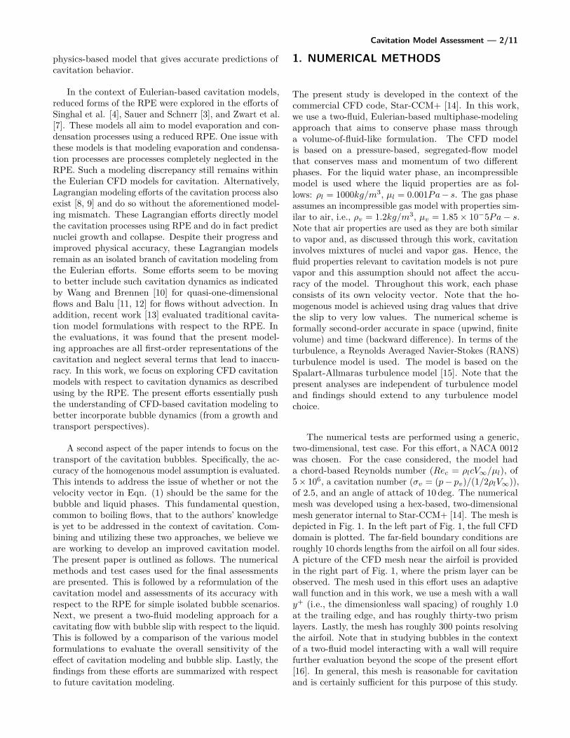
The numerical tests are performed using a generic,two-dimensional, test case. For this effort, a NACA 0012was chosen. For the case considered, the model hada chord-based Reynolds number (Rec = ρlcV∞/µl), of5× 106, a cavitation number (σv = (p− pv)/(1/2ρlV∞)),of 2.5, and an angle of attack of 10 deg. The numericalmesh was developed using a hex-based, two-dimensionalmesh generator internal to Star-CCM+ [14]. The mesh isdepicted in Fig. 1. In the left part of Fig. 1, the full CFDdomain is plotted. The far-field boundary conditions areroughly 10 chords lengths from the airfoil on all four sides.A picture of the CFD mesh near the airfoil is providedin the right part of Fig. 1, where the prism layer can beobserved. The mesh used in this effort uses an adaptivewall function and in this work, we use a mesh with a wally+ (i.e., the dimensionless wall spacing) of roughly 1.0at the trailing edge, and has roughly thirty-two prismlayers. Lastly, the mesh has roughly 300 points resolvingthe airfoil. Note that in studying bubbles in the contextof a two-fluid model interacting with a wall will requirefurther evaluation beyond the scope of the present effort[16]. In general, this mesh is reasonable for cavitationand is certainly sufficient for this purpose of this study.

Cavitation Model Assessment — 3/11

Figure 1. Computational mesh used in the CFD studies throughout this effort. The left figure plots the full CFDdomain and the right figure plots a blowup near the hydrofoil.

2. REFORMULATED CAVITATION MODEL2.1 Cavitation Model FormulationThe first aspect of the present effort aims to improvecavitation modeling by more faithfully representing theRPE. In the context of a VOF-like formulation, the vapormass conservation equation can be written as [1, 2]:

∂(ρv,effαv)∂t

+∂(ρv,effαvui)∂xi

= ρv,eff (SV,evap−SV,cond)

(3)

Note the source terms are now referred to as ρv,eff (SV,evap−SV,cond), where SV,evap and SV,cond respectively repre-sent the volume growth and shrinkage of nuclei. Thisform is preferred as the RPE is a volume change modeland does not model phase change. The effective vapordensity, ρv,eff , is introduced as an effective density ofthe vapor for which the momentum is based upon. Ingeneral, the true density cannot be used as cavitation isboth compressible and composed of multiple gas species.To investigate improving cavitation models, we use aprocess that transforms from R to αv. Note that R isthe radius of an isolated bubble and is the dependent pa-rameter in the RPE. With the use of a physically-basedinput, i.e., bubble concentration, Nb, there is a directrelation between volume fraction and bubble radius [13],which is given as

αv = Nb43πR

3. (4)

Note that Nb is described as the number of bubbles perunit volume. Similarly, the rate-of-change in volumefraction can be described (for an incompressible model)as

αv = Nb43π

d

dt(R3) = 4πNbR2R. (5)

Similarly, the second-rate-of-change in volume fractioncan be described as

αv = Nb4πd

dt(R2R) = 4πNb(R2R+ 2RR2). (6)

Such transformations enable cavitation models to bedirectly based on the RPE. Although there are manychoices to incorporate RPE into CFD-based cavitationmodels [3, 4, 7, 8], what the present effort aims to findare the key terms associated with the RPE with respectto CFD cavitation models. In the work of Kinzel et al[13], analytic solutions of bubble dynamics from Brennen[17] are used as reference solutions. In the present work,the application of those analytic solutions is extendedto provide an alternative basis for the formulation ofa cavitation model. Here, the radial growth rate of abubble is estimated using an analytic solution to the RPEwith the assumption of a step change in the pressure,yielding[17]:

R =(

23

(pv − p)ρl

[1− R3

0R3

]

+ 23pg0

ρl

11− γ

[R3γ

0R3γ −

R30

R3

](7)

+ 2SρlR

[1− R2

0R2

])1/2

Note that in this model form, the viscosity term was ne-glected to arrive at this analytic solution[17]. In addition,in outside of nucleation and collapse events, R0 << 1,surface tension is of lower importance, hence, the relationreduces to

R =(

23

(pv − p)ρl

+ 23pg0

ρl

11− γ

[R3γ

0R3γ −

R30

R3

])1/2

. (8)

This analytic solution provides a RPE-based model thatcan help construct a physically-based cavitation modelfor bubble growth. In terms of the driving terms (inthe root), present cavitation models are limited to thefirst term, i.e., (pv − p)/ρl, and the remaining terms areneglected. When the model is converted into a source

Cavitation Model Assessment — 4/11

term, the following model is obtained

SV,evap =CevapC∞

× α2/3v

(23

(pv − p)ρl

+ 23pg0

ρl

11− γ

[αγ0αγ− αv,0

α

])1/2

, (9)

where the nucleation-site concentration is assumed to beconstant and yields its associated constant as

C∞ =N

1/3b

62/3 π1/3. (10)

Note that this is a model that is distinctly different thanprevious works [1, 2, 3, 4, 7].

Now consider the bubble collapse events. These mod-els are then, similarly, modeled using a model for bubblecollapse [17] given as

R =−(RmaxR

)3/2(23

(p− pv)ρl

+ 23pg0

ρl

11− γ

R3γ0

R3γ −2SρlR

)1/2

(11)

Neglecting surface tension, this approach reduces to

R = −(RmaxR

)3/2(23

(p− pv)ρl

+ 23pg0

ρl

11− γ

R3γ0

R3γ

)1/2

(12)

Then converting to CFD-variables, a model for the bubblegrowth can be obtained as

SV,cond = CcondC∞α2/3v

(αmaxα

)1/2

×

(23

(p− pv)ρl

+ 23pg0

ρl

11− γ

αγv,0αγ

)1/2

, (13)

One last issue is the αv,max term, which is a time-history-related quantity that is not an algebraically computedvalue at a given point in the flow field. The challengeof this term arises as there is a time history associatedwith it and obtaining such a quantity is not well suitedto CFD models without an auxiliary transport equation.For the current state of the model, it is assumed thatαv,max = 1.0, which implies that the collapse energy isbased on the maximum bubble size available. Hence,the model is expected to be accurate when processedthrough a sheet cavity. However, in cloud cavitation,where volume fractions do not reach unity in CFD, themodel will likely over-estimate the collapse rate in cloud

cavitation. With this assumption, the model simplifiesto

SV,evap = CcondC∞α1/6v

×

(23

(p− pv)ρl

+ 23pg0

ρl

11− γ

αγv,0αγ

)1/2

. (14)

The resulting model provides a CFD model that rep-resents the RPE in the same way as the approximatemodels do for the bubble dynamics. Prior to proceed-ing, it is important to list the underlying assumptionsof this modeling approach. To the best of the authors’knowledge, these assumptions are as follows:

1. The underlying assumptions of the RPE are re-tained (i.e., spherical bubbles, no interaction withneighboring bubbles, no thermal cavitation)

2. Cavitation process relevant to CFD behave likegroups of bubbles governed by RPE

3. The model breaks down as the vapor volume frac-tion approaches unity (i.e., sheet cavities), andthe concept of subgrid-scale isolated bubbles it nolonger valid

4. Constant nuclei distribution through the fluid do-main

5. Cavitation collapse goes through a process of thelargest nuclei growth possible.

Keeping these assumptions in mind, one goal of thiseffort is to develop a more physically accurate cavitationmodel.

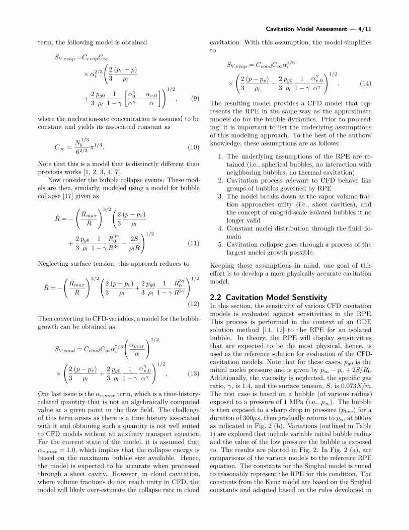
2.2 Cavitation Model SenstivityIn this section, the sensitivity of various CFD cavitationmodels is evaluated against sensitivities in the RPE.This process is performed in the context of an ODEsolution method [11, 12] to the RPE for an isolatedbubble. In theory, the RPE will display sensitivitiesthat are expected to be the most physical, hence, isused as the reference solution for evaluation of the CFD-cavitation models. Note that for these cases, pg0 is theinitial nuclei pressure and is given by p∞ − pv + 2S/R0.Additionally, the viscosity is neglected, the specific gasratio, γ, is 1.4, and the surface tension, S, is 0.073N/m.The test case is based on a bubble (of various radius)exposed to a pressure of 1 MPa (i.e., p∞). The bubbleis then exposed to a sharp drop in pressure (plow) for aduration of 300µs, then gradually returns to p∞ at 500µsas indicated in Fig. 2 (b). Variations (outlined in Table1) are explored that include variable initial bubble radiusand the value of the low pressure the bubble is exposedto. The results are plotted in Fig. 2. In Fig. 2 (a), arecomparisons of the various models to the reference RPEequation. The constants for the Singhal model is tunedto reasonably represent the RPE for this condition. Theconstants from the Kunz model are based on the Singhalconstants and adapted based on the rules developed in

Cavitation Model Assessment — 5/11

Kinzel et al. [13]. The overall results indicate that, whenthe cavitation constants are correctly established, theSinghal and Kunz models replicate the RPE. Note thatthis is also expected to occur for the Sauer, Zwart andMerkle models. The result of Fig. 2 (a) is equivalentto establishing CFD-cavitation model constants for asingle condition, and a test of the fidelity of the model isunderstanding how well the model extrapolates to otherconditions.

(a) Case 1: R0 = 20µm, plow = 0.1pv

(b) General pressure profile

Figure 2. Comparison of the predictions from the RPE,Singhal, Kunz, and Reformulated models for the growthand collapse of an isolated bubble exposed to pressurein part (b). This plot indicates that the cavitationmodels can replicate the RPE.

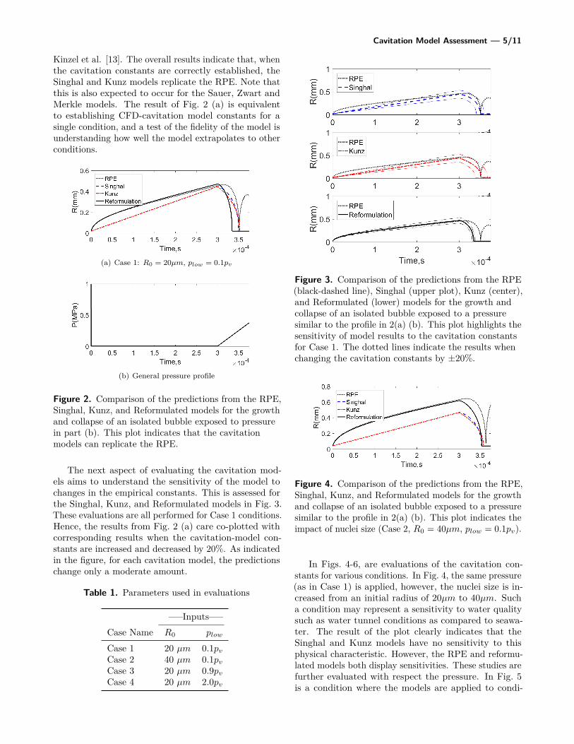
The next aspect of evaluating the cavitation mod-els aims to understand the sensitivity of the model tochanges in the empirical constants. This is assessed forthe Singhal, Kunz, and Reformulated models in Fig. 3.These evaluations are all performed for Case 1 conditions.Hence, the results from Fig. 2 (a) care co-plotted withcorresponding results when the cavitation-model con-stants are increased and decreased by 20%. As indicatedin the figure, for each cavitation model, the predictionschange only a moderate amount.

Table 1. Parameters used in evaluations

—–Inputs—–Case Name R0 plow

Case 1 20 µm 0.1pvCase 2 40 µm 0.1pvCase 3 20 µm 0.9pvCase 4 20 µm 2.0pv

Figure 3. Comparison of the predictions from the RPE(black-dashed line), Singhal (upper plot), Kunz (center),and Reformulated (lower) models for the growth andcollapse of an isolated bubble exposed to a pressuresimilar to the profile in 2(a) (b). This plot highlights thesensitivity of model results to the cavitation constantsfor Case 1. The dotted lines indicate the results whenchanging the cavitation constants by ±20%.

Figure 4. Comparison of the predictions from the RPE,Singhal, Kunz, and Reformulated models for the growthand collapse of an isolated bubble exposed to a pressuresimilar to the profile in 2(a) (b). This plot indicates theimpact of nuclei size (Case 2, R0 = 40µm, plow = 0.1pv).

In Figs. 4-6, are evaluations of the cavitation con-stants for various conditions. In Fig. 4, the same pressure(as in Case 1) is applied, however, the nuclei size is in-creased from an initial radius of 20µm to 40µm. Sucha condition may represent a sensitivity to water qualitysuch as water tunnel conditions as compared to seawa-ter. The result of the plot clearly indicates that theSinghal and Kunz models have no sensitivity to thisphysical characteristic. However, the RPE and reformu-lated models both display sensitivities. These studies arefurther evaluated with respect the pressure. In Fig. 5is a condition where the models are applied to condi-

Cavitation Model Assessment — 6/11

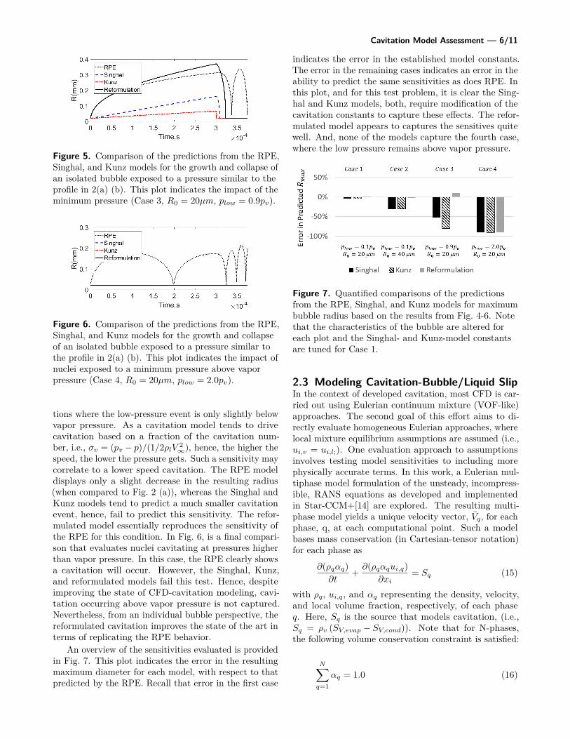
Figure 5. Comparison of the predictions from the RPE,Singhal, and Kunz models for the growth and collapse ofan isolated bubble exposed to a pressure similar to theprofile in 2(a) (b). This plot indicates the impact of theminimum pressure (Case 3, R0 = 20µm, plow = 0.9pv).

Figure 6. Comparison of the predictions from the RPE,Singhal, and Kunz models for the growth and collapseof an isolated bubble exposed to a pressure similar tothe profile in 2(a) (b). This plot indicates the impact ofnuclei exposed to a minimum pressure above vaporpressure (Case 4, R0 = 20µm, plow = 2.0pv).

tions where the low-pressure event is only slightly belowvapor pressure. As a cavitation model tends to drivecavitation based on a fraction of the cavitation num-ber, i.e., σv = (pv − p)/(1/2ρlV 2

∞), hence, the higher thespeed, the lower the pressure gets. Such a sensitivity maycorrelate to a lower speed cavitation. The RPE modeldisplays only a slight decrease in the resulting radius(when compared to Fig. 2 (a)), whereas the Singhal andKunz models tend to predict a much smaller cavitationevent, hence, fail to predict this sensitivity. The refor-mulated model essentially reproduces the sensitivity ofthe RPE for this condition. In Fig. 6, is a final compari-son that evaluates nuclei cavitating at pressures higherthan vapor pressure. In this case, the RPE clearly showsa cavitation will occur. However, the Singhal, Kunz,and reformulated models fail this test. Hence, despiteimproving the state of CFD-cavitation modeling, cavi-tation occurring above vapor pressure is not captured.Nevertheless, from an individual bubble perspective, thereformulated cavitation improves the state of the art interms of replicating the RPE behavior.

An overview of the sensitivities evaluated is providedin Fig. 7. This plot indicates the error in the resultingmaximum diameter for each model, with respect to thatpredicted by the RPE. Recall that error in the first case

indicates the error in the established model constants.The error in the remaining cases indicates an error in theability to predict the same sensitivities as does RPE. Inthis plot, and for this test problem, it is clear the Sing-hal and Kunz models, both, require modification of thecavitation constants to capture these effects. The refor-mulated model appears to captures the sensitives quitewell. And, none of the models capture the fourth case,where the low pressure remains above vapor pressure.

Figure 7. Quantified comparisons of the predictionsfrom the RPE, Singhal, and Kunz models for maximumbubble radius based on the results from Fig. 4-6. Notethat the characteristics of the bubble are altered foreach plot and the Singhal- and Kunz-model constantsare tuned for Case 1.

2.3 Modeling Cavitation-Bubble/Liquid SlipIn the context of developed cavitation, most CFD is car-ried out using Eulerian continuum mixture (VOF-like)approaches. The second goal of this effort aims to di-rectly evaluate homogeneous Eulerian approaches, wherelocal mixture equilibrium assumptions are assumed (i.e.,ui,v = ui,l;). One evaluation approach to assumptionsinvolves testing model sensitivities to including morephysically accurate terms. In this work, a Eulerian mul-tiphase model formulation of the unsteady, incompress-ible, RANS equations as developed and implementedin Star-CCM+[14] are explored. The resulting multi-phase model yields a unique velocity vector, Vq, for eachphase, q, at each computational point. Such a modelbases mass conservation (in Cartesian-tensor notation)for each phase as

∂(ρqαq)∂t

+ ∂(ρqαqui,q)∂xi

= Sq (15)

with ρq, ui,q, and αq representing the density, velocity,and local volume fraction, respectively, of each phaseq. Here, Sq is the source that models cavitation, (i.e.,Sq = ρv (SV,evap − SV,cond)). Note that for N-phases,the following volume conservation constraint is satisfied:

N∑q=1

αq = 1.0 (16)

Cavitation Model Assessment — 7/11

Momentum conservation for each phase (both gas andliquid) is expressed as

∂(ρqαquj,q)∂t

+ ∂(ρqαqui,quj,q)∂xi

=− αq∂p

∂xj

+ ∂τi,j,q∂xj

(17)

+ FHyd,j,q,p

In this relation, FHyd,j,q,p is the hydrodynamic-basedmomentum exchange occurring on phase q through hy-drodynamic forces with the other phase, p. A realistictwo-fluid model that captures slip demands a reasonablemodel of the drag behavior.

Formulation of the drag force typically requires a dragmodel that is based on a normalized drag coefficient. Thehydrodynamic force for such a model can be describedas

FHyd,j,q,p = Kj,q,p[uj,q − uj,p] (18)

The model for the momentum exchange coefficient, Kj,q,p,is defined according to the content of vapor bubbles. Themodel form is described as

Kj,q,p = 0.75αqαpµldv

Req,pcD, (19)

where the drag coefficient is given by the modified Schiller-Naumann [18] model given as

cD = kB24

Req,p(1.0 + 0.15Re0.687

q,p ). (20)

Here, Req,p is the Reynolds number based on the carrier-fluid properties, slip velocity, and the size of the bubble,and is defined as

Req,p = ρldvVslipµl

, (21)

where Vslip = |Vv − VL|. Also, kB is a modificationconstant that is applied to account for bubbles. Lastly,the bubble diameter is the last unclosed parameter, whichis estimated using spherical assumptions and is given as

dv = 2 3

√3

4παvNB

(22)

Such a model is fully closed and provides a platformto evaluate the impact of the homogenous model forcavitation prediction.

Before moving forward, it is worth a discussion of thetwo-fluid model drag model with respect to cavitation.In general, the larger value of cD, and lighter the fluidenables drives the model to conditions that are homoge-nous. In this work, and for consistency, a homogenousmodel is obtained by setting the bubble diameter to1µm, essentially providing a large cD value that forcesvelocity equilibrium. With respect to the model that

aims to capture slip, a model for the bubble drag isconstructed. Presently available bubble drag models arenot clearly applicable to cavitation [19, 20]. Specifically,the main dependency, gravity, is not directly applicableto cavitation. Hence, the current model modified theSchiller-Naumann model using a value of kB of 16/24,which is based on the efforts of Kay and Nedderman [21]of the drag behavior in the Stokes regime. This modelis reasonable for this initial analysis but certainly, needsadvancement moving forward.

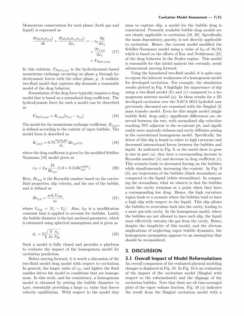
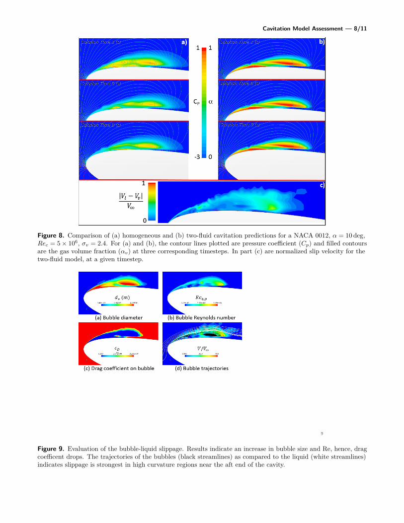
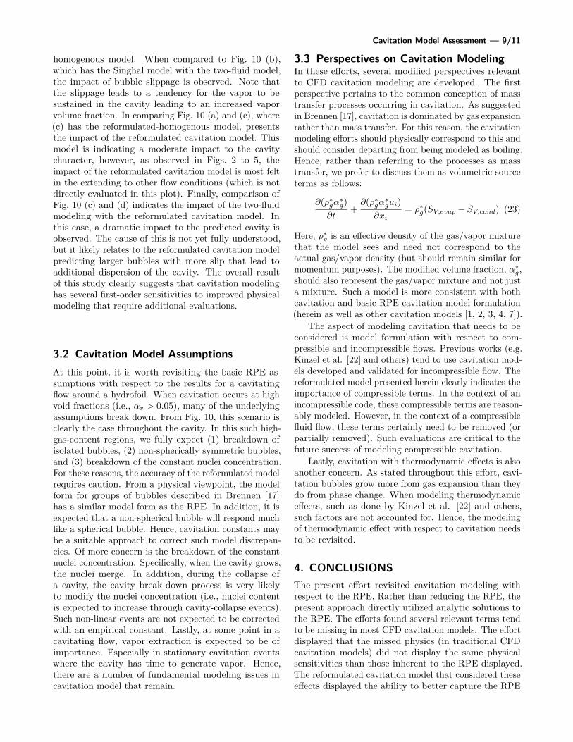
Using the formulated two-fluid model, it is quite easyto expose the inherent weaknesses of a homogenous modelfor developed cavitation. For example, the simulationresults plotted in Fig. 8 highlight the importance of slipusing a two-fluid model (b) and (c) compared to a ho-mogenous mixture model (a). In these results for a 2Ddeveloped cavitation over the NACA 0012 hydrofoil casepreviously discussed are examined with the Singhal [4]mass transfer model. Even for this simple model (singlebubble field, drag only), significant differences are ob-served between the two, with normalized slip velocitiesreaching 70% adjacent to the re-entrant jet, and signifi-cantly more unsteady richness and cavity diffusion arisingin the conventional homogenous model. Specifically, thedriver of this slip is found to relate to high curvature anddecreased interactional forces between the bubbles andliquid. As indicated in Fig. 9, as the nuclei show to growin size in part (a), they have a corresponding increase inReynolds number (b) and decrease in drag coefficient (c).This scenario leads to decreased forcing on the bubbles,while simultaneously increasing the content. In Fig. 9(d), are trajectories of the bubbles (black streamlines) ascompared to the liquid (white streamlines). In compar-ing the streamlines, what we observe is that the bubblesreach the cavity terminus at a point when they havea corresponding low drag. Hence, the high curvatureregion leads to a scenario where the bubbles tend to havea high slip with respect to the liquid. This slip allowsthe bubbles to recirculate back into the cavity, leading toa more gas-rich cavity. In the homogenous model, wherethe bubbles are not allowed to have such slip, the liquidmore effectively entrains the gas from the cavity. Hence,despite the simplicity of this model, and the obviousimplications of neglecting vapor bubble dynamics, thehomogenous assumption appears to an assumption thatshould be reconsidered.

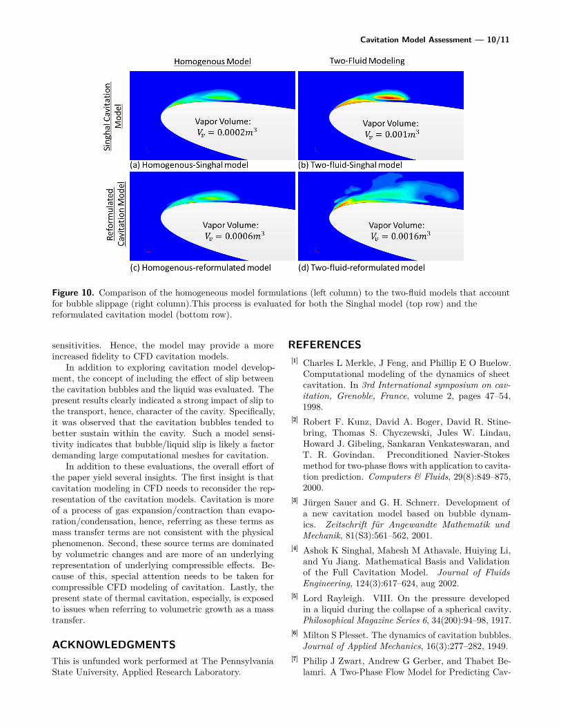
3. DISCUSSION3.1 Overall Impact of Model ReformulationsAn overall comparison of the evaluated physical modelingchanges is displayed in Fig. 10. In Fig. 10 is an evaluationof the impact of the cavitation model (Singhal withrespect to the reformulated) and the slippage of thecavitation bubbles. Note that these are all time-averagedplots of the vapor volume fraction. Fig. 10 (a) indicatesthe result from the Singhal cavitation model with a

Cavitation Model Assessment — 8/11

Figure 8. Comparison of (a) homogeneous and (b) two-fluid cavitation predictions for a NACA 0012, α = 10 deg,Rec = 5× 106, σv = 2.4. For (a) and (b), the contour lines plotted are pressure coefficient (Cp) and filled contoursare the gas volume fraction (αv) at three corresponding timesteps. In part (c) are normalized slip velocity for thetwo-fluid model, at a given timestep.

Figure 9. Evaluation of the bubble-liquid slippage. Results indicate an increase in bubble size and Re, hence, dragcoefficent drops. The trajectories of the bubbles (black streamlines) as compared to the liquid (white streamlines)indicates slippage is strongest in high curvature regions near the aft end of the cavity.

Cavitation Model Assessment — 9/11

homogenous model. When compared to Fig. 10 (b),which has the Singhal model with the two-fluid model,the impact of bubble slippage is observed. Note thatthe slippage leads to a tendency for the vapor to besustained in the cavity leading to an increased vaporvolume fraction. In comparing Fig. 10 (a) and (c), where(c) has the reformulated-homogenous model, presentsthe impact of the reformulated cavitation model. Thismodel is indicating a moderate impact to the cavitycharacter, however, as observed in Figs. 2 to 5, theimpact of the reformulated cavitation model is most feltin the extending to other flow conditions (which is notdirectly evaluated in this plot). Finally, comparison ofFig. 10 (c) and (d) indicates the impact of the two-fluidmodeling with the reformulated cavitation model. Inthis case, a dramatic impact to the predicted cavity isobserved. The cause of this is not yet fully understood,but it likely relates to the reformulated cavitation modelpredicting larger bubbles with more slip that lead toadditional dispersion of the cavity. The overall resultof this study clearly suggests that cavitation modelinghas several first-order sensitivities to improved physicalmodeling that require additional evaluations.

3.2 Cavitation Model AssumptionsAt this point, it is worth revisiting the basic RPE as-sumptions with respect to the results for a cavitatingflow around a hydrofoil. When cavitation occurs at highvoid fractions (i.e., αv > 0.05), many of the underlyingassumptions break down. From Fig. 10, this scenario isclearly the case throughout the cavity. In this such high-gas-content regions, we fully expect (1) breakdown ofisolated bubbles, (2) non-spherically symmetric bubbles,and (3) breakdown of the constant nuclei concentration.For these reasons, the accuracy of the reformulated modelrequires caution. From a physical viewpoint, the modelform for groups of bubbles described in Brennen [17]has a similar model form as the RPE. In addition, it isexpected that a non-spherical bubble will respond muchlike a spherical bubble. Hence, cavitation constants maybe a suitable approach to correct such model discrepan-cies. Of more concern is the breakdown of the constantnuclei concentration. Specifically, when the cavity grows,the nuclei merge. In addition, during the collapse ofa cavity, the cavity break-down process is very likelyto modify the nuclei concentration (i.e., nuclei contentis expected to increase through cavity-collapse events).Such non-linear events are not expected to be correctedwith an empirical constant. Lastly, at some point in acavitating flow, vapor extraction is expected to be ofimportance. Especially in stationary cavitation eventswhere the cavity has time to generate vapor. Hence,there are a number of fundamental modeling issues incavitation model that remain.

3.3 Perspectives on Cavitation ModelingIn these efforts, several modified perspectives relevantto CFD cavitation modeling are developed. The firstperspective pertains to the common conception of masstransfer processes occurring in cavitation. As suggestedin Brennen [17], cavitation is dominated by gas expansionrather than mass transfer. For this reason, the cavitationmodeling efforts should physically correspond to this andshould consider departing from being modeled as boiling.Hence, rather than referring to the processes as masstransfer, we prefer to discuss them as volumetric sourceterms as follows:

∂(ρ∗gα∗g)∂t

+∂(ρ∗gα∗gui)

∂xi= ρ∗g(SV,evap − SV,cond) (23)

Here, ρ∗g is an effective density of the gas/vapor mixturethat the model sees and need not correspond to theactual gas/vapor density (but should remain similar formomentum purposes). The modified volume fraction, α∗g,should also represent the gas/vapor mixture and not justa mixture. Such a model is more consistent with bothcavitation and basic RPE cavitation model formulation(herein as well as other cavitation models [1, 2, 3, 4, 7]).

The aspect of modeling cavitation that needs to beconsidered is model formulation with respect to com-pressible and incompressible flows. Previous works (e.g.Kinzel et al. [22] and others) tend to use cavitation mod-els developed and validated for incompressible flow. Thereformulated model presented herein clearly indicates theimportance of compressible terms. In the context of anincompressible code, these compressible terms are reason-ably modeled. However, in the context of a compressiblefluid flow, these terms certainly need to be removed (orpartially removed). Such evaluations are critical to thefuture success of modeling compressible cavitation.

Lastly, cavitation with thermodynamic effects is alsoanother concern. As stated throughout this effort, cavi-tation bubbles grow more from gas expansion than theydo from phase change. When modeling thermodynamiceffects, such as done by Kinzel et al. [22] and others,such factors are not accounted for. Hence, the modelingof thermodynamic effect with respect to cavitation needsto be revisited.

4. CONCLUSIONSThe present effort revisited cavitation modeling withrespect to the RPE. Rather than reducing the RPE, thepresent approach directly utilized analytic solutions tothe RPE. The efforts found several relevant terms tendto be missing in most CFD cavitation models. The effortdisplayed that the missed physics (in traditional CFDcavitation models) did not display the same physicalsensitivities than those inherent to the RPE displayed.The reformulated cavitation model that considered theseeffects displayed the ability to better capture the RPE

Cavitation Model Assessment — 10/11

Figure 10. Comparison of the homogeneous model formulations (left column) to the two-fluid models that accountfor bubble slippage (right column).This process is evaluated for both the Singhal model (top row) and thereformulated cavitation model (bottom row).

sensitivities. Hence, the model may provide a moreincreased fidelity to CFD cavitation models.

In addition to exploring cavitation model develop-ment, the concept of including the effect of slip betweenthe cavitation bubbles and the liquid was evaluated. Thepresent results clearly indicated a strong impact of slip tothe transport, hence, character of the cavity. Specifically,it was observed that the cavitation bubbles tended tobetter sustain within the cavity. Such a model sensi-tivity indicates that bubble/liquid slip is likely a factordemanding large computational meshes for cavitation.

In addition to these evaluations, the overall effort ofthe paper yield several insights. The first insight is thatcavitation modeling in CFD needs to reconsider the rep-resentation of the cavitation models. Cavitation is moreof a process of gas expansion/contraction than evapo-ration/condensation, hence, referring as these terms asmass transfer terms are not consistent with the physicalphenomenon. Second, these source terms are dominatedby volumetric changes and are more of an underlyingrepresentation of underlying compressible effects. Be-cause of this, special attention needs to be taken forcompressible CFD modeling of cavitation. Lastly, thepresent state of thermal cavitation, especially, is exposedto issues when referring to volumetric growth as a masstransfer.

ACKNOWLEDGMENTSThis is unfunded work performed at The PennsylvaniaState University, Applied Research Laboratory.

REFERENCES[1] Charles L Merkle, J Feng, and Phillip E O Buelow.

Computational modeling of the dynamics of sheetcavitation. In 3rd International symposium on cav-itation, Grenoble, France, volume 2, pages 47–54,1998.

[2] Robert F. Kunz, David A. Boger, David R. Stine-bring, Thomas S. Chyczewski, Jules W. Lindau,Howard J. Gibeling, Sankaran Venkateswaran, andT. R. Govindan. Preconditioned Navier-Stokesmethod for two-phase flows with application to cavita-tion prediction. Computers & Fluids, 29(8):849–875,2000.

[3] Jurgen Sauer and G. H. Schnerr. Development ofa new cavitation model based on bubble dynam-ics. Zeitschrift fur Angewandte Mathematik undMechanik, 81(S3):561–562, 2001.

[4] Ashok K Singhal, Mahesh M Athavale, Huiying Li,and Yu Jiang. Mathematical Basis and Validationof the Full Cavitation Model. Journal of FluidsEngineering, 124(3):617–624, aug 2002.

[5] Lord Rayleigh. VIII. On the pressure developedin a liquid during the collapse of a spherical cavity.Philosophical Magazine Series 6, 34(200):94–98, 1917.

[6] Milton S Plesset. The dynamics of cavitation bubbles.Journal of Applied Mechanics, 16(3):277–282, 1949.

[7] Philip J Zwart, Andrew G Gerber, and Thabet Be-lamri. A Two-Phase Flow Model for Predicting Cav-

Cavitation Model Assessment — 11/11

itation Dynamics. In ICMF 2004 International Con-ference on Multiphase Flow, 2004.

[8] Jingsen Ma, Chao-Tsung Hsiao, and Georges LChahine. Modelling Cavitating Flows using anEulerian-Lagrangian Approach and a NucleationModel. Journal of Physics: Conference Series,656:012160, 2015.

[9] Chao-Tsung Hsiao, Jingsen Ma, and Georges LChahine. Multi-Scale Two-Phase Flow Modeling ofSheet and Cloud Cavitation. 30th Symposium onNaval Hydrodynamics, 2014.

[10] Yi-Chun Wang and C E Brennen. One-DimensionalBubbly Cavitating Flows Through a Converging-Diverging Nozzle. Journal of Fluids Engineering,120(1):166–170, mar 1998.

[11] Asish Balu. A Singularity Handling Approach toThe Rayleigh Plesset Equation. PhD thesis, ThePennsylvania State University.

[12] Asish Balu, Michael P Kinzel, and Scott T Miller.A Singularity Handling Approach for the Rayleigh-Plesset Equation. International Journal of NumericalMethods and Applications, 15(2):151, 2016.

[13] Michael P Kinzel, Jules W Lindau, and Robert Kunz.A Unified Model for Cavitation. FEDSM17 2017ASME.

[14] CD-Adapco. Star-CCM+ 9.06, 2014.[15] Philippe R. Spalart and S R Allmaras. A one-

equation turbulence model for aerodynamic flows.In 30th aerospace sciences meeting and exhibit, page439, 1992.

[16] Robert F Kunz, Howard J Gibeling, Martin R Maxey,Gretar Tryggvason, Arnold A Fontaine, Howard LPetrie, and Steven L Ceccio. Validation of Two-FluidEulerian CFD Modeling for Microbubble Drag Re-duction Across a Wide Range of Reynolds Numbers.Journal of Fluids Engineering, 129(1):66–79, may2006.

[17] E. Christopher, Brennen. Cavitation and bubble dy-namics. Oxford University Press, 1995.

[18] L Schiller and A Naumann. A drag coefficient corre-lation. Vdi Zeitung, 77: 318–320, 1935. Cit{e} page,38.

[19] I. Roghair, Y.M. Lau, N.G. Deen, H.M. Slagter,M.W. Baltussen, M. Van Sint Annaland, and J.A.M.Kuipers. On the drag force of bubbles in bubbleswarms at intermediate and high Reynolds numbers.Chemical Engineering Science, 66(14):3204–3211, jul2011.

[20] M. Simonnet, C. Gentric, E. Olmos, and N. Mi-doux. CFD simulation of the flow field in a bubblecolumn reactor: Importance of the drag force for-mulation to describe regime transitions. Chemical

Engineering and Processing: Process Intensification,47(9-10):1726–1737, sep 2008.

[21] John Menzies Kay and Ronald Midgley Nedderman.Fluid mechanics and transfer processes. CUP Archive,1985.

[22] Michael P Kinzel, Jules W Lindau, and Robert FKunz. An examination of thermal modeling affects onthe numerical prediction of large-scale cavitating fluidflows. In 7th International symposium on cavitation(CAV2009), Ann Arbor, USA, 2009.