AN ARTIFICIAL INTELLIGENCE APPROACH TO THE PROCESSING …
228
University of Plymouth PEARL https://pearl.plymouth.ac.uk 04 University of Plymouth Research Theses 01 Research Theses Main Collection 1999 AN ARTIFICIAL INTELLIGENCE APPROACH TO THE PROCESSING OF RADAR RETURN SIGNALS FOR TARGET DETECTION Li, Vincent Yiu Fai http://hdl.handle.net/10026.1/2814 University of Plymouth All content in PEARL is protected by copyright law. Author manuscripts are made available in accordance with publisher policies. Please cite only the published version using the details provided on the item record or document. In the absence of an open licence (e.g. Creative Commons), permissions for further reuse of content should be sought from the publisher or author.
Transcript of AN ARTIFICIAL INTELLIGENCE APPROACH TO THE PROCESSING …

University of Plymouth
PEARL https://pearl.plymouth.ac.uk
04 University of Plymouth Research Theses 01 Research Theses Main Collection
1999
AN ARTIFICIAL INTELLIGENCE
APPROACH TO THE PROCESSING
OF RADAR RETURN SIGNALS FOR
TARGET DETECTION
Li, Vincent Yiu Fai
http://hdl.handle.net/10026.1/2814
University of Plymouth
All content in PEARL is protected by copyright law. Author manuscripts are made available in accordance with
publisher policies. Please cite only the published version using the details provided on the item record or
document. In the absence of an open licence (e.g. Creative Commons), permissions for further reuse of content
should be sought from the publisher or author.

AN ARTIFICIAL INTELLIGENCE APPROACH TO THE PROCESSING OF RADAR RETURN
SIGNALS lFOR TARGET DETECTION
by
Vincent Yiu Fai Li
A thesis submitted to the University of Plymouth for the degree of
- '
DOCTOR OF PHILOSOPHY ~;
• 'I I ~~·
Insti~ute of Mad ne Studies University of Plymo~.:~th
December 1999
Abstract
An Artificial Intelligence Approach to the Processing
of Radar Return Signals lFor Target Detection
Vincent Yiu Fai Li
ABSTRACT
Most of the operating vessel traffic management systems experience problems, such as track loss.and track swap, which may cause confusion to the traffic regulators and lead to potential hazards in the harbour operation. The reason is mainly due to the limited adaptive capabilities of the algorithms used in the detection process. The decision on whether a target is present is usually based on the magnitude of the returning echoes. Such a method has a low efficiency in discriminating between the target and cluller, especially when the signal to noise ratio is low. The performance of radar target detection depends on the features, which can be used to discriminate between clutter and targets. To have a significant improvement in the detection of weak targets, more obvious discriminating features must be identified and extracted.
This research investigates conventional Constant False Alarm Rate (CFAR) algorithms and introduces the approach of applying ar1ificial intelligence methods to the target detection problems. Previous research has been unde11aken to improve the detection capability of the radar system in the heavy clutter environment and many new CFAR algorithms, which arc based on amplitude information only, have been developed. This research studies these algorithms and proposes that it is feasible to design and develop an advanced target detection system that is .capable of discriminating targets from clUtters by learning the .different features extracted from radar returns.
The approach adopted for this further work into target detection was the use of neural networks. Results presented show that such a network is able to learn particular features of specific radar return signals, e.g. rain clutter, sea clutter, target, and to decide if a target is present in a finite window of data. The work includes a study of the characteristics of radar signals and identification of the features that can be used in the process of effective detection. The use of a general purpose marine radar has allowed the collection of live signals from the Plymouth harbour for analysis, training and validation. The approach of using data from the real environment has enabled the developed detection system to be exposed to real clutter conditions that cannot be obtained when using simulated data.
The performance of the neural network detection system is evaluated with further recorded data and the results obtained are compared with the conventional CFAR algorithms. It is shown that the neural system can learn the features of specific radar signals and provide a superior performance in detecting targets from clutters. Areas for fmther research and development arc presented; these include the use of a sophisticated recording system, high speed processors and the potential for target classification.

Contents
CON'fEN'fS
Contents Page No.
Contents ........................................................................... .
List of figures..................................................................... v
List of tables ................................. , . . . . . . . . . . . . . . . . . . . . . . . . . . . . . . . . . . . .. xt
Acknowledgements . . . . . . . . . . . . . . . . . . . . . . . . . . . . . . . . . . . . . . . . . . . . . . . . . . . . . . . . . . . . . . . xii
Declaration ............................................................... , ..... , . . . xiii
Chapter 1 Introduction
1.1 Preface ....................................................... , .................... , ....................... , ...... I
1.2 Introduction ................................................................................................... 2
1.3 Constant False Alarm Rate (CFAR) Algorithms ......................................... , 3
1.4 Intelligent Methods in Radar Detection ........................................................ 9
1.5 Specific Aims and Objective ........................................................................ 14
1.6 Organisation of the Thesis ............................................................................. IS
Chapter 2 Analysis of CFAR Detection Algorithms
2.1
2.2
Introduction ............................................................................... " .................. !8
'Description of the Theoretical Model .............. , ............................................ 19
Analysis of Mean-Level CF AR Algorithms .................................................. 23
2.3.1. Cell Averaging CFAR Processor ........................................ , ... , ....... ,.24
2.3.2.
J ~ ~ _,.),.),
The Greatest Of and Smallest Of CF AR Algorithm ......................... 25
Ordered Statistics (OS) CF AR Algorithm ........................................ 27

Contents
2.3.4. The Trimmed-Mean TM CFAR Algorithm ........................................ 30
2.4 Application of CF AR Algorithms ························································'······' 31
2.5 Conclusion .................................................................................................... 36
Chapter 3 Characteristic of radar signal and feature extraction
3.1 Introduction .................................................................................................. 39
3.2 Radar Cross Section .................................................................................... 40
3,3 Statistical Characteristics ............................................................................. 46
3.4 Correlation ................................................................................................... 53
3.5 Spectral Characteristics ............................ ,., .................. , ............................. 56
3.6 Conclusion ................................................................................................... 60
Chapter 4 Data fusion techniques in radar signal processing
4.1 Introduction ................................................................................................. 66
4.2 Fuzzy approach to data fusion .................................................................... 67
4.2.1 Fuzzy set theory .............................................................................. 67
4.2.2 Fuzzy algorithms for data fusion in radar signal processing .......... 69
4.3 Data fusion in neural networks ..................................... , ..... : .. , .................... 73
4.3.1 Neural network theory ................. , .................................................. 74
4.3.2 Neural networks for data fusion of radar signal ............................. 77
4.4 Conclusion···································································'····'······················ ... 87
Chapter 5 The radar system and data acquisition
5.1 Introduction···································'··'···'····················· .. ···························· ... 90
5.2 The radar equipment ................................................................................... 90
ii

Contents
5.3 Parameters affecting the radar signal and maximum range ........................ 91
5.3.1. Beam width ..................................................................................... 91
5.3.2. Pulse repetition frequency .............................................................. 93
5.3.3. Transmission power ........................................................................ 93
5.3.4. Receiver noise ................................................................................. 97
5.4 Data acquisition system ............................................................................... 98
5.4.1 Sampling rate ................................................................................... 99
5.4.2 Resolution and range ....................................................................... I 00
5.5 Conclusion ..........................................................................•........................ I 00
Chapter 6 The integrated radar detection system
6.1 Introduction .................................................................................................. I 02
6.2 System hardware .......................................................................................... I 02
6.3 Selection of features to be extracted from radar signals .............................. I 04
6.4 Methods of extracting statistical signal characteristics ............................... I 08
6.5 Neural target detection ................................................................................ I 09
6.6 Conclusion ................................................................................................... 120
Chapter 7 Training, testing and verification of the radar detection
system
7.1 Introduction .................................................................................................. 122
7.2 Features extracted from radar sweeps .......................................................... 122
7.3 Size of moving windows .............................................................................. 128
7.4 Formulation of the neural detection system ................................................. 128
7.4.1. Setting up the initial network ........................................................... 129
Ill

Conlcnls
7.4.2. Application of the training algorithm ............................................... 141
7.4.3. Testing the trained network ............................................................. 148
7.5 Investigation of applying the network to a trace of radar waveform .......... 154
7.6 Investigation Of parameters required for target classification ..................... 166
7.7 Conclusion .................................................................................................. 176
Chapter 8 Conclusion and further work
8.1 Introduction ................................................................................................. 178
8.2 Approach to the solution of problems in target detection ........................... 179
8.2.1 Drawback of commonly used detection algorithms ........................ 179
8.2.2 Extraction of features from radar signals ........................................ 180
8.2.3 Data acquisition of radar signals ..................................................... 181
8.3 The application of neural networks to radar detection ..................•............. 182
8.4 Contribution of this study to radar detection system .................................. 184
8.5 Future developments ................................................................................... 185
8.5.1 Additional inputs and outputs to the system ................................... 186
8.5.2 The use of sophisticated data recording system .............................. 186
8.5.3 Using high speed parallel processor ............................................... 187
8.5.4 The implementation of alternative artificial intelligence methods ... 188
8.5.5 The use of additional features in the classification of radar targets .. 189
8.6 Conclusion ................................................................................................... 190
References
Appendix A Published Papers
iv

Contents
LIST OF FIGURES
Figure Page No.
2.1 Block diagram of a typical CF AR processor .................................... 19
2.2 Mean-level CFAR processor ...................................................... 20
OS-CF AR processor ......... , ...................................................... 20
2.4 TM-CFAR processor ............................................................... 21
2.5 Plot of the sea target scenario for testing the CFAR algorithms .............. 32
2.6 Sea target signal with CA-CF AR threshold ..................................... 33
2.7 Sea target signal with GO-CFAR threshold ..................................... 33
2.8 Sea target signal with SO-CFAR threshold .............................. , ...... 34
2.9 Sea target signal with OS-CF AR threshold ..................................... 34
2.10 Sea target signal with TM-CFAR threshold, Tl=40, T2=40 .................. 35
3.1a Random noise of a typical radar return .......................................... 62
3.1b Statistical distribution of random noise .......................................... 62
3.2a Radar return of a marine vessel ................................................... 62
3.2b Statistical distribution of a radar target ......................... , ................. 62
3.3a Sea clutter signal ..................................................................... 62
3.3b Statistical distribution of sea clutter signal ....................................... 62
3.4a Rain clutter in a radar return ......................... , ............................. 63
3.4b Statistical distribution of rain clutter ............................................. 63
3.5a A typical radar return with signal being embedded in noise .................. 63
3.5b The radar return after correlating with a square pulse .......................... 63
V

Contents
3.6a Return inN sweep ................................................................... 63
3 .6b Radar return in N+ I sweep .............. , ......................................... 63
3.6c Radar return in N+2 sweep ........................................................ 64
3.7a Correlation ofN and N+l sweeps········'······································· 64
3.7b Correlation ofN+l and N+2 sweeps ............................................. 64
3.8 CotTelation ofN/N+ I and N+ l/N+2 sweeps .................................... 64
3. 9 Frequency spectrum for a window with noise only ............................. 64
3 .I 0 Frequency spectrum for a typical target .......................................... 64
3.11 Frequency spectrum for a window with landclutter ............................ 65
3.12 Immediate frequency for a typical sweep ........................................ 65
3.13 Immediate frequency for a typical sweep with noise only .................... 65
4.1 Graphical representation of rule no.5 ............................................ 72
4.2 Determination of the output from a set of rules . . . . . . . . . . . . . . . . . . . . . . . . . . . . . . .. 72
4.3a A typical neurnl network nrchitecture . . . . . . . . . . . . . . . . . . . . . . . . . . . . . . . . . . . . . . . . . . . 78
4.3b A perceptron with two inputs ..................................................... 81
4.4 Classification of radar signals using perceptrons .............................. 81
4.5 A three layer back propagation network . . . . . . . . . . . . . . . . . . . . . . . . . . . . . . . . . . . . . . . . 85
5.1 Heading mnrkers for4 revolutions····································'······'·' 92
5.2 Pulse repetition frequency for short pulse . . . . . . . . . . . . . . . . . . . . . . . . . . . . . . . . . . . . .. 94
5.3 Pulse repetition frequency for long pulse ....................................... 94
5.4 Six sweeps of radar video for short pulse ....................................... 95
5.5 Three sweeps of radar video for long pulse ........ , ............................ 95
6.1 Block diagram of the experimental set up ....................................... 103
6.2 The time delay circuit for the heading marker ............ , ..................... I 07
6.3 Waveform of a target in a 50 smnples window ................................. 107
vi

Conlenls
6.4a Waveform of target A in a 50 samples window .. 00 .......... 00.............. 110
6.4b Waveform of target 8 in a 50 samples window 00 00 00 00 00 00 00 00 00 00 00 00 00 00 0000 110
6.4c Waveform of target C in a 50 samples window 00 00 00 00 00 00 00 00 00 00 00 00 00 00 00 .• Ill
6.4d Waveform of target Din a 50 samples window 00 0000000000 000000 0000 00 0000 0000 Ill
6.4e Waveform of target E in a 50 samples window 00 00 00 00 00 00 00 00 00 00 00 00 00 00 00 00 112
6.4f Waveform of target F in a 50 samples window 00 00 00 00 00 00 00 00 00 00 00 00 00 00 00 00 112
6.4g Waveform of target Gin a 50 samples window 00 00000000 00 00 00 00 00 00 00 00 00 0000 113
6.4h Waveform of target H in a 50 samples window 00 00 00 00 00 00 00 00 00 00 00 00 00 00 00 00 113
6.5a Waveform of noise A in a 50 samples window 00 00 00 00 00 00 00 00 00,00 00 00 00 00 000 114
6.5b Waveform of noise 8 in a 50 samples window 00 00000000 00 00000000 00 00 00000000 114
6.5c Waveform of noise C in a 50 samples window 00 00 00 00 00 00 00 00 00 00 00 00 00 00 00 00 115
6.5d Waveform of noise D in a 50 samples window 00 00 00 00 00 00 00 00 00 00 00 00 00 00 00 00 115
6.5e Waveform of noise E in a 50 samples window 00 00 00 00 00 00 00 00 00 00 00.00 00 00 000 116
6.5f Waveform of noise Fin a 50 samples window 00000000000000000000000000000000 116
6.5g Waveform of noise B in a 50 samples window 00 00 00 00 00 00., 00 00 00 00 00 00 00 00 00 117
6.5h Waveform of noise A in a 50 samples window 00 00 00 00 00 00 00 00 00 00 00 00 00 00 00 00 117
7 .I Distribution of mean amplitude .... 00 ...... 00.00. 00.00. 00 ..... 00 00.00 ........ 00 00 125
7.2 Distribution of amplitude deviation ooooooooooooooooooooooooooooooooooOOOOOOooOOO 125
7.3 Distribution of mean period 00. 00 ....... 00. 00. 00 .. 00 ...... 00. 00 .. 00 .... 00 00. 00. 00. 126
7.4 Distribution of period deviation 00.00 00.00 .. 00 00 00 .. 00 ... 00 .... 00 .. , .......... 00. 126
7.5 Distribution of maximum period . 00 00 00 .. 00 ........ 00.00 ..... 00 .. 00.00. 00 .... 00. 127
7.6 Spread of the live parameters OOOOooooooooooooooooooooooooOOooOOooooOOOOOOOOOOOOOO 127
7. 7a Large target with window size of 1.6 microseconds 00 00 00 00 00 00 00 00 00 00 00 00 00 131
7. 7b Large target with window size of 2.0 microseconds 00. 00. 00 00 00 00. 00 00 00 00 00 00.131
7. 7c Large target with window size of 2.4 microseconds 00 00 00 00 00 00 00 00 .. 00 00 00 00 131
VII

Contents
7.7d Large target with window size of2.8 microseconds .......................... 132
7.8 Spread with different window size (large target) .............................. 132
7.9a Small target with window size of 1.6 microseconds ........................... 133
7.9b Small target with window size of2.0 microseconds ........................... 133
7.9c Small target with window size of2.4 microseconds ........................... 133
7.9d Small target with window size of2.8 microseconds ........................... 134
7.10 Spread with different window size (small target) .............................. 134
7.11 a Performance of training with learning rate =0.00 I, SSE=3.7596 ............ 135
7.11 b Performance of training with learning rate =0.005, SSE=3.7606 ............ 135
7.llc Performance oftraining with learning rate =0.01, SSE=3.7845 .............. 136
7.11d Performance oftraining with learning rate =0.05, SSE=3.6720 .............. 136
7.11e Performance of training with learning rate =0.1, SSE=3.7314 ............... 137
7.11 f Performance of training with learning rate =0.3, SSE=3.7445 ............... 137
7.12a Performance of training with momentum=O.I, SSE=7.84 79 ....... , .. .. .. ... 138
7.12b Performance of training with momentum=0.5, SSE=4.97838 ............... 138
7.12c Performance of training with momentum= I, SSE= I 00 .. .. .. .. .. .. .. .... .. .. . 139
7.12d Performance of training with momentum=0.9, SSE=3.9437 ................. 139
7.12e Performance of training with momentum=0.98, SSE=4.5261 .. .. .. .. .. .. .. . 140
7.12f Performance of training with momentum=0.95, SSE=3.6789 .. .. .. .. .. .. .. . 140
7.13a Network with a single layer, SSE=4.009 .. . .. .. .. .. .. .. .. .. .. .. .. .. .. .. .. .. .. .. 143
7.13b Network with one neuron in hidden layer, SSE=4.0675 ...................... 143
7.13c Network with two neurons in hidden layer, SSE=3.5629 ..................... 144
7.13d Network with three neurons in hidden layer, SSE=4.4272 .. .. .. .. .. .. .. .. .. . 144
7.13e Network with 2 hidden layers, each with 2 neurons, SSE=4.4288 .......... 145
7.13 r Network with 2 hidden layers, each with I neuron, SSE=4.0626 .. .. .. .. ... 145
VIII

Contents
7 o14a 2-1ayer backpropagation with adaptive LR .& momentum, first 300,000runs 146
7 014b 2-1ayer backpropagation with adaptive LR & momentum, last 300,000runs 146
7015 Distribution of trained data 00 00 00 00 00 00 00 00 00 00 00 00 00 00 00 00 00 00 00 00 00 00 00 00 00 00 00 00 147
7016a Plot of test data I, S!N=307db, output value=Oo9986 00 00 00 00 00 00 00 00 00 00 00 00 00 149
7016b Plot of test data 2, S!N=1206db, output value=Oo9964 00 00 00 00 00 00 00 00 00 00 00 00 0 149
7016c Plot of test data 3, S!N=6,6db, output value=Oo7732 00 00 00 00 00 00 00 00 00 00 00 00000 I 50
7016d Plot of test data 4, S!N=1 Odb, output value=Oo9745 00 00 00 00 00 00 00 00 00 00 00 00 00 0 ISO
7017a Plot of test data 5 (noise), output value=O 00 00 00 00 000000 00 00 00 00 00 00 00 00 00 00 00 00 0 I 51
7017b Plot of test data 6 (noise), output value=O 00 0000 0000000000 00 00 00 00 0000 00 00 00 00 000 15 I
7017c Plot of test data 7 (noise), output value=O 00 0000 0000000000 00 00 0000 000000 00 00 00 000 I 52
7017d Plot of test data 8 (noise), output value=O 00 00 00 00 000000 00 00 00 00 00 00 00 00 0000 00 00 0 I 52
7018 Output values for target and noise 00 00 00 00 00 00 00 00 00 00 00 00 00 00 00 00 .. 00 .......... 0 I 53
7019 Distribution of SIN ratio .. 00 00 .................................. 00 .. 00 .......... 00 I 53
7020a TraceofradarreturnwithlOOsamples .. oo .... o .......................... , .. ooo 157
7020b Output of the network for the trace in Fig07020a .............................. 157
7020c Output of the detection system with a shift of one sample .. 00 .. 00 ........ 00 0 I 58
7020d Output of the detection system with an overlapping of 20 samples 0 0 0 0 0 0 000 I 58
7020e A trace of radar return with I 00 samples (large target) 0 0 0 0 0 0 0 0 0 0 0 0 0 0 0 0 0 0 0 0 0 00 1'59
7 020f Output of the detection system with an overlapping of 20 samples ........ 0 I 59
7021a A radar trace with 2000 samples .............................. oo ........ oooo .... o 160
7 021 b Output of the detection system 0 0 0 0 0 0 0 0 0 0 0 0 0 0 0 0 0 0 0 0 0 0 0 0 0 0 0 0 0 0 0 0 0 0 0 0 0 0 0 0 0 0 0 0 0 0 0 0 0 0 0 160
702lc Sea target signal with TM-CFAR threshold, Tl=40, T2=40 .............. 000 161
7021d Signals accepted by TM-CFAR ................ oo ........ oooo .......... oo ...... ooo 161
7022a Radar trace with rain clutters .. 00 .............................................. 000 162
7022b Output ofthe detection system 00 .............................. 0 ... " ...... , .. 0 .. 0 162
ix

Conlcnls
7.22c Sea target signal with TM-CFAR threshold, Tl=40, T2=40 ................. 163
7.22d Signals accepted by TM-CFAR ................................................... 163
7.23a Radar trace with sea clutters ...................................................... 164
7.23b Output ofthe detection system ................................................... 164
7.23c Sea target signal with TM~CFAR threshold, Tl=40, T2=40 ................. 165
7.23d Signals accepted by TM-CFAR ................................................... 165
7.24a Discrimination in mean amplitude .. .. .. .. .. .. .. .. .. .. .. .. .. .. .. .. .. .. .. .. .. .. ... 169
7.24b Discrimination in amplitude deviation . . . . . . . . . . . . . . . . . . . . . . . . . . . . . . . . . . . . . . . ... 170
7.24c Discrimination in mean period.... .. .. .. .... .. .. .. .. .. .. .. .. .. .. .. .. .. .. .. .. .. ... 170
7.24d Discrimination in maximum period ...................... , .. .. . .. . . .. . . . . .. . . ... 171
7.24c Discrimination in period deviation ................................................ 171
7.24f Discrimination in instant frequency . , ............................................ 172
7.25a Radar return sequence of large target ............................................. 173
7.25b Radar return sequence of small target ............................................ 173
7.26 A three layer backpropagation network with fuzzifier ......................... 174
7.27a Membership function of amplitude deviation ................................... 175
7.27b Membership function of immediate frequency .................................. 175
X

Contents
L:U:ST OF TABLES
Table Page No.
2.1 Quality of CF AR algorithms ...................................................... 36
3.1 Typical RCS values for some common targets ................................. 42
3.2 Statistical data of target, sea clutter, rain clutter and noise ................... 53
4.1 Membership matrix table . . . . . . . . . . . . . . . . . . . . . . . . . . . . . . . . . . . . . . . . . . . . . . . . . . . . . . . . . . 70
4.2 Testing sets for fuzzy network . . . . . . . . . . . . . . . . . . . . . . . . . . . . . . . . . . . . . . . . . . . . . . . . . . . . 73
4.3 Training sets for neural network . . . . . . . . . . . . . . . . . . . . . . . . . . . . . . . . . . . . . . . . . . . . . . . . .. 86
4.4 Testing sets for neural network . . . . . . . . . . . . . . . . . . . . . . . . . . . . . . . . . . . . . . . . . . . . . . . . . . . 86
6.1 Statistical characteristics of target ................................................ 118
6.1 Statistical characteristics of noise ................................................ 118
7.1 Training errors of the network after 30,000 iterations . . . . . . . . . . . . . . . . . . . . . . . . 141
7.2 Variation of immediate frequency and amplitude deviation between 5 ..... 168
scans
7.3 Testing set for the neural network ................................................ 169
xi

Contents
ACKNOWLEDGEMENTS
I would like to thank the following people for their help and support during the preparation of this thesis:
Dr. Keith Miller for acting as Director of Studies and providing continuous support and encouragement.
Dr. Neil Will and Dr. G. Zhu for acting as supervisors and their advice and assistance.
The staff of Marine Technology Division and the Navigation and Hydrography Division at the University of Plymouth for their assistance and encouragement.
The technical staff at the Institute of Marine Studies who always provided assistance to my practical work, and allowed me to use their workshop and equipment.
l'vly mother for her continual support and encouragement.
My brother, Stephen, for his arrangement for me to undertake my research at the University of Plymouth.
My wife. Wandy, who always gives me support and assistance during the course of my studies.
XII

DECLARATION
No part of this thesis has been submitted for any award or degree at any institute.
While registered as a candidate for the degree of Doctor of Philosophy, the author
has not been a registered candidate for another university.
Publications by the author, in connection with this research, are included at the
end of the thesis in Appendix A.
The author was one of the project engineers to design, install and commission the
Vessel Traffic Management System for the Hong Kong Government from 1987
to 1990.
The author has attended the International Radar Symposium in Munich, Germany
from 15 September to 17 September 1998, and presented the paper "Radar Target
Detection Using Feature Extraction".
Signod .. ~---·············· .~.,o. i99Y
Date ................................... .
xiii
CHAPTER 1
INTRODUCTION
1.1 Preface
Introduction
Vessel traffic management systems.extract data from the raster of the incoming radar
signal. These data are further processed to generate target tracks that are then
displayed for traffic control. In a dense harbour situation where vessels are usually
manoeuvring in very close proximity to each other, targets may be swapped giving
the controller a false impression of ships manoeuvres and their masters' intentions.
Furthermore, reflections from land based objects such as buildings increase the level
ofinterferencc to the received signals and provide further confusion to the tracking
algorithms employed. When the weather is bad, clutter due to sea waves and fog will
also affect the quality of the signals. All these restrictions limit the detection/tracking
capability of the vessel traffic management system and hence the information
provided to the operator. Any resulting target loss or swap that may occur will cause
burden to the safety operation of managing traffic in the harbour. It was stated by
Ming Po (1994) that statistics in 1993 showed there were over five thousand general
type vessels and forty high speed ferries manoeuvuring at the same time in Hong
Kong harbour. It is important that an efficient radar system with good detection
capability is required to reduce the possibility of collision between these vessels in
the area. As such, there is a need to review the radar signal processing techniques
that are currently employed and possible alternatives with the objective of making
the processing more adaptive to dynamic changes of the environment.
Introduction
1.2 Introduction
Radar is an electronics device for the detection and location of objects. It operates by
transmitting an electromagnetic wave at a given frequency, which may be up to several
GHz, and detects the nature of the reflected signal from an object. Usually the echo is
the result of the reflected wave when the objects are hit by the transmitted wave. The
electromagnetic waves travel at the speed of light, nearly 3 x I 08 meters per second,
which is dependent on atmospheric conditions. The distance between the object and
the radar can be calculated by measuring the time required between transmission of
radar pulse and reception of the returning echo. Since the time includes both the
transmission and the reception, the result will be divided by two. It transpires that a
two way travel time of I microsecond corresponds to a distance of approximately 1'50
meters.
The initial step in radar signal processing can be regarded as 'the task of removing all
the non-useful data. The returned radar illformation from the receiver must be
reduced to a few signals that represent the known and new targets. The key operation
to achieve this data reduction is the thresholding process, where the data sets
acquired are compared with a reference level. Only those signals with magnitudes
exceeding some threshold levels are processed further. However, the radar signal
from a target is usually embedded in both thermal noise and clutter. The magnitude
of the noise and clutter will vary in different sweeps, ranges and scans. To achieve a
low 1:1Ise alarm rate and a high probability of detection, the setting of a threshold
with constant amplitude is not feasible.
2

Introduction
1.3 Constant False Alarm Rate (CF AR) Algorithms
The constant false alarm rate (CF AR) processing technique has been developed to
adjust the threshold value according to the noise power of the return signal at
specific times. The threshold of individual cells is decided based on the signal
strength of a group of reference cells nearby. In the conventional cell averaging
constant false alarm rate (CA-CF AR) detector (Barkat, 1989), digitized radar video
is clocked through a moving window (delay line). For each range cell, which
corresponds to a given range on some bearing, the mean video levels of the 'N'
preceding cells and of the 'N' following cells are calculated. The threshold
comparator calculates the average of these two mean levels, and the resulting
threshold is compared with the radar signal. For those that are above the threshold
level, they will be processed as a target for the following stages. Otherwise, they are
treated as noise. The probability of detection ofthe CA-CFAR detector depends on
the threshold multiplier (which is a function of the probability of false alarm), the
signal to noise ratio and the number or range cells in the window (Steenson, 1968).
CA-CF AR provides optimum detection in a homogeneous environment where the
noise power in the range cells is such that the observations are independent and
identically distributed (Kassam, 1988). However, this assumption is frequently false
due to the environment in which the radar system is operating. A reference window
may contain cells with large sudden changes in the noise power due to some other
phenomena providing a reflection that appears as clutter on the system. If the target
is embedded in the test cell, this transition will unnecessarily increase the threshold
to a high level and lower the detection probability. Yet, if the test cell contains the
clutter, the threshold value is not high enough to reject the clutter because cells with
3
lmroduclion
low noise level will have also contributed to the calculation of mean value. As a
result, an excessive false alarm rate will occur. Also, when multiple targets are very
close in range and appear in the same window, the noise associated with these
targets may cause the threshold to increase. Such an effect will allow only the
strongest target in the window to be detected.
In v1ew of the above drawbacks of CA-CF AR, alternative solutions have been
proposed to improve the effect of nonhomogeneous noise backgrounds to the CFAR
detector. A 'greatest or logic selection (GO-CFAR) was proposed by Hansen and
Sawyers ( 1980) to reduce the number of excessive false alarms at clutter transitions.
Two reference windows are formed in the leading and lagging sides of the test cell
and a target is declared if the amplitude of the test cell exceeds the greater of the two
windows. A slight reduction in detection probability may be expected when the
leading window contains signals with low noise power while the lagging window
contains clutter with large magnitude. However, the use of greatest selection will not
allow the CF AR detector to efficiently detect closely spaced targets, Also, the
detection probability will be greatly affected when interfering targets appear in the
leading and lagging windows (AI-1-Iussaini, 1988 and Weiss, 1982).
It has been shown (Trunk, 1983) that the use of the 'smallest or (SO-CF AR)
selection method is able to resolve targets which are closely spaced in range. The
smaller value of the leading or ,the lagging windows is used to estimate the noise
power. Again. the performance of the SO-CF AR detector will be degraded if
interfering targets are found in the leading and lagging windows. The SO-CFAR
detector is not able to limit the false alarm rates during the clutter transitions. For
4

Introduction
example, if there is a clutter transition in the window then the clear background will
contribute to a low magnitude of estimated noise level. This will cause the threshold
to go low and increase the false alarm rate.
Research has been performed to provide adaptive CF AR algorithms, which are able
to handle radar detection in a non-homogeneous environment. Ordered statistics
(OS) CF AR has been developed to reject transient noise (Rohling, 1983). In this
algorithm, the range cells (c(l) ... c(N)) in a window are first ordered according to
their magnitudes to yield the ordered samples, i.e. c(l) < c(2) < .... c(N), where N is
the windmv size. The noise power is then estimated by selecting the magnitude of a
cell with a specific order to work out the threshold. The performance of OS CFAR in
clutter edges is good when the clutter returns have constant/slow varying amplitude
characteristics. However, OS CFAR suffers serious degradation during the clutter
power transitions.
Trimmed mean filtering has been used in signal and image restoration processes
(Bovik, Huang, and Munson , 1983). The noise power of the trimmed mean CFAR
(Wilson, 1993) is estimated by combining the ordered samples linearly. lt firstly
ranks the samples according to their magnitude and then filters Tl samples from the
lower end and T2 samples from the higher end. The remaining samples are summed
to work out the threshold. Optimization of such an algorithm is then a matter of fine
tuning these parameters and is dependent on the amount of clutter and number of
targets.
Rickard and Di I lard ( 1971) proposed the censored mean level (CML) CF AR to deal
5

Introduction
with interfering targets. The outputs from the range cells are ranked according to
their magnitude and the largest n samples are censored. The remaining Ncn samples
are used to estimate the noise level (c) of the cell under test. This estimate (c) is
multiplied by a threshold multiplier (M), which is based on the desired false alarm
rate (Fa). If the magnitude of the strength of the signal return in a cell exceeds Me
then.a target is assumed to be present. Ideally, if the samples to be censored are equal
to the number of the interfering targets in the window, the performance of CML will
be optimal. However, it will be degraded if the censorship does not include all the
interfering targets. This may be the case when the number of interfering targets is
unknown. Thus, if an interfering target is included in the process of noise estimation,
the threshold will be unnecessarily high and lower the probability of detection.
However, if the number of interfering targets is underestimated, this will cause the
threshold to be low and increase the false alarm rate.
The generalized censored mean-level (GCML) CFAR does not require the exact
knowledge of numbers of interfering targets (Rickard and Dillard, 1971). The
samples of both the leading and the lagging windows are ordered independently. The
returning signals in the cells, which are considered as interfering targets, will be
censored. To decide whether the cell should be censored or not, the higher ordered
samples are compared with the lower ones in sequence. A scaling multiplier (M),
which is a function of the desired false alarm rate, will be introduced to the lower
ordered samples. If c~k) is greater than Mc(k-1 ), then samples c(k) (k, k+ I, ... N) are
regarded as echoes from interfering targets and they will be censored. The noise
estimate is processed based on the magnitude of the remaining samples. The
performance of the GCML CF AR is optimum when the interfering targets appear in
6

Introduction
both the leading and lagging window. The performance will be slightly degraded
when the interfering targets fall in one of the windows only. The number of range
cells in a window will also affect the performance, the higher the number the better
the performance.
The greatest of order statistics estimator CF AR (GOOSE-CFAR) (Wilson, 1993)
takes the nth ordered samples from both the leading and the lagging windows. It
compares these two samples and takes the larger one to estimate the threshold. Since
n is less than N/2 (the number of samples in each window), GOOSE-CF AR can
handle interfering targets in both windows and such targets will normally appear in
samples from n+ I to N/2. When a clutter boundary appears in the window, the worst
case occurs when the cell under test is in the heavy clutter. With the larger of the two
ordered samples being taken for threshold estimation, the threshold will be high
enough to prevent excessive false alarms. GO-CFAR has demonstrated its good
performance in clutter boundaries when interfering targets arc not present. However,
with GOOSE-CFAR. targets with magnitude larger than the nth sample in both
windows will be filtered. This will prevent the masking of multiple targets in the
window and improve the detection capability in the clutter boundary.
Censored greater-of (CGO) CFAR (AI-1-lussaini, 1988) filters n largest range cell
from both leading and the lagging windows. The remaining samples of each window
are summed. A threshold multiplier to give the required threshold will multiply the
larger of the two. The choice of numbers of cells to be censored depends on the
likelihood of the number of interfering targets in the windows. When the number of
interfering targets exceeds the number of samples to be censored, the performance of
7

Introduction
CGO CFAR will be degraded. However, the detection loss of COO CFAR will be
less than the OS and GOOSE CF AR because CGO CFAR takes the mean of the
magnitude of the interfering targets and the noise samples, while OS and GOOSE
CF AR will use the ordered magnitude alone, Both GOOSE and CGO CFAR have
the greatest-of logic which is able to reduce the sharp rise of false alarm rate at the
cl utter boundary.
MEMO CFAR (Al-Hussaini, 1988) combines both median and morphological
filtering (Vassilis and Lampropoulos, 1992) to decide the threshold level. The first
median filter transforms the input into a new series of samples in which those
samples less than the mean power of the clutter will be replaced by this mean value.
As such, it changes the smaller values of clutter to the estimate of the mean 11oise
power. Also, any samples with a magnitude greater than a fixed multiple of the mean
power will also be replaced by the mean value. The objective is to reduce the effect
caused by interfering targets. 1he second median filter will be used to smooth out
the samples from the first filter and gives an unbiased estimate of the original
samples. The output from the second filter is then processed by a morphological
filter that uses an open-closing technique (.lain, 1989; and Stevenson and Arce,
1987). 'Open' breaks small targets and smoothes boundary while 'close' fills up
narrow gaps between targets. MEMO CF AR detectors have superior performance in
the presence of interfering targets since it gives a mean estimate of noise power with
minimum bias and smaller variance. It is able to overcome problems due to masking
of targets by clutter boundaries. However, it requires much more computer execution
time to process the samples than other CFAR detectors.
8

Introduction
1.4 Intelligent Methods in Radar Oetection
Fuzzy logic has become a valuable tool in practical engineering applications; it is
capable of addressing the imprecise information from a physical system by applying
rule-based algorithms that resemble the flexibility of human decision making.
Successful applications of fuzzy logic in various fields have been reported (Kosko,
1992; and Li and Lau, 1989). Recently, fuzzy approach to signal detection has also
been addressed (Russo, 1992; Son, Song and Kim, 1991, Boston, 1995). Radar
detection has been using probability theory to correctly decide the presence of a
target. A two state binary logic is usually used to define the state of the signal, i.e. a
threshold is applied to the signal. A signal above the threshold level will be accepted
as a target and others will be rejected. Since the targets in a radar return are not
ahvays clearly defined (e.g. embedded in clutter or noise), uncertainty can appear in
every task of the detection stage. Any premature decision based on limited
information made at an early task of the radar processing will have a large impact on
the following stages, such as tracking and feature extraction. Processing techniques
that use binary logic to .quantify the input signal rely on threshold values and may
provide false information. With the aid of fuzzy logic, radar detection will not be
solely limited to the likelihood of detection/false alarm, it can also be expressed in
degrees to which an event will happen. Instead of offering a combination on
conditional probabilities, the membership functions used in fuzzy logic theory
combines inexact information. The fuzzy associative memO!)' function defines the
degree of likelihood of the returned signal to be a target and its exact value is of no
absolute importance. When the magnitude of the returned signal is increasing, it is
more likely that the signal would be detected as a target and the false alarm rate will
be reduced. Such a model provides an explicit feature to represent uncertainty in the
9

Introduction
radar detection process.
In binary hypothesis testing, Bayes Iheory (Zadeh, 1965) formulates the
minimization of the expected cost, called the Bayes risk, and leads to the likelihood
ratio test (LRT). Assuming that the priori probabilities of the two hypotheses H 1 and
Ho are 0.5, the test can be formulated as follows:-
LR = exp{0.5[R2- (R- X)2J} > I (HJ)
LR = exp{0.5[R2- (R- X)2l} < I ~Ho)
where LR is the likelihood ratio
R is the observed data
X is a positive mean of the signal amplitude
To model the uncertainties of the received radar signals, the binai)' hypothesis
testing can be reformulated using fuzzy set theory (Zadeh, 1965).
HI:R=X+N
1-10: R = N
where N is the standardised Gaussian noise.
Now. X is a fuzzy parameter and ~t,(X) is the membership function of X. For
convenience, a triangular membership function centered about a nominal amplitude
value and extending between X1 and X2 is used, such that ~t,(X0)=1. The likelihood
ratio (-LR) becomes a fuzzy set. As shown by Saade ( 1990), the fuzzy threshold of
the likelihood ratio can be determined from prior probabilities and cost functions,
which are agai11 fuzzy or uncertain in nature. The computation of the fuzzy decision
on the optimum threshold of detection requires the ordering of the fuzzy sets over
the real line to obtain the expression for the utility ranking index of LR, which has
10

Introduction
been described by Saade (1992). The performance of the fuzzy algorithms is
evaluated on the basis of the probability of error technique (Saade, .]994 ). It was
shown that the fuzzy logic method provided a better result than binary logic in
treating the false alarms and misses in decision making process for radar detection.
The detection of ship wake signatures against sea clutters have been adopted to
reject false targets. It produces fuzzy decisions which associate with a confidence
level for each entity based on suitable fuzzification functions (Benelli, Garzelli and
Mecocci, 1994). To define a membership function for a fuzzy set of radar echoes for
vessels, features that will not be critically affected by speckled noise, such as mean
gray level and elongation. need to be selected. Ship classes are selected according to
the area of the target e.g. class I for area less than 60 pixels, class 2 for area less
than 120 pixels and so on. Each potential ship echo is compared with prototypes of
true ships and a weighting for distance applied. The classifier associates a true ship
to a high fuzzy index (approx. I) and a false ship to a low fuzzy index (less than
0.5). Information with respect to the ship/wake relation is processed to give a
coupling coefficient that is a function of the distance between the centroid of the
ship and its closest extreme of wake. This coefficient, between 0 and I, defines the
position of a ship with respect to its wake in the radar image. The coefficient will
finally be multiplied by the fuzzy index from the classifier to give a global value that
measures the reliability of the detected ship-wake couple, It was demonstrated by
Henelli (1994) that this method presented advantages with respect to the classical
method of wake detection using conventional signal processing techniques on· noisy
·Images.
11

Introduction
The detection of amplitude transitions (edge detection) has been used as a means of
classification for radar images. However, the decision on whether a point in the
return is an edge or not possesses ambiguity. The fuzzy reasoning technique, as
proposed by Cho (1994), detects the transition on intensity changes of the radar
signal. Both the brightness and contrast measures of the pixel intensity are processed
as fuzzy inputs. 'If and 'Then' fuzzy rules are used to determine the threshold
decision, which will be in the form of membership function. To defuzzify the
threshold decision, the centroid of the calculated membership function is evaluated
by summing the confidence level of the function multiplied by the individual
measurement value. This technique extracts edge features effectively because
various types of objects and regions have different gray level range within a single
image which makes a global threshold method difficult to deal with.
In recent years, with the improvement of methods in signal processmg, more
attention has been paid to the waveform recognition of the radar returns as a
detection technique. The amplitude information of radar videos will no longer be
the only component for processing a threshold decision. Valuable information is
contained in a radar return that can be processed to provide effective detection.
These include symmetry/spread and width of waveform, correlation of special
features, shape and gradient of waveform and so on. To extract features from ship
radar returns, Guo ( 1989) proposed to use a ship target recognition algorithm using
multipletransform techniques.
F(X) = F3(F2(Fl (X))),
where F I is the Fourier transformation or maximum entropy spectral transformation
F2 is the Mellin transformation
12

F3 is coding transformation and selection of the events
X is an one dimensional digitized waveform
Introduction
To enable the transformation to be done effectively, a suitable width and shift for the
calculation window should be selected for sampling. The width should be slightly
larger than the radar pulse width and the shift should be smaller than half the radar
pulse width. It was shown by Guo (1989) that most sea clutter spiky signals have
narrower and sharper features than general weak targets. A threshold in the width
will be able to remove obvious sea spikes,
Radar detection in a dynamic processing environment can be achieved by extracting
and combining different features in a complex waveform system. However, an
intelligent radar detection system should not only rely on the features themselves and
the interrelationships between them, but also on the a priori information about the
ship targets, such as speed and course of a ship, wind situation, distance of the ship
from radar centre and so on. Rules that incorporate this information are stored in a
database. This method of detection requires high-speed signal processing hardware
to cater for the needs of target detection in real time and will be able to detect weak
targets under strong sea clutter (Guo, 1992).
Neural networks have been used for pattern recognition in very noisy environments.
Lippmann ( 1989) has shown an example of character recognition using a Hopfield
network in which the input to the network is corrupted by noise and is
unrecognizable. The capability of extracting desired patterns from noisy
backgrounds makes neural networks suitable to be extended to the application of
13

Introduction
detecting weak targets in heavy clutters. The use of feed-forward and graded
response Hopfield networks can implement the optimum post-detection target track
receiver. Khotanzad ( 1989) developed a neural network for the detection of signals
in underwater acoustic fields. The input to the network is the magnitude of the
received signal and noise at different frequencies as time varies. The output is a
multi-layer perceptron classifier trained using the back propagation algorithm, which
decides the presence and absence of the target with high classification accuracy.
1.5 Specific Aims and Objective
Radar target detection in heavy clutter environments has been a challei1ging task. In
undertaking this research. all the commonly used CF AR algorithms have been
reviewed and analyzed. Most of the research in the field of radar detection
concentrates on the development of advanced algorithms to decide on the threshold
to be applied to the signals based on their amplitude information. To improve the
detection probability and reduce the false alarm rates, this research will study the
detailed characteristics of the radar waveforms and to identify features that can be
used for differentiation between targets and clutters. The objective is to develop an
intelligent detection system that can extract the essential features from the radar
signals and detect targets in heavy clutter environment with the help of these
extracted features.
All results provided in this thesis are based on the observations made by the author
using the radar system in the University of Plymouth. The author designed and
14

Introduction
developed all the necessary hardware and software to record the radar targets and
clutter in the harbour.
1.6 Organization of the Thesis
The research is divided into three speci fie areas:
1.6.1 The review of different CFAR algorithms and their performances.
1..6.2 The construction of a set of tools, both hardware and software, for feature
extraction and implementation of the intelligent detection system.
1.6.3 The training, testing and verification of the intelligent detection system.
The contents of the succeeding chapters of this thesis have been organized as
follows:
Chapter 2: Analysis ofCFAR detection algorithms
Five commonly used CF AR algorithms are analyzed, with their performance being
tested with live radar videos. The chapter concludes that more obvious
discriminating features must be identified and extracted in order to have significant
improvement in the detection of weak targets,
Chapter 3: Characteristic of radar signals and feature extraction
This chapter studies the characteristics of radar signals, and identifies features and
extraction algorithms to improve the detection capability. These features can then be
feel into nn informmion fusion process for making the final decision. The detection
process is not based solely on the amplitude of the radar signals and provides a more
reliable method for discrimination in target identification and tracking algorithms.
15
IntrodUction
Chapter 4: Data fusion techniques in radar signal processing
Methods are identified to relate the extracted features to a final decision on whether
a target is present. Both fuzzy and neural network approaches are discussed and
compared. The chapter concludes that neural networks are more suitable in this
application as large amounts of sample data from simulated/live signals can be
obtained and used as training sets for the net\Vork.
Chapter 5: The radar system and data acquisition
The radar system and the effect of its characteristics m signal processmg are
discussed, followed by describing the development of the data acquisition system to
match the characteristics of the.radar waveforms.
Chapter 6: The integrated radar detection system
This chapter describes the implementation of a data acquisition system to record the
radar video signal for analysis purposes. Features are extracted from windows of
signals containing targets and clutter and the criteria for selecting these features is
also discussed. The chapter then describes the training procedures of the neural
network and the algorithms for the final detection system.
Chapter 7: Training, testing and verification ofthe radar detection system
The neural network based radar detection system is presented and samples from live
radar video data are used in the training process. The subsequent sections in this
chapter detail the construction, testing and verification of the detection systems. The
trained system is verified by trials with test scenarios that have not been used in the
16

Introduction
training. Comparison on the performances with CFAR algorithms is also discussed.
The approach that is finally adopted is then extended by combining the techniques
employed with fuzzy logic to classify targets into large and small vessels.
Chapter 8. Conclusion and further work
This final chapter presents the conclusions on the tasks described in the thesis and
proposes further research in this area.
17

Analysis ofCFAR de1ec1ion algorithms
CHAPTER TWO
ANALYSIS OF CFAR DETECTION ALGORITHMS
2.1 Introduction
Various CF AR algorithms and their purposes have been briefly described in chapter one.
In considering these CF AR detection schemes, there are two major problems that need
careful studies. These are regions of clutter power transition and multiple target
environments. The clutter power transition occurs when the total noise power received
within single reference window changes sharply. Depending on whether the cell under
test is a sample from a clutter background or from a clear background, the presence of
this transition will severely degrade the performance of this adaptive threshold scheme.
This leads to either excessive false alarms or serious target masking. The multiple target
environments are encountered when there are two or more closely spaced targets in the
same reference window. The interfering targets may raise the threshold unnecessarily.
As a result, only the stronger targets are detected by the CFAR detector.
Modifications or the CFAR schemes have been proposed to overcome the problems
associated with nonhomogeneous noise backgrounds. These algorithms split the
reference window into leading and lagging parts symmetrically about the cell under test.
The noise power is no longer estimated efficiently, and therefore, some loss or detection
in the homogeneous reference window is experienced when compared with scheme
using a non-splitting window. In this section, the basic assumptions that have been used
to analyze the perfonnance of the CA-CFAR processors are discussed. The exact
expressions for the GO-CFAR and the SO-CFAR processor performance are derived for
18
Analysis ofCFAR detection algorithms
both regions of clutter transitions and multiple target environments. Both the OS-CF AR
and TM-CF AR processors are defined and analyzed. Simulation results of the false
alanns are given in the region of Gaussian noise, rain clutter transitions and multi-target
enviromnent by using recorded signals from the radar at the University of Plymouth.
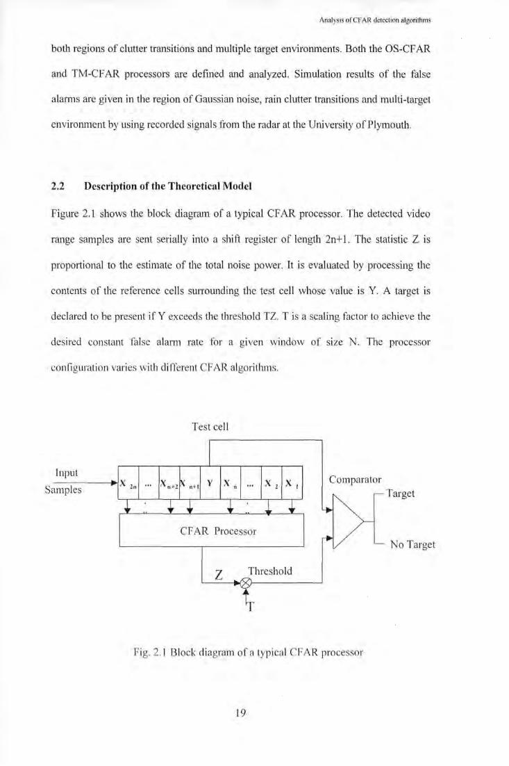
2.2 Description of the Theoretical Model
Figure 2. 1 shows the block diagram of a typical CF AR processor. The detected video
range samples are sent serially into a shift register of length 2n+ 1. The statistic Z is
prop011ional to the estimate of the total noise power. It is evaluated by processing the
contents of the reference cells suJTounding the test cell whose value is Y. A target is
declared to be present if Y exceeds the threshold TZ. T is a scaling factor to achieve the
desired constant fa lse alarm rate for a given window of size N. The processor
configuration varies with different CF AR algorithms.
Test cell
Input
S --1:------.JX l n .. . Xn+2 n+ l y X n amp es
Comparator Target
CF AR Processor No Target
z Threshold
Fig. 2. 1 Block diagram of a typical CFAR processor
19

,,
Analysis ofCFAR detection algorithms
..
CA: VI + Y2 GO: max(YI ,Y2) SO : min(Y I, Y2)
f------<~· z
Fig.2.2 Mean-level CF AR Processor
~, ~,
Sort and Select k-th cell
Fig. 2.3 OS-CFAR Processor
20
Analysis of CFAR detection algori thms
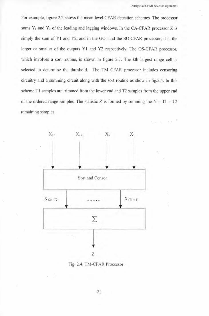
For example, figure 2.2 shows the mean level CF AR detection schemes. The processor
sums Y1 and Y2 of the leading and lagging windows. In the CA-CFAR processor Z is
simply the sum of Y l and Y2, and in the GO- and the SO-CF AR processor, it is the
larger or smaller of the outputs Y l and Y2 respectively. The OS-CF AR processor,
which involves a so1t routine, is shown in figure 2.3 . The kth largest range cell is
selected to determine the threshold. The TM _ CF AR processor includes censoring
circuitry and a summing circuit along with the so1t routine as show in fig.2.4. Ln this
scheme T l samples are trimmed from the lower end and T2 samples from the upper end
of the ordered range samples. The statistic Z is fonned by summing the N - T l - T2
remai ning samples.
X (2n-T2) ,,
Sort and Censor
r
z
Fig. 2.4. TM-CF AR Processor
21
x (TI + I)

Analysis ofCFi\R detection algorithms
In a homogeneous environment, it is assumed that the detected output for any range cell
is exponentially distributed, with probability density function (pdf1 as given by Van
Trees (I 968).
I < =~ l f(x) = -e ~~- ,x 2" 0.
2A.
Under the null hypothesis Ho of no target in a range cell and homogeneous background,
·;_ is the total background clutter-plus-them1al noise power, which is denoted by ll· Under
hypothesis I-1 I (presence of a target), A is ~1(.1 +S), where S is the average signal to total
noise ratio (SNR}of a target.
In a nonhomogeneous background, the reference cells do not follow a single common
pelf. During a single transition from a lower total noise background power level to a
higher level, the initial pm1ion of the reference cells have thermal noise only with A= p=
p0, and that the remaining reference cells arise from a clutter background with themml
noise so that here ), = .p= p0( I +C), with C being the clutter-to-them1al noise ratio
(CNR). The optimum detector sets a fixed threshold to cletennine the presence of a
target under the assumption that the total homogeneous noise power p is known. The
false alarm probability P10 is given by:
( - ) ~~ )
P = P[Y > Y IF-I ] = e 21' fo 0 0
where Y0 denotes the fixed optimum threshold. Similarly, the optimum detection
probability P d is given by:
22

Analysis orCfAR dclection algorithms
-);] I
P,, = P[Y > Yo I HI]= el.uii+Sl =[P;,,]i+.l'
Therefore, the statistic Z is a random variable whose distribution depends upon the
particular CF AR scheme chosen and the underlying distribution of each of the reference
range samples. Thus the processor performance is detem1ined by average detection and
false alam1 probabilities. As shown by Kassam ( 1988), Pra can be expressed by:
-I' -JZ
P E { 1 I 2;. d } E { _2--;;} , ·f ( T ) 1 = ~z - e y = ~z e . = w z -" z 2p . . 2p
Where Mz (.) denotes the moment generating function (mgf) of the random variable Z.
Similarly. the detection probability Pd is given by:
T P =M. [ ] " . z 2p(l + S)
There is an inherent loss of detection probability in a CFAR processor compared with
the optimum processor detection perfonnance in homogeneous noise background. This
is because the CFAR processor sets the threshold by estimating the total noise power
within a finite reference window. The optimum processor, on the other hand, sets a fixed
threshold under the assumption that the total noise power is known.
2.3 Analysis of Mean-Level CF AI~ Algorithms
Mean-level CFAR algorithms incorporate arithmetic averagmg to estimate the total
noise power. In this section, three such types of CFAR algorithms namely, CA-,00-,
and SO-CF AR algorithms are analysed. Their performance in homogeneous
backgrounds as well as in regions of clutter transition and multiple target environments
are· studied.
23

Analysis ofCFAR detection algorithms
2.3.1. Cell Averaging CF ~R Processor
In the CA-CFAR processor, total noise power is estimated by the_ sum of N range cells
of the reference window (Bar kat, 1990):
.I'
Z=l:X, !=]
Where Xi's are range cells sunounding the cell under test. The probability of detection
can be found as:
P,, =[I+ T /(I+ S)r"'
The constant scale factor T is computed by S=O:
T =(P )-IIN -I '"
In cases where the reference window no longer contains radar returns from a
homogeneous background. e.g. in the clutter edge, the statistical characteristics of the
reference cell is assumed to be independent. When the reference window contains r cells
from clutter background with noise power ~to( I +C) and N - r cells from clear
background with noise power Po. Then, the estimated total noise power is:
I X
z = 2:x, + Ix, ""zt +Z2 i=l ;=r+l
Since Z1 and Z2 are independent, the moment generating functioi1 of Z is simply the
product of the individual moment generating functions of Z1 and Z2 ~Rohling, 1983).
When the lest cell is from clear background, the false alam1 probability is:
24

Analysis ofCFAR detection ~lgorithms
P1, = (I + T 1(1 + C)r' (<I + T)'-N
When the test cell comes under a clutter background, the false alarm probability
becomes:
P,, =(I + rr' (I + T 1(1 +C))'-"'
In cases when the reference window contains two or more closely spaced targets, the
detection probability is given by Steenson ( 1968) as:
P,1 =[I+ ('I+ I)T 1(1 + S)r'.[l + Tl(l + s)f-x
Where r represents the cells in the reference window that contains the interfering targets.
C and I are assumed to be different noise conditions (themwl noise for C and clutter-
plus-thermal noise for I).
2.3.2 The Greatest Of and Smallest Of CF AR Algorithms
The greatest of(GO) CFAR is specifically developed to reduce the false alan11S at clutter
edges. The total noise power is estimated from the larger of the two separate sums
computed for the leading and lagging window (1-lansen and Sawyers, 1980), i.e.
n N
Z=max(Y"Y2 );}~ =2:X,;Y2 =IX, 1=1 i~ll+]
H-1 ( . I)' P_ · = 2(1 + T)-" -2' /1 +I- . (2 + T)-(u+•l
'" L..., "I( J)l '"0 1. n + .
The false alarm rate is found by computing the moment generating function of Z. The
detection probability P0 is found by simply replacing T with T/( I +S} The GO
25

Anal)>is orCf-ARdctection algoriUm1s
modification introduces additional loss of detection compared with the CA-CF AR
processor loss when the background is unifonn.
The smallest of (SO) CFAR is introduced to solve problems associated with closely
spaced targets leading to two or more targets appearing in the reference window. The
algorithm estimates the smaller of the sums Y1 and Y2, i.e. Z = min(Y 1Y 2) and the false
alarm probability is (Trunk, 1983):-
Myt(T) and MY2(T) are the moment generating functions of Yl and Y2 respectively.
This expression gives a very simple relationship between the perf01mance of SO-CF AR
and GO-CFAR. The GO-CFAR processor exhibits minor additional degradation in
performance compared with the CA-CF AR processor. On the other hand, perfonnance
of the SOcCFAR processor is highly dependent on the value of N. For small N the loss
is quite large compared with the other CFAR schemes, but decreases considerably for
increasing N. Weiss (1982) has shown that the additional detection loss in the SO-CFAR
scheme at Pt>, is 10-6 is !!dB for N = 4 but is only 0.7 dB at N=32.
Consider the special case where the lagging window has no1se values from clear
background and the leading window has noise samples from the clutter region. If the test
cell contains a sample from the clear background, the false alann probability is (Gandhi
and Kassam, 1988):-
n-1 ( · J)l J P1, = ( 1 +IT' + o +(I+ C)rr" - 2: ~~+' - ~· x o + r + --r('"'1 x [(I +er" + o + cr1 J
1= 0 J.(n+l). l+C
26

Analysis ofCFAR dclcclion algorilhms
As the reference window sweeps over the clutter edge, the detection rate of the GO-
CFAR is superior to that of both the CA and SO-CFAR.
In the presence of interfering targets, intolerable masking of a primary target occurs in
the CA- and GO-CFAR and this gets worse as the interference to signal ratio increases.
The effect is greater in the GO-CFAR than in the CA-CFAR. Tmnk ( 1978) shows that
the SO-CF AR has better perfom1ance in resolving multiple targets in the reference
window as long as all the interfering targets appear either in the leading or lagging
window. Suppose there is one interfering target in each of the leading and lagging
windows. The detection performance of the SO-CFAR will be degraded significantly.
This is due to the fact that there is one interfering target in each of the half window, the
noise power estimate includes power of the interfering target regardless of the specific
half window chosen. This results in an increased threshold leading to a decrease in the
overall detection probability.
2.3.3 Ordered Statistics (OS) CF AR Algorithm
The threshold of the OS-CFAR is obtained from one of the ordered samples of the
reference window. The range samples are first ordered according to their magnitudes,
and the statistic A is taken to be the kth largest sample, X(k). The detection probability
Pd can now be expressed as (Rohling, 1983 ):
The constant T is now a function of k. As k increases, T decreases accordingly. For
higher k values the noise estimate Z is one of the reference range samples that has
27

Analysis ofCFAR deleclion algorilhms
relatively large magnitude. Thus T decreases to compensate for this increase in Z to
maintain the design false alam1 rate at a constant value. As reported by Gandhi and
Kassam (1988), the OS-CF AR is perfonning better than the SO-CFAR especially for
smaller window lengths, although the OS-CFAR processor perfonnance is inferior to
that of both the CA and GO-CFAR.
Consider the situation where the reference window contains r clutter-plus thermal noise
cells each with power level (I +C)/2, the remaining N - r cells have the thermal-noise-
only with a power level of Y,. The following expression shows the false alarm
probability for the case when the cell under test is from the clutter-free region (Peterson,
Lee and Kassan1, 1988):
When the test cell is from the clutter region, the Pn, is obtained from the above results by
replacing T with T/( 1 +C). The k = N value cannot be used in practice due to suppression
of targets. Therefore, for k = N the noise estimate Z will be the highest ordered sample
which may contain the interfering target with high probability. The false alarm
probability will worsen in the clutter region, just after the transition, for decreasing k.
This is due to lower thresholds which in turn increases the false alarm rate.
Consider the OS-CFAR of window size 24 with k=21. In the worst case, there are 12
clutter plus thermal noise samples in the lagging window and 12 clutter free samples in
the leading window. The clutter samples occupy the top 12 positions of the ordered
28

Analysis ofCFAR detection algorithms
range samples and the total noise power estimate tends to be selected as the 91h largest
sample among the 12 clutter samples. Suppose the test cell contains a sample from clear
background. Then the threshold will be unnecessarily high, leading to a much lower
false alann rate, If the test cell is from a clutter background, the processor acts as if it
were an OS(9) processor of window size 12 in a homogeneous situation. The false alann
rate increases significantly.
In case of the presence of interfering targets in a reference window, the perfonnance of
the OS-CF AR processor is highly dependent upon the values fork. If a single interfering
target appears in the reference window of appreciable magnitude, it occupies the highest
ranked cell with high probability. If k is chosen to be 24, the estimate will set the
threshold based on the value of the interfering target. This results in an increase in the
overall threshold and leads to a target miss. If k is chosen to be less than the maximum
value, the OS-CFAR processor will be influenced only slightly for up to N ~ k
interfering targets. For example, if k is chosen to be 21. then the processor is able to
discriminate the primary target from, at the most, three interfering targets with little
degradation in detection performance.
Though the OS-CF AR exhibits some loss of detection power 111 homogeneous nmse
background compared with the CA and GO CFARs, its perfonnance in a multiple target
environment is clearly superior. By selecting k to be near the maximum, a false alam1
rate pcrfonnance close to that of the GO-CF AR is obtained. The detection .perfomwnce
of the OS-CF AR is independem of the location of the interfering targets in the reference
window while the SO-CFAR suppresses the primary target if the interfering targets are
located in both the leading and lagging window. In addition, the detection performance
29

Anal)'sis ofCFAR detection algorithms
of the OS-CF AR in homogeneous background noise is superior compared with the SO-
CFAR with k values approaching maximum.
2.3.4 The Trimmed-Mean TM CFAR Algorithm
The TM-CFAR scheme is similar to.OS-CI~AR in which the noise power is estimated by
a linear combination of the ordered range samples. It first orders the range cells
according to their magnitude and then trims T1 cells form lower end and T2 cells form
the upper end before summing the rest. The TM filter with symmetric trimming has been
used in signal and image restoration (Bovik, Huang and Munson, 1983). The statistic Z
of the TM-CFAR is given by:-
N--1;-T,
z = 2)', 1=1
The OS-CFAR and the CA-CFAR are special cases of the TM~CFAR with (T1,T2) = (k
- I, N - k) and (0,0), respectively. The false almm rate is given by Bednar and Watt
(1984) as:
,\'-/j -J;
P," = TI M,; (T) 1=1
T,l . ___ L (-1)7;-,
\ /1 1, 'I(T ')1 \I (T 1. . "\;'.J.l,-J. I' ,., ) = T, I ( N - T. - I) I ( N - T, - T ) X L. N - j'
I. I . I 2 t=O . - - - + T (N-T,-7~)
(/ i . M,,(T) = ,1 = 2, ... ,N- T,- T,
a, + T ·
30

Analysis ofCFAR detection algorithms
a, =(N-7; -i+I)/(N-7; -0_ -i+l)
The detection probability Pd is obtained by replacing T with T/( I + S). As the trimming
increases, T increases. Symmetric trimming can not offer advantages in perfonnance
over the other er: AR schemes in regions of clutter transitions. With symmetric
trimming, Z is given by the sum of the middle N - T1 - T2 range cells of the ordered
window. Consider the situation where the leading half of the reference window contains
cells from clutter-plus-noise background and the lagging half from clear background.
The noise power estimate Z will include samples from both the clear and clutter-plus
noise background. The corresponding threshold will not be high enough to regulate the
false alarm rate if the test cell contains a return from the clutter-plus-noise background.
As the upper trimming is increased with no lower trimming, the value ofT increases. On
the other hand, if the lower trimming is increased with no upper trimming, the value ofT
increases slowly and approaches the COJTesponding values for the OS-CF AR. In order to
be less sensitive to interfering targets, T2 should be different from zero. The actual value
of T2 depends on the maximum number of interfering targets present in the reference
window. The value of T1 should be small to attain good detection perfonnance in a
homogeneous background. However, if the primary concern is to follow clutter edges,
T1 should be large and T2 should be small.
2.4 Application of CFAR Algorithms
In this section, the quality of the CFAR algorithms is compared. For this purpose, two
40 microsecond sweeps of radar returns (containing both sea clutter and rain clutter
region) at Plymouth harbour were combined to form a 80 microsecond sea target
scenario in the video domain. The objective was to use this specific scenario to test
31

Analysis ofCFAR detection algorithms
the performance of the CF AR algorithms. The signal consists of 11 targets (including
multiple targets) and clutter transitions. The length of the radar sweep is 80
microseconds, which corresponds to a range of 12 Km. The video signal is sampled at
25 MHz, i.e. a range cell of 40ns corresponding to a range resolution cell of 6 m.
Figure 2.5 shows a plot of the sea target scenario with 11 targets identified.
Fig.2.5. Plot of the Sea Target Scenario for Testing the CFAR Algorithms 1.4
1.2
1
~ 0.8 0 > c 0.6 1 Q)
u :::l ......, 0.4 0.. E <:( 0.2
0
-0 .2
2
3 5 9
10
7
4 8
6 11
rain clutter sea clutter -04~--~----~--~----~--~----~--~--~
0 '10 20 30 40 50 60 70 80 Time in mi croseconds
Figures 2.6 to 2.10 show the CFAR thresholds for CA. GO, SO, OS and TM
algorithms. For the given sampling rate and range resolution cell size, the optimum
length of the CF AR window is chosen to be 120 (Holfele, 1998). To have a
reasonable comparison between these algorithms, the threshold of individual CF AR
algorithms have no fa lse alarms, i.e. the signal amplitudes in the scenario exceed the
CF AR threshold only for targets. The scaling factor T is set to 1.
32

Analysis ofCFAR detection algorithms
Fig.2.6. Sea Target Signal witll CA-CFAR Threshold 1.4
3 5 9 1.2
1
(f) 0.8 ~ 0 > c 0.6 ·-(].)
D :J
0.4 ....... 0. E <( 0.2
0
-0.2
-0.4 0 10 20 30 40 50 60 70 80
Time in microseconds
Fig.2.7 Sea Target Signal with GO-CFAR Tl1reshold) 1 .4 ~--~----~--~----~----~--~----~--~
1.2
1
B 0.8 0 > c 0.6 1 (].)
D
2 0.4 0. E <( 0.2
0
-0 .2
3 5 9
-0 .4 '------'----'-----'----'----- --'----'-----'-----' 0 '1 0 20 30 40 50 60 70 80
Time in mi croseconds
33

Analysis ofCFAR detection algorithms
Fig.2.8. Sea Target Signal wi th SO-CFAR Threshold 1.4
1 5 9 1.2
1
(f) 0.8 ....... 0 > c 0.6 Q) u :::J 0.4 ....... Q.
E <( 0.2
0
-0 .2
-0 4 0 10 20 30 40 50 60 70 80
Time in microseconds
Fig.2.9. Sea Target Signal witll OS-CFAR Threshold, 1<=80 1.4
1.2 3 5 9
1
(f) 0.8 ....... 0 > c 0.6 -Q) u :::J 0.4 ....... -Q.
E <( 0.2
0
-0.2
-0.4 0 10 20 30 40 50 60 70 80
Time in microseconds
34

Analysis ofCFAR detection algorithms
Fig.2.10 Sea Target Signal with TM-CFAR Threshold, T1 =40,T2=40) 1.6
c.n
1.4
1.2
1 ~
~ 0.8 ~ ~ 0.6 -~~ \ .a . .., E- o.4 ~
0.2
0
-0.2
3 5 9
10
7 4 8
-0 .4 '------'---'-----'---..._---'---'-----'---' 0 10 20 30 40 50 60 70 80
Time in microseconds
To determine the quality of a CFAR threshold, a crite1ion is established to calculate the
fitness of the threshold to the clutter and target environment. The criterion is based on
the assumption that there is no false alarm in the detection. This is perfonned by
summing the threshold crossings. i.e.
q = L[Y( i ) - Z(i) ]
for all i with Y(i)>Z(i), where Y is the magnitude of the range cell and Z is the
threshold. The following results are obtained for the five CFAR algoritluns.
35

Anal)~is orCFAR dclcclion algorilhms
Table 2.1 Quality of the CFAR Algorithms
CFAR Type Quality q
TM 17.0497
0S
so
CA
GO
16.0247
15.2160
12.0613
I 0,6400
TM-CFAR has the best quality. However, two targets that are embedded in clutters
are still missed. GO-CF AR has a worse quality than CA-CF AR. This is due to its
poor performance in the region of multiple targets.
2.5 Conclusion
The performances of five different CF AR processing algorithms in both homogeneous
and nonhomogeneous backgrounds have been analysed. The multiple target
environment and regions of clutter are used as examples for nonhomogeneous
backgrounds. A sea target scenario is used to indicate the variation of perfonnance
between the algorithms in a specific environment, i.e. multiple targets and clutter edges.
The detection performance of the CA- and GO-CF AR processors IS supenor m
homogenous background. However, the perfom1ance of CA-CF AR degrades
significantly in nonhomogeneous background. The false alam1 rate mcreases
considerably at the clutter edges, and target masking is experienced in multiple targets.
Although the false alann rate perfmmance of the GO-CFAR in regions of clutter
transition is better than that of any other mean-level CF ARs, the detection performance
36

Analysis ofCFAR detection algorithms
in a multiple target environment is quite poor. The SO-CFAR does not appear to offer
any advantage over the CA and GO CFAR. In addition to exhibiting high loss of
detection power in homogeneous background, the SO-CF AR is unable to resolve
multiple targets and to control the false alam1 rate at clutter edges. Yet, it has good
perfmmance in the multiple target environment when a clutter of radar targets appear in
the reference window.
The CF AR algoritlm1s based on ordered range cells have in general better overall
performance than the mean-level CF AR schemes (Kassam, 1988). The TM-CF AR may
have a slightly better performance in a homogeneous background for isolated targets
compared with the OS-CFAR. The performance of the OS-CFAR processor is relatively
unaffected if the clutter area is less than the window length as long as r, the number of
clutter samples present in the reference window, is greater than N - k. The false alarm
rate does not suffer considerably at the clutter edges if r $ N- k. On the other hand, the
CA and GO-CFAR exhibit fu11her false alam1 rate degradation if the extent of clutter
area is smaller than the window size. This is because the noise power estimate consists
of samples from clutter background as well as from clear background leading to overall
decrease in threshold. However, the performance of the OS-CFAR is highly dependent
upon the values of k. If k is chosen to be a high value, the noise estimate will set a large
threshold and it will result in target misses. Also, a low value of k will give excessive
false alarms. With regard to the TM-CFAR, again the choice of trimming factor T
affects the overall false alarm rate as well as the detection probability.
The experiment using the sea target scenario showed that the five CFAR algorithms
were unable to detect targets embedded in strong clutter. TM-CF AR with a good choice
37

Analysis ofCFAR delcclion algorilhms
of trimming factor could have a better perfom1ance in this specific case, However, two
targets were still missed. It is important to note that each algorithm aims to tackle a
specific problem in detection and it is obvious that no single CFAR algorithm is
adequate to solve problems in a complex detection environment, such as that in which a
YTS system is likely to be operated. A drawback on the CF AR algorithms is that the
decision is made only from the magnitude ofthe retum echoes (Li and Miller, 1997). To
have significant improvement in the detection of weak targets, more obvious
discriminating features must be identified and extracted. The following chapter will look
at the other characteristics of the radar signals for improvement in detection.
38
Charnctcristic of Radar Signals and FeatUre Extraction
CHAPTER THREE
CHARACTERISTIC OF RADAR SIGNALS AND FEATURE
EXTRACTION
3.1 Introduction
The limitations of the CFAR algoritlm1s in radar detection are mainly caused by their
static processing structures that they rely only on the amplitude infom1ation of the return
signal from targets and clutters. These algorithms are not suitable for a complex
dynamic environment such as the Hong Kong harbour. It is quite evident that the
detection capability of CFAR is vei)' limited under strong clutter background, as the
signal is embedded in the clutter which itself has a large amplitude. To provide a
significant improvement in the detection of weak targets, more obvious discriminating
features must be identified and extracted (Li and Miller, 1998). The radar detection
system may perfonn better when the characteristics of target and clutter are in line with
their predicted values. A wide range of targets and clutters will be received by the radar
systems and it is necessary to formulate descriptions about these signals at specific
times. In deciding whethc1: a target is present, there are factors other than the magnitude
of signal to be considered. The echo from the reflecting objects may consist of many
components of energy scattered from points over the surface. Their spatial and
correlation characteristics will vary as a function of time, angle of incident and
transmitting frequency. Radar returns of weak targets will have a closer temporal
correlation than those of a fairly strong sea clutter. Also, in the spatial domain, the
targets have some different features when compared with spiky clutter signals. An
effective approach to solve the problems in target detection is to develop algorithms
which are able to extract these discriminating features of signals in the radar return. With
39

Characteristic of Radar Signals and~Feature Extracrion
the recent development in the processing speed of computers, more radar information
can be handled in real time. This chapter will study the characteristics from radar return
signals in order to identify the features and extraction algorithms that can improve the
detection capability of a radar system.
3.2 Radar Cross Section
When a radar illuminates a target, the power that is backscattered or reflected back to the
radar is defined in terms of a measurable quantity, the target cross section. Since there is
substantial variation of the reflected power about the target for any given illumination
angle, an equivalent hypothetical target which re-radiates isotropically, is used as the
basis for measurement. The radar cross section (RCS), cr, implies an area of an isotropic
reflecting body which creates at the radar the same power density as does the actual
target.
Where I\ is the backscattered power at the target and P; is the incident or transmitted
power measured at the radar, and R is radar-to-target range. The RCS depends on the
characteristics of the target, namely the pennittivity and the pem1eability of the target
material. the target aspect angle relative to the radar, the shape and dimensions of the
target structural elements relative to wavelength, and on the polarization of the radar
receiving and transmitting antennas.
Some of the electromagnetic energy intercepted by the target is absorbed as heat and the
rest is scattered. Portions of the energy scattered in the direction of the receiving antenna
are received by the antenna and subsequently processed in the target detection system.
40

Characteristic of Radar Signals and Feature Extraction
Since radar targets such as ships, aircraft, missiles, and ground terrain have a variety of
fom1s and shapes, the use of mathematical models for smooth surfaces would lead to
incorrect calculations. As such, experimental measurements with the use of the target
itself or of smaller scale models form the basis of radar cross section calculations.
Measurement errors caused by parasitic reflections can be reduced by placing the model
in an anechoic chamber.
The target cross section fluctuates as a function of time. This is due to the scattering
effects that intercept the transmitted electromagnetic energy. A complex scintillating
target to a first approximation can be represented by an exponential distribution
(1-lovanessian, 1972). The radar illuminates the target once every revolution of the radar
antenna, with the duration of illumination proportional to the rotational speed of the
antenna, which is in terms of milliseconds. The target cross section used in the radar
equation is the average value of the cross section and the target scintillation is
incorporated in the probability of detection calculation.
The cross section of vessel type targets, as presented to the radar, is also a function of
aspect angle. lt can be seen initially that a vessel presents a larger physical area when
viewed from both sides rather than from the bow or the stern. A target viewed from the
sides may have an average cross section of 5 times larger than the same target in the
bow aspect.
A single value of RCS cannot be assigned to a target, e.g. a ship, as it will depend on the
aspect at which the target is viewed, both in azimuth and elevation, and also on the
polarization angle of the radar. These factors, combined with interference from different
41

Characteristic of Radar Signals and·Peature Extraction
scattering surfaces on the target, would mean that the RCS of the ship will fluctuate.
These fluctuations can be treated by finding the mean value of the RCS O"av and a
probability density function (PDF) p(a) to describe the variations about the mean. A
commonly used density function for random variables is the chi-squared variable with
two or four degrees of freedom, in the fom1s of:
I 1- ?. >
p(a") = -e a_.
am· 'a 4a (-~>
p(a) = -, -e a.,. (J- (/\"
a~O
For most of the surveillance radar, typical values of RCS (a .. ,.) that might be expected
are given in table I (Kingsley and Quegan, 1992).
Table 3.1 Typical RCS values for some common targets
Target RCS on Linear Scale RCS on Log Scale
Bird 0.001m2 -30dBm2
Cruise missile 1 o.otom- -20dBm2
Small boat I.OOOm 2 OdBm2
Cargo ship IO.OOOm 2 IOdBm2
Large aircraft I 00.000m2 20dBm2
Large tanker I 000.000m2 30dBm2
3.3 Clutter
Clutter is hard to quantify. and in many ground based systems it varies dramatically with
azimuth. The clutter seen by a marine radar depends on the sea-state and wind direction.
42

Chnracteristic or Radar Signals and Feature Extraction
Weather clutter is inherently variable and unpredictable. In spite of these difficulties, it is
imponant to have an overall appreciation of clutter cross sections for target detection.
Sea clutter is often distributed over a considerable area, unlike the point targets. Its
backscattering effect may be described in terms of a radar cross section density, cr0. If a
clutter area Ac produces an effective radar cross section O"c, then
ac a-o- A ,.
If the radar energy strikes the surface at an angle ~, a clutter area corresponding to one
resolution cell of the radar can then be specified. The cell's extent in the range direction
is detennined by the pulse length. A pulse duration of t seconds corresponds to a
transmit and return path of ct/2 metres. The equivalent distance along the clutter surface
is ctsec~/2 metres. The surface area lying within one resolution cell is therefore
The effective radar cross-section of the clutter area is
Suppose that a point target of area cr competes with clutter of effective area O"c in the
same resolution cell. If the power of the rettirn signals are represented by S and C
respectively. then the signal to clutter ratio is:
43

Characteristic of Radar Signals an~ Feature Extraction
S a 2a = =------
When the clutter is heavy, the clutter power will be much greater than the receiver noise
power. Hence the maximum range at which a target is detectable depends on the signal
to clutter ratio rather than the signal to noise ratio. If the minimum acceptable signal to
clutter ratio at the receiver input is (S/C)min, then
S' ? _a ( ---;-)min = R O C a 0c r sec 1/1 111" · H
From the above equation, it can be concluded that an effective way of improving the
signal to clutter ratio is to reduce the size of the radar resolution cell. This may be
achieved by reducing the pulse length, the antenna beamwidth or both. However, the
actual values of the clutter cross-section density cr0 depend heavily on the type of
surface, or terrain, and on the grazing angle ~· It is also affected by the choice or radar
frequency and the polarization. By taking a small grazing angles (~<I 0°) which are
widely used in marine radar, typical values of cr0 for city in X band, cultivated land and
sea are shown in the following table (Lynn, 1987).
Table 3.2 Typical values of clutter cross-section density
Horizontal Vertical
City -18dB -ISdB
Cultivated land -25dB -22dB
Sea -40dB -JOdB
44

Chnroctcristic of Radar Signals and Feature Exlraclion
The above quoted sea clutter values are typical of average sea conditions, in wind speed
of around 15 knots.
Rain or. other atmospheric conditions also produce clutters to radars. Such clutter is
usually quantified in tenns of an effective cross-section l1 per unit volume. Thus, if a
clutter volume Ye produces an effective radar cross-section O'c, then
0'. '7=V,or 0',='7I~
'
Now the radar resolution cell corresponds to a volume in space rather than a surface
area. Its extent is defined in range by the pulse length, in azimuth by the horizontal
bcamwidth 813 , and in elevation by the vertical beanl\vidth ~B· The approximate volume
of a resolution cell is:
Such types of volume clutter usually come from rain and cloud droplets. They are small
compared with the radar wavelength, and the cross-section presented by an individual
droplet is propmtional to the sixth power of its diameter. Heavy rain produces stronger
clutter than light rain or cloud, not only because there are more droplets per unit volume,
but also because they tend to be larger in size. Droplet cross-section is also proportional
to the fmuth power of the transmitter frequency. Therefore, the systems operating at
lower fl·equencies are much less susceptible to weather clutter. A typical relationship to
describe the effects of rain clutter on radar perfmmance is,
7/·~ 16 10-1' -1 '7"' .or·x -m
45

CharoctCriStic of Radar Signals and Feature Extraction
Where f0 is the transmitter frequency in GHz and r is the rainfall rate in mm/h. Given a
light rainfall of I mm/h, their cross sections as presented by two different wavelengths
(23 cm and 3 cm) at a range of 50nm (T = 211s, ell= I .SO, $u =l2°).are found to be 0.2m2
at J..=23cm and about 800m2 at /,=3cm.
3.3 Statistical Characteristics
Most of the random noise arises m the initial stages of the radar recetver. Their
behaviours during the target arrival period cannot be predicted. However, the statistical
distribution of random noise at the input to the intermediate amp I ifier can be assumed as
Gaussian, with zero mean value, which is mainly due to the thermal motion of electrons
in the early amplification stages. The probability density function ofGaussian noise with
zero mean is given by:
where lflo is the variance and lf/(:12 is the standard deviation. The random not se will
have a mean value close to zero. There is small chance that at a particular time the noise
level will be several standard deviations above or below the mean (Barton, 1988).
Most targets and clutters have a very complicated relationship to the cross section area.
and it is difficult to fonnat equations based on the physical dimensions. A complex radar
target (e.g. a ship) has many reflecting surfaces, such as the hull, accommodation, masts
and stern. Each of these contributes to the overall return signal, including the relative
phase as well as magnitude. lt is important to note that a speci fie target will not always
have the same cross section area as 'looked at' by the radar for a given incidence angle.
46

Characteristic of Radar Signals and Feature Extraction
Small changes in the direction of the incident wave can cause dramatic changes in the
effective cross section area of the target and these are very unpredictable. Also, clutter is
VC!)' difficult to define accurately, and it usually changes with environment and factors
such as wind and weather. Measurement of radar cross section of complex targets
requires readings to be taken at many frequencies, and with different polarisation. This
would lead to a massive database for a single radar band and limit the usefulness of
these data in radar performance analysis. These targets can be summarised in statistical
form and four statistical models were established based on probability density function
(Lynn, 1987). It was repot1ed that classes I and 2 are of Rayleigh type model and
con·espond to targets to which many scattering sources are added. Basically, all complex
targets having many comparable echo areas are very close to this model. For a target of
average radar cross section of a,,., the probability density function is of the f01m:
I a p,(a) = -exp(--), a~ 0
a,". a,u·
Classes 3 and 4 are more appropriate for targets having one dominant refiector, plus a
number of other, smaller renectors. The probability density function is of the fonn:
4a 2a p"(a) = -,-exp(--), a~O
0"-ar atH'
The intensity of the target echo depends on the aspect angle at which the target is
observed, the transmitter frequency and radar polarization. The target cross section area
changes with time, i.e. it varies between different sweeps due to aspect variation. These
variations will be present even when the vessel approaches the radar at constant bearing,
with the radar polarization and frequency remaining constant. This is caused by the
random movement of the vessel, the different propagation characteristics of the
atmosphere, performance of the electronic circuits in the radar equipment, and the
47

Characteristic of Radar Signals and Feature Extraction
variation in the transmission pattern of the radar antenna.
The Rayleigh scattering model can also apply to sea clutter if the sea is calm and the
range cells are fairly large. However, the range cells are relatively small in a short pulse
and high resolution radar. The size of individual sea waves may often be comparable
with a range cell, especially in a rough sea condition. Under these circumstances, the
distribution departs from the Rayleigh, with sharp peaks at the larger wave tops. Other
forms of distributions have been used ·to model sea clutler received by marine radars.
1ihese types of function have a longer 'tail' than the Rayleigh distribution. One of which
is the Weibullmodel with the fom1
where a and ~ are constants
Alternatively, the Log-nonnal, which has a longer 'tail', has the distribution
r v ' p(v) = -exp(-c5{ln[-]}-) V fJ
where p,y and 8 are constants.
The decision on which distribution is to be used depends on the sea state at that specific
moment. Yet the Log~normal distributions are best suited to rough seas. Moreau (1993)
has developed a model for sea clutter, which is a Rayleigh distribution modulated by a
Gamma distribution. The amplitude is represented by a compound K-distribution model:
p(v) = 2
h (bx/2)' K,_1 (hx)
!(v)
48

Chnractcristic of Radar Signals and Feature Extraction
where K, (x) v- order modified Bessel function
re X) Gamma function
x clutter amplitude
v shape parameter (function of sea-state, speed and direction of wind)
h scale parameter
The shape parameter v is a function of transverse resolution R, grazing angle $, wind
direction a and a coefficient k (k depends on polarisation) in the form of:
2 5 log v = -log r/J +-log R +a- k
3 8
Moreau (1993) had made simulations with this sea clutter model usmg a correlated
Gamma process. By estimating the high order statistics, he found out that, with v > 0.4,
simulated results fit well to the theoretical definition.
The volume cluller is usually caused by weather conditions such as ram and cloud
droplets. The reflectivity of volume clutter is quantified in effective radar cross-section
per unit volume. The rain and cloud droplets are usually very small compared with the
radar wavelength. They can nom1ally be described by means of Rayleigh modelling.
However, the radar cross section of droplets for cloud and rain is proportional to the
fourth power of the transmitter frequency. This causes the high frequency radars to have
more effects from the weather clutter. For shorter wavelength, the scattering prope11ies
may depart from the pure Rayleigh distribution.
49

Chamclcrislic of Radar Signals and Feature Extraction
Figures 3.1 to 3.4 show the recorded noise, target, sea clutter and rain clutter, and their
statistical distribution in a 2 microsecond time window. The window contains 50 samples of the
radar retum signal, which COITesponds to a distance of 300 meters.
Despite the fact that the magnitude of the random noise, sea clutter, rain clutter of these signals
are close to each other, it can be observed from their distribution that each type of retum echo
has its unique features. The random noise resembles a zero mean Gaussian function, with a
maximum number of occurrences at 0 volts. The target is characterised by the long tail which
extends by up to I volt. The majority of the sea clutter returns lie between 0 and 0.5 volt. The
rain clutter has similar characteristics to the random noise, except that the maximum is shifted to
around 0.5 volt.
To characterize the differences between these signals, the amplitude and period parameters in
the 4 microsecond windows are extracted. The waveforms contain a combination of several
frequency components and they exhibit a series of extremes over the time interval. A segment
boundary is declared each time that the waveform passes through a zero slope condition. The
segment amplitude is the absolute amplitude differences between the bounding extreme of the
segments, i.e.
A, = la, - a,-11
where A,= segment amplitude of the nth segment
a,= wavefom1 amplitude at the highest extreme of the segment
a,. 1 =waveform amplitude at the lowest extreme of the segment
The segment periods are the time differences between the lowest extremes of the
segments. This can be expressed as
50

Characteristic of Radar Signals and Feature Extraction
T,, = 1, -t,_,
where Tn = segment period of the nth segment
tn =waveform elapsed time at the firstlowest extreme of the segment
tn-1 =waveform elapsed time at the next lowest extreme of the segment
To sample the wavefonl1S, a trigger signal is activated whenever the waveform exhibits
a zero slope condition, indicating an extreme position. As such, direct extraction of the
waveform amplitudes (ao; a1, ..... a11 ) as the amplitude outputs of the monitoring circuit
can be achieved. The segment amplitude (A I, A2, ..... An) can then be calculated simply
by subtracting consecutive waveform amplitudes and taking the absolute values of .the
differences, The triggered sampling technique can also provide trigger signals at
waveform extremes, which are the segment boundaries. These signals may be used to
stimulate an electronic counter to retain its present count as an elapsed time
measurement. Consecutive elapsed time measurements (tO, t I, ........ ,tn) are then
subtracted to obtain the segment periods (T I, T2, ...... Tn).
The absolute differences in amplitude between these extremes are then accumulated, and
their mean and mean deviation are also calculated. The four wavefom1 parameters, ie.
the amplitude mean, amplitude deviation, period mean and period deviation are the
primary measures by which the wavefonn can be characterized statistically. The mean is
the standard sample mean, in the conventional statistical sense, and is simply the sum of
the sample values divided by the number of samples. The mean deviation, however, is
neither the statistically conventional variance nor standard deviation. As only a measure
of the average sample deviation from the sample set mean is required, the statistically
51

Characteristic of Radar Signals and Feature Extraction
standard quantities, which involve the calculations of squares and square roots, cari be
avoided to achieve the computational simplicity. The mean deviation is the average of
the absolute differences between each sample and the sample mean. These parameters
can be expressed mathematically as follows:
\"
D =~I A - Jv! IN tl L... I t1 _\
i=l
'"'· M, = LCI;}I N,
i=l
\'
M,= 't(A,)/ N, 1=1
X,
D = " I T - M 11 N I ~I I \
t=l
where,
Ma =amplitude mean,
Mt = period mean,
Da =amplitude mean deviation
Dt = period mean deviation
Ai =amplitude of the ith segment
Ti =period of the ith segment
Ns =number of samples (segments)
The period quantities are in temporal units of microseconds and amplitude units are in
quantities of volts. The statistical data of target sea clutter, rain clutter and noise, as
calculated by the author using the waveforms recorded at the Plymouth harbour, are
given in the following table:
52

Characteristic of. Radar Signals and Feature E:draction
Table 3.2 Statistical data of target, sea clutter, rain clutter and noise
Target Sea Clutter Rain Clutter Noise
Mean (amplitude in volts) 0.1952 0.2340 0.5880 0.0584
Deviation (amplitude) 0.2296 0.2014 0.1960 0.1060
Maximum (period in microseconds) 0.8 0.44 0.36 0.48
Mean (period in microseconds) 0.1704 0.1508 0.1584 0.1523
S. Deviation (period) 0.1550 0.1026 0:0905 0.0979
The noise has a comparatively low mean amplitude. This can be explained that the noise
is fluctuating randomly around zero and the sum of these amplitudes will be close to
zero. The rain clutterhas a comparatively high mean amplitude giving high peaks in the
radar receiver. The negative values of the amplitudes are due to the bias and offsets of
the amplifiers in the radar equipment. The amplitude deviation of sea clutter is small as
most of the amplitudes are varying along the means value. The mean period of the
window containing target(s) is large, which signifies that targets have a wider pulse
width when compared with noise and clutters. Such statistical characterization fonm the
basis for a discrimination system for target detection.
3.4 Correlation
The ability to detect trlrgets from signals coming from the receiver is largely depending
on the signal to noise ratio (SNR). Hence, it is impot1ant that the SNR is maximized.
The noise power is dependent only on the gain of the receiver, not on the shape of its
impulse response function. For fixed gain, the best SNR is obtained by maximizing the
response to the signal tem1. This is achieved by coiTelating the retum echo with the
transmitted pulse. The receiver can be regarded as a linear filter with impulse function
53

Characteristic of Radar Signals nnd Feature Extraction
h(t), and the output from the receiver, y(t) is therefore given by a convolution operation:
"' y(l) = u(l)*h(l) = Ju(r)h(l- r)dr
_.,
where 1 is a time variable and u is the input
According to the Cauchy-Schwartz Inequality (Kingsley and Quegan, 1992), the
maximum value of signal to noise ratio can be obtained by choosing h( r) proportional
to u( r + ( r" -I)) and h( r) is a reversed and shifted copy of u( r) where r" is the time
delay. Hence,
r
y(l) = Ju( r)u( r + r" -l)dr
where u( r) is the incoming signal
11( r + r" -I) .is a copy of u shifted to a duration of 1- r,,.
The product of the signal and its shi11ed version is integrated overthe ranges for which
the integral is not equal to zero. y(t) has the same shape as the autocon'Ciation function
of u(t). As t varies, the shifted u(l) will come to align with the incoming signal and then
out of alignment again. When they are fully aligned, i.e. 1 = r" , the maximum signal to
noise ratio will occur and the amplitude is given by,
r
y(l) = Ju 1 (r)dr 0
As such, the amplitude of the target after correlating with the transmitting pulse will be
greatly enhanced. The signal to noise ratio is much improved and this will facilitate the
target to be detected more easily.
54

Characteristic orRallar Sigrials and Feature Extraction
Fig. 3.5a shows a radar return with a target (at 18 microsecond) being contaminated by
noise. Since the transmitted pulse is rectangular in shape with a pulse width of 0.05
microseconds, the return echo will be stretched. The width of the integrating pulse can
be determined by trials. It is found that the best result can be obtained when it is around
I 0 times the transmitting pulse. Fig. 3.5b shows the result of integrating the product of a
0.4 micro second rectangular pulse by the radar return. It is obvious that the signal to
noise ratio is much improved and this will facilitate the target to be detected more easily.
New motion estimation algorithms in image processmg which exploit the motion
correlation of neighbour blocks in temporal and spatial directions have been presented
(1-lsieh, Lu and Shyn 1990 and Loui and Azimi-Sadjadi 1991 ). Winston, Yu, Meyer and
Byme ( 1995) and Chen, Deng and Zhuan (1995) have reported techniques for automatic
tracking and identification of moving targets using correlation algorithms. The targets
from the radar return will normally appear in more than I sweep in the same scan. The
same target will also appear in next scan within a certain limit of distance. depending on
the speed of the target. The degree of correlation will depend on the size and type of
targets. Large sized targets will be correlated in a greater number of consecutive sweeps
than those small sized ones. The speed of a vessel is relatively slow when compared
with the time between sweeps and it can be ignored in calculating the correlation, For
example, the vessel is moving at a speed of 15 nm/hr (27.78 km/hr) and the Pulse
Repetition Frequency (PRF) is 13001-lz (shmi/medium pulse).,i.e. one sweep takes 769.2
microsecond. The vessel only travels 0.463 mm. Also, taking the rotational speed of the
radar antenna is 20 rpm, one complete scan takes 3 seconds. The vessel travels 23.15
mm in one scan period. The conelation between the targets within consecutive sweeps
can be detennined by:-
55

m=l
c·.\ ... 1..,.1 (v) = L. v~ ... ,, v.~..,.~.~ ..... m=O
Characteristic of Radar Signals and Fcatun::·Extraciion
where C~ ~ (v) is the correlation of target points between n, and n+ I sweeps "tr' n·l
V~ • .~,. is the amplitude of nth sweep at time m
is the size of the correlation window
Random nmse is usually uncorrelated and thus can be removed after the first order
correlation process. Despite the fact that most of the uncotTelated noise is removed, there
is still some cotTelated noise appearing which may affect the target detection process.
The use of high order correlation method (Liou, 1991, 1992 and 1993) can provide a
better discrimination capability between clutter and noise. This is achieved by
cotTelating the cotTelated results ofN/N+I and N+I/N+2 to generate a new sequence of
radar signals.
Figures 3.6a, 3.6b and 3.6c show three consecutive sweeps of a radar retum with a time
frame of I 0 microseconds. The correlation of N/N+ I and N+ 1/N+ 2 are shown in figures
3.7a and 3.7b respectively. Figure 3.8 shows the effect of using high order correlation. The
noise is suppressed and the targets can be discriminated from the trace easily.
3.5 Spectral Chantctcristics
Target motion in range introduces a doppler shift of2v/A. relative to the transmitted catTier
frequency. As the target changes its velocity and heading, the spectral components are
shifted. The movement of the target and its elements, as well as yaw, pitch, and roll, cause
the spectrum of the received signal to fluctuate. The spectrum does not depend much on
target dimension and is detem1ined by the rate at which the range to different reflecting
56

Characteristic of Radar Signals and Fcati.Jrc Extraction
elements varies. Vmious techniques have been reported in detecting signals using their
frequency characteristics, e.g. low pass filtering, integration and matched filtering (Van
Trees, 1968). It appears that radar targets have distinct features in the frequency domain
compared with clutter and noise. Targets appear at some specific time of the radar sweep
and the corresponding changes in the immediate frequencies throughout the time sweep
may be of use in the detection of targets. Annstrong and Ahmed (1989) have modelled the
immediate frequency function for a broadband signal by considering an input of n
frequency varying spectral components.
By taking the square of the time derivative of the signal x(t), we have
., " I ' ) [x'(l)]- =I- A,- rv,- (1){1- cos[2(b, (/)]}
•=I 2 + other cross-multiplied terms
" x(l) =I A, cos[~, (I)]
i=l
where uJ;(t) denotes the immediate frequency function ~;'(t)
If a low pass filter is applied to the signal [x'(t)l2, it will suppress the tenns associated with
cos[2Nt)] and the other cross multiplied terms, so:
' J n I 1 2 [x (I)]- l, 1.r = I- A, rv, (I)
1=1 2
The low pass filter output of the square of the input is also calculated as follows:
57

, " I 1 [x(l)]· I,.N =L-A,
i~l 2
Characteristic or Radar Signals and Feature Extraction
The immediate frequency function w(t) can then be estimated as:
The nomwlisation element provides the weights of the individual spectral components to
calculate a reasonable estimate of the immediate frequency.
The detection of radar targets in the frequency domain requires the immediate frequency
at each time slot to be estimated. A moving window of a fixed number of range cells is
shifted through the entire sweep. The immediate frequency for each window is calculated
using the nonnalization technique as described. If the window size is made too large,
frequency changes for small targets may be missed. However, a window that is too small
will involve additional computation time as well as producing unwanted fluctuation of the
frequency function due to random noise.
The slope of the distribution of the immediate frequency (i.e. the rate of change) may also
be significant in detecting targets. A large slope will imply that there is a target embedded
in the high frequency noise. or that there has been an abrupt change in the frequency of the
noise. To remove any sharp slopes caused by random noise, the immediate frequency is
averaged over several samples so that short duration changes of slope can be filtered out.
So, in addition to considering the frequency response of returned signals the presence of a
target may be confirmed by examining the rate of change of the immediate frequency.
This can be achieved by differentiating the immediate frequency function and detecting
58

Chamctcristic of Radar Signats·and Feature Extraction
the slope change. Differentiation of a signal in the time domain is equivalent to
multiplication of the signal's Fourier transform by an imaginary ramp function, i.e. passing
the signal through a filter that has a response H( w )=jw .
The respective spatial and temporal characteristics of radar target signal and clutter are
different to some extent on the return sweep. The targets have a lower frequency spectral
component. The width of the distribution of clutter and noise is usually narrow and sharp,
and this characteristic can easily be identified in the immediate frequency distribution. To
detect these distinct features, thresholds on both frequency and width are applied to the
incoming signal. The threshold for the frequency must be chosen so that the majority of
the noise components are filtered, thus reducing the computation effort of the width
detection in the next stage. As for the width threshold, the number of samples in the
moving window contributes a crucial part in the value chosen. Further observation and
analysis is required in order to optimize this process. This would compare retums obtained
under various clutter, noise and target characteristics with respect to their width in the
immediate frequency function.
By looking at the amplitude alone, it may be difficult to discriminate the targets from the
noise and clutter. The signal can be conve11ed into the frequency domain by taking the
discrete Fourier transform of the sweep. New architectures of high throughput and real
time Fast Fourier Transfom1 processors have been developed for radar signal processing
(Bungard, Lau and Rorabaugh 1989). A trace of the Fourier transfmm for a window that
contains noise alone is plotted in Fig. 3.9, this will be used as a benchmark against which
to compare the frequency spectrum for traces which contain signals of targets. It can be
observed that the frequency distribution for the noise alone is fairly constant at all
59

Characteristic of Radar Signals and l:caturc E:\traction
frequencies. It was thought that targets would have some different features in the
rrequency domain when compared with noise. Figures 3.10 and 3.11 show the frequency
characteristics of the window containing target and land clutter respectively. It has a
smooth frequency distribution and is similar to the Fourier transform of a triangular wave,
while that of the land clutter resembles a sync function, i.e. the Fourier transform for a
square wave. The peak frequency components of the noise are equally distributed along
the whole frequency spectrum. Using these features for discrimination, it is possible to
develop the immediate frequencies of the radar return, which are able to extract the targets
from the noise and clutter in the background. Observation windows are established and
the magnitude of individual spectral components within each window is obtained by
taking the fast f'ourier Transform. The immediate frequency is estimated by means of the
nonnalization technique. Figure 3.12 shows a plot of the immediate frequency of the
return echo at various time frames during a sweep, The landclutter has distinct
characteristics of low variation in frequency and low frequency components. The target
has a constant slope in its falling and rising edges and a lower frequency. To determine the
threshold for the frequency and width of the detection algorithms, the immediate
frequency function for a frequency for a sweep with only random noise is used for
comparison and this is shown in fig. 3.13. To compromise in allowing for weak targets
against time spent processing data, and thus provide efficient detection, upper and lower
thresholds are set.
3.6 Conclusion
The characteristics of radar signals and methods for the extraction of features in the time
domain have been discussed in this chapter. During a full rotation of the radar antenna; a
variety of retum characteristics may be observed. For example, when operating in coastal
60

Charncteristic of Radar Signals and Feature E'traction
regions, very low clutter may be seen in the seaward sector and significant clutters due to
the land sea interface and reflections may be received in other sectors. Targets and clutters
have unique features in their statistical characterization over a finite window. These can be
extracted for discrimination purposes. Radar retum signals, which have been reflected by
different objects, possess unique features when correlated with other wavefonns. When
the received signal is correlated with a square pules of similar pulse width, the signal to
noise ratio is much improved. Radar pulses are transmitted at fixed time intervals and
correlation of the targets between different sweeps reduces the amplitude of random noise.
This is easily removed by the sweep to sweep con·elation process. The use of high order
correlation, which perfonns the correlation between correlated results of two consecutive
sweeps, further suppresses the partially correlated clutters. The time frequency
characteristics can also be used to achieve effective target detection. To study such
characteristics, the instant frequency value of the signal at any specific time of the sweep
is estimated using a normalization technique.
The statistical characterization, correlation, and time-frequency characteristics can be
extracted from radar wavefonns to determine if a target is present. In a very complicated
environment, e.g. boundaries between the sea and land, the sea clutter may have certain
similar characteristics when compared with the targets. However, it is unlikely to have
similarities in all these parameters, i.e. in a multi-dimensional space. These parameters
themselves are extracted from moving windows along the radar retum and can be fed into
an infonnation fusion process for making the final decision. Thus, the detection process is
not based solely on the magnitude of the radar echoes and will provide a more reliable
technique for discrimination in target identification and tracking algorithms.
61

Frg 3 1 a Random Norse of a Typrcal Radar Return 03r-------~------~------~----~
0 25
02
~ 015 \1' 1\ I\ '· A !li\ ~ 0 1 r·! I ·. /' t' ., \ I I / 'I - I I /I I I ' l t• I ~ 0 05 I I I I \j ';i \ I I I 2 I I \ 11
jO \~ \/ f\ 1 'd I -005 \ V u IJ I .o 1 I \ i 11
-015 ~ -02L-------~----~~----~~----~
1 5 2 0
08
~ 0 6 0 > s ~ 0 4 ~ a.
05 Trme rn mrcroseconds
Frg 3 2a Radar Return of a Man ne Vessel
I
. I \ I I
E <{ 02 1\'
/\ I I\ t~ ~~
\' j
\!\ .· 'I ' • I ~-J
\ • ! fo
1/',i 0
-02L-------~------~------~------~ 0 05 1 5 2
Trrne rn rnrcroseconds
Frg 3 3a Sea Clutter Srgnal 08r-------~------~------~----~
07
06
VI
~ 05
~ 0 4 2
~03 ' I <{ '
0 2 •i I/
01
I '
I\
'·' • <
/\ I ·.
1\ ·' \ I,. \ ,'\
; I I
'I '-•I I . /\/ 1/\ ... · V
OOL-------~------~------~----~ 0 5 I 5 2
T1me rn mrcroseconds
62
Characteristic of Radar Signals and Feature Extraction
Fig. 3.1b Statistical Distribution of Random Noise 30 r---~--~----~--~--~--~
25
! (]) u li5 20 :s
I u u
~ 15
I 0
Q;
I ~ 10 I ::l
\ z
5
0 '
-0.5 0 0.5 1.5 2 2.5
18
16
14 (I)
g 12 (I)
's t! 10 0
0 8 Qi
.0 E 6 ::J z
4
2
0 -0 5
Amplitude in volts
F1g 3 2b Sta~sncal D1stnbu1ion of a Radar Target
I f I I I
I\ ' I
I \ \ \
\ I i ' I \
i I ___ ' '. I
0 05 Amplitude 1n volts
1 5 2
F1g 3 3b Statrsllcal D1stnbut1on of Sea Clutter
25
25r---~--r-~----~--~----~----, ,A
(I) u c (I)
20
~ 15 u u 0
0
210 E ::J z
5
I
/ I i
I I
I I
I I I \ I I I \
I
\ I
I \ \ \ \ \ \
OL_~~~--~-----'~- ~-----~----~--~ -0 5 0 0 5 1 5 2 2 5
Amplitude rn volts

F1g 3 4a Ram Clutter m a Radar Retum
09
08
.g 0 7 >
= ~ 06 I
e I a. E 05 , <t: I
o4 \ I I I
0 3 I ! I'
02QLlL' ----~05------~-----1~5----~2
Time m microseconds
F1g 3 Sa A typical Radar Return with S1gnal8emg Embedded in Noise 06~--~--~--~----~--~--~
05
04
-0 4 '------'------'-------'------'-----'------' 0 10 20 30 40 50 60
T1me m m1croseconds
F1g 3 6a Radar Return m N Sweep 14.---~----~----~--~----~
1 2
-0 2 '----~------'-------'------'------_J
0 2 4 6 8 10 T1me m m1croseconds
Characteristic of Radar Signals and Feature Extraction
F1g 3 4b Statistical D1stnbut1on of Rain Clutter 16,---~---.--~----~--~---.
I\ Q) u c
14
12
~ 10 5 u V 0 8 0 Q; ~ 6 ::> z
4
2
0 -0.5
/
0
I \
I I I I
{'. ,I I , I I l \ i \ I \1 I
I ' \
j \ 0 5 1 1 5 2 25
Amplitude m volts
F1g 3 Sb The Radar Retum afler correlating with a square pulse 4~--~--~--~~--~--~--~
-2 '------'--------'-----'-----'-------'----' 0 10 20 30 40 50 60
T1me 1n microseconds
Fig 3 6b Radar Return m N~1 Sweep 14~--~----~----~----~---.
1 2
63

F1g 3 6c Radar Return m N• 2 Sweep 14 .-----~-----,------~----~-----.
-04L-----~----~------~----~----~ 0 2 4 6 8 10
Tirne in rn1croseconds
F1g 3 7b CorrelatiOn of N+ 1 and N+2 Sweeps 18
1 6
14 j
1 2 I Q) u e
tl,
a. E <( 08 Ql
> m 06 <D
~ 11 er 04
" I ~~~~ ,, 02 ' ' ' ~ If j.~ ' ': . I~ 1
... ··;.· Jr.'"~ . IJ, ~. ,~-.~· ,· ' ·' ' • lt \' " 11~ '1' o>l, • •I
0 ,. , ~.o. I j '• l\ 1.., •' '.-' \' ·"
-0 2 L-----~----~------~----~----~ 0 2 4 6 8 10
T1rne 1n mcroseconds
F1g 3 9 Frequency Spectrum for a Window With No1se Only 10 .------r------~----~------~----~
m o "0
-15
- 20L-----~------~----~------~----~ 0 2 3 4
Frequency 1n Hz
64
Characteristic of Radar Signals and Feature Extraction
Q) "0 a Ci E <(
"' > i5 a; cr
F1g 3 7 a Correla~on of Nand N+ 1 Sweeps 1 8.-----~------r>----~------~----~
1 6
14
-02L-----~----~------~----~----~ 0 2 4 6 8 10
Time 1n microseconds
F1g 3 8 Correlation of NJN+ 1 and N+ 1/N+ 2 Sweeps 35
3
25
2
1 5 I I I
!
'I 05 l ' '
0 \._ lU '------' -'~ .)
-0 5 0 2 4 6 8 10
Time 1n microseconds
F1g 3 10 Frequency Spectrum for a Typ1cal Target 15.------r------~-----r------r-----,
- 15
- 20L-----~----~~----~------~----~ 0 2 3 4 5
Frequency 1n Hz X IOe

F1g 3 11 Frequency Spectrum for a Window With Landclutter Target 25.--------.---.-------.-----.--------.,
Frequency m Hz
Fi~~O~ Immediate Frequenoes for a Typical Sweep With n01se on~ 3 ~~-~--.---.---~----.---~-.
o·--~-~-~~~~-~-~~
0 5 10 15 20 25 30 35 40 T1me 1n Microsecond
65
Characlcrislic of Radar Signals and Feature Extraclion
25 x 10Efig 3 121mmed1ate Frequencies for a Typ1cal Sweep
2 11
~ ~ !
~ 15 , I~ l{ ~ , d I :i5 ~ nr· hA ~ 1 ~V I " V'l' lL
0.5
o~~-~-~-~~-~-~~
0 5 10 15 20 25 30 35 40 Time 1n Microsecond

Data Fusion Techniques in Radar Signal Processing
CHAPTER FOUR
DATA FUSION TECHNIQUES IN RADAR SIGNAL PROCESSING
4.1 Introduction
l'vlethods for the extraction of useful infom1ation from the radar signal were developed and
discussed in the last chapter. The next step is to identify methods which can relate the extracted
infom1ation to a final decision on whether a target is present. Data fusion has been a new strategic
research field which deals with the incomplete and sometimes incoherent infonnation derived
from different sources. This is the case of many impm1ant application areas such as target
acquisition (Luperman, 1994), image processing (Zhou, 1994), feature extraction (Abdulghafour,
Chandra and Abidi, 1993), computer vision (Tahani and Keller, 1990), and defense systems
(Maloney, 1989). Processing extracted data requires a technique capable of addressing a very
demanding issue, i.e. making decisions in unce11ain conditions. Since the individual infonnation
extracted from the radar signals can be distorted, noisy and vague, adequate data fusion
techniques must be developed in order extract the essential information which is not recognisable
in any of the single sets of data. Hall (1992) provides an extensive overview and a description of
classical data fusion techniques. These focus on the identity fusion algorithms based on feature
extraction and identity declaration. One method of dealing with such task requires ideas from the
advanced research in machine intelligence. Knowledge-based approaches are able to perfmm data
fusion in intelligent multisensor instrumentation. However, imprecision represents a very critical
issue for such knowledge-based systems as they arc generally inadequate for dealing with the
intrinsic vagueness of input sensor data and very poorly suited to directly process input sensor
data (Russo, 1994). On the other hand, fuzzy systems and neural networks offer the best solutions
66
---------- --- -- ----
Data Fusion Techniques in Radar Signal Processing
to this type of applications (Kosko, 1992). Both fuzzy and neural network approaches, which
numerically process knowledge, are particularly well suited to manage uncertainty and are
becoming powerful technologies with a growing range of applications. This chapter describes
how these two teclmiques are used in the data fusion of the extracted features from the radar
signal and their comparison is also discussed.
4.2 FUZZ)' Approach to Data Fusion
The concept of fuzzy sets addresses problems in which imprecision is an inherent aspect of a
reasoning process. Fuzzy reasoning allows the processing of problems to be expressed in the fom1
of rules which resemble the mechanism of human decision making.· Indeed, one of the key
features of fuzzy logic is its ability to deal with the typical uncertainty which characterizes any
physical system (Zadeh, 1965). This is a very critical task because the infom1ation acquired from
different sources can be incomplete and even conflicting. Fuzzy networks are usually structured in
the fom1 of rules that pennit a clear understanding of their operation. Russo ( 1994) has reported
the fuzzy techniques represent a comprehensive framework for intelligent instrumentation that
deals with multisensory input data. One of this author's papers describes the development of fuzzy
algorithms for a microprocessor based servomotor controller (Li and Lau, 1989).
4.2.1 Fuzzy Set Theory
A fuzzy set A with an element x has a membership function of ~tA(x) and is in the interval
between 0 and I. If ~lA(x) is I, then the element is a member of the set. Alternatively, if ~tA(x) is 0,
then it is not. Consider a fuzzy set A with five elements, which have the membership function of
0.7, 0.9.1, 0.9,0.7. The element with a membership function of I is a full member of A. whereas
67

Data Fusion Techniques in Radar Signal Processing
the other are only part members. The membership function detennines the degree to which the
element belongs to the subset. If a fuzzy set A is defined as "around I 0 volts" on a scale from 9 to
12, it can then be described by the following:-
A = (0.7/8, 0.9/9, 1110,0.9111, 0.7112)
Where 0.7,0.9 and I are the membership functions and 8, 9, 10, !I and 12 are the universe of
discourse. The following three definitions form the basis of the fuzzy algorithms.
I. The union of two sets, A u 8, corresponds to the OR function and is defined by
p(A OR B)= max(p,,(x), Pll(x))
2. The intersection of two sets, An 8, corresponds to the AND function and is defined by
p(A AND B)= min(~tA(x), PB(x))
3. The complement of a set A corresponds to the NOT function and is defined by
p(NOT A)= I - ~tA(x)
To establish the fuzzy algorithms. it is necessary to interpret rules that are based on experience so
as to give the output values that cmTesponding to situations of interest. A fuzzy rule consists of
situation and action pairs. and they are expressed in IF and THEN statements. For example, if the
signal has a high amplitude and its pulse width is wide, then it is likely to be a target. Such a rule
has to be converted into a more general statement for application to fuzzy algorithms. First, the
qualitative statements must be quantized into linguistic sets such as, large, medium, small and
zero. The statement can then be converted into, 'If the signal amplitude is large and the pulse
width is large. then the possibility that this is a target is high'.
68

Data,Fusion Techniques in Radar SigrJal Processing
Having fommlated the rule in fuzzy tem1s, the next step is to define the membership functions of
the linguistic sets. The shape of the fuzzy set is quite arbitrary and depends on the user's
preference. Trapezoidal and triangular shapes are usually used because of simplicity. The
membership functions representing the decisions are weighted according to the corresponding
input statements. A pair of input parameters may fire more than one rule. To determine the value
of the final decision from these contributions, the centre of the summed area, which is contributed
by individual rules, is evaluated. This can be expressed in mathematical terms as follows:-
11 11
0 = L(J..l, X U, )ILJ..l, I I
where ~~ is the membership function, U the universe of discourse, n the number of contributions
and 0 the output.
4.2.2. Fuzzy Algorithms for Data Fusion in Radar Signal Processing
A radar signal at specific time frames can be identified as a member of a class of signals on the
basis of l'vl different features of the wavefom1. Suppose that all the available infom1ation is
acquired from N sweeps of the same scan. A fuzzy statement is formulated, which yields the
degree ofmcmbership m of the input data.
111 = { (~ 1 )or( F21 )or ........ ( F,, 1)} AND{ ( ~ 1 )or( F11 )or ....... ( F81 )} ...... AND{ ( F13 )or( F23 )or ...... ( F.v.11 ) }
Where Fij( I :::; i :::; N, I :::; j :::; M) is the jth feature extracted from the signal from the ith sweep. The
fuzzy connective logic OR is used to combine all the available infom1ation about the same feature.
It maximises all the information about the same feature coming from different sweeps. On the
69

Data fusion Techniques in Radar Signal Processing
other hand, the choice of fuzzy connective logic AND is used for linking information about all the
features makes the identification of a target. Then a fusion of information related to the same
feature but derived from different sources can be perfonned.
m, = {(F1,)0R(F21 ) .. .. .. .0R(F,," )}
The membership function of all contributions mj( 1 ~ j ~ M) can then be fused together to obtain the
final degree of membership.
m= AND{m , : j = 1, ........ , M}
Consider the task of identifying targets from a number of radar return signals recorded at the
Plymouth Harbour, each consists of 50 samples. It is necessary to write a set of fuzzy rules based
on the features of the input signals. To recognise the presence of the target, the features of mean
pulse width (w) and mean amplitude (v) from each signal are extracted using the method as
discussed in the previous chapter. The output is the membership function which shows the
possibility of the signal being a target. Table 4.1 shows the membership matrix table for the
membership functions.
Table 4.1. Membership Matrix Table
Linguistic sets Quantized levels
w (microseconds) 0.5 1 1.5 2 2.5 3 3.5 4 v (volts) 0.5 1 1.5 2 2.5 3 3.5 4 output 0 1 2 3 4 5 6 7
Large 0 0 0 0 0 0 0.6 I Medium 0 0 0 0 0.6 1 0.6 0 Small 0 0 0.6 1 0.6 0 0 0 Zero 0.6 1 0.6 0 0 0 0 0
70

Data Fusion Techniques in Radar Signai:Processing
The quantized levels for v and w are from 0 to 0.4 volts and 0 to 4 microseconds.
Nine fuzzy rules are formulated for this application.
I. If v is large and w is large then the possibility of signal being the target is large.
2. If vis large and w is medium then the possibility of signal being the target is medium.
3. If v is large and w is small then the possibility of signal being the target is small.
4. lfv is medium and w is large then the possibility of signal being the target is medium.
5. lfv is medium and w is medium then the possibility of signal being the target is smalL
6. lfv is medium and w is small then the possibility of signal being the target is zero.
7. lfv is small and w is small then the possibility of signal being the target is zero.
8. lfv is small and w is medium then the possibility of signal being the target is small.
9. lfv is small and w is large then the possibility of signal being the target is medium.
Rule I implies the ideal condition where a signal with both large amplitude and large pulse width is
received. The signal is likely to be the target. Rule 7 shows a condition where signal' amplitude and
pulse width are both small. There is high possibility that the signal is noise. These nlles are
developed based on the experience of observing the waveforms from detected targets. Suppose a
radar signal with a mean amplitude of 0.34 and a mean pulse width of 3.4 is applied to the fuzzy
network. According to the range specified, only rules I, 2, 4 and 5 will be fired, and the output
would be contributed by these four rules as follows:-
Q = 0.5 X 7 + 0.75 X 5 + 0.5 X 5 + 0.75 X J = 4
.8
0.5 + 0.75 + 0.5 + 0.75
71

Data Fusion Techn iques in Radar Signal Processing
It is important to note that in this specific input, no contribution is given by rules 3, 6 and 7.
Figures 4. 1 and 4.2 show the graphical representation of rule no. 5 and the output respectively.
Mean pulse width Mean amplitude
3.4J..LS 0.34v
Fig.4. 1 Graphical representation of rule no.5
3 5 7
4.8
Fig. 4.2 Determination of the output from a set of rules
72
Output

Data Fusion Techniques in Radar Signal Processing
Since the maximum quantized level is 7, the nonnalised value of the output is 0.68, which indicates
that the signal is likely to a target. A similar calculation is done on 6 signals that consist of four
targets and two noise data. The targets have a relatively low amplitude when compared with the
two noise signals. This makes the detection using amplitude infom1ation extremely difficult. One
of the noise data is having a wide pulse width. 1l1e objective is trying to test the integrity of the
fuzzy algorithms in these extreme conditions and the result is shown in table 4 .2.
Table 4.2 Testing Sets for Fuzzy Network
Features of input signals Desired Output Normalized Output Mean Amplitude Mean Pulse Width
0.40 3.2 target 0.76
0.28 4.0 target 0.71
0.34 3.4 target 0.68
0.37 4.0 target 0.64
0.38 1.8 nOISe 0.37
0.28 3.4 nOISe 0.55
It can be seen from the table that the targets have a high membership funct ion at the output. By
applying a co1Tesponding threshold to such membership value the targets can be extracted from
these radar signals.
4.3 Data Fusion in Neural Networks
Data fu ion combines information from several sources, typically sensors, towards a
representational estimate. For example, the different information extracted from a single sensor
73

Data Fusion-Techniques in Radar Signal Processing
can be combined to give a more reliable output. The fusion of various information can reduce
overall uncertainty and thus increase the accuracy with which the features are perceived by the
system. The information provided by different sources can also serve to increase reliability in
the case of error or failure of one information source. The complementary information from
multiple sources allows.different features in the system to be perceived ~Luo and Kay, 1989).
An artificial neural network can be defined by a set ofprocessing elements called neurons, a
specific topology of weighted interconnections between these elements, and a learning law
which updates the connection weights. Neurons provide non-linear input/output transfer
functions. Data fusion techniques that adopt neural networks have·a number of advantages. The
first is adaptive fusion inference in which neural networks can infer the relationship between
the desired fusion output and the multi-source input. The second is generalisation from an
incomplete set of information. This is useful when the information from an individual source is
noisy or distorted. The third is non-linear filtering of noise. Neural networks are nonlinear so
they can perform more complex functions than linear filters. The fourth is parallel computing,
since the neurons in neural network function in parallel and they can process information from
multiple sources simultaneously.
4.3.1 Neural Nctworl• ThcOIJ'
A neural network is an information processing system that operates in an intensely parallel
mode. It consists of highly interconnected neurodes that are connected by a large number of
weighted links, over which signal passes. A neurode receives input stimuli along its input
connections and translates those stimuli into an output response, which is transmitted along the
74

Data Fusion Techniques in Rndar Signal Processing
neurode's output connection (Caudill, 1992). The output signal transmits over the neurode's
outgoing connection and splits into a very large number of smaller connections, each of which
terminates at a different destination. Most of these outgoing branches terminate at the incoming
connection of some other neurode in the network, others may terminate outside the network
and generate control or response patterns. The mathematical expression that describes the
translation of the input pattern of signals at specific time frame to the output response signal
consists of a three-step process. First, the neurode computes the net weighted input that it
receives along its input connections. lt computes the value of Ij as shown below:
" I,= I li'.;X,
J=l
In this expression, I; is the net weighted input received .by neurode i from a total of n neurodes
in the network. The incoming signal from the jth neurode is designated by Xj, and the weight on
the connection directed from neurode j to neurocle i is designated by wu (Caudill, 1992). Once
the input signal patlern I is computed, all information about the amplitude of the input signal
will be lost. Depending on the values of the weights, a strong input signal arriving over a
weakly weighted connection may have less effect than a weaker signal arriving over a strongly
weighted connection. A negative weight will reduce the overall stimulation of the receiving
ncurode.
The translation represented by the neurode's transfer function consists of converting the input
signal pattern to an activation level for the neurode. The activation level of the neurode is
equivalent to the level of excitement of a biological neuron. In most cases, the activation
75

Dntn Fusion Techniques in·Radar Signr~l Processing
function is a sigmoid function, i.e. the activation is expressed by an S-shape curve. The
commonly used sigmoid function is:
.f(l) = I I _, +e
With a derivative of:
d~/~1) = .f(/)(1- f(l))
The exact form of the sigmoid function is not particularly important, however, the function
should be monotonically increasing and bounded with both lower and upper limits, In the case
of t{l), the minimum value of f(l) as I approaches negative infinity is 0, and the maximum
value off(l) as I approaches positive infinity is I.
The final step accomplished by the transfer function is to convert the neurode's activation level
to an output signal. Most commonly. this is achieved by setting the output signal to the
foiiO\ving expression:
/(/), if[f(i) > T] } )', = { 0. otherwise
T is a threshold value. The neurode's output is its activation level as long as that activation
value exceeds a given threshold.
When a neural network is presented with a signal pattern, each neurode in the input layer of the
network receives a small piece of the pattern. Each of the middle-layer neurodes thus receives
76

Data Fusion Techniques in Radar Signal Processing
the entire input pattern, but the pattern is moditied by its passage through the weighted
connections leading to the middle layer. Since the weights on the connections are typically
different for each middle-layer neurode, each of these neurodes sees a somewhat different
version of the input pattern than its neighbours do, i.e. it sees a projection. This results in a
variety of output reponses from the middle-layer neurodes, ranging from no output at all to
one, possibly with an extremely strong output. Figure 4.3a illustrates the physical connections
of a typical neural network.
Learning of the neural network is achieved not by modifying the neurodes in the network but
by modifying the weights on the interconnections in the network. The output of each neurode
is determined by a function of the incoming signals and the weights on the input connections to
the neurode. Learning consists of making systematic changes to the weights in order to
improve the network's response performance to acceptable levels. The network is provided
with an input stimulus pattern along with the corresponding desired output pattern. The
common learning law typically computes an error, i.e. how far from the desired output the
network's actual output really is, This error is then used to modify the weights on the
interconnections between the neurodes (Demuth and Beale. 1993 ).
4.3.2 Neural Networks for Data Fusion of Radar Signal
Neural network consists of parallel distributed processing elements that are interconnected by
links. By defining the associated weights for each of the interconnections, it is possible to
process data in a very rapid manner. This technique provides the potential to process radar
information in real time. The difficulty of choosing an appropriate neural network architecture
77

Data Fusion Techniques in Radar Signal Processing
Fig. 4.3a A typical neural network architecture
Output Response
Output layer
Middle layer
Input layer
Input signals
78

Data Fusion Techniques in Radar Signal Processing
for data fusion of radar signal processing is one of matching the problem domain with the
network features. This includes the problem size (i.e. number of input features and processing
elements, number of outputs), the form of data (continuous, time-varying, uncertain), and
incomplete knowledge about the system parameters.
The simplest format which can be applied to information fusion is a single layer network
(ligure 4.3b) whose weights and biases could be trained to produce a correct target vector when
presented with the corresponding input vector. The perceptron has a hard limit transfer
function (Caudill, 1992). Each external input is weighted with an appropriate W, and the sum
of the weighted inputs is sent to the hard limit transfer function, which also has a bias input.
The transfer function classifies the input vectors by dividing the input space into two regions.
Output vectors will be either 0 or I. The learning rule is applied to each neuron in order to
calculate the new row of the weight matrix and a new neuron bias. The learning rule will
converge to a solution in linite time if a solution exists. Vectors from a training set are
presented to the network one after the other. I r the network's output is correct no change is
made. Otherwise the weights and biases are updated using the learning rule. When an entire
pass of the training set has occurred without error, training is complete. At this time any input
training vector may be presented to the network and it will respond with the correct output
target vector. If a vector is not in the training set and is presented to the network, the network
will tend to exhibit generalisation by responding with an output similar to target vectors for
input vectors close to the previously unseen input vector.
79

Dala Fusion Techniques in Radar Signal Processing
The network first presents the matrix of input vectors and calculates the network's matrix of
output vectors. Then it will check to sec if each output vector is equal to the target vector
associated with each input vector. The training process will stop if all input vectors have
generated the correct output vectors for a specific set of weights and biases, or after a
maximum number of epochs. lfnot, it will adjust the weights and biases and then return to the
presentation phase. The mathematical model can be expressed as:
Wncw = Wold +~yx
where ~ = 0 if the perceptron's answer is correct
~=-I if the perceptron's answer is wrong
y = the perceptron' s answer
Consider a simple information fusion problem of 24 radar signals that are recorded by the
author using the radar at the University of Plymouth. The objective is to classify these signals
into targets and noise. To achieve this, both the amplitude mean and maximum pulse width
have already been extracted from the radar signals and these are served as input vectors to the
network. In the training process, a I is assigned to targets and 0 to noise. The input vectors for
the problem arc plotted in fig. 4.4. The targets are marked with an ;o' and the noise is marked
with a ;+'. A network with two inputs, i.e; amplitude and pulse width, and one neuron is
trained to distinguish between targets and noise. The initial conditions for the weights and bias
arc generated from a random numbers. The result of the training is shown in fig. 4.4 where the
network adjusts its weights and bias to classify the input space into targets and noise. A
boundary line separates the two regions. The final values of weights and bias were obtained
after training for 1700 epochs ( W = [219.5580 7.5843]; B=[-51.0778]).
80

..s:: ........ u
s (1) (f)
:::J Q_
Data Fusion Techniques in Radar Signal Processing
Fig. 4.3b A perceptron with two inputs
output y
Neurode
w2 w l
x2 Input x 1 input
Fig.4.4. Classification of Radar Signals Using Perceptrons 10~--~----~--~----~----~--~----~---4
8
+
+
2 + +
0
§ -2 (1)
z -4
-6
-8
-10 L---~----~--~----L---~----~--~--~ 0 0.05 0.1 0.15 0.2 0.25 0.3 0.35 0.4
Mean Amplitude
81

Data Fusion Techniques in Radar Signal Processing
Perceptrons are only good for solving real world problems when data is linearly separable.
However, it is seldom the case. The development of the back propagation training algorithm in
the 1970s and early 1980s demonstrated that training procedure was possible for a network of
three or more layers. A backpropagation network operates in a two-step sequence during
training. First, an input pattern is presented to the network's input layer. The resulting activity
flows through the network from layer to layer until the network's response is generated at the
output layer. Then, the network's output is compared to the desired output for that particular
input pattern. If it is not correct, an error is generated, which is propagated backward through
the network to the input layer. The weights on the interlayer connections are modified as the
error passes backward based on the learning rules. Changes in each weight and bias are
proportional to the pattern of the network's sum squared error. When the network is well
trained, a new input will lead to an output similar to the correct output for input vectors used in
the training. Such characteristic facilitates the training of a network on a representative set of
input/target pairs as well as obtaining good results for new inputs, without training the network
on all possible input/output pairs (Fincher, 1990).
Backpropagation networks often use the sigmoid transfer function, which generates outputs
between 0 and I as the neuron's net input goes from negative to positive infinity. The use of
the bias tends to increase the chances that the network can find an acceptable solution and also
tends to decrease the number of training epochs required. It is quite usual that the
backpropagation networks have one or more hidden layers of sigmoid neurons followed by an
output layer of linear neurons. Multiple layers of neurons with nonlincar transfer functions
allow the network to learn nonlinear and linear relationships between input and output vectors.
82

Dala Fusion Techniques in Radnr Signal Processing
Derivatives of error are calculated for the network's output layer and then backpropagated
through the network until the errors are available for each hidden layer. The change to be made
in a layer's weights and bias are calculated using the layer's error vectors and the layer's input
vector according to the backpropagation rule. Before starting the training process, all the
weights and bias must be initialised to small random numbers to ensures that the network is not
saturated by large values. Training the backpropagation network requires the selection of the
training parameter and application of input vector to the network input. Then both the output of
the network and the error are calculated. The weights of the network are adjusted to minimise
the error. The generalised rule specifies the change in a given connection weight as:
W; = p E f(l)
E is the error for this neurode, P is the learning constant (between zero and one). and !tl) is the
input to the neurode. The process is then repeated until the error or the convergence of the
entire network is to an acceptable level as specified.
Consider the same fusion problem in which a group of 6 radar signals ( 4 targets and 2 noise
signals) are input to the network for target detection. The backpropagation network is designed
and trained to discriminate the target from clutters. The network consists of one input layer
with 2 elements, one hidden layer with 2 neurons and one output layer as shown in figure 4.5.
Both the mean amplitude and mean pulse width are extracted from these 6 radar signals and
used in training the network. It will then be required to identify the target by responding a !
clement output vector. The network should output a I if there is target presented in the signal
83
Data fusion Techniques in Radar Signal Processing
and output a 0 otherwise. The maximum error of O,OS is used as the limit for the training. The
network completes the training after 1220 iterations. Once the network is trained, a testing set
is used to evaluate the performance of the network. The set consists of mean amplitudes and
mean periods extracted from 6 radar signals ( 4 targets and 2 noise signals) which are not used
in the training. Table 4.3 and table 4.4 show the training data and the testing result
respectively. From the table, it can be observed that the normalised outputs of the network are
0.9702 to 0.9788 for target, and 0.0154 to 0.0378 for noise signals respectively. As such, a
significant discrimination is achieved and the network is able to detect the targets from the
radar returns effectively in this example.
84

Data Fusion Techniques in Radar Signal Processing
Fig. 4.5 A three layer backpropagation network
Output Response
Output layer
Hidden layer
Input layer
Inputs
85

Data Fusion Techniques in Radar Signal Processing
Table 4.3 Training Sets for the Neural Network
Features of input signals Desired Output Mean Amplitude Mean Pulse Width
0.40 3.2 target
0.28 4.0 target
0.34 3.4 target
0.37 4.0 target
0.38 1.8 nmse
0.28 2.4 noise
Table 4.4 Testing Sets for the Neural Network
Features of input signals Desired Output Normalized Output Mean Amplitude Mean Pulse Width
0.34 3.4 target 0.9767
0.33 3.0 target 0.9702
0.24 3.0 target 0.9755
0.28 4.0 target 0.9788
0.4 1.7 noise 0.0378
0.29 2.0 nOISe 0.01 54
86

Data Fusion Techniques in Radar Signal Processing
4.4 Conclusion
Data fusion techniques in radar signal processing using both fuzzy logic and a neural network
have been discussed in this chapter. The performance of these methods is verified by applying
signals from live radar videos to the network and observing the results. Fuzzy and neural
systems do not require mathematical models to estimate functions from sample data. Neural
network theory includes the mathematical fields of dynamical systems, adaptive control as well
as statistics. Fuzzy theory adds probability, logic and knowledge base into these fields.
The architectures of neural networks are parallel and consist of many simple nonlinear
summing junctions connected together by weights of varying strength. it has been shown in
this chapter that even a simple network can perform interesting and useful computations in data
fusion of radar signals for target detection. Perceptrons can classify linearly separable input
vectors very well. However, the output values of a perceptron can take on only one of two
values due to the hard limit transfer function. If the vectors are not linearly separable, learning
will never reach a point where all vectors are classified properly. Backpropagation is slow
because of small learning rates and there are a large number of variables in multi-layered
networks. Yet, the multi-layer perceptron can perform linear or nonlinear computations. In the
example, a three layered backpropagation network can successfully identify the targets from
clutters as shown in table 4.4.
Fuzzy systems generally offer the advantage of a clear understanding of the operation as they
can structure the knowledge in a way that resembles human thinking. The objective of the
example is to recognise the presence of targets in radar signal. The pattern is composed of two
87
Data Fusio11 Techniques in Rndnr Signni·Pt"ocessing
features (mean amplitude and mean pulse width for each radar signal) whose relative strengths
are characterized by the corresponding membership function. The strength of each feature in
the signals is obtained to calculate the overall degree of membership of the available
information to the defined class of target. From these numerical values, the presence of the
pattern of targets is more clearly defined.
There are significant differences, as well as similarities, between neural networks and fuzzy
systems. Neural networks learn from the training data to recognise future patterns or fuse
future data to arrive at decisions based on knowledge or solve future computational problems.
Fuzzy systems start from highly formalised insights about the behaviour of the systems and
they learn from the associative rules to estimate functions or formulate control strategies.
Learning from examples requires the formulation of a knowledge base with a collection of
input-output pairs. In neural networks, a multilayer network is used as an approximation
framework and both weights and bias are modified in according to the selected algorithms. As
for fuzzy systems, fuzzy if-then rules are used to relate the linguistic or fuzzy variable, which
allows an approximated match between the input and the antecedents of the rules.
Fuzzy systems are suitable to be applied to areas where we can use people's experience or
knowledge to develop the fuzzy if-then rules. Since there is no mature guidance in fuzzy set
theory for the determination of the best shapes for fuzzy sets, different shapes for different set
points need to be studied to obtain an optimum solution for various input vectors. The amount
of overlap with the fuzzy sets affects the efficiency of the fuzzy controller. In the case of too
much overlap, many rules will be applied for a single set of input vectors, and the situation will
88

Da1a Fusion Techniques in·R<idar Signal Processing
not be represented accurately. If there is too little overlap, it will be difficult to derive the fuzzy
decisions. In addition, it is extremely difficult to formulate universal rules for a complex radar
target detection problem as the complexity changes at different periods. Therefore, neural
networks are more commonly used in this type of problem where a large amount of sample
data from simulated/live signals can be obtained and used as training sets for the network.
89

The radar syslcm and dala acquisilion
CHAPTER FIVE
THE RADAR SYSTEM AND DATA ACQUISITION
5.1 Introduction
The radar system selected for the implementation is a Racal-Decca 'Series 70' installed at
the roof of Fitzroy Building (University of Plymouth). The radar is located about 3,7 km
from the sea front and is 'looking at' the Harbour of Plymouth. It picks up targets of
ocean going vessels, as well as pleasure crafts. Both sea clutter and rain clutter are
detected by the radar under adverse weather conditions, The data acquisition system was
set up to record the raw radar video for analysis purposes. The recorded videos are then
imported into the computer where processing takes place. This chapter describes the radar
system and the effect of its characteristics in signal processing, as well as the
development of the data acquisition system to match the characteristics of the radar
waveforms.
5.2 The Radar Equipment
As stated in the service manual of the radar equipment, it includes an X-band transmitter
(93 80-9440 MHz) with a nominal power output of I 0 KW. The top unit is fitted with 4 feet
end-fed slotted waveguide aerial and the rotational speed is 25 rpm. lihe horizontal
bcamwidth and vertical beamwidth arc 2 degrees and 23 degrees respectively. The sidclobes
within I 0 degrees of the main beam are better than -23 dB. The aerial gain is.approximately
28 dB with horizontal polarization. The pulse repetition frequency and pulse widths are
2400Hz at 0.08 microsecond (short pulse), 1200 Hz at 0.3 microseconds (medium pulse)
90

The radar system and data acquisition
and 600 Hz at 1.0 microseconds (long pulse). The receiver is equipped with a low noise
front end with a noise factor of better than 7 dB. The intem1ediate frequency is centred on
60 MHz with I. F. bandwidths of25 MHz (short pulse) and 4 MHz (medium and long pulse).
The viewing unit uses a raster scan fom1at with 625 line/60 field per second and 2: I
interlaced. There are 4 planes of 512 x 512 pixels for the radar picture memory and I plane
of 768 x 576 pixels for the synthetic data memory [Racal-Decca 'Series 70' service
manual].
5.3 Parameters Affecting the Radar Signal and Maximum Range
The radar transmits a train of narrow pulses modulating a high frequency sine wave carrier
and detects the nature of the reflected signal when hitting an object. The parameters which
affect the reflected signal and the maximum range is discussed as follows:-
5.3.1 Beam Width
The vetiical beam width indicates the height of the beam effect within the vertical plane.
This parameter determines the minimum range which the target is 'seen' by the radar. The
horizontal beam width is measured in degrees and indicates the width of the radar beam in
the horizontal direction. In this case, the horizontal beam width is 2 degrees measured at the
half power point. This is not a particularly fine beam as beam width can go down to 0.5
degree for some sophisticated radar equipment. The horizontal beam width of the radar
signal transmitted from the antenna has a decisive meaning in the bearing accuracy.
Incorrect information will be indicated in cases where the distance between the two objects
is smaller than the width of the beam at that range. The targets would be seen by the radar as
91
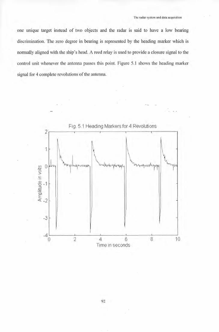
The radar system and dala acquisition
one uruque target instead of two objects and the radar is said to have a low bearing
discrimination. The zero degree in bearing is represented by the heading marker which is
nom1ally aligned with the ship's head. A reed relay is used to provide a closure signal to the
control unit whenever the antenna passes this point. Figure 5.1 shows the heading marker
signal for 4 complete revolutions of the antenna.
Fig . 5.1 Heading Markers for 4 Revolutions 2~------.--------.--------.-------.--------,
0.. E <{ -2
-3
-4L--------L------~~------~------~------~ 0 2 4 6 8 '10
Ti rne in seconds
92

The radar system and data acquisition
5.3.2. Pulse Repetition Frequency
The pulse repetition frequency (PRF) is the number of pulses transmitted from the radar per
second and it will limit the ma'<imum detectable range. Figures 5.2 and 5.3 show the PRF
for short pulse and long pulse. In the sh011 pulse, the PRF is 2400 Hz ( 416:67 microsecond)
which conesponds to a range of 62.5 km. For the long pulse, the PRF is 600 Hz ( 1667
microsecond) which cones ponds to a range of 250 km. The pulse width will affect the range
resolution of the radar. It is the time that the magnetron is active. In the radar used within
this work, the pulse width for shot1 pulse is 0.08 microsecond, which conesponds to a
distance of 12 meters, and the pulse width for long pulse is I microsecond which
conesponds to a distance of 150 meters. The pulse width affects the radar range; longer
pulse width tends to achieve a greater range due to the average power being higher.
However. it will have less range resolution, that is, it is unable to discriminate targets which
are less than 150 meters apart. For the s<m1e reason, the shot1er pulse width can achieve
better range resolution. Thus, shot1 pulse is usually used for close ranges and long pulse for
larger distance. Digitized radar video returns for both short pulse and long pulse are shown
in figures 5.4 and 5.5.
5.3.3 Transmission Power
During transmission, the peak power of the radar is I 0 KW and the transmitter is idle after
this pulse period. The average power or the radar pulse in walls is given by:
(Peak power (in KW) x Pulse Repetition Frequency x Pulse Width)/ I 000
93

The radar system and data acquisition
The average power is 1.92 watts for short pulse and 6 watts for long pulse. Apart from the
transmitted power, there are a number of factors which will affect the maximum radar
Fig. 5.2 . Pulse Repetition Frequency fo r S ho rt P ulse 6
5
4 .l:!J §;
3 c::: Q) -o .e 2 CL E
<t: 1
- 1 L---------~----------~---------J----------~--------~ 0 '1 2 3 4 5
Tt me in mt lliseconds
Fig . 5 .3 Pulse Repeti ti o n Frequ e ncy for L o n g Pulse 6
5
4 .l:!J C) >
3 s: Q) -o -~ 2 CL E <t:
1
- 1 L---------~----------~--------_J----------~--------~ 0 1 2 3 4 5
Time in milli seconds
94

The radar system and data acquisition
F ig . 5 .4 Six Sweep s of R adar Vi d eo for S ho rt P ulse 1~----~----~----~----~--~
o : ~ \~\\i\1t~~~~~ 1'<~~hl~li~W~ ·~IA\INJk\ ~~~~~~~\~ ~~~1~1 ~~~lil1\t'1 (f)
~ -0 .5 c::
{g -1 .a a. E -1 .5 -<
-2
-2 5
- 3 ~----~----~----~----~--~ 0 1 2 3 4 5
Time i 11 seconds
F ig . 55 Three Sweeps of Radar Video fo r L ong Pulse 0 .5 ~----~----.-------~----..---~
m -0 : INfj~~r·~l ~·w~~~~lll~~~~~r~~IW ~~~w~"~~ilf~\~~~~~~~~,~~~j ~ c:: -1 Q) -o ::::1
~ - 1 5 E ~
-2
-2 5
-3 ~----~----~----~----~--~ 0 1 2 3 4 5
Time i 11 seconds
95

The radar system and data acquisition
detection range. If the power of an omni-directional radar transmitter is denoted by P, the
power density at a distance R from the radar is equal to the transmitter power divided by the
spherical surface area of an imaginary sphere of radius R, i.e. P/4rrR2• The gain G of an
antenna is a measure of the increased power radiated in the direction of the target as
compared with the power that would have been radiated from an isotropic source. The
power density at the target from an antenna with a transmitting gain G would then be,
PG/4rrR2 . The target intercepts a portion of the radiated power and re-radiates it in the
direction or the radar and the re-radiated power is PGcr/4rrR 2 where cr is the radar cross
sectional area of the target. The power density of the echo at the radar receiving antenna is
then, PGcr/(4rrR2l The radar antenna captures a potiion of the echo power. If the effective
capture area of the receiving antenna is A. the echo power received at the radar is,
PGAcr/(4rrR2i. Antenna theory gives the ralationship between antenna gain and effective
area as, G = 4nA/),2. If the minimum signal that can be detected by a radar is:
PG 2 ,fu 2
Smin = (4;r)J(R'"" )~
then the maximum range for detection is
The above equation shows that if longer ranges are desired, the transmitted power must be
increased. This can be achieved by concentrating the radiated energy into a narrow beam
(high transmilling antenna gain), the received echo energy must be collected with a large
antenna apeiiure, and the receiver must be sensitive to weak signal (small Smin value).
96

The radar system and data acquisition
However, the minimum detectable signal and the target cross section area are both statistical
in nature and should therefore be expressed in statistical tem1s. Other statistical factors are
the meteorological conditions (rain, fog, sea clutter) along the propagation path. The
statistical nature of these several parameters does not allow the maximum radar range to be
described by a single number and a statement of probability that the radar will detect certain
type of target at a particular range must be specified.
5.3.4 Receiver Noise
Noise may originate within the receiver itself, or it may enter via the receiving antenna along
with the desired signal. If the radar is operating in a perfectly noise-free environment so that
no external sources of noise accompanies the desired signal, and if the receiver itself were so
perfect that it did not generate any excess noise, then there would still exist an unavoidable
component of noise generated by the thennal motion of the electrons in the receiver input
stages. The available thennal-noise power generated by a receiver of bandwidth Bn at a
temperature T (degrees Kelvin) is equal to, KTB 11 , where K=Boltzmann's constant= 1.38 x
I o-D joule/degree. Kingsley and Quegan ( 1992) and Barton ( 1988) state that the total noise
at the output of the receiver is equal to the thermal noise power obtained from an receiver
multiplied by a factor called the noise figure. The noise figure F of a receiver is given by:
F = ___ N_,.,_, -
K * 1;, * B, * G"
noise out of practical receiver
noise out of ideal receiver std temp T,,
97
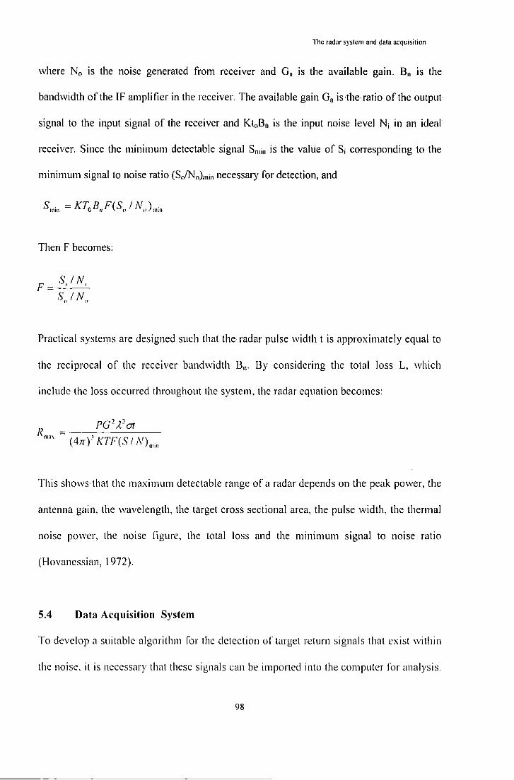
The radar system and ~ata acquisition
where No is the noise generated from receiver and G. is the available gain. Bn is the
bandwidth of the IF amplifier in the receiver. The available gain Ga is the ratio of the output
signal to the input signal of the receiver and Kt0 B, is the input noise level N; in an ideal
receiver. Since the minimum detectable signal Smin is the value of S; corresponding to the
minimum signal to noise ratio (SJNo)min necessary for detection, and
Then F becomes:
F = S, IN, S, IN,
Practical systems are designed such that the radar pulse width t is approximately equal to
the reciprocal of the receiver bandwidth B,. By considering the total loss L, which
include the loss occurred throughout the system, the radar equation becomes:
This shows that the maximum detectable range of a radar depends on the peak power, the
antenna gain, the wavelength, the target cross sectional area, the pulse width, the thermal
noise power, the noise figure, the total loss and the minimum signal to noise ratio
(Hovanessian, 1972).
SA Data Acquisition System
To develop a suitable algorithm for the detection of target return signals that exist within
the noise. it is necessary that these signals can be imported into the computer for analysis.
98

The radar system and'data acquisilion
This requires a data acquisition system which can record the radar video with minimum
distortion, as well as identify the bearing of each sweep so the both sweep to sweep and
scan to scan correlation can be performed. To cope with the wide band width of the
signals, a system with fast analogue to digital conversion rate is needed.
5.4.1 Sampling Rate
This parameter specifies how frequently conversions take place. A faster sampling rate
can acquire more points in a given time, thus providing a better representation of the
original signal. If the signal is changing faster than the sampling rate, errors will be
introduced into the measured data. When the data sampling rate is too slow, the signal
may appear to be at a completely different frequency due to aliasing. According to
Nyquist theorem, the sample frequency must be at least twice the rate of the maximum
frequency components. The frequency at one-half the sampling frequency is referred to
as the Nyquist frequency. Theoretically, it is possible to recover information about
signals with frequencies at or below the Nyquist frequency (Kuc, 1982). To sample the
radar signals when operating in shm1 pulse (which has a bandwidth of 12.5 MHz). a
sampling frequency of 25 MHz is needed. Video cassette recorders have been used to
record the raw radar videos. However, due to the limited bandwidth available (only
around 3 l'v!Hz), the video signal has to be compressed before being recorded. As such, a
lot of detailed information will be lost in the compression.
99

The radar system and dala acquisition
5.4.2 Resolution and Range
Resolution is the number of bits that the analogue to digital converter uses to represent
the analog signal. The higher the resolution, the higher the number of divisions the
voltage range is broken into, and therefore the smaller the detectable voltage change. For
example, if a 3 bit converter is used, it will divide the analog range into 23, or 8 divisions.
Each division is represented by a binary code between 000 and Ill. It is obvious that the
digital representation is not a good representation of the original analog signal because
information has been lost in the conversion. If the number of bits is increased to 16 bits,
the codes for the converter will be increased from 8 to 65,536 which can represent the
analogue signal very accurately. However, this will also require a larger space in the
random access memory of a digital system for storage. Taking the sampling rate as
25MHz, i.e. the interval is 0.04 microsecond per sample, then in short pulse, the period
for I sweep is 1/PRF, i.e. 417 microsecond. As such, there arc 417/0.04=10,417 samples
in one sweep and this would require I 0,417x 16=166,666 bits. The antenna rotates at 25
rpm, i.e. 2.4 seconds in one revolution. There are 5759 sweeps in one revolution and this
would require 960 M bits orl20 M Bytes of storage media. As such, the radar recording
system needs a large memory size as well as a fast data transfer rate to digitize the
waveform data into the computer for analysis.
5.5 Conclusion
The radar equipment that is available for use in this research is a general purpose marine
radar used in small commercial vessels. Selective sampling allows various weather
conditions including Plymouth rain clutters and sea clutters to be observed and recorded.
100

The radar system and dcua acquisition
The reflections from extraneous targets, such as those from nearbybuildings, are detected
by the radar in addition to those from vessels. It is the returns from vessels however, that
form the database for the analysis and implementing the feature extraction techniques. It
has been shown that the system requires a very special data logging system for recording
the waveforms, i.e. a high sampling rate and a large storage media. Also, the
instrumentation must be able to identify the bearing of each sweep so that analysis on
sweep to sweep and scan to scan correlation can be performed. One method is to divide
one revolution of the radar antenna into 4096 steps and encode each sweep with a sync
word at the zero range. A market survey has been undertaken by the author done and no
data acquisition system, which is suitable for this application, is available from
manufacturers. One company, Transas, has been developing a similar system using signal
processing chips from Texas Instrument. The equipment is still under development and
much of the processing will be undertaken by dedicated hardware. To overcome this
problem, a Tektronix TDS41 0 digitize oscilloscope is used as a data recording system.
The scope has a bandwidth of 1 OOMI-lz and is able to provide the sampling rate as
required by the radar signal. The internal memory in the scope is limited so only a few
sweeps can be recorded in one time. The number of sweeps will depend on the sampling
rate used. The recorded waveform is then input to a IBM PC via a GPIB interface.
Software from Tektronix, called the 'Wavestar' is used to acquire the data for fmiher
analysis. The details of the complete system arc discussed in the next section.
101

The Integrated Radar Detection System
CHAPTER SIX
THE INTEGRATED RADAR DETECTION SYSTEM
6.1 Introduction
The radar system described in Chapter Five provides the raw radar videos from the environment
in the vicinity of the antenna. A data acquisition system is then implemented to record the video
signal for analysis purposes. In order to identity the targets and clutters, the recording is done at
a specific bearing only. This is to ensure that the data can be compared with the visual scene and
the observation on the radar display. Windows of signals containing targets and clutter would be
extracted for feature identification. The features include amplitude mean and deviation, period
mean and deviation, as well as the maximum pulse width. The criteria for selecting these
features are also discussed in this chapter. Results presented in tables 4.3 and 4.4 indicated that
neural networks may be suitable for target detection and this work is now expanded. The
training procedure and the detection algorithms are discussed in detail in this chapter.
6.2 System Hardware
To record the waveforms of radar signals, the raw video, trigger signal and the heading marker
from the radar transceiver are input to the Tektronix TDS41 0 digitised oscilloscope, which has a
maximum sampling rate of I 00 MHz. The recording length is 50 points per division with a
maximum of 15000 points, For exan1ple, at the 2 microsecond per division range the time
interval for each sample will be 0.04 microsecond. Therefore, the total recorded length is 0.04 x
15000 = 600 microseconds. This corresponds to around 1.3 sweeps of raw video in short pulse,
0.3 sweep in long pulse. To increase the number of recorded sweeps in 15000 points, the
sampling rate must be reduced. For example, at the 20 microsecond per division range, the time
interval for each sample will be 0.4 microseconds. Therefore, the total recorded length will be
102

TI1e Integrated Radar Detection System
0.4 x 15000 = 6000 microseconds. This con·esponds to around 13 sweeps of raw video in short
pulse, 3 sweeps in long pulse. The data is transferred from the oscilloscope to the IBM personal
computer via a GPIB bus. The configmation is shown in fig. 6. 1.
Fig. 6. 1 Block Diagram ofthe Experimental Set Up
RADAR TRANSCEIVER
I lEADING MARKER ... GPIB
VIDEO ~
STORAGE INTERFACE IBM PERSONAL ... SYNC ... OSCILLOSCOPE COMPUTER
...
RADAR DISPLAY UN IT
To compare the recorded radar signal with the actual targets and environment, it is necessary to
identi fy the bearing of each recorded sweep. One way is to use the electronic bearing marker as
a trigger signal for the acquisition process of the oscilloscope. As such, the acquired waveform
conesponds to the video shown on the display unit as marked by the electronic bearing marker.
However, it was observed that the output signal from the electronic bearing marker was
embedded in the electronic circuitry of the display unit. A considerable amount of effort would
be required to trace the circuit diagram and build interface ci rcuit to extract the signal. Jt was
decided that the heading marker signal , instead of the electronic bearing marker, would be used
as the trigger signal. The heading marker signal can easily be taken from the transceiver output.
lt was observed however that the heading marker is pointing south and there is a large radar
shadow in that direction due to the nearby buildings. No targets can be seen in that sector to
around 4 degrees either side of it. To enable the bearing of the marker signal to be adjusted, the
103

The Integrated Radar Detection Srstcm
author designed and added a time delay circuit at the output of the transceiver. The objective is
to introduce a variable time delay to the arrival of the heading marker signal. Since the antenna
rotates at 2S rpm, one revolution will take 2.4 seconds. An RC time delay circuit with a resistor
of I k ohm and a capacitor of I 000 micro farad is used. This contributes a delay of I second and it
corresponds to a bearing of 360 x I /2.4 = ISO degrees. By adjusting the I OOk ohm resistor, a
delay of 0 to ISO degrees on the heading marker can be achieved. The arrangement is shown in
fig. 6.2. Adjustment of the resistor allows digitisation of targets that can be seen visually and
observed on the radar display.
6.3 Selection of Features to be Extracted from Radar Signals
In Chapter 3, the characteristics of radar signal have been discussed and features can be
extracted from the signals for detection purpose. However, it is impossible to extract all these
features for detection due to the computational time involved in the process. As such, it is
necessary to identify the features that are just sufficient for discriminating targets from clutters
with the minimum computational time required. Discrete fourier transfonn (OFT) or fast
Fourier transform ~FFT) technique is commonly used to assess the relative contributions of the
frequency components in a radar wavefom1 and convert them into the frequency domain. The
waveform can then be characterised according to the relative amplitude of the components.
While this method is effective and accurate, it is also computationally intense. Consider a
wavefom1 that consists of a fixed frequency component and a variable frequency component.
The objective is to identify when one of the possible combinations of frequencies occurs in a
particular sample. The mathematical representation is as follows:
A(t,n) = A1 sin[(2m!,,)+~,]+ A1 sin[(2mf,,) +~,]
where A 1 =peak amplitude of the fixed-frequency component,
104

The lnlcgralcd Radar Delcclion SySiem
A2 =peak amplitude of the variable-frequency component
fo =frequency of the fixed, frequency component
fn =frequency of the variable frequency component
~ 1 =initial phase of the fixed frequency component
~2 =initial phase of the variable frequency component
t = elapsed time
The Fourier Transfom1 can be used to identify the frequency components of the samples.
Despite the fact that both Discrete Fourier Transfom1 and Fast Fourier Transform can solve the
problem, the FFT takes advantage of powers of 2 relationships to achieve a transform with
reduced computational complexity, compared to OFT. In either case, the number of basic
mathematical computational operations (add, subtract, multiply and divide) is a direct function
of the number of samples. 1-lirsch (1991). stated this relationship as:
N, = N,1 (for the DFT) N, = 5N, log(N,) (for the FFT)
where No is the number of operations required and N, is the number of samples.
In view of the computational complexity of Fourier Transfonn, it is necessary to find an
alternative means to characterise the frequency domain similarities and differences of
waveforms without actually performing the transform. The process must use simple
computational methods to extract the fi·equency domain significance of the waveform without
actually transfonning the signals into the frequency domain. The statistical signal
characterisation method characterises the radar wavefmm not only as a function of the frequency
components but also as a function of the relative phases of its frequency components. The
characterisation method is used to associate waveforms to,different types in a high signal density
and real time environment. "J:he characteristics of radar wavefon11S can be manipulated with
105

The Integrated Radar Detection System
simple statistical mathematics to produce a set of numerical parameters for a given waveform. It
involves the division of a waveform into segments which are bounded by the extremes of the
waveform, As shown in chapter 3, the absolute differences in amplitude between these extremes
are then accumulated and their mean and mean deviation are calculated. Similarly, the mean and
mean deviation of the times between the extremes are also calculated. The five \vaveform
parameters, amplitude mean, amplitude deviation, period mean and period deviation are the
primary measures which are used for characterisation purpose. In order to extract the special
features of individual targets, the maximum period between extremes is also evaluated. The
parameters on periods are numerically very close to the reciprocal of the frequencies of the
components presented in the wavefonn. Therefore, the characterisation technique can determine
the frequency indirectly, which is significantly simpler than a Fourier Transfom1.
Computationally, this technique offers a considerable reduction in the number of operations as
compared to the more classical methods such as Fourier Transfom1 and Correlation. It simply
sums consecutive time segments and is divided by the number of segments. Hirsch ( 1992)
worked out the number of operations required as follows:
N, subtractions+ N, additions+ I division to calculate the amplitude mean
+ I subtraction + I division to calculate the period mean
+ N, subtractions+ N, additions+ I division to calculate the amplitude mean deviation
+ N, subtractions + N, additions + I division to calculate the period mean deviation
which gives a total of approximately 6 N, +5 operations. When continuous sampling is required,
another N, operations would be needed to accomplish the detection of maximum and minimum.
The technique requires fewer computational operations in comparison to Fourier Transfom1 or
correlation (both auto correlation, and cross correlation).
106

~ 0 > c Q)
"0 .3 0.. E <(
The Integrated Radar Detection System
Fig. 6.2 The Time Delay Circuit for the Heading Marker
+ 14 volt
1.4
1.2
1
0 8
0 .6
0 .4
0 .2
IK
1000 UF
RI /
To I leading Marker circuit
0 volt
Fig . 6 .3 Waveform of a Target in a 50 Samples W indow
0 l J
/ -0 .2 ~·
0 0 .5 1 1.5 Time in microseconds
107
2
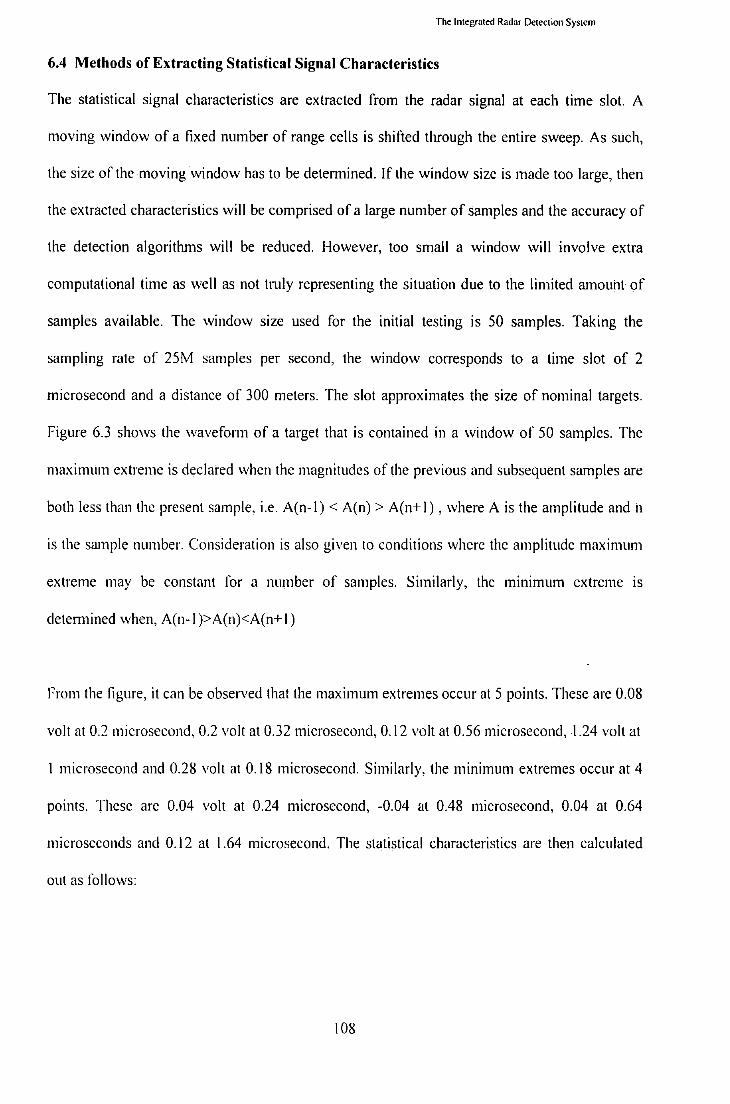
The Integrated Radar Detection System
6.4 Methods of Extracting Statistical Signal Characteristics
The statistical signal characteristics are extracted from the radar signal at each time slot. A
moving window of a fixed numbe~ of range cells is shifted through the entire sweep. As such,
the size of the moving window has to be determined. If the window size is made too large, then
the extracted characteristics will be comprised of a large number of samples and the accuracy of
the detection algorithms will be reduced. However, too small a window will involve extra
computational time as well as not truly representing the situation due to the limited amoui1t of
samples available. The window size used for the initial testing is SO samples. Taking the
sampling rate of 2SM samples per second, the window corresponds to a time slot of 2
microsecond and a distance of 300 meters. The slot approximates the size of nominal targets.
Figure 6.3 shows the wavefonn of a target that is contained in a window of SO samples. The
maximum extreme is declared when the magnitudes of the previous and subsequent samples are
both less than the present sample, i.e. A(n-1) < A(n) > A(n+ I) , where A is the amplitude and n
is the sample number. Consideration is also given to conditions where the amplitude maximum
extreme may be constant for a number of samples. Similarly, the minimum extreme is
detem1ined when, A(n-1 )>A(n)<A(n+ I)
From the figure, it can be observed that the maximum extremes occur at S points. These are 0.08
volt at 0.2 microsecond, 0.2 volt at 0.32 microsecond, 0.12 volt at O.S6 microsecond, 1.24 volt at
I microsecond and 0.28 volt at 0.18 microsecond. Similarly, the minimum extremes occur at 4
points. These are 0.04 volt at 0.24 microsecond, -0.04 at 0.48 microsecond, 0.04 at 0.64
microseconds and 0.12 at 1.64 microsecond. The statistical characteristics are then calculated
out as follows:
108

The Integrated Radar Detection System
Amplitude Mean = (0.08 + 0.2 +0.12 + 1.24 +0.28)/5 = 0.384 volts
Amplitude Deviation = (10.08-0.3841 + 10.2-0.3841 + 10.12-0.3841 + 11.24-0.3841 + 10.28-
0.3841)/5 = 0.3424 volts
Period Mean
Period Deviation
Maximum Period
= (0.6 + 0.4 + I )/3 = 0.667 microseconds
= (10.667-0.61 + 10.667-0.41 + 10.667-11)/3 = 0.222 microseconds
= I microsecond
Similarly, the statistical characteristics of eight sets of waveforms for targets (figures 6.4a to
6.4h) and eight sets of wavefonn for noise (figures 6.Sa to 6.5h) are shown in tables 6.1 and 6.2
respectively. The targets are returns from vessels in the vicinity of the radar and the noise
consists of both rain and sea clutters. The figures on the table show that each set of wavefonn
parameters is unique to a particular type of radar signals. Although there are similarities spread
across more than one parameter, the similarities seldom spread across all five parameters. From
these figures, different types of targets and noise can be extracted.
6.5 Neural Target Detection
The neural network's ability to learn, the fast on line processing ability and robustness of the
system indicates that it is appropriate to be applied in radar target detection. The method chosen
for the implementation of target detection is supervised learning using the backpropagation
leaming rules. This panicular methodology is chosen because they are simple to implement and
allow great flexibility in the structure of the system. The number of network inputs and the
number of neurons in the output layer are constrained by the information available and
requirements of the application. The number of neurons in the hidden layer(s) depend on the
designer. The more neurons, the more likely solution will be found. However, more neurons
109
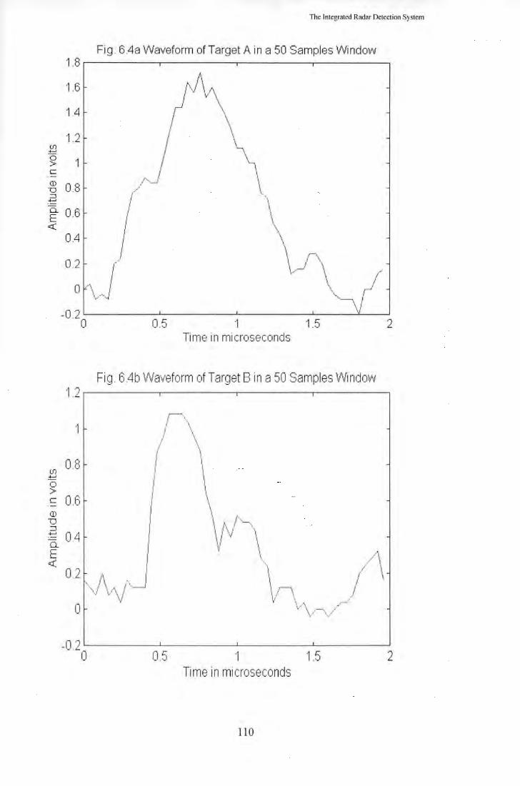
The Integrated Radar Detection System
Fig. 6.4a Waveform of Target A in a 50 Samples Window 1 .8.---------~--------~--------~------~
(f) ....... 0 > c
1.6
1.4
1.2
1
~ 0.6 <(
0.4
0.2
0.5 1 1.5 2 Time in microseconds
Fig. 64b Waveform of Target Bin a 50 Samples Window '1.2 .-----------,---------.--------.-----------,
tn ....... 0 >
'1
0.8
c 0.6 (]) "D ::J
....... 0.4 o._
E <(
0
-0 2 c__ ___ ____.J._ ____ ___j__ ____ L__ ___ ___J
0 0.5 1 1.5 2 Time in microseconds
110
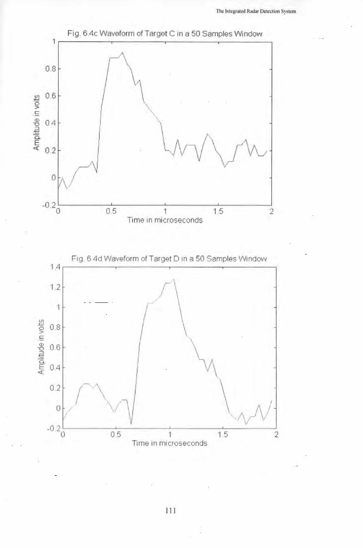
The Integrated Radar Detection System
Fig . 6.4c Waveform of Target C in a 50 Samples Window 1 .---------~---------.----------~---------,
0.8
!!] 0 .6 0 > c:
/1 (\
I \\ 11 ',
m ' -o 0 .4
~ I !" ~ <( 0.2
0 /\ / I /
-0 .2~--------~--------~--------~--------~ 0 0.5 1 1.5 2
Ti me in microseconds
Fig. 6 .4d Waveform of Target Din a 50 Samples Window 1 .4.---------~---------.----------.----------,
1.2
1
!!] 0 0.8 > c:
-8 0.6 ::::J ....... 0..
E 0 .4 <(
0.2
r I
I I
(~ .. __.\ I I \ .. , / I I
0 ,// \/ \/
......-\ I 1
I \ / \
\ \
\
\~ \/ ,, \
\ \ , I'· _!\ /
·-.1 \ / / oj
-0 2 ~--------~--------~--------~--------~ 0 0 .5 1 1.5 2
Time in mtcroseconds
1 I 1

The Integrated Radar Detection System
Fig. 6.4e Waveform of Target E in a 50 Samples Window 0 .8 ~------~--------~--------~---------,
0.7
/JV\ 0.6
(J) 0.5 ....... 0 ) I
> : \ c 0.4 { \ Q) I \ -a /V\\ ~~ I ~~ r I :::J 0.3 ....... 0. E J 1 ~ I \1 <( 0.2
~ \___ I 0.1 . I .!\ / 1\ I \
0 I V I
,;· I -0 .1
0 05 1 1.5 2 Time in microseconds
F1g. 6.4f Waveform of Target Fin a 50 Samples Window 0 .6~------~--~/' ----~---------.---------.
I' \ ... ,\/ .... \
05
04 (J) ~
0 0 3 > c
\ \
I \
I \ n / \
-' I ! l /ll ;"" I \ / 1
~ 0. 2 / \ I I / \ ,1\ .3 / \\ I \ ,,'' I . I I \ 0. / V\ _ _j I \
~ 0.1 \/ \ / \ I' 11 I \
0 LJ \ \l\.// -0.1
-0 2 ~------~--------~--------~--------~ 0 0.5 1 1.5 2
Time in mi croseconds
11 2

The Integrated Radar Detection System
Fig. 6.4g Waveform of Target G in a 50 Samples Window 0.6
0.5 ,~, / \
0.4 (\ r \ U1 \ ....... 0 0.3
~ > I I I c I ·-
\ Q) 0.2 , I \ ) D
\ \ ::J ....... \
Q.
\}\r~ \J \~ E 0.1
\ <( JV 0
\ -0.1
-0.2 0 0.5 1 1.5 2
Time in microseconds
Fig . 6.411 Waveform of Target H in a 50 Samples Window 12~------~~------~--------~--------~
1
0.8 U1 ....... 0 > c 0 6 Q)
D ::J
-~ 04 Q. .
E <(
0 2 I I
0\ \ /\/, ,/ \1 \ / \
•.·
/\/1 I '· I
'' I \ I • I / ....,
I \ I \
\ I
\ \ ·-,
\, \
\ 11
\ . ,~
V\ 1\1 ,----) ~~ I\ / \ , \/
-0 .2 L__ ______ __. ________ __. ________ ____._ ________ __,
0 0.5 1 1.5 2 Time in microseconds
113

The Integrated Radar Detection System
Fig. 6.5a Waveform of Noise A in a 50 Samples Window 0.4,----,----.-----,--------,
0.3
E3 0.2 0
~ /\ r\ ~ o.1 (V\ I \\ /\/ ~ V\1 ~ 0 I ~I
\}
-0.1
0.5 1 1.5 2 Time in microseconcls
Fig. 6.5b Waveform of Noise B in a 50 Samples Wi ndow 0.2 .------.-----.-----,-------.,
0.'15
-0 .15
-0 .2
-025~--~~---~--~~--~ 0 0.5 1 '1.5 2
Time in microseconds
11 4

The Integrated Radar Detection System
Fig . 6.5c Waveform of Noise C in a 50 Samples Window 0.25
0.2 {\
I \ / \
0.15 1
I \lj \ (f) 0.1 r~ ..__. 0
I '\ I I \ \r
>
~·~ I
.~ 0.05 I
Q) \1 "0 :J
0 ..__.
Cl. V 1\ \ E <t: -0 .05
-0 .1 (\ \I I L
-0.15 ~
-0 .2 1/
0 0.5 1 1.5 2 Time in microseconds
Fig. 6.5d Waveform of Noise Din a 50 Samples Window 0. 7 .-------,,....-----------,--------.-------,
0.6
0.5
~ 0.4 c
t'~.
/\ /r ....... \
;\I I \./ ~ 0.3 I' \
~ ~ l\ I \ / ~ 0
·2
/1 'v\ I 1~, 1 \ )I 0 .1 \,./ \------~ I \;\\l \
1 I \ r, o' V\1 V
-0.1 L....._ __ _____. ___ --~.. ___ ------'-___ ___.
0 0.5 1 1.5 2 Time in mi croseconds
li S

TI1e Integrated Radar Detection System
Fig . 6.5e Waveform of Noise E in a 50 Samples Window 0.4
~;V ;\ 0.35
0.3
I ~ (f) \ r ~ 0.25 I I \J v\ c \ / ·-
~ \J\; ~ 0.2 \\ ::J ......
\ o_
E 0.15 c::( v \
0.1 \ I
0.05
I 0 0 0.5 1 1.5 2
Time in microseconds
Fig. 6.5f Waveform of Noise F in a 50 Samples Window 0.2 r---- - -----.-----r------..----,
0.15 1\ i\ I I
1
1 \ I I I / l I
~I \I -0.15
-0 .2 I l -0 .25 '------------'-------'----'-----~
0 0.5 1 1.5 2 Time in microseconds
11 6
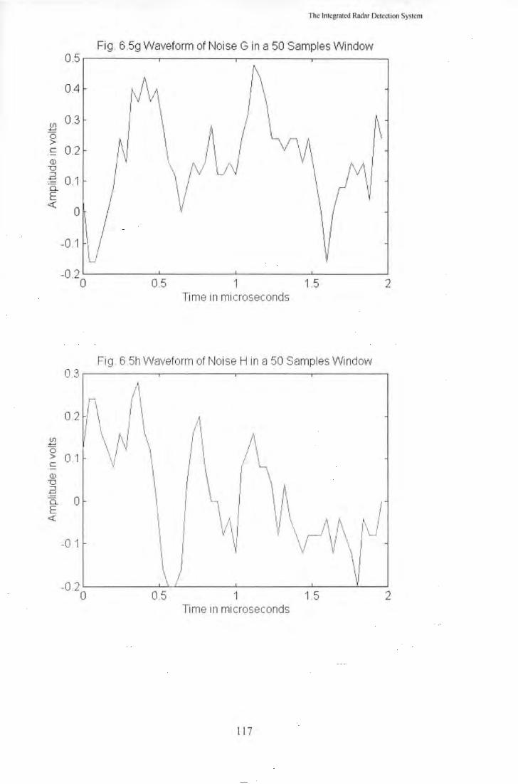
The Integrated Radar Detection System
Fig . 6.5g Waveform of Noise Gin a 50 Samples Window 0.5
(\ 0.4 rv~ /\ 0.3 I
1\ (f)
~i \ I~ I \,n,A ....... 0 > c 0.2 Q) t \ /, -)
\ \ ;v~ "0 yv v \ ::::l 0.1 .......
-0. E / I <{
0 I
I -0.1 -', I
u -0.2
0 0.5 'I 1.5 2 Ti me in microseconds
Fig . 6.511 Waveform of Noise H in a 50 Samples Window 0.3.--------.-----.------..-----.,
l\ r\ l \
0.2 ./ 11 ,' \ ~~ I I \ ( 11
(f) I \\ 1\j I I /1, ~ 1/1 \ I I /'\ ~ 0.1 'v '\ /' ( -\
i 0 \I\ I\~ I <{ I \ I \I \ ~ ~. .. I
',\ 11 ,/1~11 1\ \ I I l \ /\_J \ r--' \ l \ I ! 'v V \1 \ I \ -0.2 c__ ___ ____._--'-'-___ ___.__ ____ .____ _ ____._ _ __.
0 0.5 1 1.5 2
-0.1
Time in microseconds
117

The lntegraled Radar Dclcclion System
Tnble 6.l. Statistical Characteristics of Targets
Targets A 8 c D E F G H mean
Mean Amplitude 0.8743 0.3022 0.3467 0.3314 0.4145 0.2850 0.2800 0.3418 0.3970
Amp. Deviation 0.6694 0.2607 0.2104 0.3135 0.2003 0.1475 0.1600 0.3881 0.2925
Period Mean 0.2150 0.1382 0.1911 0.2057 0.1309 0.1956 0.1640 0.1354 0.1720
Period Deviation 0.1481 0.0939 0.0953 0.1388 0.0655 0:0988 0.1084 0.0847 0.1042
Maximum Period 0,5600 0.5600 0.3600 0.7200 0.2800 0.4000 0.4400 0.4800 0.4750
Table 6.2. Statistical Chamcteristics of Noise
Noise A 8 c D E F G I-I Mean
Mean Amplitude 0. I 343 0.0360 0. I 167 0.2520 0.3267 0.0360 0.2800 0.0920 0.1592
Amp. Deviation 0.1333 0.0735 0.0600 0.0706 0.1448 0.0533 0.0600 0.1000 0.0869
Period Mean 0.1143 0.1400 0.1229 0.1520 0.1233 0.1400 0.1354 0.1600 0.1360
Period Deviation 0.0539 0.0783 0.0459 0.1016 0:0542 0.0783 0.0577 0.0800 0.0687
Maximum Period 0.2800 0.3600 0.3200 0.4400 0.2800 0.3600 0.3200 0.3600 0.3400
118
The lnlcgralcd Radar Deleclion Syslem
means longer training times with larger weight matrices and bias vectors in the solution.
Initially, the test network consists of one input layer with 5 elements, one middle layer with two
neurons and one output layer. The five inputs are the amplitude mean, amplitude deviation,
period mean, period deviation and maximum period. These parameters for targets and clutter are
extracted from different radar returns for training purpose. In the initial training process, targets
are labelled as I while clutter and noises are labelled as 0.
To train a network, the five inputs are presented to the input layer of the network and the error
vectors are calculated. The maximum acceptable en·or is set within 5 percent of the desire value,
i.e. 0.05. If the sum squared en-or for all the training vectors is less than the error goal then
training stops and the corresponding vectors wi 11 be presented to the output layer. If the etTor
goal is not reached then the error vectors are calculated and back-propagated through the
network. Finally the weights are updated using the backcpropagation learning mle, i.e.
t-,W(i,j) = [JE(i)J(j) & 68(i) = fJE(i)
where 6 W is the weight change, I is the input vector E is the error vector and P is the learning
rate.
The learning rate specifics the size of changes that are made in the weights and biases at each
training sequence. Small learning rates result in long training times but guarantee that the
leaming process will not jump over valleys in the error surface. If a set of vectors from a radar
waveform, which is not in the set of input training vectors, is presented to a well trained
network. the network will try to exhibit generalisation in identifying whether the input vectors
belong to a target or clutter. To prevent the network from getting stuck in shallow minimum, a
term of 'momentum' is added into the network parameters. lt allows the network to respond not
119

The Integrated Radar Detection System
only to the local gradient but also to recent trends in the error·surface. The effect of momentum
is achieved by making weight changes equal to the sum of a fraction of the last weight change
and.the new change as given by the back-propagation rule. The mathematical tem1 is:
t..W(i,j) = mt..W * (i,j) + (1- m)fJJ(j)
where W* is the last weight and m is the momentum constant. The effect of the last weight
change is allowed to be mediated by a momentum constant. When the momentum constant is 0,
the present weight change is based only on the gradient. When the momentum constant is I, the
new weight change is equal to the last weight change and the gradient is simply ignored.
Typically the momentum constant is set to 0.95 which will be used initially for this
implementation (Demuth and Beale, 1993).
In order to detect any targets that may be constrained within each sweep, the 50 sample window
needs to be shifted along the complete sweep and analysis performed at each window. During
the shift. there arc samples being overlapped. Excess overlap across samples will increase the
number of windows to be processed and the measure processing time. Insufficient overlap could
cause a target to me spread across different \Vindows and reduce the chance of detection. If 25
overlapping samples are chosen, assuming that short pulse is used, the period for each sweep is
416.67 microsecond and the sampling rate is 25 MHz. This means that approximately 20,800
windows have to be analysed in each sweep. The number of overlapping samples is determined
by trial and this is discussed in the next chapter.
6.6 Conclusion
A general purpose marine radar is used in the implementation. The objective of the detection
system is trying to identify targets from the radar returns that are received from such radar
equipment. As a complete set of data acquisition system is not available, a continuous recording
120

The Integrated Radilf Detection System
of radar videos cannot be performed. By using the storage oscilloscope, a number of sweeps can
be recorded at one time. The number of recorded sweeps depend on the pulse width used, the
sampling rate and the record length selected. In order to compare the recorded sweep with the
image shown on the display, the heading marker signal is used as threshold for initiating the data
acquisition by the oscilloscope. A time delay circuit is added to delay the heading marker signal
so that the data recorded is in the region of interest. A neural network, that has been trained
using back-propagation, then provides the essential part of the detection system. A simple three
layer network is adopted for the initial implementation. The criteria for determining the initial
setting, e.g. window size, overlapping samples, initial condition, learning rate and momentum
constant are discussed. To prepare the training samples, hundreds of sweeps of radar returns are
recorded at different times under different environment e.g. rainy or stormy weather. Also,
different types of targets such as fishing boat, sailing yacht, cargo vessel and passenger liners are
recorded. Hundreds of representative windows are extracted from these sweeps and various
statistical characteristics of these windows are calculated. These values provide the training data
for the neural network. The training, testing and verification of the detection system will be
discussed in the next chapter.
121

Training, Testing and Verification of the Radar. Detection S)'Stem
CHAPTER SEVEN
TRAINING, TESTING AND VERIFICATION OF THE RADAR DETECTION SYSTEM
7.1 Introduction
Over two hundred sweeps of radar data were recorded using the data acquisition system as
described in the previous chapter. Windows containing targets and clutters were extracted from
these signals for training purposes. Initially, the mean amplitude, mean amplitude deviation,
mean period, mean period deviation and maximum period are evaluated from the windows. The
distribution of these parameters for both target and noise are discussed. Then the neural
detection system was fomllllated using the backpropagation techniques. The training algorithm
calculated and minimized the cost function or error value. The anticipated perfonnance of the
system can be considered to be improved if the error function has a reduced value. The error is
computed in each training cycle of the data set and is summed at the end of each pass through
the patterns in the training set. When the detection system has been trained, new sweeps of data
are used to ascertain whether the network can detect a target with the unseen data. The author
used Matlab together with the neural network tool box (from Math Works Inc.) to develop the
software for the implementation.
7.2 Feature Extraction from Radar Sweeps
To fonnulate the detection system, the first step is to obtain samples of targets, noise and clutter
in a 2 microsecond window, which consists of 50 samples at a sampling frequency of 25 MHz.
Targets close to the heading marker were first identified on the radar display. When the target
just passed the marker, the digital scope would be triggered to acquire the sweep and the range
of the target from the radar transmitter was measured. The target would then be identified from
122

Traini~g. Tcsling and Verification of the Radar Detection System
the data recorded and the window extracted as one of the samples. Noise was also present in all
the returns and this was extracted from the same sweep when targets were recorded. Rain.clutter
was recorded when heavy rain was observed in the region of the heading marker. There were a
number of occasions which gale force winds were encountered in the Plymouth area during the
data recording periods. Sea clutters were observed in closed ranges of the radar and the scope
was triggered to acquire such signals in the vicinity of the heading marker. To ensure that no
targets existed in the recording of noise and clutter by chance, the gain; sea clutter and rain
clutter control of the radar display unit were adjusted to see if targets were presented in the
vicinity from the radar screen. Also, the record was carefully checked for any targets that were
embedded in the noise. Initially, I 00 samples for targets, 50 samples for noise, 50 samples for
rain clutter and 50 samples for sea clutter were recorded, i.e. a total of 250 samples. A Mat! ab
program was written to calculate the five parameters from these samples. These include mean
amplitude, mean amplitude deviation, mean period, mean period deviation and maximum
period. The distribution of these parameters for targets, noise and clutter (rain and sea) is plotted
(figures 7.1 to 7.5).
Traditional radar detection system has been using amplitude as a discrimination feature. From
the distribution on mean amplitude (Fig.7.1), a large overlap between target, noise and clutter is
observed. There were instances where the clutter had a very large amplitude, especially during
the rain clutter environment. If a threshold is determined based on this amplitude distribution,
large false alann rate and low detection probability would result. Distribution of amplitude
deviation (fig 7.2) shows a better discrimination feature. The majority of the noise and clutter
had a very low amplitude deviation from the mean and is independent of the type of clutter. This
is due to the fact that the amplitude of noise and clutter tend to be more evenly spread in the
window·, whereas, for targets, a sharp rise in amplitude usually occurs. A variation of the
123

Training, Testing and Verification ofth~ Radar. Detection System
window size would have an impact on the value of the amplitude deviation. The selection of the
window size will be discussed in section 7.3.
Figures 7.3 to 7.5 show the parameters related to the period of return signals. The noise signals
are mainly spikes with a very fast rise and fall time. They consist of large high frequency
components that cause the width of the pulse to be much narrower than those of the targets. The
system detects the period between the consecutive negative extremes as an indication of the
width of the pulse. The mean period of each window was evaluated and shown in fig. 7.3. The
use of negative extremes (described in section 6.4 of Chapter 6) as detection criteria is a very
effective way of detem1ining the pulse width of individual pulses in a radar retum. An ideal
target would be one which has only two negative extremes, i.e. at the beginning and the ending
of the pulse. However, not all targets belong to this category. The width of the pulse would be
reduced if the number of detected negative extremes is increased. As such, some overlap still
exists in the distribution of the mean period, the period deviation and the maximum period. The
majority of the noise and clutters have a narrow pulse width and their deviation from the mean is
small, as shown in fig. 7.4. ·rhe maximum period signifies the width of a specific pulse which
has a maximum value in a window. This is useful in the identification and classification of a
possible target in the window.
Fom1 the graphs provided, it is observed that it would be a difficult task to discriminate the
target tl·om noise and clutter based on any one of the statistical characteristics. However, it is
impor1ant to note that redundancies may spread across more than one parameter but such
redundancies will seldom spread across all the five parameters to a degree that may be
inseparable by computational techniques. The spread of these five parameters for three targets
and three noise samples is shown in fig. 7.6. Examination of these distributions and spreads
124

Training, Testing and Verification of the Radar Detection System
show that targets nonnally have a larger amplitude and period than noise. However, there are
occasions where noise may also have similar characteristics in either amplitude or period, e.g.
noise 2 has similar features to target 3 in both mean period and period deviation. Yet, they can
still be discriminated by the amplitude parameters as well as the maximum period. Noise 3 has a
larger mean amplitude than targets I, 2 and 3, however its amplitude deviation is much smaller
than those of the targets. Therefore, it is necessary to include both amplitude and period
parameters for feature discrimination in the detection system.
Fig.7 .1 Distribution of Mean Amp litude
Q) 16 (..)
r:::: 14 Q) ... 12 ::l (..)
1 0 (..)
0 8 -0 6 ... Q) 4 .c E 2 ::l
0 z c:,<:::l "<;::)
<;::)· <;::)·
Mean Amplitude in Vo lts
Dtarget • noise D clutter
Fig . 7 .2 Distribution of Amplitude Deviation
Q) 45 (..) 40 r:::: Q) ... 35 ::I 30 (..) (J
25 0 - 20 0 ... 1 5 (I)
.c 1 0 E 5 ::I z 0
c:,<:::l <;::) ·
"C) C) ·
"VC) C)·
':)C) C) ·
t><C) C)·
~C) C) ·
ro\::J C)·
'\C) C) ·
'CC) C) ·
Amplitude Deviation
otarget • no ise oclutter
125

15 ~ Q) 0 (.) ~ c 10 Q) Q) .0 ~
E :::s 5 (.)
:::s (.) z 0 0
'too CLl 30 0 (.) ~ r::: 20 CLl CLl .c ~ E ;:, ::l (.) z g
10
0
Training, Testing and Verification of the Radar Detection System
Fig. 7.3 Distribution of Mean Period
~ N -q- (0 CO N N -q- (0 CO (")
0 ~ ~ ~ ~ 0 N N N N 0 0 0 0 0 0 0 0 0
Mean Period in Microseconds - -
o target • noise o clutter
Fig .7 .4 Distribution of Period Deviation
N (")
0
\:)":- ._rt:' ~.~ ,/\~ \Jry n1t~ 1> (\~ \:)~ n..1> ~~ \:)··" \J \)··" \J .v \J . \J ry \J :J \J.
Period Deviation
o target • noise o clutter
126
-q-(")
0

C1) '0 :I ..... 0. E < C1) > .. ~ C1)
0::
Training, Testing and Verification of the Radar Detection System
Fig.7.5 Distribution of Maximum Period
C1) 25 (.)
; 20 ... :I
g 15 0 -0 10 ... C1) .c E :I z
5
0
,.,_(:) ~f} f)...(:) ~'? 0;,(:) ~~ ~ ~~ (:)(:) ~'t? <o(:, ~'\ "\(:) ~'?:> ~ · ~ · ~ · ~ · ~ · ~ · ~·
Maximum Period in Microseconds
0 target • noise 0 clutter
Fig.7 .6. Spread of the Five Parameters
1 .5
1
0 .5
0 ta rg et ta rg et ta rg et .
1 I .
2 ·
3 1 2 3
nOISe nOISe nOISe
om _ amp -- . + ~ r-
0 .5022 0 .38 0.44 0 .12 0 .36 0 .7273 I
•m_per 0 .215 0 .328 0 .164 0.152 0 .164 0 .168
oamp~_de v .0 .1541 L0.4333 . 0 .38 1
0 .08 _ 0 .130910 .0866
oper_ dev 0.206 4 0 .3149 0 .15 14 0.1459 0 .1574 0 .1613 -t
•ma x per 0.4 1 .2 0 .28 0 .24 0.4 0 .36
Om _ amp .m_pe r o amp _ dev Oper_ dev •ma x_ p er
127

Training, Testing and Verification of the Radar Detection System
7.3 Size of Moving Windows
A moving window is required to shift along the complete sweep so that the statistical
characterisation at specific time frame of the sweep can be evaluated. The effect of the window
size on the discrimination performance was also studied. Window sizes of 1.6, 2.0, 2.4 and 2.8
microseconds for both large and smal l targets were investigated, their waveforms and spreads
are plotted in figures 7.7 to fig 7. 1 0. As shown in fig. 7.8, a width of 1.6 microsecond gives
maximum relative amplitudes of the spread (for the five parameters of both large and small
targets). The changes in relative an1plitude with respect to the window sizes were more distinct
between 1.6 microseconds and 2 microseconds for large targets, however the changes were not
so obvious for the small target. The smaller the window size, the larger the number of
computations required to calculate the five sets of parameter. For example, to compute the
parameters for 12 nautical mi les of radar range with a window size of 1.6 microseconds, it
would require (assuming no overlapping window is used)
( 12 x 1852 x 5)/( 150 x 1.6) = 463 computations
If2 microseconds window size were used it would require
(12 x 1852 x 5)/(150 x 2) =370 computations.
[1 nm = 1.852 km, I microsecond = 150 meters]
From fi gures 7.7 to 7.10, a window srze of 2 microseconds (150 meters) gtves a suitable
discrimination against noise.
7.4 Formulation of the Neural Detection System
The fo llowing sections describe the methods used to formulate a neural detection system for
radar targets. Different network topologies with various training parameters were investigated to
128

Training, Testing and Verification of the Radar Detection System
obtain the best performance for target detection. When the network was fully trained, it was
implemented in selected sets of test data to allow system verification.
7.4.1 Setting up the Initial Network
The training data required for the neural detection system was obtained from a series of recorded
sweeps (around 250) using the method as described in Chapter Six. Sampled targets, sea/rain
clutter and noise were picked up from the retum radar signals. The five parameters of statistical
characterisation, i.e. mean amplitude, mean period, mean amplitude deviation, mean period
deviation and maximum period, were calculated for each san1pled window with two
microseconds duration. A total number of 250 sets of data from these samples (1 00 samples of
targets, 50 samples of noise, 50 samples of rain clutter and 50 samples of sea clutter) were used
to train the network. The signal to noise ratio of the targets ranged from 1.45d8 to 24.5d8 .
During the training process, the targets were identi tied as I and clutters/noise as 0.
The number of hidden layers for the initial network was one with two neurons and there were
five inputs. The required output was the decision on whether a target was present, i.e. a I or 0.
To initialise the weights in the network, each weight was set to a small random number initially.
These numbers were obtained from a random number generator that utilised a fixed range. The
initial weights were made close to zero otherwise the leaming rate, which adapts the changes in
the weight, would be slow. The changes in weights are dependent on the erTor term after each
training sequence. The magnitude of the weight changes is controlled by the learning rate
constant. ;. When s is large, the changes in weight value will be large and this causes the
training process of the network becoming faster. However, a high value of s will increase the
risk of oscillation. i.e. the netvvork keeps jumping over the error minimum v ithout converging.
In order to decide the learning rate to be used tests were performed to compare the error values
129

Training, Testing and Verification of the Radar Detection System
for varying~· Six values of~ were used for this test and the results were plotted in figs. 7.11 a to
7. 11 f. The performance of the network was assessed by the sum square error of the output
vectors. When the learning rate is low, it requires a long overall teaming time. As the learning
rate increases, oscillations are introduced into the training time of the network. If the teaming
rate is made too large, it will cause the network to become unstable with the error value not
converging. From the results obtained a value of ~ between 0.05 and 0.1 will be a suitable
choice for the implementation.
TI1e momenttm1 constant, a, can be used to damp the oscillation to facilitate the fast teaming
rates. Figures 7 .12a to 7 .1 2f show the performance of the net work using different momentum
values i.e. 0.1 , 0.5, I , 0.9 0.98 and 0.95. With low values of momentum, less oscillation was
induced but longer training time was required as shown in figures 7.12a and & 7 .12b. A high
value of momentum \ ill cause the network to become unstable and convergence of the erTor
cannot be achieved. Fig. 7. 12c shows the performance with a momentum of 1 and the error is
maintained at I 00. By slightly reducing the momentum from I the network converges again and,
on the basis of this result, a value of0.95 was employed for the network.
To obtain an effic ient neural detection system, efforts must be made to determine the optimum
network topology. The input layers and the output layers were fixed by the application of the
system, i.e. 5 inputs and I output. However, the number of the neurons in the hidden layers and
the number of hidden layers had to be defined. If the number of neurons in the hidden layers is
too large, the network work may take a long time to train. Also, the additional neurons increase
the chance that even a local minimum will yield a low error. On the other hand, if there are not
enough neurons in the hidden layer, the network may not be trained at all. There is no rule to
derive the number of hidden layer neurons to achieve the optimtm1 performance.
130

Training, Testing and Verification of the Radar Detection System
F og . 7 7a Large t arget vvo th vvl n dovv s oze o f 1 6 mo c r oseconds 1 a ., 6 /- '•
·' -~ 1 4
/ 1 .2
""· ~ j;? 1 = <1> oa '·-~ "''· :t 06 I - ',
04 "· 02 ... __ /·""'-.._ / ""'-... 0 '\._/''-
-0 20 02 04 06 oa 1 1 2 1 .4 1 .6 T ome on m acroseconds
Fog 7 7b Large targe t vvotl""l vvondovv s oze o f 2 mocroseconds 1 a 1 6 /f 1 4 I
I 2 / ~ 1 = <1> oa I ~
J 0.. 06 E «::
0 .4
0 2 .. _/ ·, __ ./'"\.. /
0 ' / _/ _ ()
20 0 5 1 1 5 2 T1 me 1 n m1 croseconds
F i g 7 7c Large Larg t vvi th vvondovv s oze o f 2 4 n""lo c r oseconds a 6 I
' I / \
""' ' \ I 1 2 I \
~ ., I '\ = I \ <1> 0 a -= .2 \ 0.. 06 l
\ E '• -=: \ 04
·. \ 02 r. /""· J . ' f • / ' . ' / 0 V ., \ i\ / \ ..
\ .. -.,1 \I \ I
' ' - 0 2 0 05 1 •t 5 2 2 5
T ome In mi c roseconds
131

Training, Testing and Verification of the Radar Detection System
Fog 7 .7d Large t a r get vvith vvindovv s oze o r 2 a mic o·osecon ds 1 a 1 6 / '-,
(/ \\ 1 .4 '
~ 1 .2 I \
t ~L\ ,__ ,.-J' -".! \ \ J V • V" -, V'~,_ ,/ \'-;····'-...---
0 .J . \..-··"· .....J
-O 2 o 0 5 1 1 .5 2 2 5 3
Time In mi c r oseconds
Q) "C :::1 ~
0. E < Q)
> :;::; ~ Q)
0:::
Fig.7 .8 Spread with DifferentWindow Size {Large Target)
1 .5
1
0 .5
0 1 .6 us 2 us 2 .4 us 2 .8 us
Om _amp 0 .666 7 0 .38 0.2 844 0 .2533
• m _per 0 .66 0 .328 0 .265 0 .2 167
Damp_ dev 0 .6756 0.4333 0 .3101 0 .23 78
0 per_ dev 0 .6336 0 .31 4 9 0 .2 544 0 .208
• max_per 1 .2 1 .2 1 .2 1 .2
om _ amp • m_ pe r 0 amp_dev 0 per_ dev • ma x_per
132
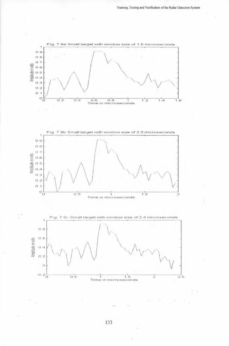
1
0 g-
08
0 .7
Training, Testing and Verification of the Radar Detection System
F i g . 7 9a S mall ta r get vvith vv1ndovv s 1ze o f 1 6 mi c r oseconds
\ \/'
'\ ~ 0 5-
g. 0 4 "'' 1\ '- •. ' \ . ". -._ I v\ r ·
"../ \ ~~; j 0o~----~o~2~----~o~4~----o~6~-----o~8~------1~------1~. 2~-----1~.~4------_J1 6
JtJ
1
09
08
07
~ 0 6 s ~ 0 5 .-E =- 0 4 ~
T ime in microseco n d s
Fig 7 9b S mal l t arget vvi tl, vvi n d o vv s ize of 2 0 mi c r oseconds
I
l
, ;\ I \
\ \,/·· ...
\ \
\ i• • I
03
02
0 1
r··. ,· \} \ / .\ / \\ I
\I \ J 1/ '•./
· .. I\.--\ , . / \1 \.- \ /'\ /\ '\I •!
l
JtJ ~ s (D
-c:> .a ·;:::;_ E
-<C
\,:/ 0o~----~------~o~5~-------------1~-------------1~5~------------~2
0 8
0 6
04
02
0
T1me 1n m1 c r oseconds
F1 g 7 9c S 1,all t arget vvitl, vv1ndovv s ize o f 2 4 mi c r oseconds
/\ \ •'· \ ,..,
............. 1. \, I I I I) \-
( I
I I I
/\ I
\j I I
\
\ I \1
\ \. ' ·,
\, .~ ' J ~ . , _..... • .....
..._\/ . \/ \/ \ I/'.
1/ '\ \/
-o 2o~----------o~5=-----------~1------------1~. 5=-----------~2----------~2~5
T1 me 1 n m1 c r oseconds
133

41 "C ::J ~
Training. Testing and Yerilication oflhe Radar Detection System
Ft g . 7 .9d Small target vvith vvi ndovv size of 2 .8 rni croseconds 1
-O 2o~----=o-'-:s:::-----~1----1:-'-:s=-----2=------::2:-'"_-=s---~3
Time in m 1croseco nds
Fig.7.10 Spread w it h differentwindow size (smal l target)
0 . 8
0 . 6
a. E 0 .4 111 41 >
:0:: 0 . 2 111
Cii ... 0
1 . 6 us 2 . 0 us 2.4 us 2 . 8 us .L
o m _amp 0 .5733 0 . 5022 0 .4547 0 .4308
•m_per 0 . 224 0 . 2 1 5 0 . 1 96 0 . 1877 -oam p_ dev 0 . 1778 0 . 1541 0.1461 0 . 1548
oper_ dev 0 . 2 1 5 0 . 2064 0 . 1882 0 . 1802
• max_per 0 .4 0 .4 0 .4 0.4
om _ amp •m _pe r oam p_dev op er_dev •m ax_per
134

Training, Testing and Verification of the Radar Detection System
Fig.7 .11 a Performance of training with learning rate=0.001, SSE=3.7596 70.-------~------~------~------~----~
60 ~~-·-----------..... --\,
'--50
0 ..__ ..__ w u 40 (]) ..__ ('iJ ::::J
~30 I
E ::::J
(f) 20
10
\
\ \ \
'"'-. ~·------~------
0 ~------~------~------~------~------~ 0 50 100 150 200 250
Epoct1
Fig.7 .11 b Performance of training with learning rate=0 .005, SSE=3.7606 70~------~------~------~------~----~
/\ I I I 60 ,/ \_ .... -,
~---··-·-~..,\
'--0 '-'--w
50
u 40 (]) '--('i) ::::J
~30 I
E ::::J
(f) 20
10
\
\
\ '\
'·--·------~---------OL-------~------~------~------~------~
0 50 100 150 200 250 Epoch
135

Training, Testing Wld Verification of the Radar Detection System
Fig.7 .11 c Performance of training wi th learning rate=0.01, SSE=3.7845 80.-------.------.-------.------~-------.
f\ 10 I \
60j ~ 0 \ tb 50 \
\ \"
20
10 ........ ----~----- ~---------1
o~---~---~---~---~---~ 0 50 100 150 200 250
Epoch
Fig.7 11 d Performance of training wi th learning rate=0.05, SSE=3.6720
70h.
I ,.-\ 60 I/ \p.
"--0 "-"--w
50
u 40 Q) "--m ::J
&30 E ::J
(f) 20
10
I V\
' \\
\ \ \.
\ \
\,_ ... , ..
"'----------·-·---OL_ ___ L_ ___ L_ _____ ~------~----~
0 50 100 150 200 250 Epoch
136
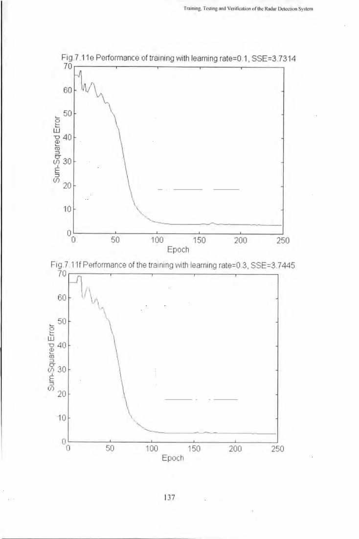
Training. Testmg and Veri fication or the Radar Detection S)s tem
Fig.7 .11 e Performance of training with learning rate=0 .1, SSE=3.7314
70H. 60 1)1~
I '-- 50 \
i40 \ ::J
&30 E ::J
(J) 20
10 \ "--, __
--~----~-----------------0~------L-------L-------~------~----~ 0 50 100 150 200 250
Epoch
Fig.7 .11f Performance of the training with learning rate=0.3, SSE=3.7445 70.-------.-------.-------~------~------.
'--0 '-'--w
60
50
-o 40 Q) '-m ::J
& 30 E ::J
(J) 20
10
](\ [ I I . '•.1\
'·,\
\\
\ I
\ I
\ \
·- ----- ------
o ~------~------~-------L------~--------0 50 1 00 150 200 250
Epoch
137

Training. Testing 1md Verification of the Radar Detection System
Fig .7.12a Performance of training wi th momentum=0.1, SSE=7 .8479 70.-------.-------.-------~------~------.
~l 60 l. .. 1
'-0 ''-w
50
u 40 Q) '-(U ::J
&30 E ::J
(/) 20
10
\ \rj
~ '\ 'l ~_r\
0~------~------~--------~------~------~ 0 50 100 150 200 250
Epocl1
Fig 7 12b Performance of training with momentum=0.5, SSE=4 .9738 70~------~------~------~------~------~ ,,
60 \ \\
\ '- 50 0 ''-w u 40 Q) '-(U ::J
1~\ \
&30 E
I
\ \.
\ \ ,_,
"'-·, --...... _. -------
::J
(/) 20
10 -~--
-----------·-~---
0~------~------~--------~------~------_j 0 50 100 150 200 250
Epocl1
138
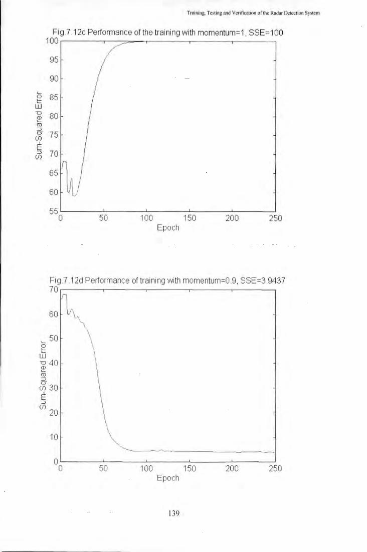
Training, Tesling and Verificalion oflhc Radar Deleclion Syslern
Fig .7 .12c Performance of the training wi th momentum=1 , SSE=1 00 100.------.---=-=-~-------.------~------. .r·-
/'
I 95
90 i I I
>-0 85 >->-w u 80 Q) >-(U :::J IT 75 (f)
I
E :::J 70 (f)
65
1u 60
55 0 50 100 150 200 250
Epoch
Fig.7 .12d Performance of training with momentum=0.9, SSE=3.9437 70~------.-----~------~------~-------,
l 60 V\ ..
\ >- 50
\ \
0 I >- ' >- \ w
I
u 40 I
(j) l >-
\ (U :::J I (l3o \ I
E I :::J \
(f) 20
\ 10
\ \
\
' ·· .. , "- . ..-... ____
0 0 50 100 150 200 250
Epoch
139

Training., Testing and Verification or the Radar Detection System
Fig.7 .12e Performance of training with momentum=0.98, SSE=4 .5261 80~------~------~------~------~----~
·I\ 10 I \ 60 ,v ~~ n
e v lJ \ w 50
~ I }40 ~\f\ E: 30 \
0) vv\. 20 \./\
\F\ '----~\
'··"'"\._. '·----..
...,...'-··-..._ ------10
0~------~------~------~------~----~ 0 50 100 150 200 250
Epocl1
Fig .7 .'l2f Performance of trami ng wi tll momentum=0.95 , SSE=3 .6789 70~------~------~------.-------.-------.
r1 /\ 60 \) \'\
'--0 '-'--w
50
u 40 <D '-c:u =:!
~ 30 I
E =:!
({) 20
10
\ \ \ \
I
\
\ \ \ .,_
''-"'---------------------------
o~------~------~------~------~----~ 0 50 100 150 200 250
Epoch
140

Training, Testing and Verification of the Radar Detection System
To define the topology of the network, a series of tests were performed using different
combinations. These included networks with none, one and two hidden layers, the results with
250 iterations are shown in fi gures 7.13a to 7.13f, which show the initial response of the
network under different topologies. Table 7. 1 shows their sum-squared errors after 30,000
iterations.
Table 7.1 Training errors of the network after 30,000 iterations
Topology
No hidden layer
One hidden layer wi th one neuron
One hidden layer with two neurons
One hidden layer wi th tlu·ee neurons
Two hidden layers with one neurons
Two hidden layers \ ith two neurons
Sum Squared Error
3.0180
3.0231
3.0007
3.0497
3.4937
3.4942
Higher training errors were obtained when the network had none or two hjdden layers. The
optimum performance with least training error was found when the network had a single hidden
layer wi th two neurons and this was chosen for the implementation.
7.4.2 Application of the training algorithm
The developed network with 5 inputs, I hidden layer (with two neurons) and I output layer was
trained with the 250 sets of data. During each epoch, the five parameters of statistical
characterisation were presented to the input layers of the network. For each set of parameters,
the enor was calculated by comparing the network output with the desired output. When the
141

Training, Testing and Verification of the Radar Detection System
entire training set, i.e. 250 sets of input data, had been presented to the network, the error was
summed to update the values of the weights.
In the training algorithm, the training process was terminated by one of two criteria. The first
was to identi fy a maximum error value to ensure that the network would perform to an
acceptable level. However, as the error value might not be reduced to the specified limit wi th the
data available, then under this condition alone training may never be terminated. So, in addition
to this rule, an upper limit was placed on the number of training epochs. The training will then
stop when this maximum specified number is reached. Under this condition, the training time
can be estimated but the performance of the network cannot be guaranteed. In this
implementation, the maximum en or of 0.05 was used as the limit for the training, and it took 3
million training epochs to reduce the error to this value. The first and the last 300,000 iterations
are shown in figures 7. 14a and 7.14b. Training was terminated on the perfonnance rule, when
the etTOr reduced to 0.05.
142

Training, Testing and Verification of the Radar Detection System
Fig. 7.13a Network wi th a single layer, SSE=4 .009 70~------~------~------~------~----~
'- 50 0 ''-w -o 40 (J) '-(U :::J
&30 E :::J
()) 20
'10
0~------~------~-------L------~------~ 0 50 100 150 200 250
Epoch
Fig.7.13b Network wi th one neuron in l1i dden layer, SSE=4 .0675 70~------~------~------~------~----~
/11
60 tft _,- ·'. - -~------·-----.
'-0 ''-w
50
-o 40 (J) '-(U :::J
& 30 E :::J
()) 20
10
'· \
\ I
1\
\
"'----------------- ~--------0~------~------~-------L------~------~
250 0 50 100 150 200 Epoch
143
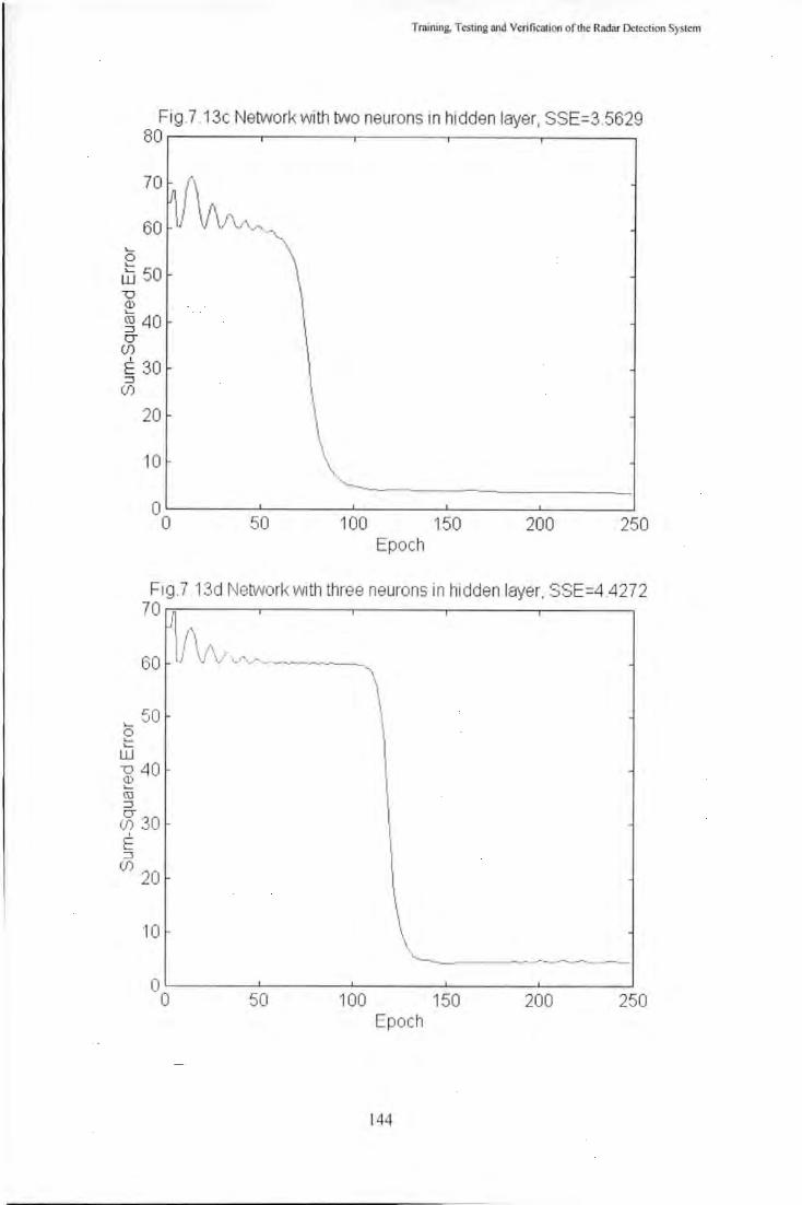
Training, Testing and Verification of the Radar Detection System
Fig.7 .13c Network with two neurons in hidden layer. SSE=3.5629 80~----~~----~------~------~-------,
..... 0 ..... w 50
20
10
\ \ \ \
\~ .....
~------·------~-----------O L-------~------~------~------~----~
0 50 100 150 200 250 Epoch
F1g.7.13cl 1\Jetworl<with three neurons in hidden layer. SSE=4 .4272 70 ~------.-------.-------.-------,-------,
60 V\/\; vv -.--~---\, ..... 50
l40 \11
& 30 I
E :::l
(j) 20
10
0L-------~------~------~------~----~ 0 50 100 150 200 250
Epoch
144

Training, Testing and Veri fication of the Radar Detection System
Fig.7 .13e Network with 2 hidden layers, each with 2 neurons, SSE=4.4288 70.------,.------.-------.-------.-------,
~,
60 \(\/\AJV-.-..--~-----.. ~\
'- 50 0 ''-w D 40 Q) '-(.U :::J
&30 E: :::J
(f) 20
10
0~------~------~--------~------~------~ 0 50 100 150 200 250
Epoch
Fig.7 13f Network with 2 1lidden layers, each with 1 neuron, SSE=4 .0626 70~------~------~------~------~------,
[p,
60 \/\./ ,_F'v··,r..---~~-·----,
'-0 ''-w
50
D 40 Q) '-(.U :::J
& 30 E: :::J
(f) 20
10
\ '\
0~------~------~--------~------~------~ 0 50 100 150 200 250
Epoch
145

Training, Testing and Verification of tile Radar Detection System
Fig .7.14a 2-Layer Backpropagation with Adaptive LR & Momentum, first 300,000 run: 70.------,------.------.------.------.------.
60
'- 50 0 ''-w u 40 (]) '-(IJ :::::1
&30 I
E :::::1
(j) 20
10
0 L~~~=====c==~~======~==~~======~==~d 0 0.5 1 1.5
Epoch 2 2.5
Fig.7 .14b 2-Layer Bacl<propagation wi t11 Adaptive LR & Momentum, last 300,000 runs 0.06 r--------.-------.-------.------.--------.------
'-0 ''-
0.058
w 0.056 u (]) '-(IJ :::::1 er
(j) E: 0.054 :::::1
(j)
0.052
0.05 t.__ ____ __._ ______ ..__ ____ ___J_ ____ -=== 0 2 4 6 8
Epoch
146
10
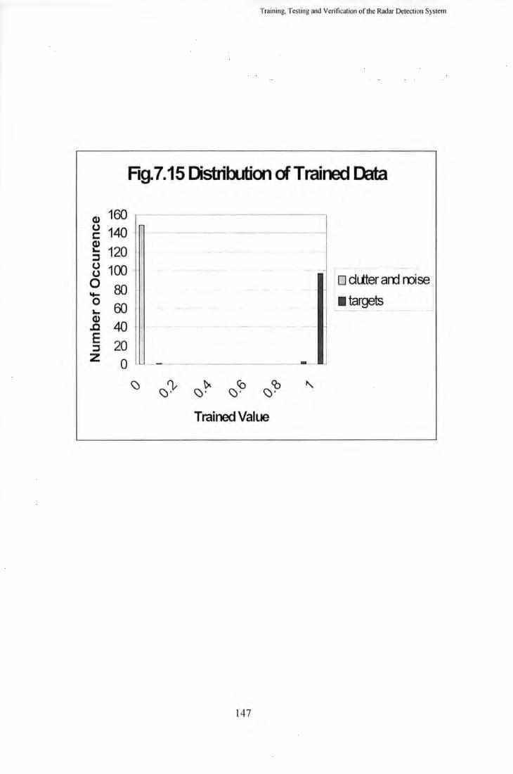
Training, Testing and Verification of the Radar Detection System
Fig. 7.15 Distribution cl Trained Data
Q) 160 ~·- -· -~-~~·--·~ ----0 140 t: - - --- -Q)
120 ... ::I
~ 100 -
0 80 1
D dLtter ard roise '+-0
60 • targets I ... Cl)
40 .c E 20 ::I z 0 -
\:) \)ry \:)~ \:)'<? \:)'?J ~
Trained Value
147

Training. Testing and Verification oftJ~c ~adar Detection System
7.4.3 Testing the 'frained Network
When the training process was terminated, it was necessary to assess the performance of the
trained network with the final values of the weights. Figures 7.14a and 7.14b show the plot of
en·ors against the number of epochs. The rate of change of error reduces as the number of
training cycles increase. Figure 7.15 shows the final result after the training exercises. The
majority of the targets have a value of one while majority of the noise has a value of zero. There
is no overlap between these two values and discrimination can thus be achieved.
A testing process is necessary to verify that the neural network is able to identify targets from
data that was not used in the training exercise. The process was undertaken by using 40 fwther
samples of data with different signal to noise ratio and noise background. Each data set consisted
of a window of 50 samples and the five statistical characterization parameters were extracted
from these data and input to the trained network. The value at the output determined when the
data is a target or noise. Figures 7.16a to 7.16cl show targets with signal to noise ratio of 3. 7ciB,
12.6 dB, 6,6dB and I OdB respectively. Figures 7.17a to 7.17cl shows part of the sampled noise
used for the testing. The testing results are shown in fig. 7.18, where it can be seen that all the
noise samples have an output value of 0 while the targets have an output value ranging from
0. 76 to I. No overlap of the output for targets and noise occurs. Fig. 19 shows the distribution of
signal to noise ratio for targets used in the testing, which ranges from 1.45dB to 24.5dB
148
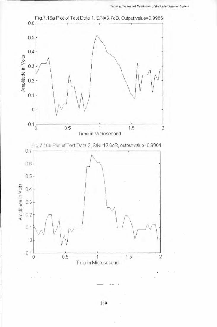
Training, Testing and Verification of the Radar Detection System
Fig.7 .16a Plot of Test Data 1, S/N=3 .7dB, Output value=0.9986 0.6 ,..-------.,--------.-----.-------,
0.5 (\\\ 0.4
I \ ·..,_
(f) "'-,, ±:
,----!\ \ 0 > 0.3 \ ~. c / \
\ \!If Q)
' \ ~c, "0 :::1
-~ 0 2 0. .
E \ j V I <{ 1 I 0.1 \ ~ ) \A I
0 I I \l I 1,/ V
-0.1 L---------'--------'------'-----__..J
0 0.5 1 1.5 2 Time in Microsecond
Fig. 7 .16b Plot ofT est Data 2, S/N= 12 .6dB, output value=O .9964 0.7 ..------,--------.-----.-------,
06
0.5 (f) ......
0.4 0 > c Q) 0.3 "0 :::1 ......
Eo. 0 2 /l
<{ . { \ ' 0.1 \ I' / /I (\~
v\ . \'' !' 0 /\
-0 .1 L__ ___ _.L ____ _.i_ _ ___ __J_ _ __ __..J
0 0.5 1 1.5 2 Time in Microsecond
149
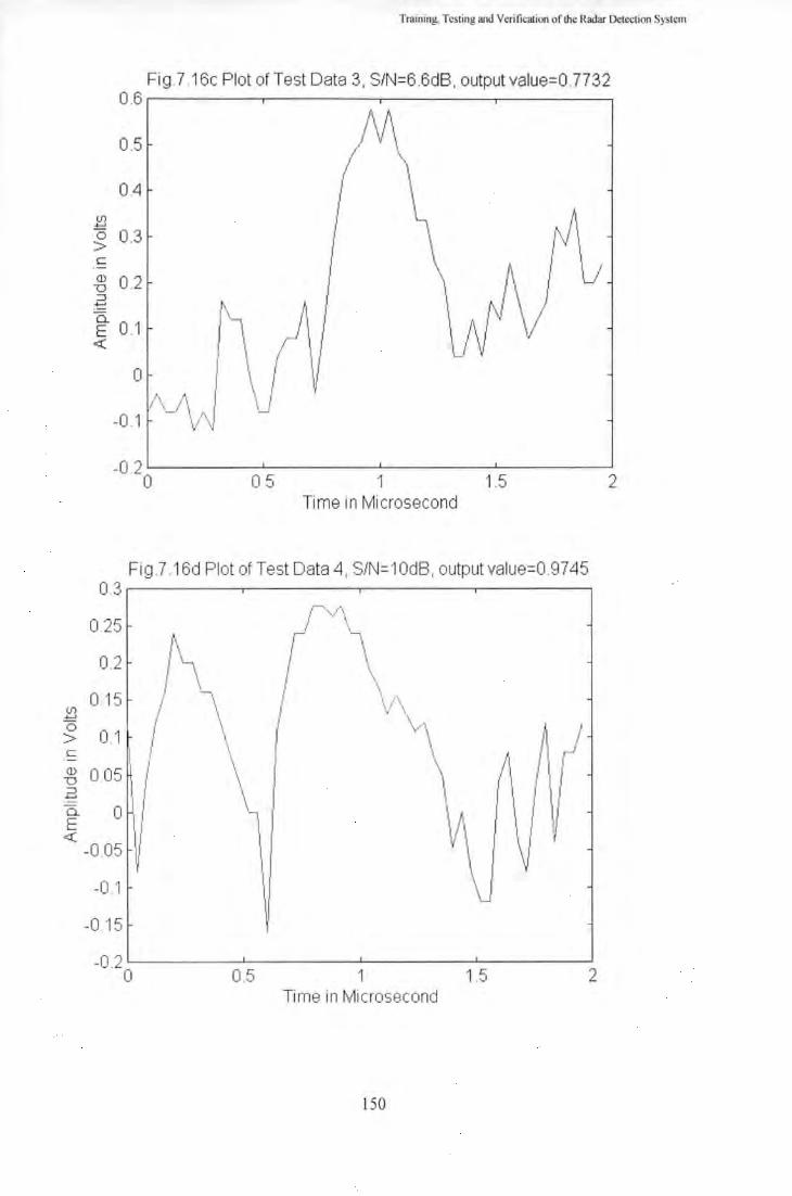
(f) ....... 0 > c Q)
D ::J ....... Q.
E <
Training, Testing and Verification of !he Radar Detection System
Fig .7 .16c Plot of Test Data 3, S/N=6.6dB, output value=0.7732 0.6 r------.,---------r-----.---------,
0.5
0.4 (f)
±::! g 0.3 c
-gj 0.2 ::J .......
-0.2 t.___ ___ __.__ ___ ------1. ____ __.__ ___ ___,
0 0.5 1 1.5 2 Time in Microsecond
Fi g.7 .16d Plot of Test Data 4, S/N=1 OdB, output value=0.9745 0.3
/'v'\ 0.25 .. \
h r ' I I
0.2
I'··~ I \. 015 I ,
/ \ I I .' \
I V ' \ 0.1 I \ I 'v~
\ I I I, I
\ 0.05 I
I
l I
I \ I I 0
·~ I I -0 .05
1/ \J -0 .1
~ I
-0 15
-0.2 0 0.5 1 1.5 2
Time in Microsecond
!50
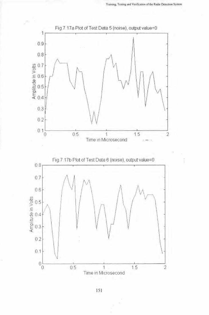
Training, Tes ting and Verification oflhe Radar Detection System
Fi g.7 .17a Plot of Test Data 5 (noise), output value=O 1
0.9
0.8 ,-/'1 I' ~ 0.7 ·~ 0 ; \1\ >
.~ 0.6 (I) D
I \ .~ 0.5 0.. \
~ '\ E ~ 0.4
\ I 0.3 \ ~ '
I
0.2 /V 0.1
0 0.5 1 '1.5 2 Time in Microsecond
Fig.7 .17b Plot of Test Data 6 (noise) , output value=O 0.8
0.7 i\ 1 { I 1\./\ l \ 1
11 /I / \.I I 0.6 I
\ l \ / \ /\ I •
I / I
I •/ I I / \,...---...
({)
I I f \
+-' I I 1 / \ g 0.5 I
,./\\.
I \ /l\ I I,
', I c i '
I 11
~ 04 / I
I I \ I \ I
\ ::J
V \( +-'
IV 0.. I E 0.3 ~
0.2 V \ 0 1 \ 1\
\
0 0 05 1 1.5 2
Time in Microsecond
151

Training, Testing and Verification of the Radar Detection System
Fig. 7.17 c Plot of T est Data 7 (noise), output value=O 0.9 .-----.---------.----------,------,
0.8
0.3
1\ I I
~I( I \ \)
1\ r 11\
I \\ r/\ I /\
I \ 1 \ I t V V
V I/ 0.2 '---'---'-------'--- ----'---------'
0 0.5 1 1.5 2 Time in Microsecond
152

Q) (,) r::::: Q) ... ... ::s (,) (,) 0 .... 0 ... Q) .c E ::s r:::::
Q) 0 c: Q) ... ... :;, 0 0 0 .... 0 ... Q) .0 E :;, z
Training, Testing and Verification ofU1c Radar Detection System
Fig.7.18 Output values for target and noise
25
20
15
10
5
0 C)
4.5 4
3.5 3
2.5 2
1.5
0.5 0
11 li
I _I I I
Output values of the network
Fig. 7.19. Distribution of SIN Ratio
I onoise •target I
~ ~ ~ 0 0 ~ 0 1.{) 1.{) 1.{) 0 1.{) 1.{) 1.{) 0 1.{) 1.{) m
N r--: N N N L.. ,...._ N 0 N ~
SIN Ratio in dB
0 Frequency
153

Training, Testing and Verification of the Radar Detection System
7.5 Investigation of applying the network to a trace of radar of return
The network has been developed to identify whether the window (with 50 samples) is a target or
noise. It has already been shown that there is large discrimination at the output of the network
between target and noise. The next step was to enhance the network to perform the
discrimination in a trace of radar return, which contained more than 50 samples of data. Fig.20a
shows a trace of 100 samples ( 4 microseconds) of radar returns with a target present. To detect
the target in this trace, the 50 sample (2 microseconds) window has to be shifted in time from 0
to 4 microseconds. At first, the window was shifted by I sample each time and the
COITesponding output of the network was recorded, Fig. 20b shows the result. The output has a
result of 1 when the window stru1s from 7'11 sample and this output is maintained until the
window exceeds 85th sample. The output is zero for the rest of the trace. If the window is set to
act as a filter that allows only the samples contained in windows which have an output of one to
pass tlU"ough the detection system, then the resulting output is shown in fig.20c. The detection
system employing this approach would have the fo llowing drawbacks.
I . The process will take 52 cycles of calculating the statistical characterization and
obtaining output from the network.
2. Part of the noise in the vicinity of the target is also accepted by the detection system as
shown in fi g 20c.
To overcome these problems, the number of overlapping cells between each window has to be
reduced. However, the smaller the number of the overlapping cells, the less information is fed to
the detection system. If the number of overlapping cells is made too small. there will be high
chance that a target is missed, in particular the smaller targets that are contained within just a
few samples. In the example of fig.20a, the target would not be detected if the overlap between
windows is less than I 0 samples. By testing the detection system with different amounts of
154

Training, Testing and Vcritication of the Radar Detection System
overlap, it was found that an overlap of around 20 samples gave reasonable results for this
particular target. With this value, only 2 computer cycles were required to obtain the final result
that is shown in fig. 7.20d. The overlap of 20 samples was tested with targets of different sizes
and the result was found capable of discrimination in all cases, on each occasion the target could
be detected with only two computations. The result of using this overlap in the detection a large
target is shown in fi gures 7.20e and 7.20f.
The detection system with this configuration was then applied to a longer trace as shown in
figure 7.21 a. The following methods were used to ensure that the target was correctly identified
from the trace to evaluate the performance of the detection system.
I. The potential targets were confim1ed by checking against the radar display. The gain,
rain clutter and sea cluner controls were adjusted to obtain the optimtm1 settings.
2. If the targets did not appear on the radar display, successful scans of the radar sweeps
were checked to ensure that the target appeared in the radar trace for more than one scan.
3. It the target was in close range, visual confirmation by means of binoculars was used.
4. The radar trace was carefully examined to observe any signs of targets.
As found during the testing stage, there were occasions when the output of the network for some
targets had a value less than I but larger than 0.76. To cater for these types of target, the
detection system was set to accept signals with an output value of 0.7 or more. This would still
allow sufficient discrimination from the noise as described in the early sections. The signal that
is retained after passing through the detection system is shown in fig. 7.21 b and all targets are
detected correctly. For comparison purposes, the same trace was applied to a detection system
using TM-CF AR. which has the best quality of thresholds as indicated in Chapter 2. Again, the
!55

Training, Testing and Verification of the Radar Detection System
comparison was based on the assumption that no false alam1 would occur. The result is shown in
fig. 7.2 1 c. The TM-CFAR detection algori thm uses only the amplitude information and it is
unable to identify weak targets that are embedded in the noise. If the threshold were lowered for
better probability of detection, then it would accept strong noise and clutters and an excessive
false alarm rate would occur. Pmt of these unwanted signals can be removed by scan to scan
correlation and sweep to sweep correlation. However, under such circumstances the existence of
a target can only be confirmed after a few scans and the worst case is that such algorithms
cannot reject correlated noise and clutters. It is important to note that the developed detection
system can detect weak targets as well as retain the shape of the waveform for further use in
pattern recognition processes.
Ten traces of live radar returns, which were not used in the training process, were used to test the
developed system. Weak targets with low signal to noise ratio were added to the clutter edges in
some traces. The results showed that the system was able to discriminate weak echoes from
strong clutters by using the five statistical parameters, i.e. mean amplitude, mean amplitude
deviation, mean pulse width, mean pulse width deviation and ma'<imum pulse width. The results
of some of the tests are shown in figures 7.22 and 7.23 where the perfotmance ofthe TM-CFAR
detection for these two traces is also shown for comparison. In fig. 7.22a, the retum signal
consists or rain clutters with a weak target at the clutter edge. The signal to noise ratio at the
edge of the rai n clutter is --4.97d8. Fig. 7.22b shows that all targets are detected by the neural
network. The TM-CFAR system (fi g. 7.22c) is not able to adapt to the clutter edge and detect
the weak echo. In f1g. 7 .23a, targets are detected from a radar trace with strong sea clutters. The
signal to noise ratio of the weakest target is 5.19d8. Again, the result from TM-CF AR in such
clutter environment is not satisfactory (fig. 7.23c).
156

Training, Testing and Verification of the Radar Detection System
Fig.7.20a A Trace of Radar Return wi th 100 Samples 1.---~---,,---~--------~--~----~---.
0.8
~ 0.6 0 > c
-02~--~--~~--~--~----~--~----~--~
0 0.5 1 1.5 2 2.5 3 3.5 4 Time in Mi crosecond
Fig.720b Output of the Networldor the trace in Fig.7 .20a 1
0.9
0.8
~ 0.7 0
~ I Q) 0.6
z Q)
£0.5 ..._ 0
::5 0 .4 0.. .._. ::::J
0 0 3
0.2
0.1
0 0 0.5 1 1.5 2 2.5 3 3.5 4
Time in Microsecond
157

Training. Testing and Verification of the Radar Detection System
Fig.7 .20c Output of the detection system with a shift of one sample 1.---~----~--~--------~--~----~--~
0.8 \ ..... \
(f) 0.6 \ ....... 0
I > c ·-Q) 0.4 -o l ::::J ....... o._ l{l f1 E
11 \ I <( 0.2
1 ~vi\ d /\ v-" ~vn( 1 I \1 \1 J 0
__ j I h
_/ I I
-0 .2 0 0.5 1 1.5 2 2.5 3 3.5 4
Time in Mi crosecond
F1g 7 .20d Output of the detection system with an overlapping of 20 samples 09~--~--~~--~---.----~--~----~--~
0.8 ~I
1\ 07 I 06 \ (f)
I ....... 0
0.5 > I c ·- I Q) 0.4 -o
l\1 ::::J
l ....... o._ 0 3 E <( I
\P 02
(V\n/) 0 1 \ ''~'In .- I I 0 / I
-0 1 0 0.5 1 1.5 2 2.5 3 3.5 4
Time in Microsecond
158

Training, Testing and Verification of the Radar Detection System
Fig .7 .20e A Trace of Radar Return with 100 Samples (large target) 1.8.----.----~--~----.----,,----.----.----.
1.6 l I
1.4
(f) 1.2
.±= 0
1 > c ·-Q) 0.8 u :::J .......
E- o.6
c 04 I . J
\ h /1 0.2 I j I' ;'\ \ q ( \
\ /., '\1 \ \ ,_ ·~ Af\\ r/\;..;1 ~~ o --v V \fvl v\ J \J!\·J
-0 .2 L-----'-----....L..._-----L. ____ _..__ __ ----..J.___ __ __,_ ____ .....______._____,
0 0.5 1 1.5 2 2.5 3 3.5 4 Time in Mi crosecond
Fig.7.20f0utput of the detecti on system witll an overlapping of 20 samples (large target) 1 .8 .--------.----.-----r--------.----.-----r------,---
1.6
1 4
1.2
g 1 c
Q) o.s I i o.6 I
~ o4 I i
0.2 I ; · AJ \~. /l. ~"'~ ~~ 1 1 \/
0 \ I I;' 1\/, I - I I 11/\
' I . I I -0.2 ._ _ __._ ____ _..__ ___ .__ __ __._ ____ _,__ ____ .___ __ __,_ __ ____,
0 0.5 1 1.5 2 2.5 3 3.5 4 Time in Microsecond
159

Traming, Testing and Verification of the Radar Detection System
Fig. 7.21 a A Radar trace with 2000 Samples 1 .----.-----.----.-----.-----.----.--.--.--~
0.8
0.6 (J')
.±:::! 0 > c 0.4 Q)
"D ::::J
~ 0.2 E <(
0
-0 .2
7
4 6
1
2
5
-0 .4 L.__ _ __.._ __ _,___ _ __._ __ _,___ _ __._ __ __.__ _ __.__----J
(J') .±:::! 0 > c ·-Q)
"D ::::J ....., 0... E <(
0 1 0 20 30 40 50 60 70
1
0.8
06
0.4
0.2
0
-0 .2 0
1
2
~
10
Time in l'v1icrosecond
Fig.7 .2'1 b Output of the detection system
3 7
4 6
5
1-
20 30 40 50 60 70 Time in Microsecond
160
80
80

Training. Testing and Verification or the Radar Detection System
Fig.7 .21c Sea Target Signal witll TM-CFAR Threshold , T1=40,T2=40) 1~--~--~~--~----~----~--~~--~--~
0.8
0.6
0 2 ~ 04 Q)
u :::l
-~ 0.2 E <(
0
-0 .2
-0.4 L-----1---'-----l..------.Jl_..__-l..-_-----l. __ _.._ _ __,
0 1 0 20 30 40 50 60 70 80 Time in microseconds
Fig.7 .21 d Signals accepted by TM-CFAR 0.2~--~----~--~----~----~--~----~--~
0.18
0.16
0 14
~ 0 12 c:
.gs 0.1 :::l .......
E-0.08 <(
0 06
0.04
0 02
3 7
o ~--~--~~--~----~----~--~~--~--~ 0 10 20 30 40 50 60 70 80
Time in microseconds
161

(f)
== 0 > c
·-Q)
D ::J ....... 0. E <(
1.4
1 2
'1
08
0.6
0.4
0.2
0
-0 2
-0 4 0
3
l 2
4
I
'-----
10
Training, Testing and Verification of the Radar Detection System
5 9
10
7 11 8
6
f- -
20 30 40 50 60 70 80 Time in Microsecond
162

(f) .......
Training, Testing and Verification of the Radar Detection System
Fig .7 .22c Sea Target Signal wi th TM-CFAR Threshold, T1 =40,T2=40) 1 . 6 .----.----.----.----.----.----.----.--~
1.4 3
1.2
0
-0 .2
-04 ~--~----~--~----~--~----~--~--~
1
0 9
0.8
0 .7
0 10
3
20 30 40 50 60 70 80 Time in microseconds
Fig.7 .22d Signals accepted by TM-CFAR
5
9 10 ~ 0 .6 c
.g 0.5 ::J .......
E-0.4 ~
0.3
0 2
0.1
0 0
2
4
10 20
11 7
8
l 30 40 50 60 70 80
Time in microseconds
163

Training, Testing and Verification of the Radar Detection System
Fig.7 .23a Radar trace with sea clutters 1.2
4
1 2
0.8 3
(J) ±:=
0.6 0 > c 1 ·-
7 5
6 Q)
0.4 "0 ::J ....... 0. E 0.2 <(
0
-0 .2
-0 .4 0 10 20 30 40 50 60 70 80
Time in Microsecond
Fig.7 .23b Output of the detection system 1.2
4
1 2
0.8 3
(J) ....... 0.6 0
> c
5 7
1 6 ·-Q)
0.4 "0 ::J ....... 0. E 0.2 <(
0 L r-----'
' -0.2
-0 .4 0 20 40 60 80
Time in Microsecond
164

Training, Testing and Verification of the Radar Detection System
Fig.7.23c Sea Target Signal wi th TM-CFAR Threshold, T1=40,T2=40) 1.2.----.----.. ---.----.----.----.----.--~
1
0.8
(f) .._. 0.6 0
> c Q)
0.4 '"0 :::J .._. -a. E 0.2 <(
0
-0.2
-0.4 0 10 20 30 40 50 60 70 80
Time in microseconds
Fig.7 .23d Signals accepted by Ttvi-CFAR 0.7
4
0.6
0.5 (f)
.±:::1 0
~ 04 Q)
'"0 :::J
-~ 0 3 a. E <(
0.2 2
0.1
0 0 10 20 30 40 50 60 70 80
Time in microseconds
165

Training, Testing and Verification ofth<; Radar Detection System
7.6 Investigation of parameters required for target classification
Radar systems transfonn complex infonnation from the targets into a one-dimensional
wavefom1, which only presents the amplitude infonnation of the target at different times. The
earlier sections show how the five statistical parameters (extracted from these wavefonns) may
be used in the detection of marine targets. To develop the study further, it would be necessary to
see if the extracted features can also be used in the target classification process. In general cases,
radar observers would first classify the targets into two types, i.e. large and small vessels. Large
vessels refer to bulk carriers, warships, tankers, general cargo ships and so on. Small vessels
include pleasure craft, tugboats, fishing boats .... etc. After this preliminary classification, a
follow up detailed classification could be carried out for further pattern recognition to identifY
specific types/groups of targets. In order to reach the second stage, it is critical that the
preliminary classification is efficient and accurate. The objective was to develop the technology
further and investigate the potential for a system that can classify the targets into the two primary
groups, The accuracy of a target recognition system depends on the certainty of their extracted
features. The extracted feature should have the characteristics of the targets only and should not
be affected by other external parameters such as range and the clutter environment. These
features or their regular changing patterns can be observed at different time intervals.
Two groups of vessels. large and small were extracted from the radar traces. These are
distinguished by visual observation of the vessels as well as by manual inspection of the return
signals. l'vlost of the aspects of viewing were from the broad side however, on some occasions
echoes fi·om the front side of the vessels were recorded.
To determine the features required in the target classification process, it is necessary to look at
the discrimination properties of the five parameters for these two classes of vessels. The results
166

Tmining, Testing and Verification ofi.he-Radar D~tcction System
are shown in figures 7.24a to 7.24e. It can be seen that there is less discrimination in the period
parameters than the amplitude parameters and there is noticeable discrimination in the amplitude
deviation. Despite the fact that period parameter will give some indications about frequency
components of the retum wave, the simplified method that has been adopted to date, in order to
reduce the computation time, might not be able to provide the necessary details of the frequency
distribution. As such, the immediate frequency method as described in Chapter 5 can be adopted
in analyzing the target wavefonn in the frequency domain. The immediate frequency of each
target was calculated. The discrimination in the immediate frequency between these two types of
target is plotted in fig. 7.24f and shows that effective discrimination may be achieved with
inclusion of this parameter. Therefore, these two parameters, i.e. the amplitude deviation and the
instant frequency were used to set up the target classification system.
The one-dimensional retum from the same target would vary from sweep to sweep as well as
from scan to scan. It is difficult to specify a definite value about the parameter describing the
class of targets, instead it is really a fuzzy pattern classification process. Figure 7.25a and 7.25b
show the variation of the amplitude parameters and the period parameters between the two types
of targets for 5 consecutive scans. The immediate frequencies and the amplitude deviation of
these two target types vary from scan to scan and their variations are shown in table 7.2.
167

Training. Tc5ting ami Vcrificmion of the Radar Detection System
Table 7.2 Variation of Immediate Frequency and Amplitude Deviation between 5 scans
Scan 1 2 3 4 5
Imme. Freq. (large vessel) 2.6370 2.6762 2.8950 2.7366 2.5336
Amp. Dev. (large vessel ) 0.337S 0.2S39 0.2S 19 0.3224 0.3127
Imme. Freq. (small vessel) 2.0327 1.8309 2.4602 1.8631 1.967S
Amp. Dev. (small vessel) 0.2900 0.6104 0.3S 17 0.4200 0.1772
In view of the variations of the two parameters between scans, a fuzzy approach would be
required to deal with the input data to the classification system. To maintain the performance of
the neural network in the detection system, a neuro-fuzzy technique was used to classify these
two types of targets. This approach has the benefit of handling the two parameters in fuzzy tenns
as well as training a suitable network to achieve the task of classification. The block diagram of
the neuro-fuzzy approach is shown in fig. 7.26.
The input parameters were first fuzzified by means of the membership functions in fig 7.27. The
functions were derived fl·om the statistical distributions of the I 00 samples, i.e. SO samples of
large vessel and SO samples of small vessel. The fuzzified data was then used as input for
training the network with lour input layers, two hidden layers and one output layer.
A similar neural network approach to that adopted in the detection was used to recogmse
specific targets from the radar retums. The network was trained using 100 samples to classify
targets into large vessels (0) and small vessels (I). The output from the neural network system
for the 20 test targets is shown in table 7.3.
168

Training, Testing and Verification of the Radar Detection System
Table 7.3 Testing set for the neural network
TARGETS OUTPUTS FROM THE NEURAL NETWORK
Small (I to 5) 0.5987 0.5468 0.55
Small (6 to I 0)
Large ( I to 5) 0.032 1 0 0 0 0
Large (6 to I 0) 0 0 0 0 0
It can be seen that there is no overlap between the outputs for the tvvo types of targets, and by
using a threshold of 0.5, the network classifies the targets into large and small vessels.
Q) (..) s::::: Q) .... :::l (..) (..)
0 ..... 0 .... Q) .c E :::l s:::::
Fig. 7.24a Discrimination in Mean Amplitude
14
12
10
8
6
4
2
0 <::) <::)~ <::)'} <::)'? <::)~ <::)~ <::)~ <::)'\ <::)'?J <::)?:>
amplitude in volts
-+--small target -a- large target
169

Training, Testing and Verification or the Radar Detection System
Fig.7.24b Discrimination in Amplitude Deviation
20 Cl) 18 (J c: 16 Cl) .... 14 :::J (J 12 (J 0 10 -0 8 .... Cl) 6 .c E 4 :::J
2 c: 0
<;:) " ~<y ~~ ~~ ~~ <;:)'? ~~ <;:)·
amplitude in volts
-small target - large target
Fig.7.24c Discrimination in Mean Period
30 - - -- - - ----l Cl)
25 (J
c: Cl) ....
20 :::J (J (J
0 15 -0 ....
10 Cl) .c E :::J 5 c:
0
0 0.05 0.1 0.15 0.2 0.25 0.3 0.35 0.4 0.45 0.5
period in microseconds
- small target - large target
170

Training, Testing and Verilication of the Radar Detection System
Fig. 7.24d Discrimination in maximum period
25 Q,) (J
20 c:: Q,) '-:I (J 15 (J 0 -0 10 '-Q,) ..c E 5 :I c::
0
period in microseconds
-+-small target - large target
Fig7.24e Discrimination in Period Deviation
30
Q) 25 (J
c:: Q) '-
20 :I (J (J
0 15 -0 '-
10 Q) ..c E ::I 5 c::
0
0 0.05 0.1 0.15 0.2 0.25 0.3 0.35 0.4 0.45 0.5
period in microseconds
-+-small target - large target
171

T raining, Testing and Verification o f the Radar Detection System
Fig.7.24f Discrimination in Instant Frequency
9 ------- ------------------Q) 8 0 s::::: 7 Q)
:; 6 0 0 0
0 4 ... Q) 3 .c E 2 :::J s::::: 1
0 ~ ~ m ~ ~ ~ ~ m ~ ~ ~ ~ m ~ ~ ~ ~
0 • • • • •
~ ~ ~ N N N N N ~ ~ ~ ~ ~ ~ ~ ~ ~
frequency in MHz
--+-small target -- large target
172

Training, Testing and Verification of the Radar Detection System
Fig. 7 .25a Radar Return Sequence of Large Target 1.6 .------,------,-----r------,
1.4
1.2
-0.4 .___ ____ ...___ _____ ._ ___ ____. ____ ___, 0 0.5 1 1.5 2
Time in microseconds
Fig. 7 .25b Radar Return Sequence of a Small Target 1 .2~----~---~.-----~-----.
-0.4 L-------'~-------'--------1.------'
0 0.5 1 1.5 2 Time in microseconds
173
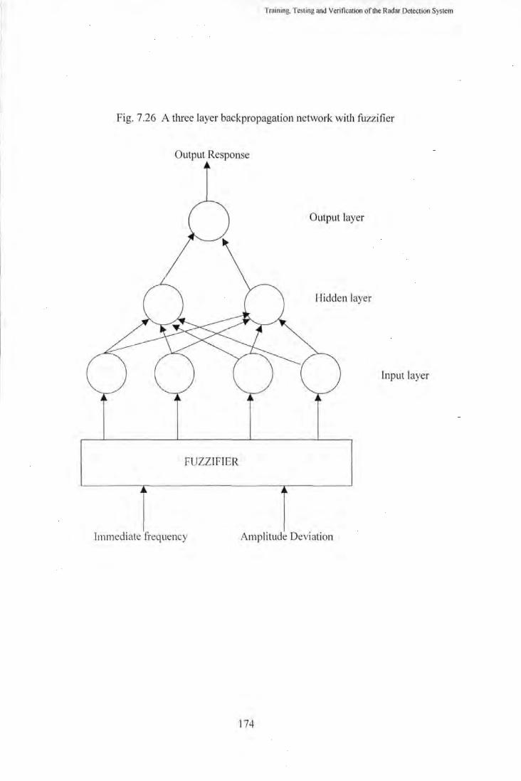
Training, Testing and Veri fication of the Radar Detection System
Fig. 7.26 A three layer backpropagation network with fuzzifier
Output Response
Output layer
Hidden layer
input layer
FUZZIFIER
Immediate frequency Amplitude Deviation
174

Training, Testing and Verification of the Radar Detection System
Fig. 7.27a Membership Function of Amplitude Deviation
0.1 0.2 0.45
Amplitude Deviation in volts
Fig. 7 .27b Membership Function of Immediate Frequency
2.2 2.7 4.7
Immediate Frequency in MHz
175

Trnini11g, Testing and Vcrilication of the Radar Detection System
7. 7 Conclusion
The neural network has been developed and optimised for use with the target detection system
and enhanced to cater for a basic classification capability. Initially, studies were made to define
the network topology as well as formulating the network parameters. The system was trained on
250 waveforms that were extracted from live radar recordings on a system that is located at the
University of Plymouth. The \Vavefom1s consisted of different targets, noise background, sea
clutter and rain clutter. After the training process was completed, the developed system was
tested to assess perfonnance. The performance of the detection system was compared with the
Tl'vl-CFAR system and the result showed that the neural network based system has a much better
capability for detecting targets amongst the variation in noise backgrounds presented. it can
detect the targets correctly and retain the waveform of the retum signals after the detection
process.
The testing waveforms have included a variety of situations which have not been met by the
system during the training process. Out of the 20 radar traces used in the training, two extreme
cases with strong rain clutters and sea clutters were shown. The results of the testing process
showed that the network had learnt to identify targets from clutters under all test situations
presented to it.
There were difficulties in obtaining sufficient samples to build up the database for both training
and testing. As such, a lot of time has been spent in recording the return signals from vessels
passing the harbour, and waiting for oppor1unity to record these under the varying backgrounds
including sea clutters and rain clutters. Despite the fact that there were errors in the network
output alter the training. there were still enough discriminating space between the target and the
clutters for the detection process to give the appropriate response. The same philosophy, with the
176

Training., TeSting and Verification Of the Radar Detection System
addition of a fuzzier to match the uncertainties, was used in perfom1ing target classification, It
proved that the system could classify the targets presented into large and small vessels
effectively. To further recognise the vessels to specific types, e.g. destroyer, cruiser, cargo ship
... etc, more samples would be required to train the neuro-fuzzy identifier. A comprehensive
simulation environment with different models would be desirable to provide the wide variety of
samples that are required for training.
The results from the trials have proved to be encouraging. Simple processing techniques were
able to provide valuable infmmation from the radar signal and fw1her computer methods were
then able to detect the targets based on this infom1ation. The feature extraction process involved
only simple mathematics. The objective was to avoid the use of complicated algorithms that
require significant computation time. This would limit the application of the system in real time
environment where speed of the process is essential. The speed could ftn1her be improved if all
or part of the tasks were to be perfonned under parallel hardware implementation.
The developed system is designed for radar target detection and classification purposes.
However, the same design concept can also be applied to other signal detection process, such as
medical imaging and pattern recognition.
177

Conclusion and funher '''ark
CHAPTERS
CONCLUSIONS AND FURTHER WORK
8.1 Introduction
The aim of this study was to adopt an artificial intelligence approach to the processing
of radar return signals for target detection. The programme of work has involved the
evaluation of artificial intelligence and the use of neural networks in this application.
The research work was divided into a subset of major tasks:
a. Survey of existing detection algorithms;
b. Investigating the feature extraction techniques;
c. Studying the possibilities of employing neural networks in target detection ;
d. Developing software and hardware for acquiring radar signals for use in the
research;
e. Formulating the neural network based detectioi1 system;
f. Considering the extension of these methods for the classification of targets.
Recent research into radar target detection has concentrated on the improvement of
the existing CFAR algorithms. This study has used a new approach in which detection
is based on features extracted from the raw radar data.
This chapter summaries the key findings, draws conclusions from the results of this
investigation and considers the possibilities for future developments.
Conclusiori andifurthcr work
8.2 Approach to the solution of problems in target detection
In the design and evaluation of an intelligent target detection system, the following
related problems have been considered.
8.2.1 Drawback of commonly used detection algorithms
Various current methods for target detection in radar have been discussed in chapter
one. In a marine radar environment, both ground clutter and sea clutter can cause
difficulties in detecting target vessels. These clutters often have sufficient magnitude
to mask targets in a region. Clutter changes dramatically as the radar antenna turns. In
one location of a single scan, clutter returns from a calm sea may be observed which
behave as Rayleigh distributed random variable. In other locations, clutter returns
from coastal waters, where land sea interface is situated, are observed. This clutter
often behaves as a K-distributed random variable and the detection process in the
clutter edge is very unpredictable. Under such a variety of circumstances, a simple
detection method employing threshold techniques alone cannot meet the challenge
and excessive false alarms or failed detections will be encountered. A comprehensive
range of variations on the CF AR detection algorithm has been discussed. Each these
aims to tackle a specific problem in detection, e.g. GO CFAR is appropriate for
improving performance near clutter edges, SO CFAR was developed to detect closely
spaced targets, OS CF AR is considered as a processor to deal with interfering targets.
It is concluded in chapter I that no single CF AR algorithm, where the decision is
made only from the amplitude information of the return echoes, is adequate to solve
problems in a complex detection environment.
179

Conclusion and fun her work
Research into alternative methods of target detection was reviewed. Papers reporting
the success of application of fuzzy logic in signal detection has instigated the
application of artificial intelligence in the area of target detection in radar. Fuzzy logic
has a distinct advantage over other algorithms in handling information that has a high
degree of uncertainty. The membership functions are assigned to the prior
probabilities, the cost function and the received signal amplitude. Based on a
particular situation and the corresponding statistics of the noise under each
hypothesis, the processing mechanism works with this fuzzy information to determine
the desired threshold. However, the final threshold depends on the shape of
membership functions of the input parameters. It is necessary to ensure that the
assignment of the membership is appropriate to the operating environment of the
radar system. Also, the selection of rules plays an important role in the performance
of the final system. The rules should be formulated to cover all the aspects that the
radar will encounter. As such, it is difficult to achieve the optimum state when a fuzzy
approach is adopted.
8.2.2. Extraction of features from radar signals
The primary limitation of traditional information processing techniques is their static
processing methods which employs only the magnitude of the signals. With recent
development in the processing speed of computers, more information can be handled
in real time. Important information from radar returns, such as spatial components,
amplitude deviations and so on, can be extracted to assist in deciding if a target is
present. Theoretical analysis and experimental results provided in chapter 3 on one
dimensional space of the radar waveforms show that characteristics of radar targets
and clutters are different within a certain degree. Such differences were observed on
JRO

Conclusion and further work
signals recorded from a general purpose marine radar and compared with expected
values from knowledge/data bases to make a decision regarding the presence of a
target. However, it is necessary to identify the amount of information required to
make decision process in target detection efficient, bearing in mind the requirement to
solve the problem in a computer in real time. For the purposes of this investigation, a
number of characteristics of the return signal were identified. Conventional waveform
analysis techniques such as Fourier transform and correlation were evaluated. These
involve complex computational sequences, which did not prove to be practical for real
time processing. Statistical signal characterization involves the division of the
waveform into segments, which are bound by positive and negative extreme
conditions. Eventually, five waveform parameters namely; amplitude mean, amplitude
deviation, period mean, period deviation and maximum period were identi tied as the
pnmary measures appropriate to this application. The use of these measures can
achieve similar objectives to spectral analysis and correlation, but they need
significantly fewer computer operations. Each set of waveform parameters is unique
to a particular waveform. In very complex situations (e.g. heavy clutter), a
redundancy may spread across more than one parameter between target and noise, but
it does not spread across all the five parameters to a degree which is beyond the
computational capabilities in discriminating the features.
8.2.3. Data acquisition of radar signals
The radar equipment used within this investigation is a general purpose marine radar,
which looks out across Plymouth harbour. Ideally, the research required a data
acquisition system that is able to record the radar signal continuously for a number of
scans and incorporate bearing identification in each sweep. Such a recording system
I RI

Conclusion and I runhcr work
was not available on the market during the research period, however it was at the
development stage. This demonstrates the industrial drive towards further digital
methods in the processing of radar return signals and the imminent possibility of
implementation of this research. In order to progress with the original objectives, it
was decided that a simple system should be designed to acquire the radar signals and
transfer the data into a computer for analysis. The system consisted of a digitized
oscilloscope with a maximum sampling frequency of I OOMHz which was able to
record the signal for a number of sweeps, depending on the sampling rate used. The
heading marker was employed as a trigger signal to initiate the recording and any
targets passing the heading marker region could be recorded. As the existing heading
marker of the radar at the University of Plymouth was in a radar blinding sector, a
simple hardware circuit with variable delay was designed and built. This enabled the
heading to be shifted by around I 0 degrees and facilitated the acquisition of returns
from targets over a sector that looked across Plymouth Sound and beyond. The
recording system proved to be satisfactory and was used to record over 300 sweeps
from the radar transceiver to form a database of digital radar return signals. This
included a variety of targets, sea clutter, rain clutter, land clutter and noise. A
substantial amount of time was spent recording these returns, and it was also essential
to maintain visual observation to verify and catalogue targets that were observed
passing the heading marker region.
8.3 The application of neural networks to radar detection
The information fusion techniques using neural network have been discussed in
chapter four. The strategies were based on a multi-layer perceptron network with
backpropagation learning algorithms. The research concentrated on the application of
IR2

ConcluSion and funher work
neural networks to improve the target detection and did not intend to develop new
neural theories or revolutionary learning. Research into applications is a relevant
subject of interest. The topology, structure, training requirements and input
parameters are application dependent and the theory has not yet been developed to
provide a rule base for design. By studying the performance of various topologies, a 3
layer network with 5 inputs and I output was formulated to investigate the use of
neural networks in solving complex detection problems. The five statistical
characteristics were extracted from 250 samples of radar signals. The 250 samples
were chosen to represent a wide variety of signals that would encompass the range of
conditions that a radar system is likely to encounter in a complex port environment.
Test runs were performed to determine the optimum parameters for use in the learning
process, such as learning rates, momentum values and network structures.
The integrated system and the results have been described in Chapter 6 and Chapter 7
respectivdy. The resulting neural detection system was able to identify targets from
samples of radar signals even at low signal to noise ratios. The performance of the
network was found to be similar under both training and testing conditions and the
maximum error of 0.05, chosen in the training process, allowed sufficient margin for
the discrimination between targets and noise. In applying the detection system to the
real time situation, a moving window was shifted along the complete sweep. The
effect on the number of overlapping samples in the window was studied to obtain the
optimum setting. Sweeps containing strong rain clutters and sea clutters were used in
testing the system and the results showed that the network is able to discriminate
targets that are embedded in the clutter edge. For the purpose of comparison, a TM-
IR3
Conclusion and furiher work
CFAR algorithm was tested with ·the same sweeps of radar signals and was unable to
perform satisfactorily under such adverse conditions.
The neural detection system was further extended to include a fuzzifier to investigate
the potential for classification of targets. The inclusioil of fuzzy logic, and with
immediate frequency as an additional input, the process was able to handle the
uncertainties of the parameters between scans/sweeps, The combined neural-fuzzy
system was able to classify the targets into large and small vessels by using only two
parameters, i.e. amplitude deviation and immediate frequency, with satisfactory
·results.
8.4 Contribution of this study to radar detection system
The result of this study is considered to be a break through in the existing technology
of radar detection. The developed technique does not use the conventional CFAR
algorithms to determine the thresholding level of the amplitudes. Instead, important
features from the raw radar videos are extracted to determine the presence of a target.
The features are not limited to the amplitude parameter, information such as
amplitude/period deviation from the mean, mean period and maximum period are also
used in the task of detection. The study introduced the concept of adopting data fusion
in the detection stage of the radar signal processing to combine the extracted features.
Live video was used in training the neural network to facilitate the developed system
to handle the real radar data. The result showed that the system is efficient and is able
to detect targets even when the amplitude is lower than that of clutters and
background noise. The existing detection algorithms only accept the part of waveform
that is above the threshold amplitude. As such, some valuable information in the
IR4
Conclusion and further work
waveform will be lost. With the neural detection system, a large section of the target
waveform was retained after the detection process and this information is available for
use in subsequent processing such as target identification, as well as the tracking
stage. This can further be used to improve the tracking reliability of present radar
systems. The introduction of a neural-fuzzy system has demonstrated that the system
was able to handle fuzzy data and classify the targets into small and large vessels.
This neural-fuzzy approach can form a framework for any future sophisticated radar
target identification processes.
8.5 Future developments
The work produced by this research has established an intelligent target detection
system that can be used as a basis for the development of future detection methods in
radar or other areas, such as recognition of patterns from medical instrumentation. To
implement the developed system in pattern recognition, similar parameters can be
extracted from incoming signals. Provided that redundancies do not appear in all the
five parameters, then an individual database for different types of signals can be
formulated to meet the requirements of the specific application.
To further develop the system, it is suggested that the following improvements and
future research are necessary.
Additional outputs and inputs to the system
The use of more sophisticated data recording system
Using high speed parallel processor
The investigation of alternative intelligent algorithms
The use of additional features in the classification of radar targets
IR5

Conclusion and further work
8.5.1 Additional inputs and outputs to the system
The system has five inputs to the neural networks and these are mean amplitude, mean
amplitude deviation, mean period, mean period deviation and maximum period. The
neural network has only one output that is the weight to determine if a target is
present in the window. The system could be enhanced if the environmental condition
could be used as further inputs. The information on the sea-state or wind speed will
provide the system with information regarding the amount of sea clutter that the radar
is likely to receive. The database can then contain sea clutter signals at different sea
states and this will assist the system to discriminate targets from heavy sea clutters.
Similarly, the precipitation condition will provide important information about the
expected magnitude of the rain clutters.
The system could also be improved by producing outputs that are able to classify the
input waveform into different categories. To achieve this requirement, the system
would require a comprehensive database of different signals, which would in turn
require a sophisticated data recording system. Also, the measurement of simulated
targets in a controlled environment with different models of targets, such as could be
provided in an anechoic chamber, may be necessary. This classification would enable
the radar tracking system to process interesting signal/targets only. This would greatly
reduce the processing time needed by the computer.
8.5.2 The use of sophisticated data recording system
The present recording system employed a digital oscilloscope which is limited to the
size of memory in the equipment and hence can only record a few sweeps of radar
signals at one time. As such, it is necessary to transfer the data between the
IR(i

Conclusion and fLirther·work
oscilloscope and the computer after each recording. This procedure caused difficulty
in building up a long history of radar returns from specific targets. The ideal system
should integrate the digitizer with a computer so that data can be transferred
automatically when the buffer memory is full. llhe recording system should also be
able to identify the bearing of each sweep uniquely so the targets at specific sectors
can be searched quickly; however they would still need to be identified and
catalogued visually. With this type of system, the radar returns from different types of
targets could be recorded at various ranges and an extensive database constructed.
Fw1her training of the neural network with more extensive data would improve the
probability of detecting and identifying individual types of targets. It is understood
that a company based in Russia is designing a digital acquisition system to work with
its radar systems. Unfortunately, there is no indication as to when such recording
system will be available in the market, or of the facilities that will be available to
extract digital data from their dedicated hardware. This is a requirement for the
purposes of further research into methods for integrating this detection system with
the radar tracking processes to enhance the capability of the tracker.
8.5.3 Using high speed parallel processor
The detection system has to extract the features from windows of radar signal
sequentially, then the features have to input to the neural network to decide the output
value. This will take up considerable amount of computational time and induce delays
in the detection system. For practical implementation, the delay can be improved by
employing parallel high speed signal processing chips, e.g. TMS 320 family, to
perform feature extraction of the radar returns. The duty of inference can then be
performed by a fast speed PC, e.g. with a P3 family CPU. This arrangement will
IR7

ConClusion and further work
enable better efficiency in the real time implementation of the target detection and
recognition process.
8.5.4 The implementation of alternative artificial intelligence methods
The detection algorithms that have been studied are CF AR, fuzzy logic and neural
network. The CF AR algorithms could not achieve the detection capability in adverse
conditions due to their decision being based on amplitude information only. The fuzzy
approach has many successful applications in engineering fields, but it requires the
definition of a reliable rule base. In the area of target detection, the application of
fuzzy algorithms alone will be difficult due to the requirement for the compilation of a
comprehensive rule base that covers the different environments that are likely to be
encountered by the radar. The neural network based detection system has the ability to
learn, and the learning can be performed off-line. However, it requires the collection
of training data, and the definition of suitable topology and various training
parameters. f\'iore importantly, for the purposes of real time operation, a consideration
is that neural work approach is relatively slow when operated in software. With the
development of the neural network chips in the market, it is feasible that the system
can be implemented in hardware to achieve the speed required in radar signal
processmg.
There are other techniques that may prove to be suitable for further investigation into
target detection, such as Wavelet Transforms and neurofuzzy methods. The Wavelet
Transform decomposes the radar return into signal bands that are orthogonal to one
another, reducing the redundancy and increasing the chance of revealing the useful
feature (Lu, Yu and Guo (1993), and Chan (1995)). Further studies can be performed
IRR
Conclusion and further work
on the application of hybrid intelligent system, which combines two intelligent
techniques to meet specific requirements, such as the fuzzy-decision neural networks
(Taur and Kung, 1993, and Jang ( 1993)). Such hybrid system could be applicable to
target detection and recognition with fuzzy decision system or other intelligent
algorithms to optimize the performance of the neural network.
8.5.5 The use of additional features in the classification of radar targets
The proposed neural fuzzy network system can classify radar returns into large and
small targets. To determine the type of vessels within the same category with
minimum enor, e.g. discrimination between a tanker and a general cargo ship, a yacht
and a small fishing boat, more distinct features have to be extracted from the signals.
A method of target recognition using image processing techniques has been described
by Nebabin (1984). The image of the target is formed by a number of consecutive
sweeps of the radar signaL The range width of the two dimensional image is
contributed by the length of the vessel, that may reach 400 meters for ships with
displacements of several hundred thousand tons. The azimuth width of the image
depends on the angular spread of the target. Additional features from these images,
such as the area of the target, the intensity mean, intensity variance, and centroid of
the image will further facilitate .the classification process. It is necessary that a
database of different classes of targets of interest be created by observing similar
models under laboratory conditions, with measurements being taken at various aspect
angles. This database can then be searched to select an appropriate class to match with
the target to be identified.
8.6 Conclusion
IR9

Conclusion and I further work
The research work has shown the possibility of using an intelligent approach to detect
targets in a clutter environment. The methodology used in developing the neural
network has proved that this technique can produce better results in target detection
when compared with conventional CFAR algorithms. However, in order to implement
such improvements a more sophisticated digital data acquisition system is initially
required. The data record will form a valuable tool to enhance the detection and
tracking capability of a radar system for vessel traffic management, or shipboard use.
This research has proved that neural networks can be used in radar target detection,
and that they can provide an improvement in performance over conventional CF AR
methods. The limitation of using a neural network is in the time required in both
training and processing. A further consideration might be that the neural network has
no tunable parameters to allow controllability by the operator through the man
machine interface. lt would therefore not be easy for the operator to perform any
online adjustment to the target detection system. At present CFAR algorithms are
commonly used in marine radar equipment because of their simplicity. All the CFAR
components can be constructed in hardware and as such they do not cause any delays
to the detection process. If radar manufacturers decide to take up the option of using
artificial intelligent algorithms such as neural networks within the detection system,
then the speed of the algorithms and the controller interface would be prime
considerations. With the advancement of technology, special chips for the application
of artificial intelligence are already available on the market, which offer the prospect
of suiting such needs, lt will therefore not be long before all radar system are
equipped with artificial intelligence networks that are able to perform target detection
and recognition in an efficient manner.
190

APPENDIX A
PUBLISHED PAPERS
I. Target Detection in Radar: Current Status and Future possibilities, Li YFV and Miller KM, Journal of Navigation, Royal Institute of Navigation, May 1997.
2. Radar Target Detection Using Feature Extraction, Li YFV and Miller KM, IRS98, Proceedings of an International Radar Symposium, Gernian Institute of Navigation, Munich, September 1998.

Target Detection In Radar Current Status and Future Possibilities
Vincent Y. F. Li
(Hona Kons Uni•·ersi~v cif Science and Technologv)
and Keith M. Miller
(fnscicuce cif.llarin• Scudies, Uni•·ersi~v cif P~vmouch)
Most of the radar systems used in operating marine .,-esse! traffic management services experience problems, such as _t_~ack loss ar.d track swap, \ .. ·hich ma~· cause confusion to the trallic regulators and lead to potential hazards in the harbour operation. The reason is main!~· due to the limited adapti,·e capabilities of the algorithms used in the detection process. The decision on \vhether a target is present is usually based on the amplitude information of the returning echoes. Such method has a low efficiency in discriminating between the target and ch.Hter, especially when the signal~to;noise rdtio is low. \\'ith modern signal processing techni!]ues more Information can be extracted from the radar return signals and the tracking parameters or the previous scan. The objectives of this paper are·to re\'iew the methods which are curremb· a.doptl!d in radar target identification, identify technigues for extracting additional information and consider means of data analysis for deciding the presence of a target. Instead of employing traditional two-state logic, it is suggested that the radar signal should be a.llocJ.ted in terms of threshold le\·els into fuzzy sets \vith its membership functions being related to the inform.ttion extracted and the environment. Additional signal processing technigues are also suggested to explore-pattern recognition-aspects and discriminate features which arc associated with a return signa.! from- those of clutter.
r. 1 N T R o o u c T 1 oN. Vessel traffic management systems extract data from the raster of the incoming radar signal. This data is further processed to generate target tracks which are then displayed for traffic control. In a dense harbour situation where vessels are usually manoeuvring in very close proximity to each other, targets may be swapped giving the controller a false impression of ships manoeuvres and intentions. Furthermore, reflections from land based objects such as buildings increase the level of interference to the received signals and provide further confusion to the tracking algorithms employed. When the weather is bad, clutter due to sea waves and fog will also affect the quality of the signals. All these restrictions limit the detection/tracking capability of the vessel traffic management to a great extent. Any resulting target loss or swap which may occur will create a burden for the safety operation of managing traffic in the harbour. There is a need to review the radar signal processing technique with the objective of making the processing more adaptive to dynamic changes of the environment.
The initial step in radar signal processing can be regarded as the task of removing all the non-useful data. The returned radar information from the
303
. .

VINCENT Y. F. ll AND KEITH M. MILLER voL. )0
receiver must be reduced to a few signals which represent the known and new targets. The key operation to achieve this data reduction is the thresholding process, where the data are compared with a reference level. Only those signals with magni tu des exceeding the threshold level are processed further. However, the radar signal from a target is usually embedded in both thermal noise and clutter. The magnitude of the noise and clutter will vary in different sweeps, ranges and scans. To achieve a low false alarm rate and a high probability of detection, the setting of a threshold with a constant amplitude is not feasible.
The constant false alarm rate (CFAR) processing technique has been developed to adjust the threshold value according to the noise power of the return signal at. specific times. The threshold of individual cells is decided based on the signal strength of a group of reference cells nearby. In the conventional cell averaging constant false alarm rate (CA·CFAR) detector ,1 digitized radar video is clocked through a moving window (delay line). For each range cell, which corresponds to a given range on some bearing, the mean video levels of the 'N' preceding cells and of the 'N' following cells arc c~lculated. The threshold comparator calculates the average of these two mean levels, and the resulting threshold is compared with the radar signal. Those which are above the threshold level, will be processed as targets for the following stages. Otherwise, they are treated as noise. The probability of detection of the CA-CFAR detector depends on the threshold multiplier (which is a function of the probability of false alarm), the signal to noise ratio and the number of range cells in the window .2
CA-CFAR pro,·ides optimum detection in a homogeneous environment where the noise power in the ranie cells is such that the observations are independent and identically distributed. However, this assumption frequently fails.due to the environment in which the radar system is operating. A reference window may contain cells with large sudden changes in the noise power due to some other phenomena providing a reflection which appears as clutter on the system. If the target is embedded in the test cell, this transition will unnecessarily increase the threshold to a high level and lower the detection probability. Yet, if the test cell contains the clutter, the threshold value may not be high enough to reject the clutter because cells with low noise level are also contributing to the calculation of the mean value. As a result, an excessive false alarm rate will occur. Also, when multiple targets are very close in range and appear in the same window, the noise associated with these targets may cause the threshold to increase. Such an effect will allow only the strongest target in the window to be detected.
In Yiew of the above drawbacks of CA·CFAR, alternative solutions have been proposed to improve the effect of non-homogeneous noise backgrounds to the CFAR detector. A 'greatest of ' logic selection (GO·CFAR) was proposed by Hansen and Sa"')'ers• to reduce the number of excessive false alarms at clutter transitions . .Two reference windows are formed in the leading and lagging sides of the test cell and a target is declared if the amplitude of the test cell exceeds the greater of the two windows. A slight reduction in detection probability may be expected when the leading window contains signals with low noise power while the lagging window contains clutter with large magnitude. However, the use of greatest selection will not allow the CFAR detector to efficiently detect

NO. 2 TARGET DETECTION IN RADAR J05
closely spaced targets. Also, the detection probability will be greatly affected when interfering targets appear in the leading and lagging windows. 5
• 6
It has been shown' that the use of' smallest of' (so-CFAR) selection method is able to resolve targets which are closely spaced in range. The smaller value of the leading or the lagging windows will be used to estimate the noise power. 7 Again, the performance of the so-CFAR detector will be degraded if interfering targets are found in the leading and lagging windows, The so-CFAR detector is not able to limit the false alarm rates during the clutter transitions. For example, if there is a clutter transition in the window, and the clear background contributes to a low magnitude of estimated noise level, this will cause the threshold to go low and increase the false alarm rate.
2. ADVANCED CBR ALGORITHMS. In view of drawbacks of the simple CFAR algorithms as described, a lot of research has been performed to provide adaptive CFAR algorithms which are able to handle radar detection in a nonhomogeneous environment.
Ordered statistics (os) CFAR has been developed to reject transient noise.8 In this algorithm, the range cells (c(1) ... c(N)) in a window are first ordered according to their magnitudes to yield the ordered samples, c(1) < c(2) < ... c(N), where N is the window size. The noise power is then estimated by selecting the nth largest cell to work out the threshold. To choose the order n,
analysis has been performed by plotting the required signal-to-noise ratio as a function of n. 9 The plo: was based on a window (N) of 2a cells, with constant probability of detection (Pd) and false alarm (Fa). The broad minimum in the required signal-to-noise ratio was found to be from n = 14 ton= 19. This agrees with the general assumption10 that n approximately equals to 3N/ 4· As n increases from a low value, Pd improves until n reaches this optimum value, further increases in n degrade Pd. The detection performance does not depend on the position of the interfering targets in the window. Since os CFAR ranks the full range of cells in the window, the order of an interfering target will not be affected by its location. For optimization of the false alarm rate, os CFAR has the best performance when n = N. However, this is the highest order sample and it cannot be used in practice as it will suppress the targets. For n less than N, os CFAR can discriminate the target from N- n interfering targets without degradation in detection. The performance of os CFAR in clutter edges is good \V hen the clutter returns have constant/ slow varying amplitude characteristics. However, os CFAR suffers serious degradation if the clutter returns are fluctuating independently.
Trimmed mean filtering has been used in signal and image restoration processes. 9 The noise power of the trimmed mean CFAR10 is estimated by combining the ordered samples linearly. It firstly ranks the samples according to their magnitude and then filters T 1 samples from the lower end and T2 samples from the higher end. The remaining samples are summed to work out the threshold. As the trimming increases, the threshold multiplier has to be increased to maintain the false alarm rate. When T 1 reaches n- 1 and T2 reaches N -n, the detector becomes an oS-CFAR. It corresponds to a CA-CFAR when there is no trimming at all (T 1 = T2 = a). Symmetric trimming that is T 1 = T2, limits

i !.
VINCENT Y. F. L1 AND KEITH M. MILLER voL. 5"0
the performance of the detector in the clutter boundaries, especially when the leading window contains the clutter and noise, and the lagging window has a clear background. The symmetric trimming technique may de,·elop a threshold which will not be high enough to reduce the false alarm rate when the test cell contains a sample with clutter in the background. For asymmetric trimming, it is necessary to determine optimum trimming parameters T1 and T2. The value of T2 should correspond to the number of interfering targets in the window. For better performance in detection, T 1 should be kept as small as possible. Yet, for reducing false alarm rates in clutter boundaries, T 1 should be large and T2 should be small. Optimization of such an algorithm is then a matter of fine tuning these parameters and is dependent on the amount of clutter and number of targets.
Another CFAR, which is proposed to deal with interfering targets, is the censored mean Ie,·el (otL) CFAR.
11 The outputs from the range cells arl! ranked according to their magnitude and the largest n samples are censored. The remaining N- n samples are used to estimate the noise !eYe! (c) of the cell under test. This estimate (c) is multiplied by a threshold multiplier (M) which is based on the desired false alarm rate (Fa). lf.the magnitude of the strength of the signal return in a cell exceeds ..He then a target is assumed to be present. Ideally, if the samples to be censored are equal to the number of the interfering targets in the window, the performance of OIL will be optimal. However, it will be degraded if the censorship does not include all the interfering targets. This may be the case when the number of interfering targets is unknown. Thus, if an interfering target is included in the process of noise estimation, the threshold will be unnecessarily high and will lower the probability of detection. Howe,·er, if we overestimate the number of interfering targets, this will cause the threshold to be low and will increase the false alarm rate.
The generalized censored mean-le,·el (GCML) CFAR does not require an exact knowledge of numbers of interfering targets.'' The samples of both the leading and the lagging windows are ordered independently. The returning signals in the cells, which are considered as interfering targets, will be censored. To decide whether the cell should be censored or not, the higher ordered samples are compared with the lower ones in sequence. A scaling multiplier (M), which is a function of the desired false alarm rate, will be introduced to the lower ordered samples. If c(k) is greater than Mc(k -I), then samples c(k) (k, k + 1, ... , N) are regarded as echoes from interfering targets and they will be censored. The noise estimate is processed based on the magnitude of the remaining samples. The performance of the GCML CFAR is optimum when the interfering targets appear in both the leading and lagging window. The performance will be slightly degraded when the interfering targets fall in one of the windows only. The number of range cells in a window will also affect the performance, the higher the number the better the performance.
The 'greatest of order statistics estimator' CFAR (GOOSE-CFAR)10 takes the nth
ordered samples from both the leading and the lagging windows. It compares these two samples and takes the larger one to estimate the threshold. Since n is less than N/2 (the number of samples in each window), GOOSE-CFAR can handle interfering targ('ts in both windows and such targets will normally appear in

N 0. 2 T.\RGET DETECTI0:-1 1:-1 RAD.\R JOJ
samples from .n + 1 to N /1. When a clutter boundary appears in the window, the worst case occurs when the cell under test is in the heavy clutter. With the larger of the two ordered samples being taken for threshold estimation, the threshold will be high enough to prevent excessive false alarms. GO·CF.\R has demonstrated its good performance in clutter boundaries when interfering targets are not present. However, with GOOSE-Cf.'.R, targets with magnitude larger than the nth samples in both windows will be filtered. This will prevent the masking of multiple targets in .the window and improve the detection capability in the clutter boundary.
'Censored greater-of' (coo) CFAR 13 filters n largest range cells from both leading and the lagging windows. The remaining samples of each window are summed. The larger of the two will be multiplied by a threshold multiplier to give the required threshold. The choice of the numbers of cells to be censored depends on the likelihood of the number of interfering targets in the windows. When the number of interfering targets exceeds the number of samples to be censored, the performance of CGO CF.\R will be degraded. However, the detection loss of CGO CF.\R will be less than the os and GOOSE CFAR because CGO CFAR takes the mean of the magnitude of the interfering targets and the noise samples, while os and GOOSE CfAR will use the ordered magnitude alone. Both GOOSE and CGo CFAR have the greatest-of logic which is able to reduce the sharp rise of false alarm rate at the clutter boundary.
~IE.\10 CFAR 14 combines both median and morphological filtering 15 to decide the threshold le,·el. The first median filter transforms the input into a new series of samples in which those samples less than the mean power of the clutter will be replaced b)' this mean value. As such, it changes the smaller values of clutter to the estimate of the mean noise power. Any samples with a magnitude greater than a fixed multiple of the mean power will also be replaced by the mean value. The objective is to reduce the effect caused by interfering targets. The second median filter will be used to smooth out the samples from the first filter and gives an unbiased estimate of the original samples. Then the output from the second filter is processed by a morphological filter using an open-closing technique. 16
'Open' breaks small targets and smoothes boundary while 'close' fills up narrow gaps between targets .. \IE.\10 CFAR detectors ha,·e superior performance in the presence of interfering targets since they give a mean estimate of noise power with minimum bias and smaller variance. They are able to overcome problems clue to masking of targets by clutter bolUldaries. However, they require much more computer execution time to process the samples than other CFAR detectors.
3· INTELLIGENT METHODS IN RADAR DETECTION. fuzzy logic has the capability of addressing the imprecise information from a physical system and is becoming a valuable tool in practical engineering applications. It applies rulebased algorithms to resemble the flexibility of the human decision making process. Successful applications of fuzzy logic in various fields have been reported. 17
· 18
• 19
· 20 Recently, a fuzzy approach to signal detection has also been
addressed 21 • 22 ·
13
Radar detection uses probability theory to decide on the presence of a target. A two state binary logic is usually used to define the state of the signal, that is

308 VINCENT Y. F. Ll AND KEITH M. MILLER VOL. }0
a threshold is applied to the signal. Signals above the threshold level will be accepted as targets and others will be rejected. Since the target in a radar return is not always clearly defined (for example if it is embedded in clutter or noise), uncertainty can appear in every task of the detection stage. Any premature decision based on limited information made at an early task of the radar processing will have an large impact on the following stages, such as tracking and feature extraction. Such processing techniques using binary logic quantize the input signal and cause incomplete information to be processed. With the aid of fuzzy logic, radar detection will not be only limited to the likelihood of detection/false alarm, it can also be expressed in degrees to which an event is likely to happen. Instead of offering a combination on conditional probabilities, the membership functions used in fuzzy logic theory combine inexact information. "rhe fuzzy associative memories function defines the degree of likelihood of the returned signal being a target and its exact value is of no absolute important. \Vhen the magnitude of the returned signal is increasing, it is more like! y that the signal will be detected as target and the false alarm rate will be decreased. Such a model provides explicit features torepresent uncertainty in the radar detection process.
In binary hypothesis testing, Bayes "rheor/4 formulates the minimization of the expected cost, called the Bayes risk, and leads to the likelihood ratio test (LRT).
where LR is the likelihood ratio; R is the observed data; X is a positive mean of the signal amplitude.
To model the unceuainties of the received radar signals, binary hypothesis testing can be reformulated using fuzzy set theory 25
H.1: R = X+N
Ho: R = N
where N is the standardized Gaussian noise. Now xis a fuzzy parameter, x ={[X, ux(X)J), in which X is an element of set
R and ux is the membership function of X. For convenience, a triangular membership function is adopted, this is centred about a nominal amplitude value Xo and extending between X1 and X2, such that ux(Xo) = 1. "rhe likelihood ratio (LR) becomes a fuzzy set. As shown by Saade/6 the fuzzy threshold of the likelihood ratio can be determined from prior probabilities and cost functions, which are again fuzzy in nature. In order to compute the fuzzy decision on the optimum threshold of the detection, it is necessary to order the fuzzy sets over the real line and obtain the expression for the utility ranking index of LR, which has been described in. 27 The performance of the fuzzy algorithms may be e'·aluated using the probability of error technique/8 where it was shown that the method provided a better result in treating the false alarms and misses in decision making process for radar detection.
Cross validation of wakes against bright spots has been adopted to reject false targets. This performs fuzzy decisions which associate a confidence level for each
NO. 2 T.\RGET DETECTION IN RADAR
entity based with suitable fuzzification functions. 29 In order to define a membership function for a fuzzy set of raoar echoes, a set of vessels features which will not be critically affected by speckle noise, such as mean grey level and elongation, need to be selected. Ship classes are selected according to the area of the target, for example class 1 for areas less than 6o pixels, class 2 for areas less than t lo pixels and so on. Each potential ship echo is compared with prototypes of true ships using a weighted distance method. The classifier, referred to the weighted results, associates a high fuzzy index (approximately 1) to a true ship and a low fuzzy index (less than o· 5) to a false ship. Information with respect to the ship/wake relation is processed to gi\·e a coupling coefficient which is worked out based on the distance between the centroid of the ship and its closest extreme of wake. This coefficient, between o and 1, defines the position oi a ship with respect to its wake in the radar image. The coefficient will finally be multiplied by the fuzzy index from the classifier to give a global value that measures the reliability of the detected sh!p-wake couple. It has been demonstrated29 that this method provides cdvantages with respect to the classical method of wake detection using Hough tr3nsforrns on noisy images.
Edge detection has been used as a means of classification for radar images. However, the decision on whether it is the edge or not possesses ambiguity. A fuzzy rea~oning technique, as proposed by Cho,30 detects the transition on intensity changes. Both the brightness and contrast measures of the pixel intensity are processed as fuzzy input, then fuzzy rules are applied to determine the threshold decision, which will be in the form of a membership function. To defuzzify the threshold decision, the centroid of the calculated membership function is derived by summing the confidence level of the function multiplied by the individual measurement value. Such techniques are effective in extracting edge features because various types of objects and regions have different grey level ranges within a single image. This same phenomena makes it difficult for a global threshold method to identify such features.
In recent years, with the improvement of methods in signal processing, more attention has been paid to the waveform recognition of the radar returns as a detection technique. The amplitude information of.radar videos will no longer be the only component for processing a threshold decision. Valuable information is contained in a radar return which can be processed for effective detection. Such information includes symmetry /spread and width of waveform, correlation of special features, shape and gradient of waveform and so on. To extract such features from ship radar returns, Guo31 proposed a ship target recognition algorithm using various transform techniques, for example:
F(X) = F3(F2(F1(X))),
where F 1 is the Fourier transformation or maximum entropy spectral transformation; F2 is the Mellin transformation; F3 is coding transformation and selection of the events; X is a one dimensional digitized waveform. To enable the transformation to be done effectively, a suitable width and shift for the calculation window should be selected for sampling. The width should be slightly larger than the radar pulse width and the shift should be smaller than half the

,.
310 VINCENT Y. F. Ll AND KEITH M. MILLER V 0 l. SO
radar pulse width. It was shown byGuo that spikes in the signal due to sea clutter ha,·e narrower and sharper features than those of weak targets. A threshold in the width will be able to remove obvious sea spikes.
Feature extraction techniques in dynamic processing, such as radar detection, can be regarded as an information fusion system to estimate, screen and combine the features in a complex waveform. However, an intelligent radar detection system should not only rely on the features themselves and the interrelationships between them, but also en the a priori information about the ships targets, such as speed and course of a ship, wind situation, distance of the ship from the radar centre and so on. Rules that incorporate this information are stored in a data base. Such detection systems require high speed signal processing hardware to cater for the needs of target detection in real time and will be able to detect weak targets under strong sea clutter. 32
4. coN cL us 1 oN. Various methods for the detection of targets in marine radar ha,·e been discussed in this paper. In a ,·esse! traffic management system, both ground clutter and sea clutter cause difficulties for detecting target vessels, This clutter is often of sufficient magnitude to mask the targets in the region. Clutter changes dramatically as the radar antenna rotates. In one sector of a single scan, we ,may obsene clutter returns from a calm sea, which behave as Rayleigh distributed random ,·ariable. In other sectors, clutter returns from coastal waters, where the land sea interface is situated, may be observed. This clutter often beha,·es as a K-distributed random nriable33 and the detection process at this clutter edge is ,·ery unpredictable. It is obvious that a simple thresholding detection method cannot meet such a challenge and excessive false alarms or misses will be encountered. A comprehensive selection of CFAR algorithms, including those for non-homogeneous clutter environment, has been discussed, Each algorithm aims to tackle a specific problem in detection, for example GO
CFAR is appropriate for improving performance near clutter edges, so CFAR was de,·eloped to detect closely spaced targets, os CFAR is considered as an appropriate processor to deal with interfering targets. It is obvious that no single CFAR algorithm is adequate to solve problem·s-- in a complex detection enYironment, such as a \"TS system. Another drawback on the CFAR algorithm is that the decision is made only from the amplitude information of the return echoes.
Research has been,undertaken using approaches otherthan the CFAR technique. Papers reporting success of the application of fuzzy logic in signal detection have enlightened the development in the area of radar detection. Fuzzy logic has a distinct advantage o,·er other algorithms in terms of its ability to handle information which has a high degree of uncertainty. It is shown by Saade26 that, in order to apply fuzz)· logic in radar detection, it is necessary to establish the specific regime in which the radar is to be operated. This allows the assignment of membership functions to the prior probabilities, the cost function and the recei,·ed signal amplitude. Based on a particular situation and the corresponding statistics of the noise under each hypothesis, the processing mechanism works with this fuzzv information to determine the desired threshold. However, the final threshold depends on the shape of membership functions of the input

NO. l TARGET DETECTION IN R.\0.\R J I I
parameters. It is necessary to ensure that the assignment of the membership is appropriate to the operating environment of the radar system. Also, since the amplitude information is fuzzy, the implication is that the signal-to-noise is also fuzzy and so is the minimum detectable signal. As such, it is difficult to predict the range of a radar system if a fuzzy approach is adopted.
Pattern recognition has already been used as an interesting tool for radar detection. Potential ship targets and their elongated wakes are examined to obtain a higher reliability in detection. A fuzzy ship wake coupling coefficient, together with a fuzzy index of the ship, gi"e a final reliability index of the result. As edges in radar images involve abrupt changes in amplitude, extracting this feature will enhance the accuracy of target detection. A method of using a contrast measure and a brightness measure as input parameters in edge detection is described. It is suggested that an edge detector could be applied to a wide class nf returns ranging from clear to vague images.
With the recent development in the processing speed of computers, more information can be handled in real time. Important information from radar returns, such as spatial components, correlation features and so on, can be extracted to assist in deciding if a target is present. A vast number of algorithms for estimating unknown signal parameters from the measured output of a sensor system are now available to deal with signal extraction3 •· 35 -~ 6 which can be appiieJ in radar, radio/microwave communication, underwater acoustics, and geophysics. Research has been undertaken to develop the tool of artificial intelligence for application to the radar detection problem. The concept develops inference machines which process data from various knowledge/ data bases to evaluate the situation and provide a final decision. Initial work undertaken in this area has been described in this paper and the results appear to be promising. It is clear that future technology in radar signal processing will be moving towards artificial intelligence with required information from the returns being extracted by modern adapti,·e algorithms. The next step in the development of this technology is to identify the minimum amount of information which will be required to optimize the efficiency of the decision process in target detection, bearing in mind the limitation in the processing speed of the computers in real time. Also, the identification of methods which relate the available/extracted information to a final decision remains a challenge in the task of intelligent radar detection.
REFERENCES
1 Barkat, M. (1996). CHR detection for multiple target situations, lEE Proceedinas, m!. 136,
no. ), October, 19r>c9. 2 Steenson, B. 0. ( 1968). Detection performance of a mean-le,·el threshold, IEEE <ransaccions
on Auospoce and Elwronic Spcems, AES-4, July, P9-SJ4-' Kassam, S. A. (1988). Analysis of CFAR Processors in Nonhomogeneous background, IEEE
Transactions on Aerospace and Electronic Sysrems, vol. 14, July, 427-444-4 Hansen, V. G. and Sawyers, X. (198c). Detectability loss due to greatest of selection in a
cell averaging CFAR, IEEE uanractiom on Aerospace and Electronic Systems, AES- 16, 1 1 s-• 1 8. ' Al-Hussaini. ( 1 98 8). Performance of the greater-of and censored greater-of detectors in
multiple target environments, lEE proce<dinas, vol. 13), June, 193-198.

J I 2 VINC.ENT Y. F. Ll AND KEITH M. ~HLLER V 0 L. )0
6 Weiss, M. (1982). Analysis of some modified cell-averaging CFAR processors in multipletarpet situations, IEEE Tramac:ions on Auospace and Electronic Systems, AES-1 8, January, 1 o 2-1 o 3.
Trunk, G. V. (1983). Range resolution of targets using automatic detectors, IEEE Transacrions on Auospace and Elterronic Sysums, AES-19, July I 7 so-Js 5.
8 Rohling, H. (1983). Radar CFAR thresholding in clutter and multiple target situations, IEEE Transactions on Auospace and Elterronics Synem, AES-19; 6o8-6 1 2.
9 Bovik, A. C., Huang, T. S. and Munson, D. C., Jr. (1983). A generalization of median filtering using linear combinatjons of order statistics, IEEE Transactions on Acousric, Speech and Siena/ Procwina. ASSP-3 1, 1342-1 JSO.
10 Wilson, S. I. (1993). Two CFAR algorithms for interfering targets and nonhomogeneous clutter. IEEE TronsucUons on Aerospace and Elecrronic Sysums, vol. 2 9, 57-7 1.
11 Rickard, J. T. and Dillard, G. M. (1971). Adaptive detection algorith!ns for multiple tarfct situations, EH Trans., AES-1 3 (4), 3 3 8-343.
' Ritcey, J. A. (1966). PerformanceanalysisofthecensoredmcaniC\·eldetector,/EEE Trcns, AES-n, 4-·ll-H4--
13 .~1-Hussaini, E. K. ( 198q. Performance of the greater-of and censored greater-of Jctcctors in multiple target cn,·ironmcnts, lEE Proacdinss, ..-al. 1 )J, 193-198.
" Vassilis Anastassopoulos and Lampropoulos, G. A. (1992). A new anc rob•JSt CFAR detection algorithm, IEEE Transacrions on aerospace and electronic 9'nems, vol. 28, 420-427.
" Jain, A. K. (1989). Fundomcnials of D1gira/ Image Prowsina. Prenticc-Hall lutemational Editions.
16 Ste,·enson, R. L. and Arce, G. R. ( 1987). Morphological filters: statistics and further syntactic properties, IEEE Transacrians on Circuits and Sysrem, No\'ember, 1292-130f.
11 Kosko, B. (1992). 1\;eural nerr.4·orks and fuzz)' -9·nems, Prentice-Hall, Inc.
" Russo, F. and Ramponi, G. (199l). Fuzzy operator for sharpening of noisy images, lEE Ehnronics Lcrurs, August, 1 n 1-1 7 1 7.
19 Russo, F. (1991). A fuzzy approach ro diaital sianal proccssina: conapo and applicorions, IEEE,
64o-64 S. 20 Li, Y. F. and Lau, C. C. (1989). Development of fuzzy algorithms for serve systems. IEEE
Control ..S:,rsrcms Maaazine, April, 6f-71, 11 Boston, J. R. (1993). A fuzzy model of sisnal decection incorporocin9 uncercoinry, IEEE,
110]-1112. 11 Russo, F. ( 1994). A cocoJ/y fuzzy approach eo multi sensor insrrumemarion: pu-processinB
Iechniqucs, IEEE, 1143-1146. " Son, J. C., Song, I. and Kim, S. ( 1991 ). A juz~1· ser 1heoreric approach 10 si anal dmcrion, IEEE,
ISO-IS].
" Van Trees, H. L. (-1968). Dmcrion, Ersima1ion, ond Modulation Theory, Pan 1, John Wiley and Sons, New York.
~~ Zadch, L. A. (196)). Fuzzy secs, Inform. and Comrol 8, 3]8-Jf3· 26 Saade, J. J. (1994). Towards intelligent radar systems, Fuzzy Sw and Syll<ms 6], 14-1-1p. 27 Saade, J. J. (1992). Ordering fuzzy sets over the real line: An approach-based on decision
making under uncertainty, FuZZ)" Sets and Systems fO, 237-246.
" Saade, J. J. (-1 990 ). Fuzzy hypothesis testing with hybrid data, Fuzz,v Sw and Symms 3 s, 197-212.
" Benelli, G., Garzelli, A, and Mecocci, A. (1994). Complete processing system that uses fuzzJ'Iogic for ship detection in SAR images, lEE Pro.-Radar, Sonar NaviS·· vol. 141, 181-186.
' Cho, S. M. and Cho, J. H. (1994). Thresholding for edge detection using fuzzy reasoning technique, Singapore tees, 1121-1124.
" Guirong, Guo (1989). An ini<IIiaenct r«oanirion m<lhod if ship <araeu, IEEE, 1o88-1o96. 32 Gliirong, Guo ( 1992). Taraer detection and ruagnition based on dynamic process ins techniques,
IEEE 171-181. 33
Baldygo, W. ( 1 99 j). Arc!flcia/ inlellisence applicariom ro connonr Jalu alarm roLe proassinB, IEEE lJI-28o.
34 Ka\'eh, M. and Barabell, A. J. (1986). The statistical performance of the MUSIC and the

NO. 2 TARGET DETECTION IN R.\0.\R 3 I 3 minimum-nonn algorithms in resolving plane waves in noise, IEEE Trans . . kousr. Speech. Sional Processing, vol. ASSP-H. lJI-J.p.
" Roy, R. and Kailath, T. (1989)- ESPRIT- estimation of signal paramelers via rotation invariance techniques. IEEE Trans. Acou.!t., Spuch, Signal proressing, vol. ASSP- i 7, 984-99f.
16 Wax, M. and Kailth, T. ( 198 >). Detection of signals by information theoretic criteria, IEEE
Tran. Acousc. Speech. Signal Processing, vol. ASSP·JJ, JB7-J9l.
KEY WOR·DS
1. Radar. 1. Signal processing. 1. Target detection.

Abstract
RADAR TARGET DETECTION USING FEATURE EXTRACTION
Vincent Y.F. Li and Keith M. Miller Institute of Marine Studies, University of Plymouth,
Drake Circus , Plymouth, Devon PL4 8AA, United Kingdom
Target detection based on magnitude of the amplitude information alone has a very low efficiency in discriminating between targets and clutter, performance depends on the signal-to noise ratio environment. Conventional detectors that rely on these techniques can produce high false-alarm rates when they are operating in adverse conditions. However, valuable information is contained in a radar return that can be processed for effective detection. The methods of extracting this critical information from sequenced sweeps of a radar signal and the integration of such data have been a challenging problem. The objective of this paper is to study the characteristics of radar return signals and identify the features that can improve the detection capability of the radar system. Methods of extracting this information to identify the presence of targets are also discussed.
Introduction
Radar target detection has been a difficult task due to the presence of clutter. These unwanted signals are often of sufficient amplitude to mask any weak targets in the region. The statistical nature of radar signals changes dramatically as the radar antenna rotates and does not always conform to the established distributions. The constant false alarm rate (CFAR) processing technique has been developed to adjust the threshold value according to the noise power of the return signal at specific times and various CFAR algorithms have been reported [1, 2, 3). However, each algorithm aims to tackle a specific problem in detection; Greatest of (GO) CFAR is appropriate for improving performance near clutter edges, Smallest of (SO) CFAR was developed to detect closely space targets, Ordered Statistics (OS) CFAR is considered as a processor to deal with interfering targets. lt appears that no single CFAR algorithm, in which a decision is made only from the magnitude of amplitude information, is adequate to solve problems in a complex detection environment (4].
The performance of radar target detection depends on the features that can be used to discriminate between clutter and targets. To have a significant improvell}ent in the detection of weak targets, more obvious discriminating features must be identified. The detection system can give a better performance when the characteristics of target and clutter are in line with some predicted values. A wide range of targets and clutters will be received by radar systems and it is necessary to formulate descriptions about these signals at specific times. To decide whether a target is present, there are factors other than the magnitude of the return signal to be considered. The echo from reflecting objects may consist of many components of energy scattered from points over the surface. Their time-frequency and correlation characteristics will vary as a function of time, angle of incidence and transmitting frequency. The interaction of these components will affect the radar detection process. With the recent development in the processing speed of computers, more information can be handled in real time. The statistical nature of the clutter returns can be calculated using the probability distribution function of a
- 705-
I. I·
I

random variable in sequential windows. Time-frequency and correlation characteristics from radar returns can be extracted to assist in deciding if a target is present.
Section 1 of this paper describes the statistical characterization of different radar returns and shows how such information can be extracted in target identification. The various correlation characteristics of radar signals are discussed in Section 2. Section 3 shows the time frequency characteristics of a radar return. All data presented has been acquired by the authors using a radar system operating at X band that looks out across the city and then the harbor at Plymouth, UK.
1. Statistical Characterization
Most of the random noise arises in the initial stages of the radar receiver. The behavior of the noise during the period that the return signal from the target is being received cannot be predicted. However, the statistical distribution of random noise at the input to the intermediate amplifier can be assumed as Gaussian, with zero mean. This is mainly due to the thermal motion of electrons in the early amplification stages.
Most targets and clutters have a very complicated relationship to the cross section area seen by the radar, and it is difficult to format equations based on the physical dimensions. Swerling summarized these targets in statistical form and established four statistical models based on probability density function [5] . lt was reported that class 1 targets (constant amplitude on any one scan) and class 2 targets (rapidly fluctuating target) are Rayleigh type model and corresponds to targets which many scattering sources are added. Basically, all targets received by the radar equipment are very close to this model.
The Rayleigh model can also apply to sea clutter if the sea is calm and the range cells are fairly large. However, when considering a short pulse radar of high resolution, the range cells at which the system discriminates are relatively small. The size of individual sea waves may often be comparable with a range cell, especially in a rough sea. The distribution then departs from the Rayleigh model, with sharp peaks at the larger wave tops. Other forms of distributions, e.g. Weibull and Log-normal have been used to model sea clutter received by marine radar systems. These types of function have a longer 'tail' than the Rayleigh distribution. The decision on which distribution is applicable depends on the sea state at that time.
Volume clutter is usually caused by particles in the atmosphere such as rain and cloud droplets. The systems performance is then influenced by weather conditions. The reflectivity of volume clutter is quantified in effective radar cross-section per unit volume. The unit volume is calculated using the pulse length, horizontal beamwidth and vertical beamwidth. The rain and cloud droplets are usually very small compared with the radar wavelength. Their effect, in terms of noise characteristics, can normally be described by the Rayleigh distribution. However, the radar cross section of droplets for cloud and rain is proportional to the fourth power of the transmitter frequency. This causes high frequency radars to be more susceptible to effects on clutter caused by the weather. For shorter wavelength systems the scattering properties may cause the noise characteristics to depart from the pure Rayleigh distribution.
Figures 1 to 4 show the recorded noise, target, sea clutter and rain clutter, and their statistical distribution in a 4 microsecond time window, which contains 100 samples of the radar return signal corresponding to a distance of 600 meters.
- 706 -
Despite signals characl! deviatio from clu calculati inside t1 shown ir
Mean (a S. Devia Maximur Mean (p1 S. Devia
By camp random I} has a hi! sea cluth window c compare• discrimin
2.
Accordin~ can be ol
shifted cc
The prodL integral is varies, the
again. Wh
the amplitL
Fig. Sa sh• Since the 1 the return 1

returns and correlation
time frequency authors using a
the harbor at
behavior of the cannot be
intermediate to the thermal
area seen sions. Swerling
els based on plitude on any
model and
cloud droplets. of volume
unit volume is The rain and
r effect, in terms n. However, the th power of the ble to effects on properties may
d their statistical the radar return
Despite the fact that the magnitude of the random noise, sea clutter and rain clutter of these signals are similar, their distributions show that each type of return has its unique features. To characterize the difference in amplitude between these signals, their mean value and standard deviation in the 4 microsecond windows are evaluated. lt can be seen that the width of echoes from clutters and noise are usuallY. narrow and sharp. Such characteristics can be extracted by calculating the time differences, i.e. the period between the negative extremes of the signals inside the window. Also, the maximum period in each window is evaluated. The details are shown in the following table.
Target Sea Clutter Rain Clutter Noise Mean (amplitude in volts) 0.1952 0.2340 0.5880 0.0584 S. Deviation (amplitude) 0.2296 0.2014 0.1960 0.1060 Maximum (period in microseconds) 0.8 0.44 0.36 0.48 Mean (period in microseconds) 0.1704 0.1508 0.1584 0.1523 S. Deviation (period) 0.1550 0.1026 0.0905 0.9799
By comparison, the noise has a low mean amplitude. This is because the noise is fluctuating randomly around zero and the sum of these amplitudes will be close to zero. The rain clutter has a high mean amplitude, caused by high peaks in the radar receiver. The period mean of sea clutter is small, most of these return signals are sharp and spiky. The period mean of the window containing target(s) is large, which signifies that targets have a wider pulse width when compared with noise and clutters. Such statistical characterization may form the basis for a discrimination system for target detection.
2. Correlation
According to the Cauchy-Schwartz Inequality [6]. the maximum value of signal to noise ratio · can be obtained by choosing h( r) proportional to u( r + ( rd - t)) and h( r) is a reversed and
shifted copy of u(r) . r11 is the time delay, hence,
r
y(t) = Ju(r)u(r+rd - t)dr r-r~
where u( r) is the incoming signal
u( r + rd - t) is a copy of u( r) shifted to a duration of t - -rd .
The product of the signal and its shifted version is integrated over the ranges for which the integral is not equal to zero. y(t) has the same shape as the autocorrelation function of u(t). As t varies, the shifted u(t) will come to align with the incoming signal and then out of alignment
again. When they are fully align, i.e. t = rd , the maximum signal to noise ratio will occur and the amplitude is given by:
r
y(t) = Ju2(r)dr 0
Fig. Sa shows a radar return with a target (at 18 microsecond) being contaminated by noise. Since the transmitting pulse is rectangular in shape with a pulse width of 0.05 microseconds, the return echo will be stretched. The width of the integrating pulse can be determined by trials,
-707-
and it has been found that the best result can be obtained when it is around 10 times the width of the transmitting pulse. Fig. Sb shows the result of integrating the product of a 0.4 micro second rectangular pulse by the radar return. lt is obvious that the signal to noise ratio is much improved and this will facilitate the target to be detected more easily.
Due to the beam width of the radar antenna, the target will appear in more than one sweep and there exists correlation of such target between different sweeps. The degree of correlation will depend on the size and type of targets. Targets that present a large cross section to the radar will be correlated in a greater number of consecutive sweeps than smaller ones. The speed of a vessel is relatively slow when compared with the time between sweeps and can be ignored in calculating the correlation. For example, the vessel is moving at a speed of 15 knots (27.78 kmlhr) and the Pulse Repetition Frequency (PRF) is 1300Hz (short/medium pulse).,i.e. one sweep takes 769.2 microsecond, then the vessel only travels 0.463 mm between sweeps. The correlation between the targets within consecutive sweeps can be determined by:-
where Cs.s •• , (v) is the correlation of target points between n, and n+1 sweeps
Vs... is the amplitude of nth sweep at time m
I is the size of the correlation window
Random noise is usually uncorrelated and thus can be removed after the correlation process. Figures 6a, 6b and 6c show three consecutive sweeps of a radar return with a time frame of 10 microseconds. The correlation of N/N+1 and N+1/N+2 are shown in figures 7a and 7b respectively. Despite the fact that most of the uncorrelated noise is removed, there is still some correlated noise apparent which may affect the target detection process. The use of a high order correlation technique [7] can provide a better capability for discrimination between clutter and noise. This is achieved by correlating the correlated results of N/N+1 and N+1/N+2 to generated a new sequence of radar signals and the result is shown fig. 8. The noise is suppressed and the targets can be discriminated from the ~~e~~ .
3. Time Frequency Characteristics
Radar targets have distinct features in the frequency domain compared with clutter and noise. Targets appear at some specific time of the radar sweep and the corresponding changes in the immediate frequencies throughout the l ime sweep are .of interest in the detection theory. Armstrong and Ahmed [10] have modeled the immediate frequency function for a broadband signal by considering an input of n frequency varying spectral components. . x(t) = ,L A1 cos[~1 (t)]
1·1
By taking the square of the time derivative of the signal x(t), we have
- 708 -
l f tl c s r• c fr
1 0
tl

n )
[x' (t)]2 ::: L- A, 2 w, 2 (t){l- cos[2qW)]}
••I 2 + other cross-multiplied terms
where w;(t) denotes the time frequency function
If a low pass filter is applied to the signal [x'(t)]2, it will suppress the terms associated with
cos(2$1(t)] and the other cross multiplied terms.
The low pass filter output of the square of the input is also calculated as follows:
2 ~I 2 [x(t )] ILPF::: L.... - A, 1•1 2
The immediate frequency function w(t) can then be estimated as:-
[cu (t) 2] = [x'(t / ] l [x(t) 1
] = IA,2cu,(t) ! IA12
1•1 1•1
The normalization element provides the weights of the individual spectral components to calculate a reasonable estimate of the immediate frequency.
The detection of radar targets in the frequency domain requires the instantaneous frequency at each time slot to be estimated. A moving window of a fixed number of range cells is shifted through the entire sweep. The immediate frequency for each window is calculated using the normalization technique as described. If the window size is made too large, frequency changes for small targets may be missed. However, a window that is too small will involve additional computation time as well as producing unwanted nuctuation of the frequency function due to random noise. A window consisting of 20 samples is currently used.
The slope of the distribution of the instant frequency will also be significant in detecting targets. A large slope will imply that there is a target embedded in the high frequency noise, or that there has been an abrupt change in the frequency of the noise. To remove any sharp slopes caused by random noise, the immediate frequency is averaged over several samples so that short duration changes of slope can be filtered out. So, in addition to considering the frequency response of returned signals, the presence of target may be confirmed by examining the rate of change of the instant frequency. This can be achieved by differentiating the immediate frequency function and detecting the slope change.
The respective time frequency characteristics of the signal returned by a radar target and that of clutter are different on the retum sweep. The targets have a lower frequency component and this characteristic can easily be identified and extracted in the instantaneous frequency
- 709 -
! I I !
' f I'
I ;. !'

distribution. Figure 9a shows a radar return in which targets are embedded in a series of rain clutters. Their time frequency representation is shown in figure 9b, in which the targets are displayed with lower frequency components.
Conclusion
Various methods for the extraction of features in the time domain have been discussed. During a full rotation of the radar antenna, a variety of return characteristics may be observed. For example, when operating in coastal regions, very low clutter may be seen in the seaward sector and significant clutters due to the land sea interface and reflections may be received in other sectors. The research presented in this paper has been based on the acquisition and processing of digitized live radar signals, and has shown that targets and clutters have unique features in their statistical characterization over a finite window. These can be extracted for discrimination purposes. Radar return signals, which have been reflected by different objects, possess unique features when correlated with other waveforms. When the received signal is correlated with a square pules of similar pulse width, the signal to noise ratio is much improved. Radar pulses are transmitted at fixed time intervals and correlation of the targets between different sweeps reduces the amplitude of random noise. This is easily removed by the sweep to sweep correlation process. The use of high order correlation, which performs the correlation between correlated results of two consecutive sweeps, further suppresses the partially correlated clutters. The time frequency characteristics can also be used to achieve effective target detection. To study such characteristics, the instant frequency value of the signal at any specific time of the sweep is estimated using a normalization technique.
The statistical characterization, correlation, and time-frequency characteristics can be extracted from radar waveforms to determine if a target is present. In a very complicated environment, e.g. boundaries between the sea and land, the sea clutter may have certain similar characteristics when compared with the targets. However, it is unlikely to have similarities in all these parameters. These parameters themselves are extracted from moving windows along the radar return and can be fed into an information fusion process for making the final decision. Thus, the detection process is not based solely on the magnitude of the radar echoes and will provide a more reliable technique for discrimination iri target identification and tracking algorithms.
References:
I. Bracket M (1996). CFAR detection for multiple target situations, lEE Proceedings, vol. 136, no. 5, October,
2. Kasumi, S.A. (1988). Analysis of CFAR. Processors in Nonhomogeneous background, IEEE Transactions on Aerospace and electronic Systems, vol. 24, July,
3. Wilson, S. l. (1993). Two CFAR algorithms for interfering targets and nonhomogeneous clutter, EEEE Transactions on Aerospace and Electronic Systems, vol. 29,
4. Li and Miller (1997), Target Detection in Radar: Current Status and Future Possibilities, Journal of Navigation, May
-710-
5. Pa
6. Un
7. B.J Trc:
8. Gu Tee
9. H(
10. Ar

=:. :t: .- .
5. Paul A. Lynn, Radar System, Macmillan New Electronics Series
6. Understanding Radar Systems, Simon Kingsley and Shaun Quegan, Mcgraw-hill
7. B.J. Liou, Dim Target Detection Using High Order Correlation Method, IEEE Transactions on Aerospace and Electronic Systems, Vol. 29, No.3, July, 1993.
8. Guirong, Guo, Target Detection and Recognition Based on Dynamic Processing Techniques, IEEE, 1992
9. Herbert Hirsch, Statistcal Signal Characterization, Artech House
10. Armstrong and Ahmed, Detection of Broadband Dispersive Signals, IEEE 1989
- 711 -
' I
lj
! • ,.
'] - ._,.iiUI!'J!tlQJI'I'IRII'·l iiiiC!I"iil'l "1\!11!-!!'ICI!I!!.~C"':Z"!A!i,..t'l!'t "''e .. w_..o;,;--u-s - -..---........ --~ ---~-- -. - ..---. - - - - --- --· - ... . < -
., ; ,,
'· 1
• I :.,.

Ro 1a. Ranclcm Noose ola T'I!Jiall Radar Raa.rn
0.3
F ft\~~r·\~f~l ~J\~~ ~~~-.. 0 ~ 11 \ J \
•. u~ ~ V
-02._~-~-~..~...-~-~-..l---~__J
0 0.5 1.5 2 2.5. 3.5 ~ Time In rricroseconds
Fig 2a Reder Rabnl a a Morina Vessel
I~ 0.8
"02o~~0~5-~-1~5--2~~2-5~--3~5-~ lime •n mcroseconds
Fig Ja Sea Oia9f Signal 08r---~-~-~-~-~-~-
"02o:--:::o75 -~--,1:'"::5:----2~~2 -=-5 -~--:3:'"::5-~ Time in rricros&eonds
Fig 4a Ran Clll9f 1n a Radar Re!Un
03
02
01o=--:::o_-:-5-~-c'":--~~-~-~-~
Fig. 1b StaoSIIcel O.stnbulon ol Random Noise ~r--~--~--~--~------
45
40
.. 35
~30 ~ 25 0
~20
~ 15
10
5
0.5 1 1.5 2.5 AmpiiUdo In vots
Fig 21> S!a!ISI!cal Cistnbl.llon ota Raoar T8fl191
Fig. 3b S!.eDSllcal Do SinbiAJon a Sao CU!e< 40r---~--~----~-~---~--~
35 n I I I
\ 0 0.5 1 1 5 25
Ami:AiiUde in 'WOb
Flg. 4b SlaliSIIcal OisznbUion ot R81n OA!er
c ' 0 .s § 0
J · 0
·0
.o -0
1·
~ ~ 0 .E
~ 01
~ 0· <
o:
-0 :
1 <
1;
~ 06
.E 06 .. "0
~ 04 ~ < 0 2
-0 2
-0.4 I
I ,)
18
16 I
14
• 12 ~ ~ 1
< 08 ~ ! 0 6
"' 04
02
0
-o.2c

-~-
.o .• 0:;------;,';;-0 --:;2';;-0 --;';;---':';;-------,:::;---;'_
Time 1n rnuo,KOOCK
Rg 6a Ra<W Renrn in N Sweep
, 2
~*~~~ -0 2o~~-~4 -~6 _ __:.._ _ __,10
Time 10 maosoconds
F1g 6c Raoar Renm 1n N• 2 SWeep
1 2
~ 08
I:: ~~WMW~ ~~~ ~~r~~~~r~ -040'-----~--4~~6 ------',0
Time 10 rnaosoconds
Fig 70 Correteoon o1 N•t ana N•2 S...ops 1 a.-----:..----.--,.--~-~---,
I 6
1 4
.Q 2o:;------7--4~----76 --:-----',0
Ttm6 '" rncroseconds
• Fig 5b The Radar Reun attar correladng .. 111 a"""'" ~Us•
1.2
w ~ ~ ~ ~ ~ Time 1n mcrosecoods
~ 0.8
1 :i~~A~ ~~~ -020 2 ~ 6 8 tO
nma In metosecondS
Fig 7a Cooelallonol Nand N•1 Sweeps 1 .8.---~-~-~-~~
1.6
1 4
.. 1 2 0
~ 1 Cl.
~ 08 g! El 0 6
~0.4 1 o2 I o~:N,.._ ._,.
- 713 -
-02oL__~2-~4 -~8~~8 _ __]10
Time In microseconds
Fig 8 Correlaoonol NIN• 1 and No1/N•2 ~ 3.5.-----~-~-~--...,
3
2.5
0.5
0
-05~.__~~~-~-~-_j 0 2 4 6 8 10
Time m rncroseconds
I
I! ,:1
lr 1 il
I l
I i

Fig .9a A lypical Ra<lar Rellrn
2
~ 1.5
.E
~ 1
' < 0.5
0
"05o~~~~1~0--~1~5--~2~0--~2~5-· ~3~0--~3~5--~40 lime in mcroseconds
0.5
0oL---5~--,~0--~15~~W~~2~5--~3~0--~3~5--_J40 lime on Microsecond
-714 -
. ' • ,: I a
ONE
For sophist increasing , more efficif o f time/en. when diffic1
By usingint and based c
consider th, for track m idea up to v of a single, standard te:
Key Word! Multiple Me
1 lntn
For multiple like the dat; detection th While offeri1 increased nu sensor mana. Bayesian tee radar the cuo the correct 1 algorithm. E the general I well be explc
In military aJ targets will n (sudden turn: