An ant colony algorithm for the multi-compartment

vehicle routing problem

Martin Reed, Aliki Yiannakou, Roxanne Evering

Department of Mathematical Sciences, University of Bath, Bath, United Kingdom

Abstract

We demonstrate the use of Ant Colony System (ACS) to solve the capacitatedvehicle routing problem associated with collection of recycling waste fromhouseholds, treated as nodes in a spatial network. For networks where thenodes are concentrated in separate clusters, the use of k-means clustering cangreatly improve the efficiency of the solution. The ACS algorithm is extendedto model the use of multi-compartment vehicles with kerbside sorting of wasteinto separate compartments for glass, paper, etc. The algorithm produceshigh-quality solutions for two-compartment test problems.

Keywords:ant colony optimization, capacitated vehicle routing problem, clustering,multi-compartment vehicles, waste collection

1. Introduction

1.1. Vehicle routing problems

Vehicle routing problems (VRPs) are an extension of the classic TravellingSalesman Problem (TSP), in which one or more vehicles travel around anetwork, leaving from and returning to a depot node. Customers are locatedon the network and each customer must be visited by exactly one vehicle.Customers are usually located at network nodes (although in arc routingproblems they are distributed along arcs of the network). The object is tofind the vehicle routing(s) of minimum cost, e.g. to minimise the total routelength.

An important type of VRP for practical application is the capacitatedvehicle routing problem (CVRP). In this, there is a demand associated witheach customer, representing an amount of goods which must be collected

Preprint submitted to Applied Soft Computing August 8, 2013

(or delivered). Each vehicle has a capacity which cannot be exceeded, andwhen the vehicle is full (or empty) it returns to the depot. There are manyvariants of CVRP with additional constraints, for example CVRPTW inwhich each customer may have a time window during which a visit must bescheduled. A survey of such variants is given in [1]. The study of CVRPs hasbecome of increasing practical importance as distribution networks becomemore complex, and with the growth of online shopping, leading to a recentresurgence of research interest [2].

1.2. Waste collection

In this paper we consider a basic CVRP applied to the collection of do-mestic waste for recycling. Waste collection is becoming an increasingly com-plicated task for municipal authorities, and growing environmental concernsare gradually changing the orientation of solid waste management. In theUK, recyclable waste generated by households is organised by local author-ities (LAs, for example District Councils), either with their own vehicles orcontracted to private companies. Each LA decides on the nature and level ofservice it will provide, taking into account social and economic factors underthe headings of collection, transportation and disposal [3, 4]. Reports haveshown that logistics costs represent up to 95% of the total cost of recycling[5], so the importance of devising the most cost-efficient routes using theminimum number of vehicles is crucial. A new factor motivating research inthis area is the imposition of large fines for missing government-set recyclingtargets.

1.3. Multi-compartment vehicles

Once a waste collection vehicle is full to capacity, it must move to a wastedisposal site (commonly referred to as a tip) to unload. Frequently the tip isat the same location as the vehicle depot, but it may be located at a differentnode in the network. At the tip, the waste is sorted into its constituent types(paper, glass, etc) which are disposed of or recycled in different processes.

A recent development is the introduction of multi-compartment stillagetrucks for domestic waste collection. These vehicles typically have four sep-arate compartments, so that glass can be stored separately from paper, forexample. The vehicle crew must perform kerbside sorting of the waste incustomers’ recycling boxes, and this slows up the collection process. Thisdisadvantage is hopefully outweighed by the improvement in quantity andquality of the recyclable material produced. The pros and cons of kerbside

2

sorting as against commingled collection in single-compartment vehicles, arediscussed in [5, 6, 7].

2. Previous work

2.1. Solving the CVRP

Standard OR techniques of dynamic programming, or branch and cut,can be used to produce exact solutions for only small CVRP problems; asof 2007, the largest problem to be solved exactly had 135 nodes [8]. Start-ing with the algorithm of Clarke and Wright in 1964, several heuristics havebeen proposed, which construct tours and/or improve existing tours [9]. Inparticular we mention the improvement of a completed sub-tour (from thedepot through some or all nodes and returning to the depot) by r-optimalmethods [10]; the 2-opt algorithm tests whether a tour length can be short-ened by crossing two of its non-adjacent arcs, i.e. by replacing arcs (a, b) and(c, d) by (a, c) and (b, d). Constructive heuristic methods are tailored forspecific problems, which restricts their use in wider applications. This hasled to the development of more versatile metaheuristics, which offer globalsearch strategies for exploring the solution space. Metaheuristics which havebeen applied to the VRP include tabu search [11, 12] and simulated anneal-ing [13]. More recently, soft computing techniques have proved successful insolving CVRP instances. Thangiah [14] used genetic algorithms in conjunc-tion with these two metaheuristics in 1999, and since 2003 several papers[15, 16, 17, 18, 19, 20] have extended the use of genetic algorithms for theVRP, including with time windows. Khouadjia et al. [21] have used par-ticle swarm optimization and variable neighbourhood search for a dynamicVRP. Adaptive Large Neighbourhood Search [8] uses a variety of heuristicalgorithms (chosen by roulette wheel solution) to destroy and then repairsolutions, and has been shown to solve a range of VRP variants, includingCVRP, CVRPTW and multi-depot CVRP.

Perhaps the most successful soft computing approach for the TSP andrelated problems such as job shop scheduling and quadratic assignment, isant colony optimization (ACO). The details are given in the next section, butessentially the algorithm as applied to the VRP is as follows. At the startof each iteration, ants (autonomous agents) are placed at random nodes ofthe network, ready to construct tours; their initial tour length is the distancefrom the depot to their starting node. They maintain a tabu list to avoidreturning to already-visited nodes, and decide their next move stochastically,

3

with probabilities based on the amount of pheromone present on the possiblearcs. Once all ants have completed their tours they return to the depot node.They then update the pheromone levels on the arcs they visited (local up-dating), and the levels on the arcs in the tour with the shortest total lengthare further increased (global updating). Over a large number of iterations,the pheromone levels encourage ants to use high-quality paths through thenetwork, resulting in shorter-length tours being discovered. The original al-gorithm is known as Ant System (AS), and a later, more successful variant iscalled Ant Colony System (ACS); both are described in Dorigo and Stutzle’sbook [22].

Mazzeo and Loiseau [23] used the ACS to solve some benchmark CVRPproblems, and report good performance in comparison with some of the meth-ods described above. Karadimas et al. [24, 25] applied an ACO algorithm tothe problem of urban solid waste collection, although they avoided the needto include capacity constraints in the ACO by first breaking the network intoa set of sub-areas, each of which could be serviced by a single vehicle withoutunloading, an approach also followed in [26]. ACO was also applied to urbanwaste collection in [27], although they model the problem as a capacitated arcrouting problem (CARP) extended to comply with traffic rules. They applytwo versions of the ACO: the Ant System, and a populational AS in whichonly a subset of elite solutions update the pheromone trails. They highlightthe benefits of integrating these methods with decision support systems toaid planners in their decisions. Rizzoli et al. [28] describe a commercial ACOpackage and its performance on a number of real-world freight distributionproblems, including dynamic handling of orders. ACO algorithms for theVRP have been hybridized with scatter search [29], with genetic algorithms[32], and with savings algorithms and problem decomposition [30, 31].

2.2. Solving the CVRP with multiple compartments

The multi-compartment VRP (MCVRP) was identified already in 1979 asa variant of VRP which had practical significance; Christofides et al. [9] giveas examples a delivery vehicle which has refrigerated and non-refrigeratedcompartments for foodstuffs, and a tanker which distributes different typesof petroleum products. The problem has not however attracted the atten-tion of researchers until recently. There have been heuristic approaches to thepetroleum distribution problem in [33, 34], and the food distribution problemin [35], the latter using Lagrangean relaxation. In 2008 El Fallahi et al. [36]tackled a distribution problem in which a depot stocks m different products

4

which must be delivered to customers by a fleet of identical vehicles, eachwith m compartments of limited capacities. Unlike in the multi-compartmentwaste collection problem, it is permitted for different vehicles to deliver dif-ferent products to the same customer. The paper demonstrates a memeticalgorithm (a genetic algorithm hybridised with a local search procedure) anda tabu search procedure for the MCVRP. Most recently, in 2010 Muylder-mans and Pang [38] addressed the MCVRP applied to distribution. Theirheuristic started by constructing the Clarke and Wright solution, and used2-opt for improvement, coupled with guided local search. They used thisalgorithm to compare the costs of MC-collection against commingled collec-tion.

3. The ACS algorithm

The two main phases of the ACO algorithm are the ants’ route construc-tion and the pheromone update. In the tour construction phase, M antsconcurrently build tours beginning from starting nodes randomly chosen inthe network of N customer nodes (plus the depot node). At each constructionstep, ant k currently at node i applies a probabilistic random proportionalrule to decide which node to go to next. It selects the move to expand itstour by taking into account the following two values:

• The heuristic function ηij which represents the attractiveness of themove, usually calculated as the inverse of the distance/cost on the arcfrom node i to node j.

• The level of pheromone on the arc (i, j), denoted τij, which indicateshow useful it has been in the past to traverse this particular arc.

Given these parameters, the probability with which the ant chooses to goto node n next is

pkin =(τin)α(ηin)β∑l∈N k

i(τil)α(ηil)β

(1)

if node n ∈ N ki , and pkin = 0 otherwise. Here, N k

i is the feasible neigh-bourhood (i.e. the nodes which are directly accessible from node i and notpreviously visited), and α and β are heuristic parameters. Each ant main-tains a memory (a tabu list) of the nodes already visited. Once all ants havecompleted a tour, the pheromone trails are updated. This is done by first

5

lowering the pheromone levels on all arcs (to represent evaporation and inorder to progressively forget bad solutions and encourage exploration of newarcs) and then adding pheromone to the arcs that have been traversed.

The Ant Colony System improves on the ACO in the following mainaspects:

• Route Construction: During tour construction, ant k, located atnode i, moves to node n chosen according to the following pseudoran-dom proportional rule. A random variable q uniformly distributed over[0, 1] is evaluated, and if q > q0 the node n is chosen according to thestandard ACO rule (1), using α = 1. Otherwise, choose n by

n = arg maxj∈N ki{(τij)(ηij)β}. (2)

So, with probability q0, the ant makes the best move described bythe pheromone trails and heuristic information (exploiting the learnedknowledge), while with probability (1− q0) it performs a biased explo-ration of the arcs.

• Pheromone Update: The ACS method uses two types of pheromoneupdates: global and local. The local update is performed every timean ant traverses an arc (i, j) and the pheromone is modified as follows:

τij ← (1− ξ)τij + ξτ0 (3)

where 0 < ξ < 1 and τ0 is the initial pheromone value defined asτ0 = (NLnn)−1 where Lnn is the length of the nearest neighbour tour(a tour in which each move is to the nearest unvisited node; this is usedas a baseline tour length). The global update, however, is only carriedout by the ant that produced the best tour so far and is implementedby the following equation for each arc of the tour:

τij ← (1− ρ)τij + ρ∆τ bsij , ∀(i, j) ∈ T bs (4)

where ∆τ bsij = (Lbs)−1, ρ is a parameter governing decay and T bs is thebest found tour so far with Lbs its length. This enables the algorithmto converge faster by directly concentrating the search around the besttour.

6

4. An ACS Algorithm incorporating Unloading Trips

We have extended the ACS algorithm by allowing each ant to keep arecord of the amount of waste collected during its tour, and forcing a returnto the depot for unloading whenever it is unable to proceed to a new nodewithout exceeding its vehicle capacity V . This idea is relatively unexplored;most reports in the literature tackle the CVRP by implementing an heuristicsavings algorithm, which combines customers into tours following a greedystrategy [30, 37]. An ACO algorithm with a path scanning heuristic involvingvehicle capacity was described in [27], solving a CARP for waste collectionin an urban environment.

A matrix tour records the nodes visited by each ant, including the depotnode for unloading. Our program uses an additional input vector v(N) givingthe amount of waste or ‘demand’ vi to be collected at node i, and so withinthe ants’ memory structure, we include a matrix load recording the vehicleload volume at each step of each ant’s tour.

4.1. Programming

Let the graph involve N nodes where waste is to be collected, togetherwith the depot as node 0. The depot node has zero waste demand, and isnot included in the path node selection algorithm in Section 3.1. It is di-rectly accessible from all nodes. While it is common to use 10 ants, we haveused N ants, placed randomly at each node initially, because of the increasedcomplexity of the route to be constructed. The tour matrix is expanded toallow space in the tour for all the collection nodes plus the required num-ber of unloading trips mtip to the depot node. The latter is estimated bydividing the total demand by the vehicle capacity and rounding up to thenext largest integer. This is valid provided each pair of nodes is connectedby an arc of finite length. We have worked with volume demand and ca-pacity, although weight collected could easily be included as an alternativeor additional calculation. The first column of the matrix load storing thewaste volume collected by each ant, is initialised as the demand at the ant’sstarting node.

As an ant moves from node to node, the volume of waste collected by it isupdated in successive columns of load. The ant selects a new node to moveto using (1) or (2), from among the feasible nodes (unvisited and directlyaccessible) for which collection from that node will not exceed the vehiclecapacity. If no collection nodes can be chosen without exceeding capacity,

7

the ant moves instead to the depot node to unload. In this case the ant’swaste volume in load is set to zero.

To resume its tour from the depot node, the ant selects at random anunvisited node to move to; this was found to be better than selecting thenearest unvisited node, or the furthest. When all nodes have been visitedthe ant makes a final move to the depot node to unload. Each ant’s touris then improved by applying the 2-opt algorithm separately to each sub-tour (i.e. each loop from the depot and back to unload), and the resultingtotal tour length calculated. Note that a tour consisting of K sub-tours canequivalently be considered as a solution with K vehicles each making a simpletour loop from the depot and back. Pheromone updating is not performedon arcs to or from the depot node.

The algorithm pseudocode is summarised as follows:

INPUT N (no. of nodes), M (no. of ants), miter (no. of iterations)INPUT parameters α, β, q0, ρ, ξINPUT coordinates of nodes 1 to N and of depot node 0Form matrix of arc lengths dist(N,N) including node 0, and of heuristicfunction η(N,N)

5: INPUT vector of nodal demands v(N) and vehicle capacity Vmtip = ceiling(Σvi/V ) {no. of unloading trips required}mstep = N +mtip {tour length (without depot at start and end)}Calculate τ0 as in (3) and initialise pheromone matrix τ(N,N)Store values of τijη

βij in separate matrix choice(N,N) {to avoid repeated

recalculation in (2)}10: Zero tour(M,mstep) {each ant’s tour of nodes}

Zero load(M,mstep) {vehicle load at each step of each ant’s tour}Allocate ants randomly to starting nodes: ant k starts at node start(k)for iter = 1 to miter do {iteration loop}

Initialise tabu list {nodes visited so far by ant k}15: for k = 1 to M do {loop over ants}

i = start(k) {ant starts its tour by moving from depot to node i}Add node i to tabu list for ant ktour(k, 1) = iload(k, 1) = v(i)

20: end forfor istep = 1 to mstep do {loop over each step of tour}

8

if istep < mstep then {tour not yet completed}for k = 1 to M do {loop over each ant}i = tour(k, istep) {ant k currently at node i}

25: Select next node n in tour as follows:if i = 0 then {ant is at depot node}

Select n at random from feasible nodeselse

Choose random variable q ∈ [0, 1]30: Compile list of feasible nodes which can be visited without

exceeding vehicle capacity, i.e. nodes j for whichload(k, istep) + v(j) < Vif N k

i is empty thenn = 0 {return to depot to unload}

else if q > q0 then {use equation (1)}Calculate probabilities pij for these nodes

35: Choose n by roulette wheel selectionelse {use equation (2)}

Choose node n which has the maximum value of choice(i, j)end if

end if40: tour(k, istep+ 1) = n

if n = 0 thenload(k, istep+ 1) = 0 {vehicle has unloaded}

elseload(k, istep+ 1) = load(k, istep) + v(n)

45: Add node n to tabu list for ant kend ifLocal pheromone updating using (3)

end forend if

50: end forAdd depot node to start and (if necessary) end of each ant’s tourApply 2-opt improvement to each sub-tour (from depot and back todepot) of each tourFind length of each tour using tour and distRecord shortest tour and apply global pheromone updating (4)

55: Update best tour found so farend for

9

PRINT best tourRETURN

4.2. Clustering

For networks in which the nodes naturally form clusters (correspondingto centres of population), performance can be improved by first clusteringthe nodes, and then applying the ACS to each cluster in turn. We first deter-mine the number of clusters by dividing the total demand by vehicle capacityand rounding up, as in Section 4.1. When there are additional constraints,a more sophisticated calculation uses an Integer Linear Programming (ILP)formulation. This model assumes a fixed number K of vehicles, and so thealgorithm is run repeatedly with increasing values of K until a feasible solu-tion is found. For the cost function we use the total time spent by vehicleson unloading trips to the depot. This model is based on the Linear Program-ming (LP) models of [39]; further details including the constraints used arein [40]. In a solution the program will output the number of unloading tripsto be made, and the number of households to be serviced, by each vehicle.

For the clustering we employed the in-built k-means clustering algorithmwithin MATLAB. This uses the geographical coordinates of the nodes, iter-atively allocating nodes to the cluster whose centroid is closest to that node,but does not take into account the nodal demands. We therefore need toadjust the clusters in order to balance the total load of each cluster, so thateach cluster can be serviced by a single vehicle, making unloading trips whennecessary. The load-balancing algorithm first sums the total demand in eachcluster, calculates the average demand per cluster, and identifies the clusterswith excess demand. It then tries to move an outlying node of the clusterwith greatest excess demand to a neighbouring cluster, so that the total ex-cess demand of the network is reduced. Once a node has been moved, thealgorithm recalculates the centroids and cluster demands, and iterates as inthe k-means algorithm. If load balancing cannot be achieved such that thetotal demand of each cluster does not exceed the vehicle capacity, the wholealgorithm is restarted with the number of clusters increased by 1.

The final clustering information was fed into the ACS algorithm, whichwas run separately on each cluster. As will be seen in the next Section, thesolution of several smaller ACS problems rather than a single large problemresults in a much reduced processing time.

10

4.3. Routing vehicles with multiple compartments

We now seek to use ant colony optimisation to route a multi-compartmentvehicle as described in Section 1. It is straightforward to further extend theACS algorithm described at the start of this section, by replacing the matrixload recording the waste collected by each ant, with a 3D array recordingthe waste volume collected in each compartment for each ant at each step ofits tour. The capacities of each compartment are specified, and the demandsat each node are split by waste category, e.g. glass, paper, plastic and metal.The programming principles are as described above, with each compartmentload being updated as the ant moves from node to node. When it is unable tomake a further move without one or more compartments becoming overfull, itreturns to the depot where all compartments are unloaded, i.e. reset to zero.The required number of unloading trips is predicted by calculating mtip asin Section 4.1 for each compartment separately, and the maximum of these isused in allocating array space. However this may now be an underestimate,if the unloading trips are driven by one type of waste in one part of thenetwork, and by another type elsewhere. Allowance should thus be made forlonger tours being necessary (This is also the case for single-compartmentproblems where travel is not permitted on some arcs).

The algorithm has the following modifications to Algorithm 4.1:

• Line 1: Also input L (no. of waste compartments on vehicle)

• Line 5: INPUT matrix of nodal demands v(N,L) and compartmentcapacities V (L)

• Line 6: mtip is maximum over l of ceiling(Σvil)/Vl

• Line 10: Zero load(M,mstep, L)

• Line 18: load(k, 1, l) = v(i, l) for l = 1 to L

• Line 29: Nodes must satisfy load(k, istep, l) + v(j, l) < V (l) for l = 1to L

• Line 41: load(k, istep+ 1, l) = 0 for l = 1 to L

• Line 43: load(k, istep+ 1, l) = load(k, istep, l) + v(n, l) for l = 1 to L

While this extension to multiple compartments is straightforward, it is anopen question whether the ACS algorithm will perform acceptably, or indeedconverge at all. The experiments in the next section seek to answer this.

11

Table 1: Results on benchmark problems

Published ACS ACSProblem Best with 2-opt with 2-opt and

Solutions clustering

585 536.24 5 614.66 6C1 556 524.61 608.10

524.61 546.36 138.63 624.05 17.69900 907.46 10 1005.79 11

C2 876 877.75 957.55835.26 933.15 327.07 1041.93 24.18

887 946.29 8 1038.83 8C3 863 919.67 978.37

826.14 970.45 710.57 1089.68 38.861418.03 8 1193.07 8

C11 1372.95 1136.691042.11 1448.79 1676.62 1300.49 39.55

1240.49 10 1013.10 10C12 1147.20 862.03

819.56 1294.59 1077.38 1153.39 37.10

5. Computational results

The ACS and clustering algorithms described in the previous section wereprogrammed in MATLAB as part of successive MSc projects [40, 41]. Thebasic ACS was first tested on a selection of the freely available TSP examplesat TSPLIB(http://comopt.ifi.uni-heidelberg.de/software/TSPLIB95)and in all cases produced the optimal solution, although in the larger exam-ples (of over 500 nodes) required large numbers of iterations to do so.

The VRP is an NP-hard problem. As an illustration of this, Reimannet al report [31] that while their ants algorithm could find the best knownsolution (BKS) of a 50-node VRP problem in under 3 seconds, for a problemwith 199 nodes it took up to 40 minutes to obtain a solution within 2% of theBKS. Given this situation, and due to the time and resource limitations of theprojects, the experimentation performed has the limited aim of demonstrat-

12

ing proof of concept: that ACS with 2-opt improvement and incorporatingunloading trips can produce good solutions of small and medium-size single-and multi-compartment CVRP problems in a short time. We also want toexamine the potential of clustering to improve solutions. We note that ina real-world application the priority is to produce a good-quality — even ifsub-optimal — solution quickly, and that any computer-generated solutionwill anyway be reviewed and adjusted manually by schedulers [39].

5.1. Experimental setup

There is a set of 14 CVRP problems, collected by Christofides [9] whichare widely used in the literature as benchmarks. Data files are available on-line at:www.rhsmith.umd.edu/faculty/bgolden/Christofides benchmarks.zip.

The data set for each problem consists of:

• nodal coordinates {(xi, yi), i = 1, N}

• depot coordinates (x0, y0)

• nodal demands {vi, i = 1, N}

• vehicle capacity V .

We have selected five of these problems to test our ACS algorithm (Section5.2) and the effect of clustering (Section 5.3), and have extended the firstof these to generate test problems for the multi-compartment ACS (Section5.4).

Description of problems: Problems C1, C2, C3 contain 50, 75, 100 nodesrespectively, which are located randomly within the square 0 < x, y < 100.Each pair of nodes is connected by an arc of length given by the Euclideandistance between them. Nodal demands are distributed randomly in therange 0 < vi < 50. For C1/C2/C3 the total demands are 777/1364/1458,and the vehicle capacities 160/140/200, meaning that the solutions should in-volve 5/10/8 unloading trips respectively. In the last two problems C11/C12the dimension is 120/100, with the nodes generally located in well-definedclusters. Further description is given in Section 5.3.

Published solutions: Problems C1–C3 were solved in the 1960’s by twomethods — the first using the Clarke and Wright savings algorithm andthe other using 3-opt improvement. The best solutions (shortest total tour

13

length) are reported in [9] and are given here as the upper and middle valuesin the cells of column 2 of Table 1. In 1993 improved solutions for theChristofides benchmarks were found by Taillard [11] using a parallel TabuSearch method, and these are still the best known solutions. These are thelower values in column 2 (also for C11 and C12).

Parameters used: In all runs the ACS heuristic parameters were set as:α = 1, β = 2, q0 = 0.9, ξ = ρ = 0.1, as recommended in [22, 42].

We used M = N ants, i.e. one ant is placed at each node of the network.We set a maximum of 2000 iterations because of the project limitations; theconsequences of this choice are discussed below. For each problem, ten runsof the program were performed, and we summarise the results in columns3 and 4 of Table 1. The best, average and worst tour lengths obtained arein the top left, centre and bottom left of each cell. The CPU time taken(elapsed seconds, using the MATLAB function) is in the bottom right, andin the top right of the cell is the number of sub-tours in the best solution.

Fig. 1: Best solution for problem C1

5.2. Unstructured networks (Problems C1–C3)The 50-node problem C1 was solved extremely well by the ACS algorithm.

As can be seen in Table 1, one run produced the best known solution (BKS)

14

Fig. 2: Best solution for problem C12 without clustering

with optimal tour length 524.61 (Figure 1), and did so within 700 iterations.Even the worst solution found after 2000 iterations was within 4.1% of theBKS length.

When the algorithm was run without 2-opt improvement, the resultingsolution lengths for problem C1 were in the range 573.21–620.06 (10 runs,2000 iterations), but even then, in the best solution found, only one nodewas allocated to the wrong sub-tour, and all but one sub-tour was correctlyconstructed (graphs in [41] Appendix G).

On the larger problems, the algorithm performance worsened: for C2(75 nodes) the best solution (877.75) was 5.1% away from the BKS, al-though comparable to the best reported using a 3-opt algorithm. For C3(100 nodes) the best solution (919.67) was 11.3% from the BKS after 2000iterations. Given the excellent performance on C1 and the scale-up expe-rience of Reimann quoted above, we conclude that this degradation withproblem size is due to the NP-hard nature of the CVRP problem, ratherthan any fault with the algorithm itself.

Not unsurprisingly, use of the clustering algorithm on these unstructurednetworks resulted in much poorer results (column 4 of Table 1). On problem

15

Fig. 3: Best solution for problem C12 with clustering

C1 the clustering algorithm did identify three sub-tours reasonably correctly.However on this and C2 the load-balancing algorithm forced the creation ofan extra cluster. However, the fact that several small single-subtour problemswere being solved by ACS separately, did result in much shorter run times(18–39 seconds, compared to 139–711 seconds without clustering) for thesame number of iterations.

5.3. Structured networks (problems C11, C12)

Problem C12 has 100 nodes grouped in ten well-defined clusters, well-separated from the centrally-placed depot node (Figure 2). Each clusteris serviceable in a single sub-tour. The standard ACS algorithm is muchslower in converging to a solution as compared to the same-size unstructurednetwork C3: best solution (1147.20) is 40% away from BKS compared to11.3% for C3 after 2000 iterations. However, when the k-means clusteringalgorithm is used (last cell of column 4 of Table 1) the performance is muchbetter than for C3 (862.03 is 5.2% from BKS). In the graph of this solution(Figure 3) only one inter-cluster arc is included, and this arises because thecluster “at 5 o’clock” has a total demand exactly equal to the vehicle capacity,

16

so one or more nodes have been moved by the load-balancing algorithm.The solution was found about 30 times faster than in the algorithm withoutclustering.

Problem C11 is larger (120 nodes) and the clustering is less clear-cut.There are five well-defined outlying clusters, with the remaining nodes closelysurrounding the depot node located at one edge of the region (graph is in [41]Appendix G). This means that the clustering algorithm needs to add someof the surrounding nodes to each outlying cluster, and then form the remain-ing clusters from an unstructured data-set. Despite this, performance usingclustering is still good (1136.69 is 9.1% from BKS). A more sophisticateddecomposition algorithm, as in [31], would be needed in this situation.

5.4. Multi-compartment problems

To test the ACS algorithm for multi-compartment vehicles, we have con-structed a pair of two-compartment problems from problem C1. The vehiclecapacity of V = 160 units is split into a larger compartment of V 1 = 120units and a smaller one of V 2 = 40 units; let us say that these are collectingglass and paper respectively. For simplicity we assume both compartmentsare unloaded at the depot. The demands vi at each node have also beensplit into glass v1

i and paper v2i . Clearly, if these nodal demands were all in

the ratio 3:1 the compartments would fill up at the same rate and the algo-rithm should perform as in the single-compartment case. In Problem C1Awe have used this demand ratio at all nodes except for those in the lower leftcorner of the region (nodes with both coordinates in Figure 1 in the range0 < x, y < 35). In this region the demands are split in the ratio 2:1. As thereis greater demand for paper collection in this corner region, meaning thatthis vehicle compartment will fill up faster, we hope to see shorter sub-toursappearing there, while the sub-tours in the rest of the graph should resemblethose for the optimal single compartment case (Figure 1).

In Problem C1B we have again used the ratio 2:1 for nodes in the lowerleft corner, but a ratio 4:1 for the split at the remaining nodes. Now we hopeto see the paper compartment filling first and triggering an unloading tripfor sub-tours in the corner, while the glass compartment will fill first on theother sub-tours.

The ACS program was run ten times on each problem, again allowing 2000iterations, and the best results found for problems C1A and C1B are shown inFigures 4 and 5 respectively. The total tour lengths were 560.74 and 564.04,which are within 7.5% of the optimal 524.61 for the single compartment

17

problem, despite the increased constraints which have led to an additionalsub-tour being required to service all nodes. In both cases the extra finalsub-tour involves just two nodes, but these are nodes very close to the depot,so that the extra routing is minimised. Comparing Figure 4 with Figure 1, wedo indeed see that the sub-tours away from the lower left corner in problemC1A closely resemble the optimal single compartment solution. Table 2 showsthe progress of the filling of the two compartments in problem C1B for eachsub-tour (starting empty from, and ending with unloading at, the depotat node 51). In the second and fifth sub-tours the smaller compartmenthas filled first, while in the first, third and fourth sub-tours it is the largercompartment which triggers the unloading. In all cases except for the finalsub-tour, the critical compartment is almost completely full before returningto unload. This demonstrates the efficiency of the solution.

In terms of convergence, the algorithm performs just as efficiently as forthe single compartment problem, with the final tour length being about 70%of the initial length, and graphs of tour length against iteration number (notshown here) looking very similar, with the best solution reached after 500–800 of the permitted 2,000 iterations. More detailed results are given in[41].

6. Conclusions

While the ACS algorithms’ performance for the larger problems wouldhave been improved by allowing a larger number of iterations, and by tun-ing the ACS parameters, the results from this simple feasibility study aresufficient to demonstrate the effectiveness of the method. The Ant ColonySystem incorporating unloading trips is competitive with other metaheuris-tics for the Capacitated Vehicle Routing Problem, and more significantly,an extension is able to solve multi-compartment problems with equal effi-ciency. The MCVRP solutions produced match the sub-tours of the bestknown solution in regions where the compartmentalisation has less effect,and produce efficient sub-tours (i.e. only unloading when the critical com-partment is almost full) in all regions. Morevoer, the rate of convergence isthe same as with the single-compartment data. Further improvement couldbe made by including other constructive heuristics such as the Clarke andWright algorithm.

As local authorities and private recycling companies increasingly pur-chase fleets of multi-compartment vehicles for kerbside sorting, the multi-

18

Tab

le2:

The

cum

ulat

ive

vehi

cle

load

colle

cted

inea

chsu

b-to

ur,fo

rpr

oble

mC

1B

Nodes

4823

2443

726

831

2822

146

51G

lass

5.6

1223

.232

47.2

52.8

71.2

84.8

97.6

106.

411

4.4

118.

40

Pap

er1.

43

5.8

811

.813

.217

.821

.224

.426

.628

.629

.60

Nodes

441

4019

4244

4533

1537

1751

Gla

ss6

14.6

725

.33

33.3

351

.73

59.7

3365

.733

67.7

3373

.733

91.7

3396

.40

Pap

er3

7.33

12.6

714

.67

19.2

721

.27

24.2

725

.27

28.2

737

.27

39.6

0

Nodes

322

336

3520

2916

1151

Gla

ss9.

624

.836

.841

.664

77.6

82.4

95.2

119.

20

Pap

er2.

46.

29.

210

.416

19.4

20.6

23.8

29.8

0

Nodes

549

1039

3034

2150

938

51G

lass

8.8

20.8

37.6

5256

67.2

82.4

103.

210

9.6

117.

60

Pap

er2.

25.

29.

413

1416

.820

.625

.827

.429

.40

Nodes

276

1425

1318

51G

lass

1224

40.8

63.2

78.5

310

5.87

0P

aper

36

10.2

15.8

23.4

737

.13

0

Nodes

4712

51G

lass

16.6

736

0P

aper

8.33

180

19

Fig. 4: Best solution for problem C1A

compartment CVRP will grow in importance. There is an immediate needfor further studies of this problem, including the development of benchmarkproblems and the use of alternative metaheuristics.

While the clustering algorithm has improved solutions and run times forstructured problems, a more sophisticated algorithm needs to be developed,which integrates the nodal demands within the clustering process, and whichis itself hybridised with the ACO solution process.

Practical extensions of the simple two-compartment model consideredhere include the use of more compartments, and the location of the depotsite separately from the vehicle depot (and possibly separate disposal sitesfor the different waste categories). Sensitivity analyses are also important,as the amounts of waste in the ’green boxes’ set out by households cannotbe accurately predicted, and will vary from one week to the next.

7. Acknowledgements

We are grateful to Maxine von Eye and her colleagues at Eunomia Re-search and Consulting for their involvement, including provision of data andtechnical guidance on aspects of recycling collection.

20

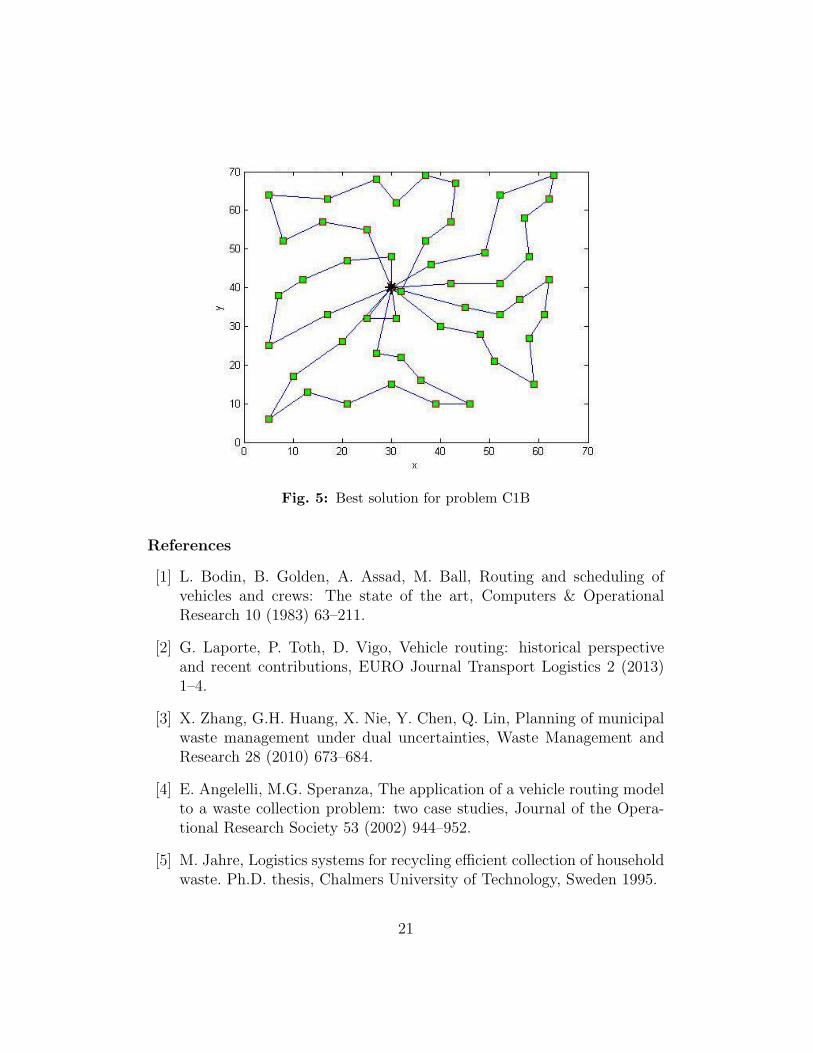
Fig. 5: Best solution for problem C1B

References

[1] L. Bodin, B. Golden, A. Assad, M. Ball, Routing and scheduling ofvehicles and crews: The state of the art, Computers & OperationalResearch 10 (1983) 63–211.

[2] G. Laporte, P. Toth, D. Vigo, Vehicle routing: historical perspectiveand recent contributions, EURO Journal Transport Logistics 2 (2013)1–4.

[3] X. Zhang, G.H. Huang, X. Nie, Y. Chen, Q. Lin, Planning of municipalwaste management under dual uncertainties, Waste Management andResearch 28 (2010) 673–684.

[4] E. Angelelli, M.G. Speranza, The application of a vehicle routing modelto a waste collection problem: two case studies, Journal of the Opera-tional Research Society 53 (2002) 944–952.

[5] M. Jahre, Logistics systems for recycling efficient collection of householdwaste. Ph.D. thesis, Chalmers University of Technology, Sweden 1995.

21

[6] S. Apotheker, Kerbside collection: Complete separation versus commin-gled collection, Resource Recycling (1990) October

[7] B. Platt, J. Zachary, Co-collection of recyclables and mixed waste: Prob-lems and opportunities, Institute for Local Self-Reliance, ILSR Washing-ton, DC, 1992.

[8] D. Pisinger, S. Ropke, A general heuristic for vehicle routing problems,Computers & Operational Research 34 (2007) 2403–2435.

[9] N. Christofides, A. Mingozzi, P. Toth, The vehicle routing problem, in:N. Christofides (Ed.), Summer School in Combinatorial Optimization,Wiley, 1979, pp. 315–338.

[10] N. Christofides, S. Eilon, An algorithm for the Vehicle-dispatching prob-lem, Journal of the Operational Research Society 20 (1969) 309–318.

[11] E. Taillard, Parallel iterative search methods for vehicle routing prob-lems, Networks 23 (1993) 661–673.

[12] M. Genreau, A. Hertz, L. Laporte, A tabu search heuristic for the vehiclerouting problem, Management Science 40 (1994) 1276–1290.

[13] I.H. Osman, Metastrategy simulated annealing and tabu search algo-rithms for the vehicle routing problem, Annals of Operational research41 (1993) 421–451.

[14] S.R. Thangiah, A hybrid genetic algorithms, simulated annealing andtabu search heuristic for vehicle routing problems with time windows,in: L. Chambers (Ed.), Practical Handbook of Genetic Algorithms, vol.III: Complex Structures, CRC Press, 1999, pp. 347–381.

[15] B.M. Baker, M.A. Ayechew, A genetic algorithm for the vehicle routingproblem, Computers & Operational Research 30 (2003) 787–800.

[16] C. Prins, A simple and effective evolutionary algorithm for the vehiclerouting problem, Computers & Operational Research 31 (2004) 1985–2002.

[17] K.C. Tan, Y.H. Chew, L.H. Lee, A Hybrid multi-objective evolution-ary algorithm for solving vehicle routing problem with time windows,Computational Optimization and Applications 34 (2005) 115–151.

22

[18] B. Ombuki, B.J. Ross, F. Hanshar, Multi-objective genetic algorithmsfor vehicle routing problem with time windows, Applied Intelligence 24(2006) 17–30.

[19] K. Ghoseiri, S.F. Ghannadpour, Multi-objective vehicle routing prob-lem with time windows using goal programming and genetic algorithm,Applied Soft Computing 10 (2010) 1096–1107.

[20] Z. Ursani, D. Essam, D. Cornforth, R. Stocker, Localised genetic al-gorithm for vehicle routing problem with time windows, Applied SoftComputing 11 (2011) 5375–5390.

[21] M.R. Khouadjia, B. Sarasola, E. Alba, L. Jourdan, E.-G. Talbi, A com-parative study between dynamic adapted PSO and VNS for the vehiclerouting problem with dynamic requests, Applied Soft Computing 12(2012) 1426–1439.

[22] M. Dorigo, T. Stutzle, Ant Colony Optimization, MIT Press, USA, 2004.

[23] S. Mazzeo, I. Loiseau, An ant colony algorithm for the capacitated vehi-cle routing problem, Electronic Notes in Discrete Mathematics 18 (2004)181–186.

[24] N.V. Karadimas, K. Papatzelou, V.G. Loumos, Optimal solid wastecollection routes identified by the ant colony system algorithm, WasteManagement and Research 25 (2007) 139–147.

[25] N.V. Karadimas, G. Kouzas, I. Anagnostopoulos, V. Loumos, Urbansolid waste collection and routing: the ant colony strategic approach,International Journal of Simulation: Systems, Science and Technology6 (2007) 45–53.

[26] J.E. Bell, P.R. McMullen, Ant colony optimization techniques for thevehicle routing problem, Advanced Engineering Informatics 18 (2004)41–48.

[27] J. Bautista, J. Pereira, Ant algorithms for urban waste collection rout-ing, Lecture Notes in Computer Science 3172 (2004) 386–403.

[28] A.E. Rizzoli, R. Montemanni, E. Lucibello, L.M. Gambardella, Antcolony optimization for real-world vehicle routing problems, Swarm In-telligence 1 (2007) 135–151.

23

[29] X. Zhang, L. Tang, A new hybrid ant colony optimization algorithmfor the vehicle routing problem, Pattern Recognition Letters 30 (2009)848–855

[30] M. Reimann, M. Stummer, K. Doerner, A savings based ant system forthe vehicle routing problem, in: Proceedings of the Genetic and Evolu-tionary Computation Conference, Morgan Kaufmann Publishers, USA,2002, pp. 1317–1326.

[31] M. Reimann, K. Doerner, R. Hartl, D-ants: savings-based ants divideand conquer the vehicle routing problem, Computers & Operations Re-search 31 (2004) 563–591.

[32] M. Reimann, S. Shtovba, E. Nepomuceno, A hybrid ant colony opti-mization and genetic algorithm approach for vehicle routing problemssolving, Student Papers of Complex Systems Summer School-2001, Bu-dapest (2001) 134–141.

[33] L. Van der Brugen, R. Gruson, M. Salomon, Reconsidering the distri-bution of gasoline products for a large oil company, European Journalof Operation Research, 81 (1995) 460–473.

[34] P. Avella, M. Boccia, A. Sforza, Solving a fuel delivery problem byheuristic and exact approaches, European Journal of Operational Re-search, 152 (2004) 170–179.

[35] E.D. Chajakis, M. Guignard, Scheduling deliveries in vehicles with mul-tiple compartments, Journal of Global Optimisation, 26 (2003) 43–78.

[36] A. El Fallahi, C. Prins, R. Wolfler Calvo, A memetic algorithm and atabu search for the multi-compartment vehicle routing problem, Com-puters & Operations Research, 35 (2008) 1725–1741.

[37] B. Bullnheimer, R.F. Hartl, C. Strauss, An improved ant system algo-rithm for the vehicle routing problem, Annals of Operations Research,89 (1999) 319–328.

[38] M. Muyldermans, G. Pang, On the benefits of co-collection: Experi-ments with a multi-compartment vehicle routing algorithm, EuropeanJournal of Operational Research 206 (2010) 93–103.

24

[39] S. Sahoo, S. Kim, B.I. Kim, B. Kraas, A. Popov Jr., Routing optimiza-tion for waste management, Interfaces 35 (2005) 24–36.

[40] R. Evering, Optimising a Waste Collection Service, MSc Project Report,Dept. of Mathematical Sciences, University of Bath, UK, 2011.

[41] A. Yiannakou, An extended model of the recycling waste collection pro-cess, MSc Project Report, Dept. of Mathematical Sciences, Universityof Bath, UK, 2012.

[42] E. Bonabeau, M. Dorigo, G. Theraulaz, Swarm intelligence: from natu-ral to artificial systems. Oxford University Press, USA 1999.

25