An Analytical Solution for Voltage Stability Studies ... · reactive power capability of wind...

J Electr Eng Technol.2015; 10(?): 30-40 http://dx.doi.org/10.5370/JEET.2015.10.2.030

30

Copyright ⓒ The Korean Institute of Electrical Engineers This is an Open-Access article distributed under the terms of the Creative Commons Attribution Non-Commercial License (http://creativecommons.org/

licenses/by-nc/3.0/)which permits unrestricted non-commercial use, distribution, and reproduction in any medium, provided the original work is properly cited.

An Analytical Solution for Voltage Stability Studies Incorporating Wind Power

Yu-Zhang Lin*, Li-Bao Shi*, Liang-Zhong Yao**, Yi-Xin Ni*, Shi-Yao Qin**, Rui-Ming Wang**, and Jin-Ping Zhang**†

Abstract – Voltage stability is one of the most critical security issues which has not yet been well resolved to date. In this paper, an analytical method called PQ plane analysis with consideration of the reactive power capability of wind turbine generator and the wake effect of wind farm is proposed for voltage stability study. Two voltage stability indices based on the proposed PQ plane analysis method incorporating the uncertainties of load-increasing direction and wind generation are designed and implemented. Cases studies are conducted to investigate the impacts of wind power incorporation with different control modes. Simulation results demonstrate that the constant voltage control based on reactive power capability significantly enhances voltage stability in comparison of the conventional constant power factor control. Some meaningful conclusions are obtained.

Keywords: Voltage stability, PQ plane, Wind power, Reactive power capability

1. Introduction In the recent decades, a few serious power system

contingencies occurring around the world pertinent to voltage collapse have drawn wide attentions for electrical engineers [1-2]. Over the years, a variety of analyzing methods have been proposed to give insight into the mechanism and assessment of voltage stability. However, due to the complexity of this issue, it is difficult for these attempts to provide the comprehensive and time-saving solutions.

The existing analyzing methods can be classified into two categories: static and dynamic. So far, the static methods, which can give instructive information for power system planning, operation and control with ignorance of transient behavior, are widely applied in utilities. Especially, the conventional PV and QV curves based analysis methods [3-6], which are applied to investigate the relationships between voltage and active or reactive power in a specific load increasing direction, are very useful in determining voltage stability margin and developing remedial action strategies. However, such methods are only applicable for certain increasing modes and cannot provide a full view of voltage stability. On the other hand, the utilized continuation power flow technique is rather time-consuming. Furthermore, with the integration of large-scale renewable energy sources, especially for wind power, the

new challenges and issues to the voltage stability will appear in the smart grid environment. Three factors, the variability and intermittency of wind energy, the wind turbine generator (WTG) models, and the pattern of grid-connection, should be taken into account for voltage stability studies incorporating wind power [7-9]. In a nutshell, how to effectively conduct the voltage stability analysis incorporating intermittent wind power and develop more powerful analysis tool become very imperative and necessary.

In this paper, an analytical method called as PQ Plane analysis, is proposed for voltage stability studies incur-porating wind power. Two factors, the reactive power capability of WTG and the wake effect of wind farm, are paid special attention to during the modelling of wind farms of doubly-fed induction generator (DFIG) type. The stability boundary and voltage distribution are derived and shown on the PQ plane. Furthermore, a set of indices are defined to indicate the voltage security situation of a load bus. The proposed method is derived in a single-load-infinite-bus system, and can be easily expanded to complex power systems by applying Thevenin Equivalent Circuits [10] or the newly proposed Coupled Single-Port Circuits [11]. Some preliminary and meaningful conclusions are drawn.

The rest of the paper is organized as follows: In Section 2, the static modelling of wind farm involving the reactive power capability of DFIG and the wake effect is discussed. The PQ plane analysis method incorporating wind generation is proposed and detailed in Section 3. The case studies with different simulation scenarios are carried out in Section 4. The conclusions and research prospects can be found in Section 5.

† Corresponding Author: National Key Laboratory of Power System in Shenzhen, Graduate School at Shenzhen, Tsinghua University, Shenzhen 518055, China. ([email protected])

* National Key Laboratory of Power System in Shenzhen, Graduate School at Shenzhen, Tsinghua University, Shenzhen 518055, China. ([email protected])

** China Electric Power Research Institute, Qinghe, Beijing 100192, China. ([email protected])

Received: March 13, 2014; Accepted: January 14, 2014

ISSN(Print) 1975-0102ISSN(Online) 2093-7423

Yu-Zhang Lin, Li-Bao Shi, Liang-Zhong Yao, Yi-Xin Ni, Shi-Yao Qin, Rui-Ming Wang and Jin-Ping Zhang

http://www.jeet.or.kr │ 31

2. Modelling of Wind Farms for Voltage Stability Studies

In this section, a static model of wind farm of DFIG type

is proposed with consideration of reactive power capability and wake effect.

2.1 Active power output of wind farms with consid-

eration of wake effect The active power output of a DFIG Pwt with respect to

the wind speed v can be expressed as [12]

3 3

3 3

0 ( or )

( )

( )

ci co

ciwt wtr ci r

r ci

wtr r

v v v v

v vP P v v v

v v

P v v

< ≥

−= ≤ ≤

−

≥

⎧⎪⎪⎨⎪⎪⎩

(1)

where vci, vco, vr and Pwtr are cut-in speed, cut-out speed, rated speed and rated active power, respectively.

In conventional model of wind farm, the wind speed each wind turbine captures is assumed to be the same. Actually, in practical wind farms, the wind turbines located downwind gain a lower wind speed than those located upwind, in that the kinetic energy of wind is partly consumed by the latter ones. Such aforementioned situation is called as wake effect. A lot of wake effect models have been developed to date with specific applicability. In this paper, the Jensen Model [13], as illustrated in Fig. 1 is applied to describe the wake effect in a wind farm located on flat terrain. In accordance with the Jensen model, the wind speed behind a wind turbine vwake with respect to the distance from the wind turbine plane x can be presented as

2

1( ) 1 (1 1 ) wtwake T

wt x

Rv x v

R xξ

ξ= − − −

+

⎡ ⎤⎛ ⎞⎢ ⎥⎜ ⎟

⎝ ⎠⎢ ⎥⎣ ⎦ (2)

where v1 is the original wind speed; Rwt is the wind turbine

radius; ξx is the damping coefficient; and ξT is the thrust coefficient of the wind turbine. ξx can be obtained by 0tan ( ) / ( )x wake wake wakek v xξ α σ σ= = + (3)

where kw is the turbulence intensity, which can be estimated empirically; σwake and σ0 are mean-square deviation of natural turbulence and turbulence caused by WTGs, respectively.

For a wind farm with nrow rows and ncol columns in a chessboard-pattern layout, the distance between two adjacent rows of WTGs is drow, the wind speed in the ith row can be calculated by

( 1)

1 ( 1 )i

i d rowv v i nξ −= = L (4)

where v1 is the wind speed in the first row (the original wind speed), and ξd is the damping coefficient between two adjacent rows of WTGs, which is given by

( )2

1 1 1 Td T

T x row

R

R dξ ξ

ξ= − − −

+

⎛ ⎞⎜ ⎟⎝ ⎠

(5)

Then the active power output of a single DFIG in the ith

row Pwt,i can be calculated based on Eq. (1). Ignoring the losses in the collection systems, the total output of a wind farm equipped with DFIG is

,1

rown

wf col wt ii

P n P=

= ∑ (6)

Fig. 2 illustrates the active power output of a wind farm

with and without considering the wake effect.

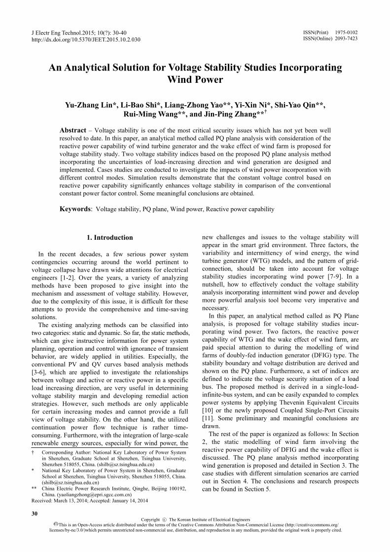
2.2 Reactive power capability curve of DFIG The equivalent circuit of a DFIG is given in Fig. 3, in

Fig. 1. The wake effect of wind turbines

0 2 4 6 8 10 12 14 16 18 20

0

0.2

0.4

0.6

0.8

1

Fig. 2. Active power output of wind farms with respect to

wind speed


32 │ J Electr Eng Technol.2015;10(1): 30-40

which the stator voltage sV& , stator current sI& , rotor voltage rV& and rotor current rI& are restricted by

( ) ( )s s r m s r sR jX I jX I I V+ + + =& & & & (7)

( )r rr r m s r

R VjX I jX I I

s s+ + + =⎛ ⎞

⎜ ⎟⎝ ⎠

&& & & (8)

where s is the slip ratio.

From (7) and (8), we have

s

s

rr

VI

Y VI

s

= ⋅⎡ ⎤⎡ ⎤ ⎢ ⎥⎢ ⎥ ⎢ ⎥⎣ ⎦ ⎣ ⎦

&&

&&

(9)

s

s

rr

IV

GVI

s

= ⋅⎡ ⎤ ⎡ ⎤⎢ ⎥ ⎢ ⎥⎢ ⎥ ⎣ ⎦⎣ ⎦

&&

&&

(10)

r

s

sr

VV

BsI

I= ⋅

−

⎡ ⎤ ⎡ ⎤⎢ ⎥ ⎢ ⎥⎢ ⎥ ⎣ ⎦⎣ ⎦

&&

&&

(11)

where matrix Y, G and B can be derived from the parameters of the equivalent circuit.

The complex power outputs of the stator and rotor are expressed as

s s sS V I= −& & (12)

r r rS V I= −& & (13) If the losses in the boosting transformer are negligible,

the total power output can be given by

( )tot s s r gcS P jQ P jQ= + + +& (14)

where Ps is the stator active power; Qs is the stator reactive power; Pr is the rotor active power; Qgc is the grid-side convertor reactive power.

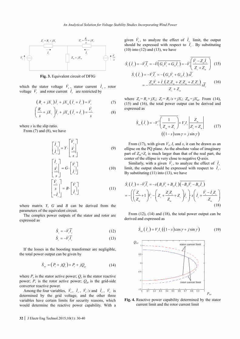
Among the four variables, sV& , sI& , rV& /s and rI& , sV& is determined by the grid voltage, and the other three variables have certain limits for security reasons, which would determine the reactive power capability. With a

given sV& , to analyze the effect of rI& limit, the output should be expressed with respect to rI& . By substituting (10) into (12) and (13), we have

( ) ( )11 12s m r

s r s s s r s

s m

V Z IS I V I V G V G I V

Z Z

−= − = − + = −

+

⎛ ⎞⎜ ⎟⎝ ⎠

& && & & & & & & (15)

( ) ( )( )

21 22r r r r s r r

m s r r m s m s rr

s m

S I V I G V G I sI

Z V I Z Z Z Z Z ZsI

Z Z

= − = − +

+ + += −

+

& & & & &

& & (16)

where Zs = Rs + jXs; Zr = Rr /s + jXr; Zm = jXm. From (14), (15) and (16), the total power output can be derived and expressed as

( )

( )( )

2 1

1 cos sin

mtot r s s r

m s s m

ZS I V V I

Z Z Z Z

s jγ γ

= − ++ +

− +

⎛ ⎞⎜ ⎟⎝ ⎠

& & (17)

From (17), with given Vs, Ir and s, it can be drawn as an

ellipse on the PQ plane. As the absolute value of imaginary part of Zm+Zs is much larger than that of the real part, the center of the ellipse is very close to negative Q-axis.

Similarly, with a given sV& , to analyze the effect of sI& limit, the output should be expressed with respect to sI& . By substituting (11) into (13), we have

( ) ( )( )11 12 21 22

1

r s r r s s s s

s r s s srs r s s s

m m m

S I V I s B V B I B V B I

Z Z V I ZZV Z Z I s I

Z Z Z

= − = − + − −

−= − + − + + +

⎛⎛ ⎞ ⎛ ⎞ ⎞ ⎛ ⎞⎜⎜ ⎟ ⎜ ⎟ ⎟ ⎜ ⎟⎝⎝ ⎠ ⎝ ⎠ ⎠ ⎝ ⎠

⋅

& & & & & & &

& && & &

(18) From (12), (14) and (18), the total power output can be

derived and expressed as

( ) ( )( )1 cos sintot s s sS I V I s jγ γ= − +& & (19)

Qwt

Pwt

stator current limit

rotor current limit

Fig. 4. Reactive power capability determined by the stator

current limit and the rotor current limit

rVs

&sV&

sI& rI&

s s sZ R jX= + rr r

RZ jXs

= +

m mZ jX=

Fig. 3. Equivalent circuit of DFIG



Fig. 4 shows the reactive power capability determined by limits of the stator current and rotor current. The solid line given in Fig. 4 denotes the reactive power capability with respect to the active power output.

As mentioned above, the slip ratio s is assumed to be constant. In actual operation of DFIGs, however, the rotational speed of the wind turbine changes with the wind speed to capture the maximum power. A commonly-applied speed control law is given as follows [15]:

min 1

3 1 2

1 2 3

max 11 3 3

max 3

0

( )

( )

wt

wtwt

opt

wt

wt

wt wt r

n P P

PP P P

kn f P

n P P P

n nn P P P P P

P P

< ≤

< ≤

= =< ≤

−+ − < ≤

−

⎧⎪⎪⎪⎪⎨⎪⎪⎪⎪⎩

(20)

where nmin is the minimum speed; n1 is the synchronous speed; nmax is the maximum speed; kopt is the power adjustment coefficient; P1, P2 and P3 are three demarcation points, respectively.

As the slip ratio changes, the shape of the reactive power capability curve will change. The corresponding solution procedures are given as follows: 1) Assign the initial active power P0=0 and the increment

ΔP; Let i=1; 2) Pi=P0+iΔP; 3) Calculate rotational speed ni according to Eq. (20); 4) Calculate slip ratio si; 5) Calculate the reactive power upper limit Qmax,i and

lower limit Qmin,i according to Eq. (17) and (19) respectively;

6) If Qmax,i≤Qmin,i or Pi≥1, go to Step 7; else, i=i+1, go to Step 2;

7) Plot the reactive power capability curve. The reactive power capability curves with different s are

given in Fig. 5. It can be seen that as the slip ratio decreases or the rotational speed increases, the operation region expands and the reactive power capability increases. The actual reactive power capability curve is made up of points in different curves. When P < P1 and P2 ≤ P < P3, the actual reactive power capability curve will overlap curves with s=0.3 and s=0 respectively. In other areas, it crosses a set of curves with constant s as the slip ratio keeps changing.

2.3 Reactive power capability curve of wind farm

and voltage control strategies With the consideration of the wake effect, the total

power output of wind farm of DFIG-type can be calculated according to the following procedures:

1) Assign the initial wind speed v0=0 and the increment Δv; Let k=1;

2) vk=v0+kΔv; 3) Calculate the wind speeds vki according to Eqs. (4) and

(5); 4) Calculate the active output of DFIGs in each row

Pwt,ki according to Eq. (1); 5) Calculate the active output of the whole wind farm

Pwf,k according to Eq. (6); 6) Calculate the rotational speeds of DFIGs in each row

nki according to Eq. (20); 7) Calculate the slip ratios of DFIGs in each row ski; 8) Calculate the reactive power upper limit Qwtmax,ki

and lower limit Qwtmin,ki of DFIGs in each row according to Eqs. (17) and (19), respectively;

9) Calculate the reactive power upper limit Qwfmax,ki and lower limit Qwfmin,ki of the whole wind farm according to the following Equations

max max,1

rown

wf col wt ii

Q Qn=

= ∑ (21)

min min,1

rown

wf col wt ii

Q Qn=

= ∑ (22)

10) If vi≥vco, go to Step 11; else, i=i+1, go to Step 2; 11) Plot the reactive power capability curve.

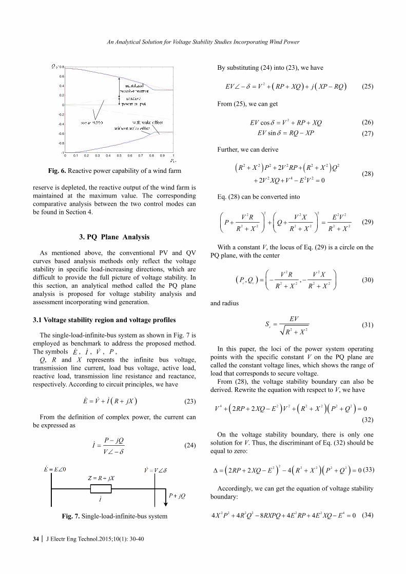
Fig. 6 shows the reactive power capability of a wind

farm with/without consideration of the wake effect as well as the conventional constant power factor control strategy.

From Fig. 6, with conventional control strategy, there is a large amount of reactive reserve unutilized, especially when the active power output is relatively low. To make full use of the reactive reserve for the sake of voltage security enhancement, the constant voltage control mode is applied in this paper. When there is an amount of reactive reserve, the voltage at the point of common coupling (PCC) is maintained at 1 p.u.; when the reactive

0 0.1 0.2 0.3 0.4 0.5 0.6 0.7 0.8 0.9 1-1

-0.5

0

0.5

0 0.1 0.2 0.3 0.4 0.5 0.6 0.7 0.8 0.9 1

-0.4

-0.2

0

0.2

0.4

0 0.1 0.2 0.3 0.4 0.5 0.6 0.7 0.8 0.9 1

-0.4

-0.2

0

0.2

0.4

Fig. 5. Capability curves with different constant s and with

the speed control law



reserve is depleted, the reactive output of the wind farm is maintained at the maximum value. The corresponding comparative analysis between the two control modes can be found in Section 4.

3. PQ Plane Analysis As mentioned above, the conventional PV and QV

curves based analysis methods only reflect the voltage stability in specific load-increasing directions, which are difficult to provide the full picture of voltage stability. In this section, an analytical method called the PQ plane analysis is proposed for voltage stability analysis and assessment incorporating wind generation.

3.1 Voltage stability region and voltage profiles

The single-load-infinite-bus system as shown in Fig. 7 is

employed as benchmark to address the proposed method. The symbols E& , I& , V& , P ,

Q, R and X represents the infinite bus voltage, transmission line current, load bus voltage, active load, reactive load, transmission line resistance and reactance, respectively. According to circuit principles, we have

( )E V I R jX= + +& & & (23)

From the definition of complex power, the current can

be expressed as

P jQ

IV δ

−=

∠ −& (24)

By substituting (24) into (23), we have

( ) ( )2EV V RP XQ j XP RQδ∠ − = + + + − (25) From (25), we can get

2cosEV V RP XQδ = + + (26)

sinEV RQ XPδ = − (27) Further, we can derive

( ) ( )2 2 2 2 2 2 2

2 4 2 2

2

2 0

R X P V RP R X Q

V XQ V E V

+ + + +

+ + − = (28)

Eq. (28) can be converted into

2 22 2 2 2

2 2 2 2 2 2

V R V X E VP Q

R X R X R X+ + + =

+ + +

⎛ ⎞ ⎛ ⎞⎜ ⎟ ⎜ ⎟⎝ ⎠ ⎝ ⎠

(29)

With a constant V, the locus of Eq. (29) is a circle on the

PQ plane, with the center

( )2 2

2 2 2 2, ,c c

V R V XP Q

R X R X= − −

+ +

⎛ ⎞⎜ ⎟⎝ ⎠

(30)

and radius

2 2

r

EVS

R X=

+ (31)

In this paper, the loci of the power system operating

points with the specific constant V on the PQ plane are called the constant voltage lines, which shows the range of load that corresponds to secure voltage.

From (28), the voltage stability boundary can also be derived. Rewrite the equation with respect to V, we have

( ) ( )( )4 2 2 2 2 2 22 2 0V RP XQ E V R X P Q+ + − + + + = (32)

On the voltage stability boundary, there is only one

solution for V. Thus, the discriminant of Eq. (32) should be equal to zero:

( ) ( )( )22 2 2 2 22 2 4 0RP XQ E R X P QΔ = + − − + + = (33)

Accordingly, we can get the equation of voltage stability

boundary:

2 2 2 2 2 2 44 4 8 4 4 0X P R Q RXPQ E RP E XQ E+ − + + − = (34)

0 0.1 0.2 0.3 0.4 0.5 0.6 0.7 0.8 0.9 1-1

-0.8

-0.6

-0.4

-0.2

0

0.2

0.4

0.6

0.8

Fig. 6. Reactive power capability of a wind farm

Fig. 7. Single-load-infinite-bus system



The discriminant of Eq. (34) equals to zero, indicating that the voltage stability boundary is a parabola on the PQ plane.

Fig. 8 displays the voltage stability boundary and a set of constant voltage lines pertinent to the single-load-infinite-bus system in which X is much larger than R. It can be seen that the stability boundary is a parabola. The parts inside the parabola are the stability region. The constant voltage lines are circles tangent to the stability boundary, i.e. the stability boundary is the envelope of all constant voltage lines.

For a load bus, only the first quadrant of PQ plane as shown in Fig. 9 needs to be elaborately studied. It can be seen from Fig. 9 that the voltage constant lines do not intersect in the first quadrant. As the load increases, the operating point moves closer to the stability boundary and the bus experiences a voltage dip. Furthermore, it can also be found that the information provided by PV and QV curves based analysis methods is easily included in PQ plane. For instance, the PV curve based analysis method assumes that the load increases with a given power factor cosφ, and calculates the active power margin to the stability boundary ΔPL. On the PQ plane, the load increasing direction is represented as the direction of AB

uuur,

and ΔPL is the length of AC. The QV curve based analysis methods assumes that there is a synchronous condenser

installed at the load bus and investigates the relationship between V and Q while maintaining P constant. On the PQ plane, the increasing direction is represented as the direction of AD

uuur, and the reactive power margin ΔQc is the

length of AD.

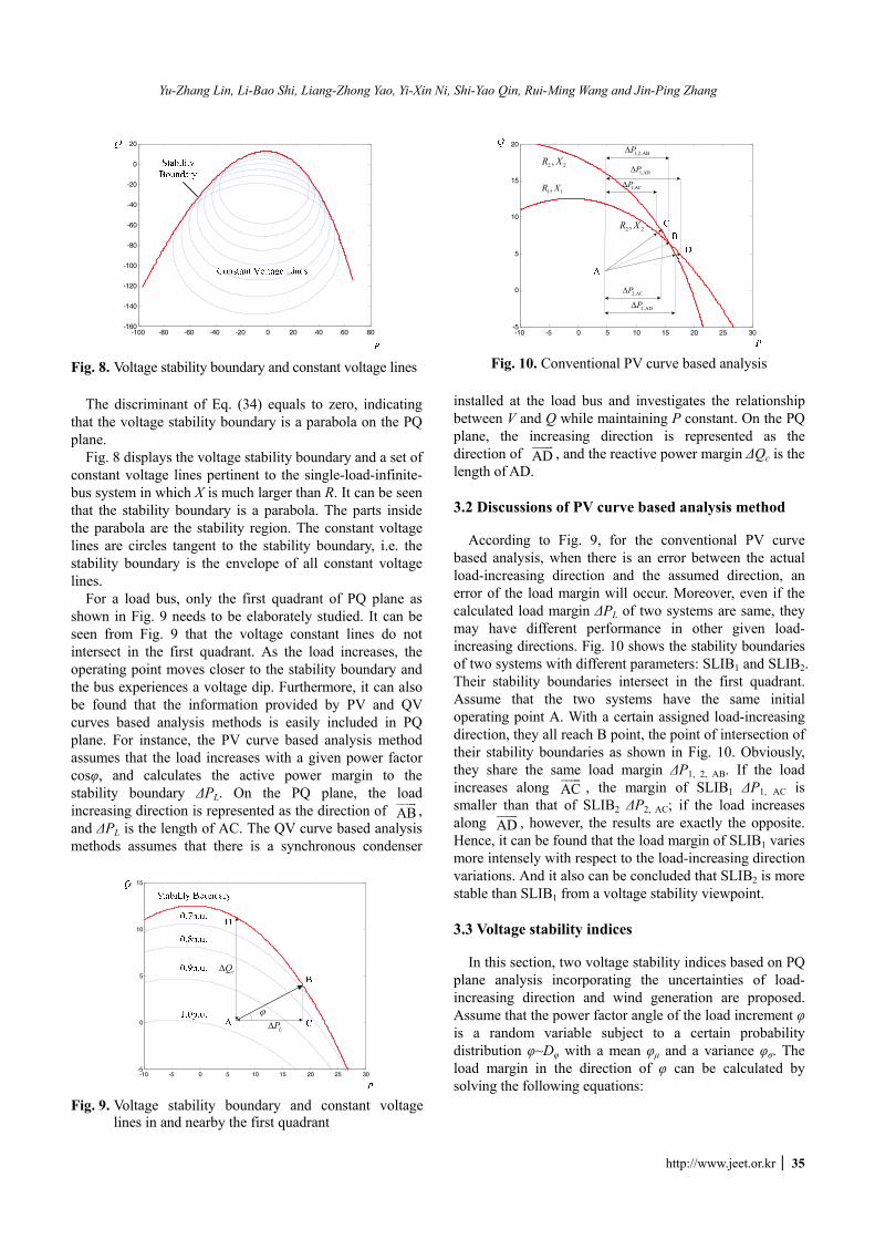
3.2 Discussions of PV curve based analysis method According to Fig. 9, for the conventional PV curve

based analysis, when there is an error between the actual load-increasing direction and the assumed direction, an error of the load margin will occur. Moreover, even if the calculated load margin ΔPL of two systems are same, they may have different performance in other given load-increasing directions. Fig. 10 shows the stability boundaries of two systems with different parameters: SLIB1 and SLIB2. Their stability boundaries intersect in the first quadrant. Assume that the two systems have the same initial operating point A. With a certain assigned load-increasing direction, they all reach B point, the point of intersection of their stability boundaries as shown in Fig. 10. Obviously, they share the same load margin ΔP1, 2, AB. If the load increases along AC

uuur, the margin of SLIB1 ΔP1, AC is

smaller than that of SLIB2 ΔP2, AC; if the load increases along AD

uuur, however, the results are exactly the opposite.

Hence, it can be found that the load margin of SLIB1 varies more intensely with respect to the load-increasing direction variations. And it also can be concluded that SLIB2 is more stable than SLIB1 from a voltage stability viewpoint.

3.3 Voltage stability indices

In this section, two voltage stability indices based on PQ

plane analysis incorporating the uncertainties of load-increasing direction and wind generation are proposed. Assume that the power factor angle of the load increment φ is a random variable subject to a certain probability distribution φ~Dφ with a mean φμ and a variance φσ. The load margin in the direction of φ can be calculated by solving the following equations:

-100 -80 -60 -40 -20 0 20 40 60 80-160

-140

-120

-100

-80

-60

-40

-20

0

20

Fig. 8. Voltage stability boundary and constant voltage lines

-10 -5 0 5 10 15 20 25 30-5

0

5

10

15

20

1,ADPΔ

1,ACPΔ

2,ACPΔ

2,ADPΔ

1,2,ABPΔ2 2,R X

2 2,R X

1 1,R X

Fig. 10. Conventional PV curve based analysis

-10 -5 0 5 10 15 20 25 30-5

0

5

10

15

LPΔ

cQΔ

ϕ

Fig. 9. Voltage stability boundary and constant voltage

lines in and nearby the first quadrant



( )

2 2 2 2 2 2 4

0 0

4 4 8 4 4 0

tan

X P R Q RXPQ E RP E XQ E

P P Q Qϕ

+ − + + − =

− = −

⎧⎨⎩

(35) Two solutions can be obtained from (35), and only the

solution named Pmargin in the first quadrant is retained. As Pmargin is a function of φ:

( )marginP f ϕ= (36)

It must subject to a certain probability distribution

Pmargin~ DPmargin. In our work, the mean and variance of Pmargin are calculated approximately to avoid the heavy computational burden. According to probability theories, with given φμ and φσ, Pmargin μ and Pmargin, σ can be estimated respectively by

( ) ( ) 2

,

1

2marginP f f''μ μ μ σϕ ϕ ϕ≈ + (37)

( ),marginP f'σ μ σϕ ϕ≈ (38)

where f’(φμ) and f’’(φμ) can be estimated by difference quotients. Assign a small increment, and substitute φ=φμ-Δφ and φ=φμ+Δφ into Eq. (36) to get f(φμ-Δφ) and f(φμ+Δφ). Then f’(φμ) and f’’(φμ) can be calculated by

( ) ( ) ( )2

f ff' μ μ

μ

ϕ ϕ ϕ ϕϕ

ϕ

+ Δ − − Δ≈

Δ (39)

( ) ( ) ( ) ( )2

2f f ff'' μ μ μ

μ

ϕ ϕ ϕ ϕ ϕϕ

ϕ

+ Δ − + − Δ≈

Δ (40)

The coefficient of variation of Pmargin can be calculated

by

,,

,

100%marginmargin CV

margin

PP

Pσ

μ

= × (41)

We define Pmargin,μ and Pmargin,CV as voltage stability

indices, called the Mean Margin to Voltage Instability (MMVI) and the Variation Margin to Voltage Instability (VMVI) respectively. MMVI represents the expectation of the load margin. The larger the index, the more secure the system. VMVI represents the variance of the load margin. The larger the index, the less robust the system is to the randomness of the load.

Conventionally, the solutions of voltage stability analysis mainly focus on how the current state is to the stability boundary. In fact, voltage violation is also an important issue that needs to be considered in practical operation. As the initial operating point and the load-increasing direction vary, there does not exist a fixed relationship between the distance to voltage instability and the distance to voltage

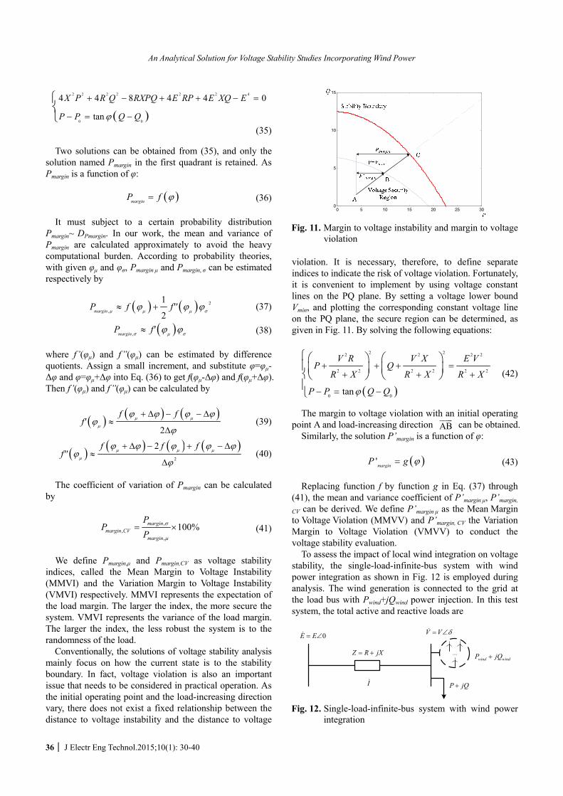
violation. It is necessary, therefore, to define separate indices to indicate the risk of voltage violation. Fortunately, it is convenient to implement by using voltage constant lines on the PQ plane. By setting a voltage lower bound Vmin, and plotting the corresponding constant voltage line on the PQ plane, the secure region can be determined, as given in Fig. 11. By solving the following equations:

( )

2 22 2 2 2

2 2 2 2 2 2

0 0tan

V R V X E VP Q

R X R X R X

P P Q Qϕ

+ + + =+ + +

− = −

⎧⎛ ⎞ ⎛ ⎞⎪⎜ ⎟ ⎜ ⎟⎨⎝ ⎠ ⎝ ⎠⎪⎩

(42)

The margin to voltage violation with an initial operating

point A and load-increasing direction ABuuur

can be obtained. Similarly, the solution P’margin is a function of φ:

( )'marginP g ϕ= (43) Replacing function f by function g in Eq. (37) through

(41), the mean and variance coefficient of P’margin μ, P’margin,

CV can be derived. We define P’margin μ as the Mean Margin to Voltage Violation (MMVV) and P’margin, CV the Variation Margin to Voltage Violation (VMVV) to conduct the voltage stability evaluation.

To assess the impact of local wind integration on voltage stability, the single-load-infinite-bus system with wind power integration as shown in Fig. 12 is employed during analysis. The wind generation is connected to the grid at the load bus with Pwind+jQwind power injection. In this test system, the total active and reactive loads are

0 5 10 15 20 25 300

5

10

15

Fig. 11. Margin to voltage instability and margin to voltage

violation

0E E= ∠& V V δ= ∠&

I&

Z R jX= +

P jQ+

wind windP jQ+...

Fig. 12. Single-load-infinite-bus system with wind power integration



windP' P P= − (44)

windQ' Q Q= − (45) To plot voltage stability boundary and constant voltage

lines on the PQ plane based on the net load P and Q, a shift with value of (Pwind, Qwind) is added to implement the required solutions.

4. Case Studies Based on the aforementioned single-load-infinite-bus

test system shown in Fig. 7, two simulation scenarios involving the studies on the relationship between power system parameters and voltage stability and the impacts of wind farm of DFIG type on voltage stability are designed for case studies. Some meaningful conclusions are drawn based on the studies.

4.1 Impacts of key parameters of power system on

voltage stability Impacts of transmission line ratio of reactance X and

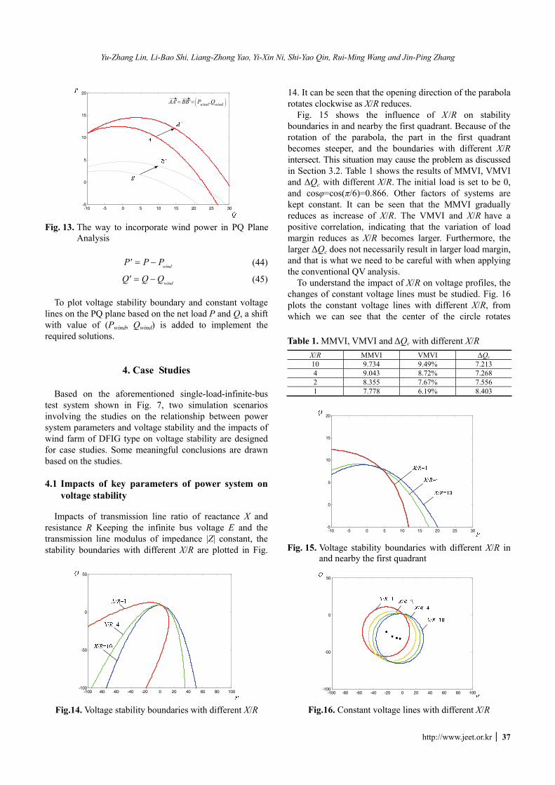
resistance R Keeping the infinite bus voltage E and the transmission line modulus of impedance |Z| constant, the stability boundaries with different X/R are plotted in Fig.

14. It can be seen that the opening direction of the parabola rotates clockwise as X/R reduces.

Fig. 15 shows the influence of X /R on stability boundaries in and nearby the first quadrant. Because of the rotation of the parabola, the part in the first quadrant becomes steeper, and the boundaries with different X/R intersect. This situation may cause the problem as discussed in Section 3.2. Table 1 shows the results of MMVI, VMVI and ΔQc with different X/R. The initial load is set to be 0, and cosφ=cos(π/6)=0.866. Other factors of systems are kept constant. It can be seen that the MMVI gradually reduces as increase of X/R. The VMVI and X/R have a positive correlation, indicating that the variation of load margin reduces as X/R becomes larger. Furthermore, the larger ΔQc does not necessarily result in larger load margin, and that is what we need to be careful with when applying the conventional QV analysis.

To understand the impact of X/R on voltage profiles, the changes of constant voltage lines must be studied. Fig. 16 plots the constant voltage lines with different X/R, from which we can see that the center of the circle rotates

Table 1. MMVI, VMVI and ΔQc with different X/R X/R MMVI VMVI ΔQc 10 9.734 9.49% 7.213 4 9.043 8.72% 7.268 2 8.355 7.67% 7.556 1 7.778 6.19% 8.403

-10 -5 0 5 10 15 20 25 30-5

0

5

10

15

20

Fig. 15. Voltage stability boundaries with different X/R in

and nearby the first quadrant

-100 -80 -60 -40 -20 0 20 40 60 80 100-100

-50

0

50

Fig.16. Constant voltage lines with different X/R

-10 -5 0 5 10 15 20 25 30-5

0

5

10

15

20

' ' ,wind windAA BB P Q⎛ ⎞⎜ ⎟⎝ ⎠

= =

Fig. 13. The way to incorporate wind power in PQ Plane

Analysis

-100 -80 -60 -40 -20 0 20 40 60 80 100-100

-50

0

50

Fig.14. Voltage stability boundaries with different X/R



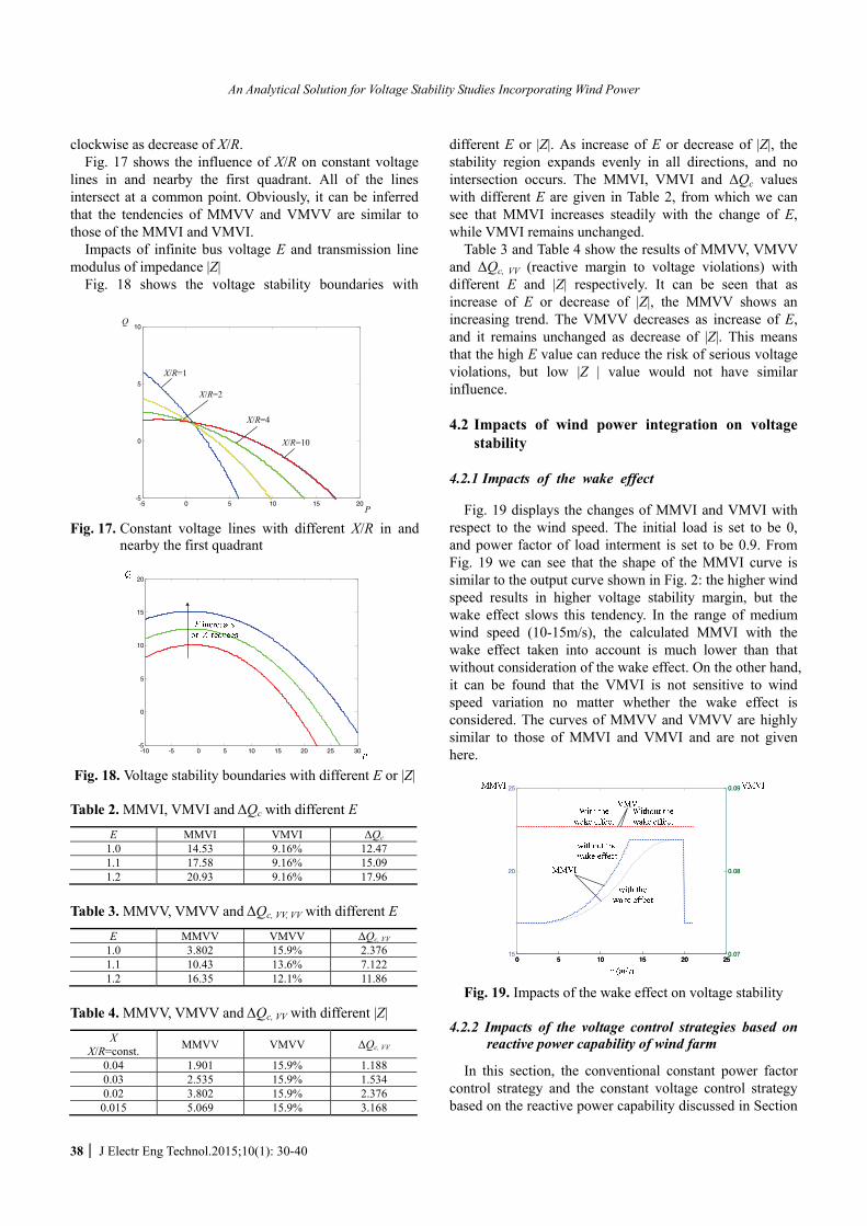
clockwise as decrease of X/R. Fig. 17 shows the influence of X/R on constant voltage

lines in and nearby the first quadrant. All of the lines intersect at a common point. Obviously, it can be inferred that the tendencies of MMVV and VMVV are similar to those of the MMVI and VMVI.

Impacts of infinite bus voltage E and transmission line modulus of impedance |Z|

Fig. 18 shows the voltage stability boundaries with

different E or |Z|. As increase of E or decrease of |Z|, the stability region expands evenly in all directions, and no intersection occurs. The MMVI, VMVI and ΔQc values with different E are given in Table 2, from which we can see that MMVI increases steadily with the change of E, while VMVI remains unchanged.

Table 3 and Table 4 show the results of MMVV, VMVV and ΔQc, VV (reactive margin to voltage violations) with different E and |Z| respectively. It can be seen that as increase of E or decrease of |Z|, the MMVV shows an increasing trend. The VMVV decreases as increase of E, and it remains unchanged as decrease of |Z|. This means that the high E value can reduce the risk of serious voltage violations, but low |Z | value would not have similar influence.

4.2 Impacts of wind power integration on voltage

stability

4.2.1 Impacts of the wake effect Fig. 19 displays the changes of MMVI and VMVI with

respect to the wind speed. The initial load is set to be 0, and power factor of load interment is set to be 0.9. From Fig. 19 we can see that the shape of the MMVI curve is similar to the output curve shown in Fig. 2: the higher wind speed results in higher voltage stability margin, but the wake effect slows this tendency. In the range of medium wind speed (10-15m/s), the calculated MMVI with the wake effect taken into account is much lower than that without consideration of the wake effect. On the other hand, it can be found that the VMVI is not sensitive to wind speed variation no matter whether the wake effect is considered. The curves of MMVV and VMVV are highly similar to those of MMVI and VMVI and are not given here.

0 5 10 15 20 2515

20

25

0 5 10 15 20 250.07

0.08

0.09

0 5 10 15 20 250.07

0.08

0.09

Fig. 19. Impacts of the wake effect on voltage stability

4.2.2 Impacts of the voltage control strategies based on reactive power capability of wind farm

In this section, the conventional constant power factor

control strategy and the constant voltage control strategy based on the reactive power capability discussed in Section

-5 0 5 10 15 20-5

0

5

10Q

P

X/R=1

X/R=10

X/R=4

X/R=2

Fig. 17. Constant voltage lines with different X/R in and

nearby the first quadrant

-10 -5 0 5 10 15 20 25 30-5

0

5

10

15

20

Fig. 18. Voltage stability boundaries with different E or |Z|

Table 2. MMVI, VMVI and ΔQc with different E

E MMVI VMVI ΔQc 1.0 14.53 9.16% 12.47 1.1 17.58 9.16% 15.09 1.2 20.93 9.16% 17.96

Table 3. MMVV, VMVV and ΔQc, VV, VV with different E

E MMVV VMVV ΔQc, VV 1.0 3.802 15.9% 2.376 1.1 10.43 13.6% 7.122 1.2 16.35 12.1% 11.86

Table 4. MMVV, VMVV and ΔQc, VV with different |Z|

X X/R=const. MMVV VMVV ΔQc, VV

0.04 1.901 15.9% 1.188 0.03 2.535 15.9% 1.534 0.02 3.802 15.9% 2.376 0.015 5.069 15.9% 3.168



2 are applied for comparisons. In the constant-voltage control mode, the power factor cosφwind=0.955.

Fig. 20 shows the voltage stability boundaries in different control modes and different wind speeds. When v=19m/s, the stability boundaries of the two control modes overlap each other, because the active power output reaches the maximum and there is no reactive power reserve left. As a result, the reactive output stays at the maximum no matter which control strategy is implemented. However, in a relatively low wind speed, the studies pertinent to different control strategies are significant. When v=8m/s, the stability boundary corresponding to constant voltage control is shifted towards the positive Q-axis direction compared with the one corresponding to constant power factor control. In the first quadrant, the shift considerably expands the stability region, and increases the stability margin. In fact, in the region nearby the load-increasing direction, the stability margin is close to that with the wind speed of 19m/s, i.e. the stability margin variation resulting from the wind speed variation is largely mitigated. The load margin gap between the high and low wind speeds situations is greatly narrowed by implementing constant voltage control strategy, so that the MMVI can maintain a relatively high value in a wide wind speed range. Fig. 22 demonstrates another advantage of applying the constant voltage control strategy: the VMVI drops greatly in the range of low wind speed, indicating

that the risk of serious voltage instability problem is reduced in a large extent.

The voltage violation issue can be studied in a similar way. The constant voltage lines in different control modes and different wind speeds are shown in Fig. 23. The impact of constant voltage control strategy on constant voltage lines is even greater: the security region with constant voltage mode and a wind speed of 8m/s entirely covers the security region with constant power factor mode the speed of 19m/s.

This phenomenon is shown more clearly in Fig. 24. With the constant voltage control, the value of MMVV in the

0 5 10 15 20 25 300

2

4

6

8

10

12

14

16

18

20

Fig. 20. Voltage stability boundaries in different control

modes and different wind speeds

0 5 10 15 20 2515

16

17

18

19

20

21

22

23

Fig. 21. MMVI with respect to wind speed in different

control modes

0 5 10 15 20 250.07

0.072

0.074

0.076

0.078

0.08

0.082

0.084

0.086

0.088

Fig. 22. VMVI with respect to wind speed in different

control modes

0 5 10 15 20 25 300

5

10

15

Fig. 23. Constant voltage lines in different control modes

and different wind speeds

0 5 10 15 20 255

6

7

8

9

10

11

12

Fig. 24. MMVV with respect to wind speed in different

control modes



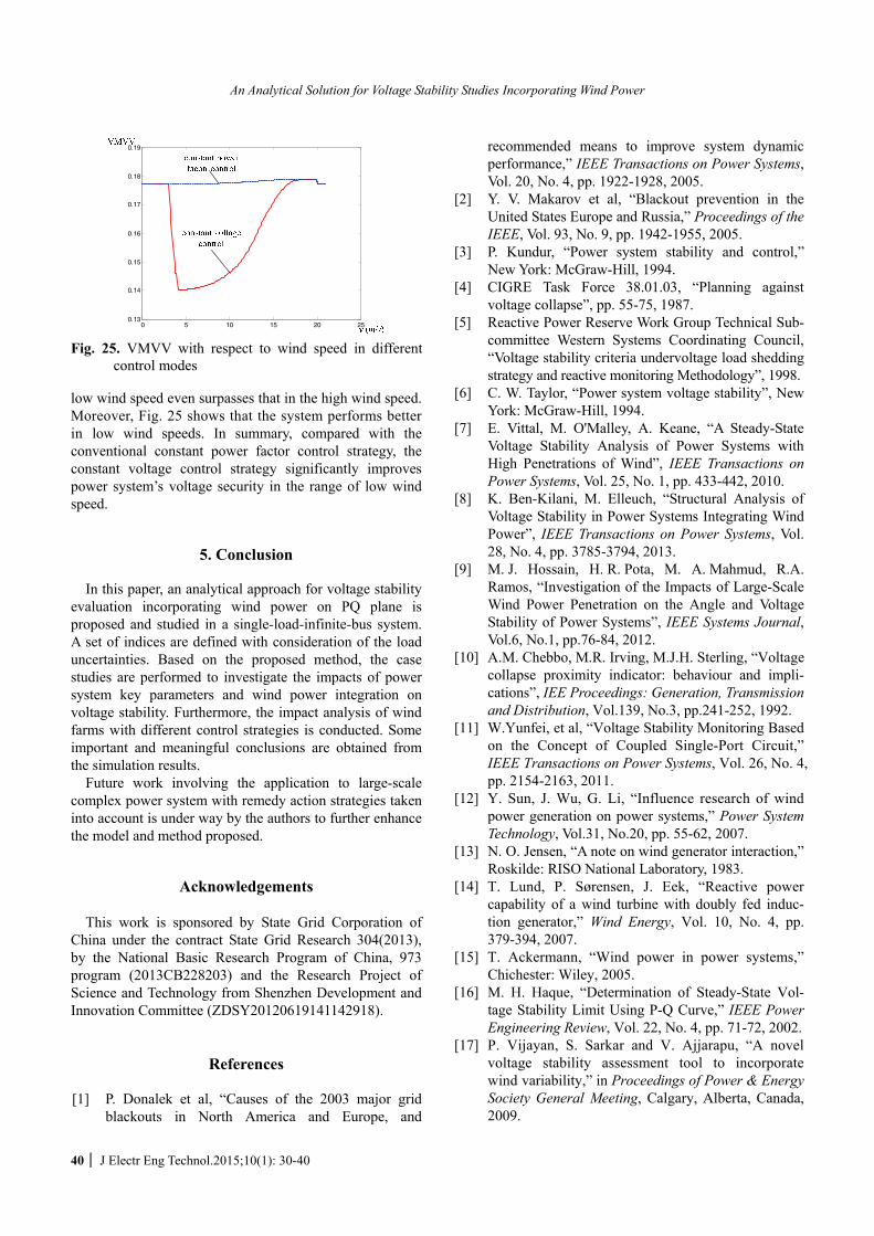
low wind speed even surpasses that in the high wind speed. Moreover, Fig. 25 shows that the system performs better in low wind speeds. In summary, compared with the conventional constant power factor control strategy, the constant voltage control strategy significantly improves power system’s voltage security in the range of low wind speed.

5. Conclusion In this paper, an analytical approach for voltage stability

evaluation incorporating wind power on PQ plane is proposed and studied in a single-load-infinite-bus system. A set of indices are defined with consideration of the load uncertainties. Based on the proposed method, the case studies are performed to investigate the impacts of power system key parameters and wind power integration on voltage stability. Furthermore, the impact analysis of wind farms with different control strategies is conducted. Some important and meaningful conclusions are obtained from the simulation results.

Future work involving the application to large-scale complex power system with remedy action strategies taken into account is under way by the authors to further enhance the model and method proposed.

Acknowledgements This work is sponsored by State Grid Corporation of

China under the contract State Grid Research 304(2013), by the National Basic Research Program of China, 973 program (2013CB228203) and the Research Project of Science and Technology from Shenzhen Development and Innovation Committee (ZDSY20120619141142918).

References

[1] P. Donalek et al, “Causes of the 2003 major grid blackouts in North America and Europe, and

recommended means to improve system dynamic performance,” IEEE Transactions on Power Systems, Vol. 20, No. 4, pp. 1922-1928, 2005.

[2] Y. V. Makarov et al, “Blackout prevention in the United States Europe and Russia,” Proceedings of the IEEE, Vol. 93, No. 9, pp. 1942-1955, 2005.

[3] P. Kundur, “Power system stability and control,” New York: McGraw-Hill, 1994.

[4] CIGRE Task Force 38.01.03, “Planning against voltage collapse”, pp. 55-75, 1987.

[5] Reactive Power Reserve Work Group Technical Sub-committee Western Systems Coordinating Council, “Voltage stability criteria undervoltage load shedding strategy and reactive monitoring Methodology”, 1998.

[6] C. W. Taylor, “Power system voltage stability”, New York: McGraw-Hill, 1994.

[7] E. Vittal, M. O'Malley, A. Keane, “A Steady-State Voltage Stability Analysis of Power Systems with High Penetrations of Wind”, IEEE Transactions on Power Systems, Vol. 25, No. 1, pp. 433-442, 2010.

[8] K. Ben-Kilani, M. Elleuch, “Structural Analysis of Voltage Stability in Power Systems Integrating Wind Power”, IEEE Transactions on Power Systems, Vol. 28, No. 4, pp. 3785-3794, 2013.

[9] M. J. Hossain, H. R. Pota, M. A. Mahmud, R.A. Ramos, “Investigation of the Impacts of Large-Scale Wind Power Penetration on the Angle and Voltage Stability of Power Systems”, IEEE Systems Journal, Vol.6, No.1, pp.76-84, 2012.

[10] A.M. Chebbo, M.R. Irving, M.J.H. Sterling, “Voltage collapse proximity indicator: behaviour and impli-cations”, IEE Proceedings: Generation, Transmission and Distribution, Vol.139, No.3, pp.241-252, 1992.

[11] W.Yunfei, et al, “Voltage Stability Monitoring Based on the Concept of Coupled Single-Port Circuit,” IEEE Transactions on Power Systems, Vol. 26, No. 4, pp. 2154-2163, 2011.

[12] Y. Sun, J. Wu, G. Li, “Influence research of wind power generation on power systems,” Power System Technology, Vol.31, No.20, pp. 55-62, 2007.

[13] N. O. Jensen, “A note on wind generator interaction,” Roskilde: RISO National Laboratory, 1983.

[14] T. Lund, P. Sørensen, J. Eek, “Reactive power capability of a wind turbine with doubly fed induc-tion generator,” Wind Energy, Vol. 10, No. 4, pp. 379-394, 2007.

[15] T. Ackermann, “Wind power in power systems,” Chichester: Wiley, 2005.

[16] M. H. Haque, “Determination of Steady-State Vol- tage Stability Limit Using P-Q Curve,” IEEE Power Engineering Review, Vol. 22, No. 4, pp. 71-72, 2002.

[17] P. Vijayan, S. Sarkar and V. Ajjarapu, “A novel voltage stability assessment tool to incorporate wind variability,” in Proceedings of Power & Energy Society General Meeting, Calgary, Alberta, Canada, 2009.

0 5 10 15 20 250.13

0.14

0.15

0.16

0.17

0.18

0.19

Fig. 25. VMVV with respect to wind speed in different

control modes



Yu-Zhang Lin He received B.S and M.S degrees in Electrical Engineering from Tsinghua University, China, in 2012 and 2014, respectively. His research interests are power system vulnerability analysis with voltage sta-bility constrained incorporating wind power.

Li-Bao Shi He received Ph.D. degree in Electrical Engineering from Chong-qing University, China, in 2000. His research interests are wind power in power systems, power system restora-tion control, computational intelligence in power system optimal operation and control, EMS/DMS, and power system

stability analysis.

Liang-Zhong Yao He received the PhD degree in 1993 in electrical power system engineering from Tsinghua University, China. He is currently the Vice President of State Grid Electric Power Research Institute, China. His research interests are wind power in power systems.

Yixin Ni She received her B. Eng., M. Eng. And Ph.D. degrees all from Tsinghua University, China. She was a former professor and director of National Power System Lab, Tsinghua Univ. and is currently with the Graduate School at Shenzhen, Tsinghua University. Her research interests are in

power system stability and control, HVDC transmission, FACTS, and power markets.

Shi-Yao Qin He received master degree in TaiYuan University of Sci-ence and Technology in 2003. His research interests are wind power simulation, planning, test technology.

Rui-Ming Wang He received master degree in North China Electric Power University in 2003. His research interests are wind power simulation, planning, test technology.

Jin-Ping Zhang He received master degree in HuaZhong University of Science and Technology in 2000. His research interests are wind farm and wind turbine test technology.

An Analytical Solution for Voltage Stability Studies ... · reactive power capability of wind...

Documents

Transcript of An Analytical Solution for Voltage Stability Studies ... · reactive power capability of wind...