An Analysis of the Perona-Malik Schemeesedoglu/Papers_Preprints/pm_esedoglu.pdf · An Analysis of...

An Analysis of the Perona-Malik Scheme

SELIM ESEDOGLUCourant Institute

Abstract

We investigate how the Perona-Malik scheme evolves piecewise smooth initialdata in one dimension. By scaling a natural parameter that appears in the schemein an appropriate way with respect to the grid size, we obtain a meaningful con-tinuum limit. The resulting evolution can be seen as the gradient flow for anenergy, just as the discrete evolutions are gradient flows for discrete energies.It involves, except at special isolated times, solving a system of heat equationscoupled to each other through nonlinear boundary conditions. At the specialtimes, the solutions experience gradient blowup; nevertheless, there is a naturalcontinuation for the solutions beyond these singular times.c© 2001 John Wiley& Sons, Inc.

1 Introduction

In [16] Perona and Malik proposed a numerical method for selectively smooth-ing digital images, designed to keep “edges” in pictures sharp. The essence of theirmethod is contained in the following discretization:

(1.1)ut+1t

i, j − uti, j

1t=

1

1x

(ct

Ei, j∇Eut

i, j − ctWi, j

∇Wuti, j

) + 1

1y

(ct

Ni, j∇Nut

i, j − ctSi, j

∇Suti, j

)whereN, S, E, andW denote north, south, east, and west, the symbol∇ denotesthe nearest-neighbor difference quotient in the direction of its subscript, and theremaining coefficients are given by

ctNi, j

= gk(|∇Nut

i, j |2), ct

Si, j= gk

(|∇Suti, j |2

),

ctEi, j

= gk(|∇Eut

i, j |2), ct

Wi, j= gk

(|∇Wuti, j |2

),

wheregk is a function with certain important properties, as we shall presently ex-plain. In applications, the computational domain is ordinarily just a rectangle, andone imposes either periodic or homogeneous Neumann boundary conditions.

In this paper we focus on the one-dimensional version of scheme (1.1). Ourpurpose is to recognize a continuum (PDE) problem that it solves in the limit asthe grid size1x goes to 0. As indicated, the functiongk comes equipped with a

Communications on Pure and Applied Mathematics, Vol. LIV, 0001–0046 (2001)c© 2001 John Wiley & Sons, Inc.

2 S. ESEDOGLU

parameterk; we obtain our continuum limit by choosing a specific relation betweenk and 1x. The resulting evolution is unusual: It involves solving a system ofheat equations coupled to each other through nonlinear boundary conditions thatbecome singular at special times, leading to gradient blowup for the solutions.However, the scheme suggests a natural continuation beyond each one of thesesingular times that involves a change in the PDE system. Our convergence proofapplies on any bounded interval of time, which might include singular times (undersome technical restrictions). And our continuum limit has some of the featuresobserved in applications of the numerical scheme.

It is natural to think of discretization (1.1) as a candidate for the numericalsolution of the continuum problem:

(1.2) ut = div(gk(|∇u|2)∇u) .

To be more precise, and as Perona and Malik note in their paper, the discretization(1.1) is suggestive of the similar but more anisotropic equation

(1.3) ut = (gk

(u2

x

)ux

)x+ (

gk

(u2

y

)uy

)y.

In fact, the authors propose their numerical scheme with this intention.An essential feature of the method is the choice of the functiongk(ξ). For

Perona and Malik’s choices, equation (1.2) (or (1.3)) is not parabolic: In regionsof high enough gradient (depending on the parameterk), the diffusion coefficientbecomes negative. Our approach avoids trying to make sense of equations (1.2) or(1.3). It instead concentrates on the scheme (1.1) itself.

1.1 Background

Image segmentation and edge detection are two fundamental procedures ofcomputer vision that rely on image smoothing as an important first step. Theirgoal is to decompose a given image into regions that are essentially homogeneous(with little variation in color or brightness). These regions should be separated bysharp boundaries (edges). Such an operation forms an early stage of interpretingand extracting useful information from digital pictures, since it helps recognizeparts of the scene that belong to different objects [14].

An image is described mathematically by a real-valued, bounded function de-fined on a subset of the plane; the value of the function at a point represents thegray-scale intensity, or brightness, at that point in the image. We think of edges inthe image as places where the intensity function has high gradient or discontinuitydue to an abrupt change. Abrupt changes in an image occur, however, not onlybecause of a transition from one distinct region in the scene to another, but alsobecause of the presence of noise or fine detail within regions. Those can appear asredundant edges. The natural approach of thresholding the gradient, therefore, isnot a satisfactory method of locating edges. As a cure, a preprocessing step is of-ten introduced. It involves smoothing the image—for instance, by some averagingtechnique—in order to remove noise and fine detail.

ANALYSIS OF PERONA-MALIK SCHEME 3

A common way of “de-noising” is to convolve the original image with theGauss kernel, or equivalently, to solve the heat equation with the original imageas initial data [12]. In that case, the variance of the kernel (or the time variablet of the heat equation) plays the role of a coarseness parameter. This method hasan obvious disadvantage: Edges in the image, which are the ultimate goal, getblurred. Ideally, ast gets large, we would like edges to remain sharp, and hencewell-defined and localized, until they disappear. One therefore wishes for a moreselective smoothing procedure: one that smoothes the interior of individual regionsbut not their boundaries.

Various methods have been suggested to avoid the disadvantages of Gauss-ian smoothing; a recurring theme is to replace the heat equation by a nonlineardiffusion equation. One such approach is directional diffusion, a typical example ofwhich is the equationut = |∇u| div(∇u/|∇u|) that models “motion by curvature”and also appears in other contexts [11]; it is degenerate along the gradient direction,and so has the effect of smoothing the image along but not across the edges. Peronaand Malik proposed another procedure in [16]. Their idea is to coarsen the imageusing a nonlinear heat equation whose constitutive function decreases rapidly forlarge values of the gradient and thus suppresses diffusion near edges. There are alsomethods based on modifications of Perona and Malik’s idea [2] and methods thatcombine their idea with the degeneracy in the motion by curvature equation [1].

1.2 The Perona-Malik MethodIn [16] Perona and Malik report numerical experiments with their scheme using

gk(ξ) = 1

1 + ξ

k

and gk(ξ) = exp

(− ξ

2k

).

Other choices used in practice include

gk(ξ) =(

1 + ξ

k

)(β−1)

whereβ ∈ (0, 1

2

).

These choices have the following common characteristics, as noted in [10]:

(1) gk(ξ) > 0 for all ξ ≥ 0.(2) The parameterk defines a positive critical valuez(k) such that∂ξ (ξgk(ξ

2))

> 0 for |ξ | < z(k) and∂ξ (ξgk(ξ2)) < 0 for |ξ | > z(k).

(3) Bothgk(ξ) and∂ξ (ξgk(ξ2)) tend to 0 asξ goes to infinity.

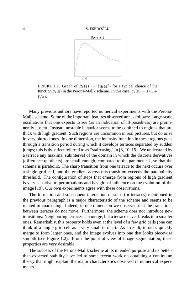
Figure 1.1 illustratesξgk(ξ2) for such a choice ofgk(ξ).

In light of these properties, the parameterk constitutes a threshold for the in-tensity gradient: In regions where the gradient is small compared tok, the equa-tion is parabolic. On the other hand, if the gradient is large compared tok, notonly does the diffusion coefficient vanish, but it actually becomes negative. Thisis an alarming situation since backwards heat equations are notoriously ill-posed.Nevertheless, experiments with the scheme yield visually impressive segmenta-tions [15, 16].

4 S. ESEDOGLU

z(k)

Rk(ξ) vs.ξ

FIGURE 1.1. Graph ofRk(ξ) := ξgk(ξ2) for a typical choice of the

functiongk(ξ) in the Perona-Malik scheme. In this case,gk(ξ) = 1/(1+ξ/k).

Many previous authors have reported numerical experiments with the Perona-Malik scheme. Some of the important features observed are as follows: Large-scaleoscillations that one expects to see (as an indication of ill-posedness) are promi-nently absent. Instead, unstable behavior seems to be confined to regions that arethick with high gradient. Such regions are uncommon in real pictures, but do arisein very blurred ones. In one dimension, the intensity function in these regions goesthrough a transition period during which it develops terraces separated by suddenjumps; this is the effect referred to as “staircasing” in [8, 10, 15]. We understand bya terrace any maximal subinterval of the domain in which the discrete derivatives(difference quotients) are small enough, compared to the parameterk, so that thescheme is parabolic. The sharp transition from one terrace to the next occurs overa single grid cell, and the gradient across this transition exceeds the parabolicitythreshold. The configuration of steps that emerge from regions of high gradientis very sensitive to perturbations and has global influence on the evolution of theimage [19]. Our own experiments agree with these observations.

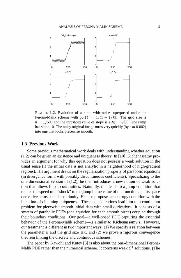
The formation and subsequent interaction of steps (or terraces) mentioned inthe previous paragraph is a major characteristic of the scheme and seems to berelated to coarsening. Indeed, in one dimension we observed that the transitionsbetween terraces do not move. Furthermore, the scheme does not introduce newtransitions: Neighboring terraces can merge, but a terrace never breaks into smallerones. Remarkably, this property holds even at the level of a few grid cells (one canthink of a single grid cell as a very small terrace). As a result, terraces quicklymerge to form larger ones, and the image evolves into one that looks piecewisesmooth (see Figure 1.2). From the point of view of image segmentation, theseproperties are very desirable.

The success of the Perona-Malik scheme at its intended purpose and its better-than-expected stability have led to some recent work on obtaining a continuumtheory that might explain the major characteristics observed in numerical experi-ments.


0 250 5000

1

2

3Original Image

0 250 5000

1

2

3t=0.002

0 250 5000

1

2

3t=0.02

0 250 5000

1

2

3t=0.04

FIGURE 1.2. Evolution of a ramp with noise superposed under thePerona-Malik scheme withgk(ξ) = 1/(1 + ξ/k). The grid size ish = 1/500 and the threshold value of slope isz(h) = √

80. The ramphas slope 10. The noisy original image turns very quickly (byt = 0.002)into one that looks piecewise smooth.

1.3 Previous Work

Some previous mathematical work deals with understanding whether equation(1.2) can be given an existence and uniqueness theory. In [10], Kichenassamy pro-vides an argument for why this equation does not possess a weak solution in theusual sense (if the initial data is not analytic in a neighborhood of high-gradientregions). His argument draws on the regularization property of parabolic equations(in divergence form, with possibly discontinuous coefficients). Specializing to theone-dimensional version of (1.2), he then introduces a new notion of weak solu-tion that allows for discontinuities. Naturally, this leads to a jump condition thatrelates the speed of a “shock” to the jump in the value of the function and its spacederivative across the discontinuity. He also proposes an entropy condition with theintention of obtaining uniqueness. These considerations lead him to a continuumproblem for piecewise smooth initial data with small derivatives. It consists of asystem of parabolic PDEs (one equation for each smooth piece) coupled throughtheir boundary conditions. Our goal—a well-posed PDE capturing the essentialbehavior of the Perona-Malik scheme—is similar to Kichenassamy’s. However,our treatment is different in two important ways: (1) We specify a relation betweenthe parameterk and the grid size1x, and (2) we prove a rigorous convergencetheorem linking the discrete and continuous schemes.

The paper by Kawohl and Kutev [8] is also about the one-dimensional Perona-Malik PDE rather than the numerical scheme. It concerns weakC1 solutions. (The

6 S. ESEDOGLU

set of such solutions is not empty, since if we start with initial data with smallslope, the equation remains parabolic for all time; such solutions therefore existand are well-behaved). Among the results presented is nonexistence of global-in-time weakC1 solutions whose initial data have regions with slope larger than theparabolicity threshold. So even for analytic initial data such solutions break downin finite time (if they exist at all; local-in-time existence is not known). Other re-sults the authors obtain include maximum and comparison principles and a unique-ness result for certainC1 solutions. Our continuum limit is rather different fromthat considered by Kawohl and Kutev. Still, we do make use of ideas from theirpaper in deriving a suitable maximum principle (Proposition 2.4).

In [3], Chambolle proves0-convergence of a class of discrete approximationsto the Mumford-Shah functional in two dimensions. Let us recall the form of thisfunctional:

(1.4) MS(u) :=∫

�−Su

|∇u|2 dx + αH1(Su) + λ

∫�

|u − u0|2 dx .

It is defined for functionsu in GSBV, the space of generalized special functionsof bounded variation.H1 denotes the one-dimensional Hausdorff measure,Su isthe jump set ofu and∇u its approximate gradient, andu0 is the original image.Chambolle’s approximations to MS, withH1 replaced by an anisotropic version(cab driver length), are defined on uniform rectangular grids; they look like

Eh(u) :=∑i, j

h2

{Wk

(ui+1, j − ui, j

h

)+ Wk

(ui, j +1 − ui, j

h

)}

+ λ∑i, j

h2|ui, j − u0i, j |2

where the functionWk(x) := min{x2, k} andh > 0 is the grid size. The functionWk is convex for|x| ≤ √

k. In that sense, the parameterk plays the same kindof thresholding role as it does in the Perona-Malik scheme. Chambolle shows thatif k is scaled ask = α/h with respect to the grid size, this family of discretefunctionals0-converge to MS. The Perona-Malik method is dynamic, while theMumford-Shah variational problem is static. There is, however, a very strong linkbetween our work and that of Chambolle: We follow his lead in assuming that theparameterk must scale withh.

Paper [6] by Gobbino concerns the same kind of problem with a similar ap-proach as in Chambolle’s work. It establishes0-convergence to MS (withλ = 0,an inessential difference) of a class of approximations that in one dimension havethe form

(1.5) Fε(u) := 1

ε

∫R

arctan

((u(x + ε) − u(x))2

ε

)dx .

Gobbino’s result in fact holds for then-dimensional analogue of the problem.


The more recent paper by Gobbino [7] is dynamic rather than static and veryclosely related to the present work. This paper looks at the one-dimensional ap-proximations (1.5) as defined on spaces of piecewise constant functions

PC2ε :=

{u ∈ L2(R) : u(x) = u

(ε

[x

ε

]),∀x ∈ R

}

whereε > 0 is the grid size and[·] denotes the integer part of its argument. Thepaper is devoted to defining a gradient flow for MS as the limit of gradient flows to(1.5), which are defined by the relation

(1.6) u′ε(x) = −(∇Fε)(uε(t)) with uε(0) = u0

ε .

The initial conditionu0 is required to beL∞loc and have finite Mumford-Shah energy.

In one dimension, this stipulation implies thatu0 is piecewiseW1,2. Also, theapproximate initial datau0

ε (which are piecewise constant) must converge tou0

in L2 and in energy. Gobbino shows that the flows generated by (1.6) converge,and for a large class of initial data the limit is independent of the approximatingsequence.

Gobbino’s paper is related to our work because the gradient flows (1.5) aregiven precisely by the semidiscrete (continuous-in-time) version of the Perona-Malik scheme (1.1) withgk(ξ) = 1/(1 + ξ2/k2) and subject to the scalingk =1/1x. The limiting evolution he obtains is similar to ours, consisting of solving asystem of linear heat equations in a variable domain. However, it differs from oursin the boundary conditions that couple these equations to each other: His equationshave a homogeneous Neumann boundary condition at each “interface,” whereasour limit involves nonlinear boundary conditions that strongly couple equationson neighboring intervals to each other. Our analysis is therefore similar to that ofGobbino at many points but also requires new ideas.

1.4 Our Approach

We now turn to the central task of this paper: understanding the Perona-Malikscheme (1.1) as the grid sizeh goes to 0 withk = k(h) scaled appropriately. Weshall address the semidiscrete version of the scheme (discrete in space, continuousin time), and we restrict our attention to one space dimension. Thus, the scheme tobe analyzed is

(1.7)d

dtuj (t) = 1

h

(Rk(∇Euj (t)) − Rk(∇Wuj (t))

)whereRk(ξ) := ξgk(ξ

2). We will work with the specific family of nonlinearities

gβ,k(ξ) =(

1 + ξ

k

)(β−1)

with β ∈ [0, 1

2

).

8 S. ESEDOGLU

Let z(h) = zβ(h) denote the threshold value of the slope for this family; moreexplicitly,

z(h) = 1√1 − 2β

√k(h)

so that

∂ξ Rβ,h(ξ)

{> 0 for |ξ | < z(h)

≤ 0 otherwise.

For later reference, we record two important properties of the functionR. First,R(ξ) := Rk(ξ) is a one-to-one, increasing function on[−z(h), z(h)]; it thereforehas an increasing inverse with domain[−R(z(h)), R(z(h))]. We shall denote thisfunction R−1∗ , i.e.,

(1.8) R−1∗ (ξ) := (

R(ξ)∣∣[−z(h),z(h)]

)−1.

Second, sinceRh(x)/x is a function of onlyx/z, we have the following boundfrom below, which is independent ofh:

(1.9) θ(β) := inf|x|<z(h)/2|y|<z(h)

∣∣∣∣ Rh(x) − Rh(y)

x − y

∣∣∣∣ > 0 .

Let us now try to understand how the one-dimensional scheme (1.7) operateson an initial image that is smooth except at a pointp, at which it has a jump ofheight J. Let p be located between the two grid pointsxj andxj +1. The schemethen reads

uj = 1

h

(Rk

(J

h

) − Rk

(uj − uj −1

h

)),

uj +1 = 1

h

(Rk

(uj +2 − uj +1

h

)− Rk

(J

h

)).

Roughly speaking, we interpret this to mean that the scheme imposes the condition

(1.10) Rk

(uj − uj −1

h

)= Rk

(J

h

)= Rk

(uj +2 − uj +1

h

).

In words, the slopes on either side of a jump are equal and are related to the jumpheight by the above formula. One way to understand why this is so is to note thatunless these three quantities are withinO(h) of each other, a process that operatesat a faster time scale will adjust them until this is the case. Kichenassamy alsoobserved this property as a “note added in proof” of his paper [10].

We therefore expect the scheme to impose (possibly inhomogeneous) Neumannboundary conditions at jump locations of a piecewise smooth image.

Second, we note that the difference quotients(uj +1 − uj )/h scale asO(1) atdifferentiable regions in the image and asO(1/h) across jumps. We are thus ledto look for a way to adjust the thresholding parameterk that appears in the schemewith respect to grid sizeh so that relation (1.10) translates into a nontrivial bound-ary condition in the limit ash → 0+.


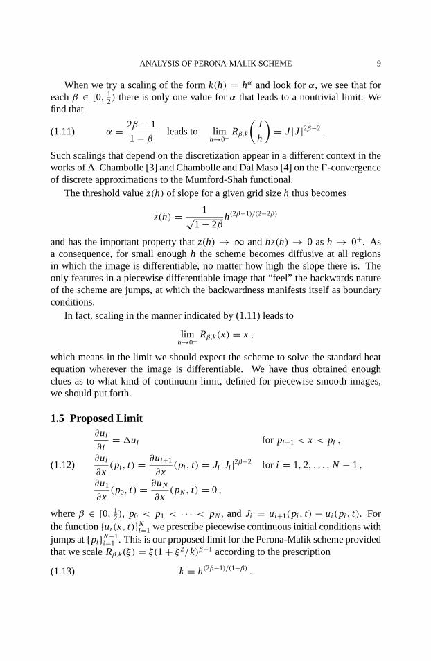
When we try a scaling of the formk(h) = hα and look forα, we see that foreachβ ∈ [0, 1

2) there is only one value forα that leads to a nontrivial limit: Wefind that

(1.11) α = 2β − 1

1 − βleads to lim

h→0+ Rβ,k

(J

h

)= J|J|2β−2 .

Such scalings that depend on the discretization appear in a different context in theworks of A. Chambolle [3] and Chambolle and Dal Maso [4] on the0-convergenceof discrete approximations to the Mumford-Shah functional.

The threshold valuez(h) of slope for a given grid sizeh thus becomes

z(h) = 1√1 − 2β

h(2β−1)/(2−2β)

and has the important property thatz(h) → ∞ andhz(h) → 0 ash → 0+. Asa consequence, for small enoughh the scheme becomes diffusive at all regionsin which the image is differentiable, no matter how high the slope there is. Theonly features in a piecewise differentiable image that “feel” the backwards natureof the scheme are jumps, at which the backwardness manifests itself as boundaryconditions.

In fact, scaling in the manner indicated by (1.11) leads to

limh→0+ Rβ,k(x) = x ,

which means in the limit we should expect the scheme to solve the standard heatequation wherever the image is differentiable. We have thus obtained enoughclues as to what kind of continuum limit, defined for piecewise smooth images,we should put forth.

1.5 Proposed Limit∂ui

∂t= 1ui for pi−1 < x < pi ,

∂ui

∂x(pi , t) = ∂ui+1

∂x(pi , t) = Ji |Ji |2β−2 for i = 1, 2, . . . , N − 1 ,(1.12)

∂u1

∂x(p0, t) = ∂uN

∂x(pN, t) = 0 ,

whereβ ∈ [0, 12), p0 < p1 < · · · < pN , and Ji = ui+1(pi , t) − ui (pi , t). For

the function{ui (x, t)}Ni=1 we prescribe piecewise continuous initial conditions with

jumps at{pi }N−1i=1 . This is our proposed limit for the Perona-Malik scheme provided

that we scaleRβ,k(ξ) = ξ(1 + ξ2/k)β−1 according to the prescription

(1.13) k = h(2β−1)/(1−β) .

10 S. ESEDOGLU

0 0.5 1

−0.5

0

0.5

Original Image

0 0.5 1

−0.5

0

0.5

t=0.04

0 0.5 1

−0.5

0

0.5

t=0.049

0 0.5 1

−0.5

0

0.5

t=0.059

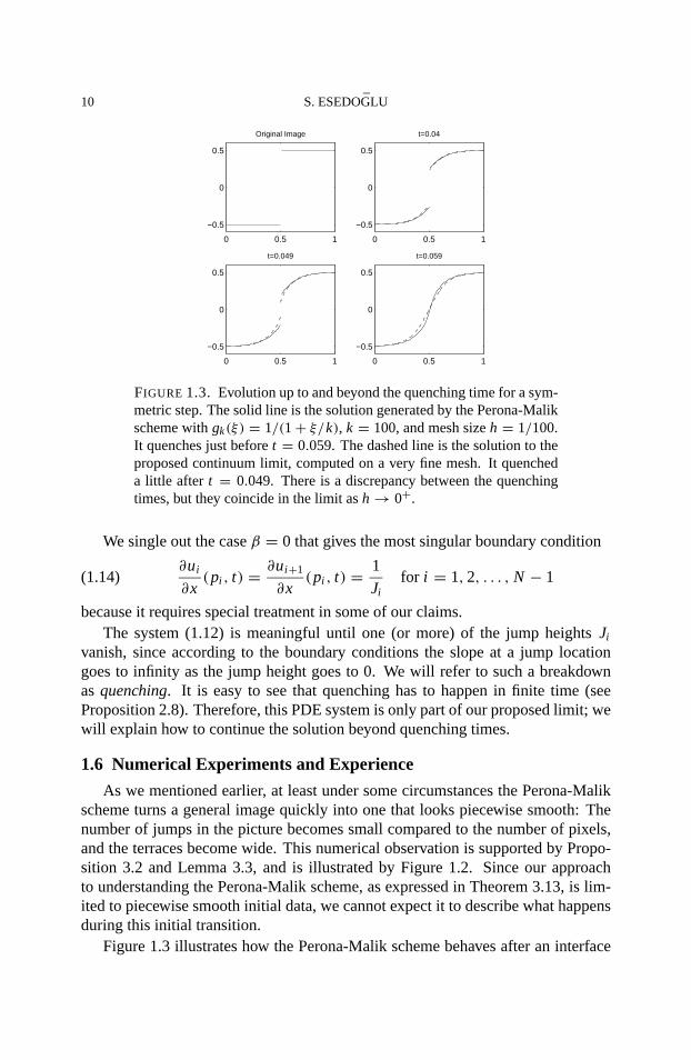
FIGURE 1.3. Evolution up to and beyond the quenching time for a sym-metric step. The solid line is the solution generated by the Perona-Malikscheme withgk(ξ) = 1/(1 + ξ/k), k = 100, and mesh sizeh = 1/100.It quenches just beforet = 0.059. The dashed line is the solution to theproposed continuum limit, computed on a very fine mesh. It quencheda little after t = 0.049. There is a discrepancy between the quenchingtimes, but they coincide in the limit ash → 0+.

We single out the caseβ = 0 that gives the most singular boundary condition

(1.14)∂ui

∂x(pi , t) = ∂ui+1

∂x(pi , t) = 1

Jifor i = 1, 2, . . . , N − 1

because it requires special treatment in some of our claims.The system (1.12) is meaningful until one (or more) of the jump heightsJi

vanish, since according to the boundary conditions the slope at a jump locationgoes to infinity as the jump height goes to 0. We will refer to such a breakdownasquenching. It is easy to see that quenching has to happen in finite time (seeProposition 2.8). Therefore, this PDE system is only part of our proposed limit; wewill explain how to continue the solution beyond quenching times.

1.6 Numerical Experiments and Experience

As we mentioned earlier, at least under some circumstances the Perona-Malikscheme turns a general image quickly into one that looks piecewise smooth: Thenumber of jumps in the picture becomes small compared to the number of pixels,and the terraces become wide. This numerical observation is supported by Propo-sition 3.2 and Lemma 3.3, and is illustrated by Figure 1.2. Since our approachto understanding the Perona-Malik scheme, as expressed in Theorem 3.13, is lim-ited to piecewise smooth initial data, we cannot expect it to describe what happensduring this initial transition.

Figure 1.3 illustrates how the Perona-Malik scheme behaves after an interface


0 250 5000

1

2

3Original Image

0 250 5000

1

2

3t=0.005

0 250 5000

1

2

3t=0.02

0 250 5000

1

2

3t=0.04

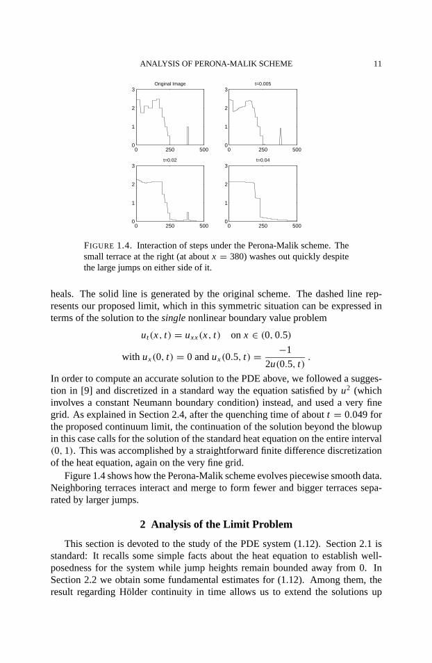
FIGURE 1.4. Interaction of steps under the Perona-Malik scheme. Thesmall terrace at the right (at aboutx = 380) washes out quickly despitethe large jumps on either side of it.

heals. The solid line is generated by the original scheme. The dashed line rep-resents our proposed limit, which in this symmetric situation can be expressed interms of the solution to thesinglenonlinear boundary value problem

ut(x, t) = uxx(x, t) on x ∈ (0, 0.5)

with ux(0, t) = 0 andux(0.5, t) = −1

2u(0.5, t).

In order to compute an accurate solution to the PDE above, we followed a sugges-tion in [9] and discretized in a standard way the equation satisfied byu2 (whichinvolves a constant Neumann boundary condition) instead, and used a very finegrid. As explained in Section 2.4, after the quenching time of aboutt = 0.049 forthe proposed continuum limit, the continuation of the solution beyond the blowupin this case calls for the solution of the standard heat equation on the entire interval(0, 1). This was accomplished by a straightforward finite difference discretizationof the heat equation, again on the very fine grid.

Figure 1.4 shows how the Perona-Malik scheme evolves piecewise smooth data.Neighboring terraces interact and merge to form fewer and bigger terraces sepa-rated by larger jumps.

2 Analysis of the Limit Problem

This section is devoted to the study of the PDE system (1.12). Section 2.1 isstandard: It recalls some simple facts about the heat equation to establish well-posedness for the system while jump heights remain bounded away from 0. InSection 2.2 we obtain some fundamental estimates for (1.12). Among them, theresult regarding Hölder continuity in time allows us to extend the solutions up

12 S. ESEDOGLU

to the singular (quenching) times. That paves the way to Section 2.4, where weexplain how to modify the PDE system and continue the solution after an interfaceheals. In Section 2.3 we look more carefully into what happens in a neighborhoodof quenching times. Our results show that the solutions do not spend too muchtime with large gradients: Under suitable conditions, quenching time for a jumpcan be estimated from above in terms of the jump height.

The results we obtain here have discrete analogues for the Perona-Malik schemeand will be derived also in that context in Section 3. Together, they will eventuallybe used in our convergence argument.

2.1 Existence, Uniqueness, and Regularity

We first consider the following linear Neumann problem on an interval:Given continuous and boundedf (t) andg(t) and continuous

φ(x) : [pi−1, pi ] → R ,

find u ∈ C2,1([pi−1, pi ] × (0,∞)) ∩ C([pi−1, pi ] × [0,∞)) such that

ut(x, t) = uxx(x, t) on x ∈ (pi−1, pi ) for t > 0 ,

ux(pi−1, t) = f (t) and ux(pi , t) = g(t) for t > 0 ,(2.1)

u(x, 0) = φ(x) .

The solution to this problem can be represented via the method of images, asfollows: Let

P(x, y, t) =∞∑

n=−∞

1√2π t

{e−(x−y−2n)2/(2t) + e−(x+y−2n)2/(2t)

},

Pi (x, y, t) = 1

pi − pi−1P

(x − pi−1

pi − pi−1,

y − pi−1

pi − pi−1,

t

(pi − pi−1)2

).

Then the solution to problem (2.1) is given by

u(x, t) =∫ t

0Pi (x, pi−1, t − s) f (s)ds+

∫ t

0Pi (x, pi , t − s)g(s)ds

+∫ pi

pi −1

Pi (x, y, t)φ(y)dy .

(2.2)

Some Basic Estimates

From the explicit formula (2.2) we can compute various derivatives of the solu-tion. That yields estimates such as the following:

(2.3) supx∈[pi −1,pi ]

T≥t≥ε

∑2α+β≤2nα,β∈N

|Dαt Dβ

x u(x, t)| ≤ C(ε, T){| f |Cn

ε,T+ |g|Cn

ε,T+ |φ|L1

}


where| f |Cnε,T

:= | f |Cn([ε,T]). If we also restrictx to remain bounded away fromthe spatial boundary, we can bound interior derivatives by low-order norms off ,g, andφ:

(2.4) supx∈[pi −1+δ,pi −δ]

T≥t≥ε

|Dαt Dβ

x u(x, t)| ≤ C(ε, δ, T){| f |L∞ + |g|L∞ + |φ|L1

}.

The case of the firstx-derivativeux(x, t) is slightly better in that for positive timeit is controlled by the lower norms up to the spatial boundary

(2.5) supx∈[pi −1,pi ]

T≥t≥ε

|ux(x, t)| ≤ C(ε, T){| f |L∞ + |g|L∞ + |φ|L1

}.

Solution of the Nonlinear System

We establish local-in-time existence and uniqueness for continuous initial data.

PROPOSITION2.1 The system of equations

(2.6)

∂ui

∂t= ∂2ui

∂x2for pi−1 < x < pi ,

∂ui

∂x(pi , t) = ∂ui+1

∂x(pi , t)

= fi (ui+1(pi , t) − ui (pi , t)) for i 6= 0, N ,

∂u1

∂x(p0, t) = ∂uN

∂x(pN, t) = 0 ,

ui (x, 0) = φi (x) ,

where the fi (x) are Lipschitz-continuous and the functionsφi (x) in the initial con-dition are continuous, has a unique(local-in-time) solution.

PROOF: Let Xi = {u ∈ C([0, T]× Ii ) : u(x, 0) = φi (x)} with Ii := (pi−1, pi ),and setX = X1 × X2 × · · · × XN . On this set we take the metric

d(u, v) := maxi=1,2,...,N

supx∈Ii

t∈[0,T]|ui (x, t) − vi (x, t)| for u, v ∈ X.

14 S. ESEDOGLU

Now consider the mappingS : X → X defined in the following manner: Forv ∈ X, S(v) = u whereui is the solution of the problem:

∂ui

∂t= ∂2ui

∂x2in Ii ,

∂ui

∂x(pi , t) = ∂ui+1

∂x(pi , t) = fi (vi+1(pi , t) − vi (pi , t)) for i 6= 0, N ,

∂u1

∂x(p0, t) = ∂uN

∂x(pN, t) = 0 ,

ui (x, 0) = φi (x) ,

which is a linear decoupled system whose solutions can be expressed by formula(2.2). Indeed, if we letJi [u](t) := ui+1(pi , t) − ui (pi , t), we obtain the formula

S(u)i =∫ pi

pi −1

Pi (x, y, t)φ(y)dy +∑

j =i−1,i

∫ t

0Pi (x, pj , s) f j (Jj [u](t − s))ds.

We will show that the mappingS can be made contractive by choosingT > 0small enough. To this end, letu, v ∈ X and setL := maxi Lip( fi ). Then therepresentation obtained above implies

|S(u)i − S(v)i | ≤ L∫ t

0Pi (x, pi−1, t − s)|ui−1(pi−1, s) − vi−1(pi−1, s)|ds

+ L∫ t

0Pi (x, pi−1, t − s)|ui (pi−1, s) − vi (pi−1, s)|ds

+ L∫ t

0Pi (x, pi , t − s)|ui (pi , s) − vi (pi , s)|ds

+ L∫ t

0Pi (x, pi , t − s)|ui+1(pi , s) − vi+1(pi , s)|ds,

which by the elementary bound∣∣∣∣∫ t

0Pi (x, y, t − s)ds

∣∣∣∣ ≤ C√

t

implies the inequality

suppi −1≤x≤pi

0≤t≤T

|S(u)i − S(v)i | ≤ C√

T d(u, v)

whereC depends onL. But then taking the maximum overi we get

d(S(u), S(v)) ≤ C√

T d(u, v) ,

which of course means we have a contraction for a sufficiently small choice ofT > 0. It follows that the mappingS has a fixed pointu(x, t) in the (complete)metric spaceX. This is our candidate for the solution to the system.


Next, we note thatu(x, t) can be recognized as the limit of a sequence{u(n)}∞n=0

whereu(0)i (x, t) := φi (x) andu(n+1)(x, t) := S(u(n)) for n = 0, 1, . . . , by def-

inition. By virtue of our argument, this sequence converges uniformly as soonas we ensure thatS is contractive by takingT > 0 suitably small. Applyingestimate (2.4) tou(n)(x, t) − u(m)(x, t), we see that the sequence of derivatives{Dα

t Dβx u(n)(x, t)}∞n=1 converges uniformly on every compactly included subset of

(p0, p1)×(p1, p2)×· · ·×(pN−1, pN)×(0, T), and therefore the limiting functionu(x, t) is smooth on this domain and satisfies the heat equation there just like everyterm in the sequence.

We also need to check that the boundary condition makes sense (i.e., the limitpossesses one derivative inx up to the boundary for positive time) and is satis-fied. This is a consequence of (2.5) applied once again tou(n)(x, t) − u(m)(x, t);this time we see that{u(n)

x (x, t)}∞n=1 converges uniformly on every set of the form[p0, p1] × [p1, p2] × · · · × [pN−1, pN] × [ε, T − ε]. So the limitu(x, t) possessesanx-derivative up to the spatial boundary, and since the sequence of boundary val-ues{ f j (u(n)(pj +1, t))− f j (u(n)(pj , t))}∞n=1 converge tof j (u(pj +1, t)−u(pj , t)), itsatisfies the correct boundary condition.

Finally, the candidateu(x, t) assumes the correct initial value ast → 0+ asa consequence of its continuity and the manner in which the sequence has beenconstructed. We hence see thatu(x, t) is the unique solution of the nonlinear sys-tem. �Remark.The choice ofT > 0 in the existence argument is constrained only by thesize of the Lipschitz constants of the functionsfi . Therefore, in case the functionsare globally Lipschitz, by iteration of the argument we can obtain global-in-timeexistence.

Higher Regularity

We need bounds on higher derivatives (e.g.,uxxx) on the domain[p0, p1] ×[p1, p2]× · · · × [pN−1, pN]× (0, T); in other words, we need higher regularity upto the spatial boundary for positive time. This will be needed for the convergenceargument later on, where we shall need to estimate how well difference quotientsapproximate first and second derivatives of the solution to the system.

PROPOSITION2.2 Let f1, f2, . . . , fN−1 ∈ C∞, and let u(x, t) = {ui (x, t)}Ni=1 be

the solution to the system with nonlinear boundary conditions(2.6). Then

ui (x, t) ∈ C∞([pi−1, pi ] × (0,∞)) for i = 1, 2, . . . , N .

PROOF: We recall some fundamental properties of heat potentials; for details,see [5] and [13]. First, iffi (t) are continuous functions, then the single layerpotential

(2.7)∑

j =i−1,i

∫ t

0Pi (x, pj , s) f j (s)ds

16 S. ESEDOGLU

is Cγ,γ /2([pi−1, pi ] × [δ, T − δ]) for anyγ ∈ (0, 12). To fix ideas, takeγ = 1

4. It iseasy to see by a uniqueness argument that this impliesu(x, t) has the same Höldercontinuity.

Second, iffi (t) ∈ Cν/2 whereν is a noninteger positive number, then the single-layer potential given in (2.7) is in factCν+1,(ν+1)/2. In other words, convolutionwith the heat potentialPi as in (2.7) allows us to gain (at least) one full derivativein thex-direction and half a derivative (in the Hölder sense) in thet-direction.

The proof of regularity can now proceed by induction. Assumeu ∈ Cγ,γ /2 sothat u(pi , t) areCγ /2-functions of time. Then the jump heightsJi [u](t) ∈ Cγ /2.Since the functionsfi areC∞, we get

∂xui (pi , t) = ∂xui+1(pi , t) = fi (Ji [u](t)) ∈ Cγ /2 .

Our remarks in the previous paragraph implyui (x, t) ∈ Cγ+1,(γ+1)/2. By induc-tion, u ∈ C∞. �

COROLLARY 2.3 System(1.12), proposed as a continuum limit for the Perona-Malik scheme, has a unique solution with good regularity properties while the jumpheights Ji (t) remain bounded away from0.

PROOF: In terms of the notation employed in the existence proof, the proposedcontinuum limit (1.12) is nothing other than system (2.6) withfi (ξ) := ξ |ξ |2β−2

for i = 1, 2, . . . , N − 1.Let m := mini=1,2,...,N−1 Ji (0) > 0, and fixε ∈ (0, m). Let f (ε)(ξ) be aC∞-

function such thatf (ε)(ξ) = ξ |ξ |2β−2 for |ξ | > ε. Apply the existence theorem(2.1) with the choice of functionsfi (ξ) = f (ε)(ξ) for i = 1, 2, . . . , N − 1. Thatyields a (global-in-time) solution; call itu(ε)(x, t). But thenu(ε)(x, t) is a solutionto the system (1.12) as long as mini=1,2,...,N−1 u(ε)

i+1(pi , t) − u(ε)i (pi , t) ≥ ε. Note

that if 0 < ε′ < ε, thenu(ε) = u(ε′) while mini u(ε′)i+1(pi , t) − u(ε′)

i (pi , t) ≥ ε. Thatproves our claim, sinceε > 0 can be chosen arbitrarily small. �

2.2 Properties of Solutions

Here we discuss some important properties of solutions to the proposed con-tinuum limit: maximum principle, bounds on gradients, and Hölder continuity intime. We will denoteu(x, t) the piecewise continuous function on[p0, pN] whereu(x, t) := ui (x, t) for x ∈ (pi−1, pi ).

PROPOSITION2.4 (Maximum Principle)Let u(x, t) := {ui (x, t)}Ni=1 be a solution

to the proposed continuum limit(1.12)for 0 ≤ t ≤ T withβ ∈ [0, 12). Then for all

t ≥ 0,

supx

|u(x, t)| ≤ supx

|u(x, 0)| .


PROOF: A convenient way of showing this statement is to follow an argumentgiven in [8]. Set f (ξ) = ξ |ξ |2β−2, the boundary conditions in (1.12). Then

1

p

d

dt

∫ pi

pi −1

|ui |p dx =∫ pi

pi −1

|ui |p−2ui ∂2xui dx

≤ |ui |p−2ui ∂xui

∣∣∣pi

pi −1

= |ui |p−2ui f (ui+1 − ui )

∣∣∣pi

− |ui |p−2ui f (ui − ui−1)

∣∣∣pi −1

.

Summing overi = 1, 2, . . . , N we see that

1

p

d

dt

N∑i=1

∫ pi

pi −1

|ui |p dx ≤N−1∑i=1

[|ui |p−2ui − |ui+1|p−2ui+1]

f (ui+1 − ui )

∣∣∣pi

,

which is negative becausex f (x) ≥ 0 for our specific choice of boundary condi-tions, and

(|x|p−2x − |y|p−2y)(x − y) ≥ 0

for all x, y provided thatp > 1. Letting p → ∞ gives the desired result. �

For ε > 0 andp > 1 let

Fp,ε(x) = (x2 + ε2)p/2

so that

(2.8) F ′′p,ε(x) ≥

{0 for all p > 1

p(p − 1)(x2 + ε2)(p−2)/2 for p ∈ (1, 2] .

Now we compute

d

dt

N∑i=1

∫ pi

pi −1

Fp,ε(∂xui )dx

=N∑

i=1

∫ pi

pi −1

F ′p,ε(∂xui )∂xtui dx

= −N∑

i=1

∫ pi

pi −1

F ′′p,ε(∂xui )∂

2xui ∂tui dx +

N∑i=1

F ′p,ε(∂xui )∂tui

∣∣∣pi

pi −1

where we integrated by parts in the last step. Invoking the boundary conditions(1.12), we find

d

dt

N∑i=1

∫ pi

pi −1

Fp,ε(∂xui )dx = −N∑

i=1

∫ pi

pi −1


2xui ∂tui dx

−N∑

i=1

F ′p,ε(Ji (t)|Ji (t)|2β−2)∂t Ji (t)

(2.9)

18 S. ESEDOGLU

where we rearranged the terms in the last sum. Integrating int over (t1, t2) andmaking the change of variabley = Ji (t) in the boundary terms that make up thelast sum, we obtain the equation

N∑i=1

∫ pi

pi −1

Fp,ε(∂xui )dx∣∣∣t2t1

= −N∑

i=1

∫ t2

t1

∫ pi

pi −1


2xui ∂tui dx dt

−N−1∑i=1

∫ Ji (t2)

Ji (t1)F ′

p,ε(y|y|2β−2)dy .

(2.10)

From this formula we obtain the following estimates:

PROPOSITION2.5 (L p-Bound for Derivatives)Let u(x, t) = {ui (x, t)}∞i=1 be asolution to system(1.12)with β ∈ [0, 1

2) for 0 ≤ t < T . We then have

sup0<t≤T

N∑i=1

∫ pi

pi −1

∣∣∣∣∂ui

∂x(x, t)

∣∣∣∣p

dx = C(p) < ∞

where1 < p < 2(1− β)/(1− 2β). Furthermore, the constant C(p) depends onlyon the piecewise W1,p-norm of the initial condition and the initial jump heights, inaddition to p andβ.

PROOF: Since∂tui = ∂2xui andF ′′

p,ε(ξ) ≥ 0 for all ξ as seen in (2.8), we get


2xui ∂tui = F ′′

p,ε(∂xui )(∂tui )2 ≥ 0 .

So the first term in the right-hand side of formula (2.10) is negative; once we letε

go to 0 in this formula, we therefore get the inequality

N∑i=1

‖∂xui (·, t2)‖pL p(pi −1,pi )

≤N∑

i=1

‖∂xui (·, t1)‖pL p(pi −1,pi )

+ pN−1∑i=1

∫ Ji (t2)

Ji (t1)|y|(2β−1)(p−1) dy

The integrands on the right-hand side are locally integrable forp < 2(1−β)/(1−2β). Furthermore, the intervals of integration can be bounded in terms of the initialcondition by using, for example, Proposition 2.4 (the maximum principle). Thatproves the claim, since the right-hand side is shown to be controlled completely interms of the initial condition. �

A most important property of solutions to the proposed limit (1.12) with theless singular boundary conditions that correspond toβ ∈ (0, 1

2) is that they are thesteepest descent for an energy. This is merely a special case of equation (2.9):


PROPOSITION2.6 (Steepest Descent)Let u(x, t) = {ui (x, t)}Ni=1 be a solution to

system(1.12)with β ∈ (0, 12) for 0 ≤ t < T . Define the energy

(2.11) Eu(t) := 1

2

N∑i=1

∫ pi

pi −1

(∂ui

∂x(x, t)

)2

dx + 1

2β

N−1∑i=1

|Ji (t)|2β .

Then the following relation holds:

(2.12)d

dtEu(t) = −

N∑i=1

∫ pi

pi −1

(∂ui

∂t(x, t)

)2

dx .

PROOF: In equation (2.9) takep = 2 andε = 0. Noting that

d

dt

1

2β|Ji (t)|2β = F2,0

(Ji (t)|Ji (t)|2β−2

),

we obtain the promised formula. �

Remark.The caseβ = 0 decreases the energy

Eu(t) := 1

2

N∑i=1

∫ pi

pi −1

(∂ui

∂x(x, t)

)2

dx +N−1∑i=1

log(|Ji (t)|) ,

which, however, is not bounded from below asJi → 0.

As a consequence of the estimates above, we obtain the following Hölder-continuity-in-time result, which shows that solutions to the continuum limit evolveslowly all the way up to the singular times.

COROLLARY 2.7 (Hölder Continuity)Let u(x, t) = {ui (x, t)}∞i=1 be a solution tosystem(1.12)with β ∈ (0, 1

2) for 0 ≤ t < T . Then for i= 1, 2, . . . , N,

ui (t, ·) ∈ C1/2([0, T); L2((pi−1, pi ))

)and

ui (t, ·) ∈ C1/4([0, T); L∞((pi−1, pi ))

).

For the more singular caseβ = 0, we instead have

ui (t, ·) ∈ Cµ([0, T); L2((pi−1, pi ))

)and

ui (t, ·) ∈ Cν([0, T); L∞((pi−1, pi ))

)for anyµ ∈ (0, 1

2) andν ∈ (0, 14). Furthermore, in all cases the Hölder constants

involved depend only on the appropriate piecewise W1,p-norm and jump heightsof the initial condition.

20 S. ESEDOGLU

PROOF: By an application of the Hölder inequality followed by switching theorder of integration, we have

N∑i=1

∫ pi

pi −1

|ui (x, t2) − ui (x, t1)|2 dx =N∑

i=1

∫ pi

pi −1

∣∣∣∣∫ t2

t1

∂ui

∂t(x, s)ds

∣∣∣∣2

dx

≤ |t2 − t1|N∑

i=1

∫ t2

t1

∫ pi

pi −1

∣∣∣∣∂ui

∂t(x, s)

∣∣∣∣2

dx ds.

The right-hand side of the above inequality can now be bounded by the integral int over[t1, t2] of the energy identity (2.12) to get

N∑i=1

∫ pi

pi −1

∣∣ui (x, t2) − ui (x, t1)∣∣2

dx ≤ |t2 − t1|(Eu(t1) − Eu(t2)

)≤ |t2 − t1|Eu(t1) ,

which is exactly the definition ofC1/2 Hölder continuity in time with values inL2

of space, and the Hölder constant(Eu(t1))1/2 depends on conditions at the begin-ning of the time interval, as promised.

To get Hölder continuity with values inL∞ of space, first note that by Proposi-tion 2.5 theL2-norm of derivatives∂xui are bounded:

supt≥0

N∑i=1

‖∂xui (·, t)‖L p((pi −1,pi )) < ∞ .

We can therefore apply the interpolation lemma (Lemma 4.1) tof = ui (x, t2) −ui (x, t1) with p = q = r = 2 andθ = 1

2 to get the desired result.

For the caseβ = 0, the boundary terms are not integrable forp = 2, so we areforced to work withp < 2. To that end, we taket1 ≤ t2 and write equation (2.9) as

N∑i=1

∫ t2

t1

∫ pi

pi −1

F ′′p,ε(∂xui )(∂tui )

2 dx dt ≤N∑

i=1

∫ pi

pi −1

Fp,ε(∂xui )dx

∣∣∣∣t1

−N−1∑i=1

∫ Ji (t2)

Ji (t1)F ′

p,ε(y|y|2β−2)dy ,

where we note that as before the right-hand side can be bounded in terms of theinitial condition. So we have that, for eachi ,∫ t2

t1

∫ pi

pi −1

F ′′p,ε(∂xui )(∂tui )

2 dx dt


is bounded. Apply now the Hölder inequality with exponents 2/p and 2/(2 − p)

to get∫ t2

t1

∫ pi

pi −1

|∂tui |p dx dt

=∫ t2

t1

∫ pi

pi −1

|∂tui |pF ′′p,ε(∂xui )

p2 F ′′

p,ε(∂xui )− p

2 dx dt

≤(∫ t2

t1

∫ pi

pi −1

|∂tui |2F ′′p,ε(∂xui )dx dt

) p2(∫ t2

t1

∫ pi

pi −1

F ′′p,ε(∂xui )

pp−2 dx dt

) 2−p2

.

The first term in the right-hand side is bounded by our comments above; as for thesecond term, by (2.8) we have

|F ′′p,ε(x)| p

p−2 ≤ C(p)(x2 + ε2)p2 ≤ C(p)(|x|p + |ε|p)

and therefore(∫ t2

t1

∫F ′′

p,ε(∂xui )p

p−2 dx dt

) 2−p2

≤( ∫ t2

t1

∫C(p)(|∂xui |p + |ε|p)dx dt

) 2−pp

≤ C(p)|t2 − t1| 2−p2

(supt≥0

‖∂xui ‖pL p + |ε|p

) 2−pp

.

But by Proposition 2.5 the term supt≥0 ‖∂xui ‖L p is bounded in terms of the initialcondition. Hence we finally get∫ t2

t1

∫ pi

pi −1

|∂tui |p dx dt ≤ C|t2 − t1| 2−p2

where the constantC depends only on the initial condition and the exponentp.Proceeding now as in the case forp = 2, another application of the Hölder in-equality gives∫ pi

pi −1

|ui (x, t2) − ui (x, t1)|p d =∫ pi

pi −1

∣∣∣∣∫ t2

t1

∂tui (x, s)ds

∣∣∣∣p

dx

≤ |t2 − t1|p−1∫ t2

t1

∫ pi

pi −1

|∂tui |p dx dt

≤ C|t2 − t1| p2

which meansui (·, t) ∈ C1/2([0, T); L p((pi−1, pi ))) with the Hölder constant de-pending only on initial data as before. But now judicious use of the interpolationlemma, as in thep = 2 case, shows that the solutions also lie in the spaces quotedin the proposition. �

22 S. ESEDOGLU

2.3 Healing of Interfaces

We start by showing that for solutions of the proposed continuum limit, jumpheightsJi (t) at the discontinuity pointspi converge to 0 in finite time, therebyleading to gradient blowup at the jump locations.

PROPOSITION 2.8 Let u(x, t) be the solution to the proposed continuum limit(1.12)with β ∈ [0, 1

2). Then there exists T> 0 such that

(i) |Ji (t)| > 0 for all i = 1, 2, . . . , N − 1 and t ∈ [0, T).(ii) There is j∈ {1, 2, . . . , N − 1} such thatlim inf t→T− |Jj (t)| = 0.

(iii) For all i ∈ 1, 2, . . . , N − 1 with lim inf t→T− |Ji (t)| = 0, we have in factlimt→T− |Ji (t)| = 0.

In order to prove this proposition, we first show the following lemma, whichestablishes the preliminary result that jump heightsJi (t) cannot remain boundedaway from 0, so that no solution to the proposed limit with discontinuous initialdata can exist for all time.

LEMMA 2.9 There are no global-in-time solutions to the system given in(1.12) ifthe initial condition has jumps. In particular, jump heights cannot remain boundedaway from0.

PROOF: For the most singular boundary condition (caseβ = 0) given in (1.14),the statement is particularly easy to show: Suppose thatu(x, t) = {ui (x, t)}N

i=1 isa global-in-time solution to (1.12) withN > 1. We will obtain a contradiction.Compute

1

2

d

dt

N∑i=1

∫ pi

pi −1

u2i (x, t)dx

= −N∑

i=1

∫ pi

pi −1

(∂xui (x, t))2 dx −N−1∑i=1

(∂xui+1ui+1 − ∂xui ui

)∣∣∣(pi ,t)

≤ −N−1∑i=1

1 = −(no. of jumps),

where we integrated by parts inx and then employed the boundary conditions. Wethus see that theL2-norm of the solution decays at a definite rate in the presence ofjumps and therefore would become negative in finite time if the jumps persisted;this is a contradiction. The evolution will necessarily be interrupted, and that canhappen only if jump heights vanish.

For the less singular boundary conditions (caseβ ∈ (0, 12)), one can proceed

as follows: We consider the jump atp1. Without loss of generality, assume thatu2(p1, 0) > u1(p1, 0) so that the jumpJ1(t) is positive. By Proposition 2.4(maximum principle), we are assured that there is a constantM > 0 such that


|u1(x, t)|, |u2(x, t)| ≤ M ; so in particular,J1(t) = u2(p1, t) − u1(p1, t) ≤ 2M .But then we compute

d

dt

∫ p1

p0

|M − u1(x, t)|dx = d

dt

∫ p1

p0

(M − u1(x, t))dx

= −∫ p1

p0

∂xxu1(x, t)dx

= −∂xu1(x, t)∣∣p1

p0= −∂xu1(p1, t)

= −J2β−11 ≤ −(2M)2β−1 < 0 .

So theL1-norm of M − u1 decays at a definite rate, and it would become negativeif the jump atp1 survived. This is a contradiction; jumps cannot remain boundedaway from 0. That concludes the proof. �

PROOF OFPROPOSITION2.8: LetT > 0 be the maximal time of existence forthe solution. By Lemma 2.9 we know thatT < ∞. Furthermore, the local-in-timeexistence result verifies the second assertion of the proposition, since if all jumpheights remained bounded away from 0 up toT , the solution could be continued alittle further.

For the third assertion, we use the Hölder continuity in time with values inL∞of space property given by Corollary 2.7. As a consequence, the limit

ui := limt→T− ui (·, t)

exists in the uniform sense on[pi−1, pi ] for everyi , and so lim inft→T− |Ji (t)| = 0for any i implies lim supt→T− |Ji (t)| = 0 as well. Moreover, uniform convergencealso means that the functionsui are continuous up to the boundary on their respec-tive domains. �

If only one jump height vanishes at the maximal time of existence, we can saymore about the behavior of the solution. The next lemma shows that under thiscircumstance, the jump height in question strictly decreases once it becomes smallenough. We will employ the following notation:

�Ti = (pi−1, pi ) × (0, T] ,

0Ti = [pi−1, pi ] × {0} ∪ {pi−1} × [0, T] ∪ {pi } × [0, T] ,

for i = 1, 2, . . . , N. So0Ti is the parabolic boundary of the cylindrical domain

�Ti .

LEMMA 2.10 Let {ui (x, t)}Ni=1 be a solution to the PDE system in(1.12), and let

Tq > 0 be the first quenching time. Assume

m := mini 6=k

inf0≤t≤Tq

|Ji (t)| > 0

24 S. ESEDOGLU

so that pk is the only quenching point at t= Tq. Let

M := max{

suppk−1<x<pk

|∂xuk(x, 0)|, suppk<x<pk+1

|∂xuk+1(x, 0)|}

.

Then there exists aδJ > 0, depending only on m and M, such that if|Jk(t0)| ≤ δJ

for some t0 ∈ [0, Tq], then|Jk(t)| is decreasing for t∈ [t0, Tq].

PROOF: Without loss of generality, we will takeJk(0) > 0. ChooseδJ > 0so small thatδJ < m and δ

2β−1J > M . Let t0 := inf{t ≥ 0 : Jk(t) = δJ}.

We need to show that∂t Jk(t) < 0 for t ∈ [t0, Tq). Assume not; then we can letT∗ := inf{t ∈ [t0, Tq) : ∂t Jk(t) ≥ 0}. The choice ofδJ and the definitions oft0 andT∗ give

∂xuk(pk, T∗) = ∂xuk+1(pk, T∗) > max{M, m2β−1}so that

∂xuk(pk, T∗) > ∂xuk(x, t) for all (x, t) ∈ 0T∗k − (pk, T∗)

and

∂xuk+1(pk, T∗) > ∂xuk+1(x, t) for all (x, t) ∈ 0T∗k+1 − (pk, T∗) .

By the strict maximum principle applied to∂xuk and∂xuk+1 we must have

∂xuk(pk, T∗) > ∂xuk(x, t) for all (x, t) ∈ �T∗k

and

∂xuk+1(pk, T∗) > ∂xuk+1(x, t) for all (x, t) ∈ �T∗k+1 ,

which leads to

∂tuk(pk, T∗) = ∂xxuk(pk, T∗) ≥ 0

and

∂tuk+1(pk, T∗) = ∂xxuk+1(pk, T∗) ≤ 0 .

In fact, by the parabolic analogue of the Hopf lemma (Lemma 4.2), we must have

∂tuk(pk, T∗) > 0 and ∂tuk+1(pk, T∗) < 0 ,

which implies∂t Jk(T∗) < 0, a contradiction. �

Under the circumstances of the last lemma, we can establish an upper bound onthe quenching timeTq in terms of the jump heightJk(t); that is the content of thenext lemma.


LEMMA 2.11 Let {ui (x, t)}Ni=1 and m, M, andδJ be as in Lemma2.10. Let Tq > 0

be the quenching time of the kth jump, and assume t0 < Tq is such that|Jk(t0)| <

δJ. Then

Tq < t0 + 2K (pk − pk−1)

|Jk(t0)|2β−1 − m2β−1

where K := supi,x |ui (x, 0)|.PROOF: By Proposition 2.4 we know that supi,x,t |ui (x, t)| = K . Without loss

of generality, we will takeJk(0) > 0. By Lemma 2.10, the hypothesisJk(t0) < δJ

means thatJ ′k(t) < 0 for all t ∈ (t0, Tq). So in particular,∂xuk(pk, t) > Jk(t0)2β−1

for all t ∈ (t0, Tq). Consequently,

d

dt

∫ pk

pk−1

|K − uk(x, t)|dx = d

dt

∫ pk

pk−1

K − uk(x, t)dx

= −∂xuk(pk, t) + ∂xuk(pk−1, t) ≤ m2β−1 − Jk(t0)2β−1

which, after integration int over[t0, Tq], implies that we have

0 ≤∫

|K − uk(x, Tq)|dx

≤∫

|K − uk(x, t0)|dx + (m2β−1 − Jk(t0)

2β−1)(Tq − t0)

≤ 2K (pk − pk−1) + (m2β−1 − Jk(t0)

2β−1)(Tq − t0) ,

and that is exactly the inequality required. �

2.4 Continuation Beyond Blowup

We have seen how the proposed PDE limit breaks down in finite time; to give aglobal-in-time candidate for the continuum limit, we must supplement the descrip-tion afforded by (1.12).

Proposition 2.8 characterizes the manner in which the breakdown occurs: Oneor more of the jump heights converge to 0. LetTq be the first of these quenchingtimes. In view of the results of the last section, it is easy to show that solutions{ui (x, t)}N

i=1 to the PDE system (1.12) have well-behaved limits ast → T−q . Let

φi (x) := limt→T−q

ui (x, t); what we meant is that this limit exists, andφi (x) arecontinuous up to the boundary on their respective domains(pi−1, pi ). What ismore, according to Proposition 2.5, if the initial data are inW1,p (where the expo-nentp is related to the parameterβ of the scheme as described in that proposition),then so areφi (x). We continue the evolution beyond the merging timeTq in thefollowing manner:

If at the quenching timet = Tq the jump located atpk vanishesso that limt→T−

qJk(t) = 0, then there is no longer a discontinu-

ity acrosspk (in other words,φk(pk) = φk+1(pk)). We therefore

26 S. ESEDOGLU

removepk from our list of jump locations and merge the two in-tervals(pk−1, pk) and(pk, pk+1) on either side ofpk into a sin-gle, longer interval(pk−1, pk+1). That brings us back to a settingwhere the PDE-based evolution given in (1.12) makes sense, al-though we now have a different system with fewer jump points.We continue the evolution as the solution to the new PDE system.

3 Perona-Malik as a Numerical Scheme

In this section, we first obtain for the Perona-Malik scheme discrete analoguesof the results from the last section. Section 3.3 then pulls together all that we knowto prove the promised convergence result. It is worth emphasizing that our purposehas not been to propose an efficient numerical method for the proposed continuumproblem; rather, it has been to show that the Perona-Malik scheme, although notintended for this purpose, in effect solves our proposed limit. And since the originalpurpose of Perona and Malik was quite different, we cannot expect the scheme tobe particularly efficient in solving our limit.

3.1 Definitions and HypothesisDEFINITIONS (i) For h = 1/m with m ∈ N, define the gridGh to be the

collection of points{x0, x1, . . . , xm} wherex0 = 0, xm = 1, andxj =xj −1 + h.

(ii) For k ≥ j + 2 let

�Tj,k = {xj +1, xj +2, . . . , xk−1} × (0, T] ,

0Tj,k = {xj , xj +1, . . . , xk} × {0} ∪ {xj } × [0, T] ∪ {xk} × [0, T] .

(iii) For a functionφ defined on the interval[0, 1], let S(φ) denote the set of itsdiscontinuity points.

(iv) For a functionφh defined on the gridGh, let

φhj := φh(xj ) , D+φh

j := φhj +1 − φh

j

h, and D−φh

j := φhj − φh

j −1

h.

(v) For a functionφh defined on the gridGh, defineS(φh) to be the collectionof indices j ∈ {0, 1, . . . , m − 1} such that|D+φh

j | ≥ z(h).

The Numerical Scheme

Let us recall the one-dimensional semidiscrete version of the Perona-Malikscheme; it can be written as

d

dtvj (t) = D−Rh(D+vj (t)) for 1 ≤ j ≤ m − 1 ,

d

dtv0(t) = 1

hRh(D+v0(t)) ,

d

dtvm(t) = −1

hRh(D+vm−1(t)) .

(3.1)


Assumptions on Initial Data

Assume that we are given piecewiseW1,p initial data with discontinuities atp1, p2, . . . , pn−1 ∈ (0, 1). More precisely, we require

(1) φ ∈ W1,p((pi−1, pi )) where p = 2 for β ∈ (0, 12) and p ∈ (1, 2) for

β = 0.(2) limx→p−

iφ(x) 6= limx→p+

iφ(x).

(3) pi 6∈ Gh for any i andh > 0.

Note.Condition 1 implies continuity up to the boundary in each interval(pi−1, pi ).Condition 3 is purely for convenience; see also remark 2 below.

Assumptions on Approximate Initial Data

It is required that the numerical approximationsφh to the initial conditionφ

have jump sets compatible with that ofφ. More precisely, assume the following:

(1) For all pi ∈ S(φ) there existsj ∈ S(φh) such thatpi ∈ (xj , xj +1). For allj ∈ S(φh) there exists a uniquepi ∈ S(φ) such thatpi ∈ (xj , xj +1).

(2) maxj |φ(xj ) − φh(xj )| → 0 ash → 0+.(3) suph>0

∑j 6∈S(φh) h|D+φh

j |p < ∞ for the samep as in the assumptions oninitial data above.

Remarks. (1) By the assumptions on continuum initial data, such an approxi-mating sequence is easy to generate. For instance, one can take a piecewiseC1 sequenceφn(x) that converges toφ(x) in the W1,p-norm on each oneof the intervals(pi−1, pi ), with |φ′

n(x)| < z(1/n), and then letφ1/nj :=

φn(xj ).(2) It is possible to be less restrictive about how well the jumplocationsof

discrete data should match those of the continuum data. In fact, it shouldnot be hard to show that both the continuum and the discrete evolutions arestable (in theL2-norm) under changes in jump positions.

(3) Our assumptions impose a one-to-one correspondence between jump setsof the continuum initial condition and its discrete approximations. In Gob-bino’s work [7], this condition is automatically satisfied by requiring con-vergence of energies. Our energies do not impose compatibility of jumpsets; we therefore made the necessary assumptions explicitly.

3.2 Qualitative Properties and Estimates

PROPOSITION3.1 (Maximum Principle)Let {vj (t)}mj =0 be the solution generated

by scheme(3.1)on Gh × [0,∞) from initial dataφh. Then

supt≥0

max0≤ j ≤m

|vj (t)| ≤ max0≤ j ≤m

|φhj | .

PROOF: This property was noticed by a number of previous authors; a proofappears in [17], for instance. Here, we mimic the proof of Proposition 2.4. Note

28 S. ESEDOGLU

thatx R(x) ≥ 0 for all x. We now compute, using summation by parts,

d

dt

m∑j =0

h|vj |p =m∑

j =0

hp|vj |p−2vj vj =m∑

j =0

hp|vj |p−2vj D−(R(D+vj ))

= −m−1∑j =0

hpD+(|vj |p−2vj

)R(D+vj )

− pR(D+v−1)|v0|p−2 + pR(D+vm)|vm|p−2

= −m−1∑j =0

hp(p − 1)(D+vj )R(D+vj )|ξj |p−2

whereξj is betweenvj andvj +1. Therefore, wheneverp > 1,

m∑j =0

h|vj (t)|p ≤m∑

j =0

h|φj |p .

Sendingp → ∞ proves the claim. �

We next show that the difference quotients generated by the discretization sat-isfy a strict maximum principle; in particular, scheme (3.1) does not generate newjump locations. A proof of this fact first appeared in Gobbino’s paper [7].

PROPOSITION3.2 Let {vj (t)} be the solution generated by scheme(3.1) on thegrid Gh. We have

(i) S(vj (t2)) ⊆ S(vj (t1)) whenever t2 ≥ t1.(ii) Let {xα, . . . , xα′+1} be a subset of Gh with α′ ≥ α + 2. Assume that

supα+1≤ j ≤α′−1

|D+vj (0)| < z(h)

and set M:= sup( j,t)∈0Tα,α′ |R(D+vj (t))|. Then

sup( j,t)∈�T

α,α′|D+vj (t)| ≤ R−1

∗ (M) .

Moreover, if there exists( j0, t0) ∈ �Tα,α′ such that D+vj0(t0) = ±R−1∗ (M),

then D+vj (0) = ±R−1∗ (M) for all j .

PROOF: To show the first claim, we follow the argument in Gobbino’s paper[7]: For all j , D+vj (t) satisfies an ODE of the form

(3.2)d

dtD+vj (t) = 2

h2

(A(t) − R(D+vj (t))

)where|A(t)| ≤ R(z(h)) for all t ≥ 0. If |D+vj (0)| < z(h), a comparison argumentimmediately shows that|D+vj (t)| < z(h) for all t ≥ 0.


To show the second claim, let

M := sup0T

α,α′∪�Tα,α′

|R(D+vj (t))| .

Assume there is( j0, t0) ∈ �Tα,α′ such thatR(D+vj0(t0)) = M ; then∂t D+vj0(t0) ≥

0. Discretization (3.1) implies

R(D+vj0)(t0) ≤ 1

2

(R(D+vj0−1)(t0) + R(D+vj0+1)(t0)

),

which of course meansR(D+vj0−1) = R(D+vj0+1) = M at t = t0. Repetition ofthis reasoning leads to

R(D+vj (t0)) = M for all j ∈ {α, . . . , α′} .

Therefore,M = M . Revisiting formula (3.2), we see that|A(t)| ≤ M and|D+vj (0)| ≤ R−1∗ (M). The same comparison argument shows that, under ourassumption,D+vj (t) = R−1∗ (M) for all t ∈ [0, t0]. In caseR(D+vj0(t0)) = −M ,the argument is the same, leading toM = −M andD+vj (t) = −R−1∗ (M) for allt ∈ [0, t0]. �

Furthering the similarities between the evolutions of jump sets in the discreteand continuous settings, we next show that all jumps of a discrete solution vanishin finite time.

LEMMA 3.3 Let {φh} be a sequence of discrete approximations(each defined onGh) to a given piecewise continuous initial dataφ with φh and φ subject to theusual assumptions. Let{vh(t)} be the corresponding discrete solutions generatedby the scheme in(3.1) in which the constitutive functions are scaled with respect toh as prescribed in(1.13). Let Th := inf{t ≥ 0 : S(vh(t)) is empty}. Then

lim suph→0+

Th < ∞ .

PROOF: Let S(φh) := {l1(h), . . . , ln(h)} be ordered. By induction, it is suffi-cient to show that the leftmost jump (located atxl1) will “vanish” in finite time; inprecise terms this means we will show that

lim suph→0+

inf{t ≥ 0 : |D+vh

l1(t)| = z(h)

}< ∞ .

Since the approximating sequence{φh} is required to converge toφ in a uniformsense on the grid ash → 0+, for h small enough we have that

maxj

|φhj | ≤ M := 2 max

j|φ(xj )| < ∞ .

30 S. ESEDOGLU

By Proposition 3.1, we then have supj,t≥0 |vhj (t)| ≤ M . Without loss of generality,

we assume thatD+vhl1

> 0. Let us writev := vh and compute

d

dt

l1∑j =0

h|M − vj | = d

dt

l1∑j =0

h(M − vj )

= −l1∑

j =0

hvj = −l1∑

j =0

hD−Rh(D+vj ) = −Rh(D+vl1) .

But if l1 ∈ S(vh(t)), then D+vl1 ≥ z(h) by definition, and by the bound on themaximum normD+vl1 ≤ 2M/h. That gives

Rh(D+vl1) ≥ C(β)M2β−1 ,

which means

d

dt

l1∑j =0

h|M − vj | ≤ −C(β)M2β−1 ,

which is a definite decay rate for theL1-norm that is independent ofh. As in theproof of Lemma 2.9, that implies the leftmost jump located atxl1 vanishes in finitetime. The argument can be iterated to show that all the other jumps also collapsein finite time. That concludes the proof. �

We thus have seen that quenching is also inevitable in the discrete setting. Wenow specialize to the case where only one jump is eliminated at a given quenchingtime. Under this assumption, and in the continuum setting of the proposed limitingevolution, Lemmas 2.10 and 2.11 gave us an upper bound on the quenching timein terms of the jump height. They have very simple discrete analogues.

LEMMA 3.4 Let {vj (t)} be the solution generated by scheme(3.1)on the grid Gh,and let{Ji (t)}n

i=1 be the jump heights. Assume T> 0 is such that quenching doesnot occur on t∈ [0, T], and let

m := mini 6=k

inf0≤t≤T

|Ji (t)| .In particular, m> hz(h). Let

M := max{

suplk−1+1≤ j ≤lk−1

|D+vj (0)|, suplk+1≤ j ≤lk+1−1

|D+vj (0)|}

.

Then there exists aδJ > hz(h), depending only on m and M such that if|Jk(t0)| ≤δJ for some t0 < T , then|Jk(t0)| is nonincreasing on t∈ [0, T].

PROOF: The argument is the same as that of Lemma 2.10 with minor modifica-tions. Without loss of generality, takeD+vlk(0) > 0. ChooseδJ > hz(h) so smallthat Rh(δJ/h) > max{Rh(m/h), Rh(M)}. Let t0 := inf{t ≥ 0 : Jk(t) = δJ}. We


must show:∂t Jk(t) < 0 for t ∈ [t0, T). Assume not, and letT∗ := inf{t ∈ [t0, T) :∂t Jk(t) ≥ 0}. The hypothesis and the definitions oft0 andT∗ imply

R(D+vlk(T∗)) = sup( j,t)∈0

T∗lk−1,lk

R(D+vj (T∗)) = sup( j,t)∈0

T∗lk,lk+1

R(D+vj (T∗)) .

By the strict maximum principle (Proposition 3.2),

D+vlk−1(T∗), D+vlk+1(T∗) < R−1∗ (D+vlk(T∗))

so thatvlk−1(T∗) > 0 andvlk+1(T∗) < 0. That means∂t Jk(T∗) < 0, a contradiction.�

LEMMA 3.5 Let {vj (t)} and m, M,δJ, and T be as in Lemma3.4. Assume t0 ∈[0, T] is such that|Jk(t0)| < δJ. Then

T ≤ t0 + 2K (lk − lk−1)h

Rh(|Jk(t0)|/h) − Rh(m/h)

where K= supj |vj (0)|.PROOF: Without loss of generality, assume thatJk(0) > 0. Lemma 3.4 implies

that J ′k(0) < 0 for all t ∈ [t0, T]. Therefore

d

dt

lk−1∑j =lk−1+1

h|K − vj (t)|

= d

dt

lk−1∑j =lk−1+1

h(K − vj (t)) = −lk−1∑

j =lk−1+1

hD−(Rh(D+vj (t))

)

= Rh(D+vlk−1) − Rh(D+vlk) ≤ Rh

(m

h

)− Rh

(Jk

(t0)

h

).

Integrating int over[t0, T], we find

0 ≤lk−1∑

j =lk−1+1

h|K − vj (T)|

≤ 2K (lk − lk−1)h +(

Rh

(m

h

)− Rh

(Jk

(t0)

h

))(T − t0) ,

which gives the desired inequality. �

Energy Estimates

The energy estimates we obtained for the proposed continuum limit have dis-crete versions. We start with the analogue of Proposition 2.6 that holds for the lesssingular boundary conditions.

32 S. ESEDOGLU

PROPOSITION3.6 (Steepest Descent)Let {vj (t)}mj =1 be the solution generated by

the scheme(3.1), with the constitutive function gk(ξ) = (1 + ξ/k)(β−1) for β ∈(0, 1

2). Define the energy

(3.3) Ehv(t) =

m−1∑j =0

h8k,β

((D+vj )

2)

where

(3.4) 8k,β(ξ) = k

β

((1 + ξ

k

)β

− 1

)and k= h

2β−11−β .

Then

(3.5)1

2

d

dtEh

v(t) = −m∑

j =0

h(vj )2 .

PROOF: In complete analogy with the proof of Proposition 2.6, we compute

d

dtEh

v(t) =m−1∑j =0

2hR(D+vj )D+vj

= −m−1∑j =1

2hD−(R(D+vj ))vj − 2R(D+v0)v0 + 2R(D+vm−1)vm

=m∑

j =0

2h(vj )2 sinceR(ξ) = ξ8′

k,β(ξ2) andvj = D−(R(D+vj )),

which is what we wanted. �

Remark.Assumptions on the initial dataφh imply that suph>0 Ehvh(0) < ∞.

Next we obtain Hölder continuity in time and theL2-bound for difference quo-tients still in theβ ∈ (0, 1

2) case.

COROLLARY 3.7 (Hölder Continuity,β ∈ (0, 12)) Let {vj (t)}m

j =1 be as in Proposi-tion 3.6. Then

v ∈ C1/2([0,∞); L2(Gh)

)and v ∈ C1/4

([0,∞); L∞(Gh)).

Furthermore, the Hölder constants involved depend only on the energy and jumplocations of the initial condition.


PROOF: Take 0≤ t1 ≤ t2. By the Hölder inequality,m∑

j =0

h|vj (t2) − vj (t1)|2 =m∑

j =0

h

( ∫ t2

t1

vj dt

)2

≤ |t2 − t1|m∑

j =0

h∫ t2

t1

(vj )2 dt

= |t2 − t1|∫ t2

t1

−1

2

d

dtEh

v(t)dt

= |t2 − t1|12

(Eh

v(t1) − Ehv(t2)

) ≤ |t2 − t1|Ehv(t1)

which is the definition ofC1/2 Hölder continuity in time with values inL2(Gh).Just as in the continuum case (i.e., as in Corollary 2.7) Hölder continuity withvalues inL∞(Gh) now follows from an interpolation lemma (discrete analogue ofLemma 4.1) once we notice that

sup|ξ |≤z(k)

ξ2

8k,β(ξ2):= C(β) < ∞

and therefore

(3.6)∑

j 6∈S(v)

h|D+vj (t)|2 ≤ C(β)Ehv(t) .

That concludes the proof. �

Note. The whole point of Corollary 3.7 is that the Hölder constants do not dependon discretization sizeh, provided that the approximations to the initial conditionremain bounded in energy ash → 0+.

Turning now to the more singular case ofβ = 0, we have first:

PROPOSITION3.8 (L p-bound for Difference Quotients)Let {vj (t)}mj =0 be gener-

ated from the initial condition{φj }mj =0 by the scheme given in(3.1)with the consti-

tutive function gk(ξ) = 1/(1+ξ/k) where the parameter k is subject to the scalingk = 1/h as usual. Then for p∈ (1, 2),

supt≥0

∑j 6∈S(v(t))

h|D+vj |p ≤∑

j 6∈S(φ)

h|D+φj |p + C(p) < ∞ .

Furthermore, the constant C(p) depends only on the initial jump heights Jk(0) inaddition to p.

PROOF: For convenience, we will sum fromj = −1 to j = m with the under-standing thatD+v1 = D+vm = 0; hencej 6∈ S(v) meansj ∈ {−1, 0, 1, . . . , m} −

34 S. ESEDOGLU

S(v). The calculation is completely analogous to the one in the proof of Proposi-tion 2.5. Fixε > 0 and letFε(x) = (x2 + ε2)p/2. We compute

(3.7)d

dt

∑j 6∈S(v)

h((D+vj )2 + ε2)p/2 =

∑j 6∈S(v)

hF′(D+vj )D+vj = I + II + III

where

I = −l1−1∑j =0

hD−F ′(D+vj )vj −n∑

k=1

lk+1−1∑j =lk+2

hD−F ′(D+vj )vj

−m∑

j =ln+2

hD−F ′(D+vj )vj ,

II =n∑

k=1

(vlk F ′(D+vlk−1) − vlk+1F ′(D+vlk+1)

),

III = −v−1F ′(D+v−1) + vm+1F ′(D+um) .

We start with term I. We have

D−F ′(D+vj )vj = F ′′(ξj )R′(ηj )(D−D+vj )2

whereξj andηj are betweenD+vj −1 andD+vj . Wheneverj 6∈ S(v) ∪ {S(v) + 1},we have that|D+vj −1|, |D+vj | ∈ (−z(h), z(h)); therefore for suchj we also haveR′(ηj ) > 0. SinceF ′′(ξ) > 0 for all ξ , we see at once that I< 0.

Term III is easily seen to be 0 by the remarks made at the beginning of the proofconcerningD+v−1 andD+vm.

Turning our attention to term II, we recall the definition ofR−1∗ (x) given in(1.8). We make the observation that for any increasing functionf (x) anda, b ∈ R

we have

(3.8) F ′( f (ha + b))a ≥ F ′( f (b))a .

Apply (3.8) witha = vlk , b = R(D+vlk−1), and f (x) = R−1∗ (x). Noting that

ha + b = R(D+vlk) and R−1∗ (R(D+vlk)) = 1

vlk+1 − vlk

= 1

Jk(t),

we get

vlk F ′(D+vlk−1) ≤ F ′(

1

Jk(t)

)vlk .

Then we apply (3.8), this time witha = −vlk+1 andb = R(D+vlk+1). Noting thatwe again haveha + b = R(D+vlk), we get in this case

vlk+1F ′(D+vlk+1) ≥ F ′(

1

Jk(t)

)vlk+1 .


That means

(3.9) II ≤ −n∑

k=1

F ′(

1

Jk(t)

)d

dtJk(t)

so that

d

dt

∑j 6∈S(v)

h((D+vj )

2 + ε2)p/2 ≤ −

n∑k=1

F ′(

1

Jk(t)

)d

dtJk(t) .

Integrating this inequality int over[t1, t2], we find

∑j 6∈S(v)

h((D+vj )

2 + ε2)p/2

∣∣∣t2

≤

∑j 6∈S(v)

h((D+vj )

2 + ε2)p/2

∣∣∣t1

−n∑

k=1

∫ t2

t1

F ′(

1

Jk(t)

)d

dtJk(t)dt .

After making the change of variablesy = Jk(t) and sendingε → 0+, this expres-sion becomes

∑j 6∈S(v)

h|D+vj (t2)|p ≤∑

j 6∈S(v)

h|D+vj (t1)|p −n∑

k=1

∫ Jk(t2)

Jk(t1)

dy

|y|(p−2)/2y.

The integrand on the right-hand side is integrable over any bounded interval of timeprovided thatp ∈ (1, 2). That proves the proposition. �

COROLLARY 3.9 (Hölder Continuity,β = 0) Let {vj (t)}mj =0 be the solution gen-

erated by scheme(3.1), this time withβ = 0. Assume that the jump set S(v) isconstant over the interval of time[T1, T2]. Let G = {1, 2, . . . , m} − S(v(T1)) ∪{S(v(T1)) + 1}. Then for anyν ∈ [0, 1

2) andµ ∈ [0, 14) we have

v ∈ Cν([T1, T2]; L2

({xj : j ∈ G})) and v ∈ Cµ([T1, T2]; L∞({xj : j ∈ G})) .

Moreover, the Hölder constants involved can be bounded by the discrete W1,p(G)-norm and jump heights and locations of the initial data.

PROOF: Integrate equation (3.7) in time over[t1, t2] ⊆ [T1, T2]. Using thenotation in Proposition 3.8, we get∫ t2

t1

I dt = −∫ t2

t1

∑j ∈G

hD−F ′(D+vj )vj dt

=∑

j 6∈S(v)

hF(D+vj (t))∣∣∣t2

t1−

∫ t2

t1

II dt .

36 S. ESEDOGLU

Recalling estimate (3.9) for the term II, the equation above turns into∫ t2

t1

∑j ∈G

hD−F ′(D+vj )vj dt ≤∑

j 6∈S(v)

hF(D+vj )

∣∣∣t1

−n∑

k=1

∫ t2

t1

F ′(

1

Jk

)d

dtJk(t)dt .

Notice that

D−F ′(D+vj )vj = F ′′(ξj )(D−D+vj )vj ≥ F ′′(ξj )(vj )2

whereξj is betweenD+vj −1 andD+vj ; this is becausevj = R′(ηj )D−D+vj withηj betweenD+vj −1 and D+vj , and because 0≤ R′(ηj ) ≤ 1 for |ηj | ≤ z(h).Consequently, we obtain the inequality∫ t2

t1

∑j ∈G

hF′′(ξj )(vj )2 dt ≤

∑j 6∈S(v)

hF(D+vj (t1)) −n∑

k=1

∫ t2

t1

F ′(

1

Jk(t)

)d

dtJk(t)dt .

Here the right-hand side can be bounded in terms of theW1,p(G)-norm and thejump heights ofv at t = T1. Once we note the trivial fact|ξj | ≤ |D+vj −1|+|D+vj |,it is possible to proceed exactly as we did in Corollary 2.7, relying on Proposition3.8 when we needL p-bounds on difference quotients. One gets, in particular,

(3.10)∫ t2

t1

∑j ∈G

h|vj |p dt ≤ C|t2 − t1| 2−p2

where the constant depends only on theW1,p(G)-norm of the initial condition andits jump heights, as it should. From here onwards, the argument is again the sameas that of Corollary 2.7, using the discrete analogue of Lemma 4.1. �Remark.Corollary 3.9 allows us to get uniform-in-time estimates on‖v(t2) −v(t1)‖L∞ on the entire gridGh, and not just on{xj : j ∈ G}. Indeed, theHölder continuity result of the corollary allows us to estimate the contribution to‖v(t2) − v(t1)‖L2 from the smaller grid. But the contribution to this norm fromGh − {xj : j ∈ G} is orderh by virtue of maximum principles. Therefore, by tak-ing h small enough,‖v(t2) − v(t1)‖L2 can be estimated on the full gridGh. Then,by interpolation, we can turn that into an estimate of‖v(t2) − v(t1)‖L∞ on Gh.

The following technical lemma gives us anL∞-bound on the difference quo-tients generated by the numerical scheme; the bound depends only on the energyof the initial data.

LEMMA 3.10 Given initial dataφ and a sequence{φh} of numerical approxi-mations subject to the usual assumptions, for any large enough N there exists aδ = δ(N) > 0 with the following property:


For any t ≥ 0 there exists t0 ∈ [t, t + δ] such that

supj 6∈S(vh(t0))

|D+vhj (t0)| < N

wherevh(t) is the solution generated by scheme(3.1). Furthermore, it can bearranged thatδ(N) → 0+ as N → ∞.

PROOF: We concentrate first on the caseβ > 0. By the energy identity (3.5)we have ∑

j

h(D−R(D+vj ))2 = −1

2

d

dtEh

v(0) .

Integration of this equality int over[t, t + δ] gives

(3.11)∫ t+δ

t

∑j

h(D−R(D+vj ))2 dt ≤ Eh

v(0) .

Therefore, there existst0 ∈ [t, t + δ] such that

(3.12)m∑

j =0

h(D−R(D+vj ))2 ≤ Eh

v(0)

δ.

Second, if we combine inequality (3.6) with the fact that|R(ξ)| ≤ |ξ | for all|ξ |, we find

(3.13)∑

j 6∈S(v(t))

hR(D+vj )2 ≤ C(β)Eh

v(0) .

Now apply the discrete analogue of the interpolation inequality (Lemma 4.1)on the domain{xj : j 6∈ S(v(t0))} with f = R(D+vj ) andθ = p = 2. Estimates(3.12) and (3.13) yield

supj 6∈S(v(t0))

|R(D+vj (t0))| ≤ C1

√Eh

v(0) + C2

δ1/4

√Eh

v(0) .

But if |ξ | < z(h), then|ξ | ≤ θ−1(β)|R(ξ)| whereθ(β) > 0 (see (1.9)). With that,we get the same inequality as the last one, this time forD+vj :

supj 6∈S(v(t0))

|D+vj (t0)| ≤ C1

√Eh

v(0) + C2

δ1/4

√Eh

v(0)

but with different constantsC1 andC2. That implies the conclusion of the lemmafor the caseβ ∈ (0, 1

2). For the caseβ = 0, we make the following modification:Inequality (3.10) gives∫ t+δ

t

∑j ∈G

h|vj |p dt =∫ t+δ

t

∑j ∈G

h|D−R(D+vj )|p dt ≤ C|δ| 2−p2 .

Once we replace inequality (3.11) with the one above, the same argument carriesthrough. �

38 S. ESEDOGLU

3.3 Convergence

Let u be the solution to the continuum problem described by the PDE system(1.12) and the prescription given in Section 2.4, with initial dataφ. Let S(φ) ={p1, p2, . . . , pn} be ordered, and letJk(t) = u(p+

k , t) − u(p−k , t) be the associated

jump heights.We assume throughout that we have access to a sequenceφh : Gh → R of

discrete approximations toφ that satisfy the assumptions on approximate initialdata listed in Section 3.1.

The purpose of this section is to prove, under suitable conditions, the conver-gence of the discrete solutionsvh(t) : Gh × [0,∞) → R generated by scheme(3.1) from the initial conditionsφh to the proposed continuum limit.

Our proof has two components: a convergence argument, with a rate, that isvalid on any interval of time during which the jump heights of the continuum so-lution are bounded away from 0, and an argument that controls the behavior ofthe numerical and continuum solutions once a jump height becomes smaller than acritical value (denotedδJ in what follows). The essential property of both the con-tinuum and the discrete solutions that makes this possible is the following: Oncethe jump height at a discontinuity point becomes small enough, quenching is im-minent. Moreover, how much the solutions get modified in such a small interval oftime can be controlled.

PROPOSITION3.11 Let T > 0 be such that

δ := mink

inft∈[0,T]

|Jk(t)| > 0

so that the jump set S(u) of u does not change for t∈ [0, T] and consequently theevolution of u is described by(1.12). Let

M :=n+1∑j =1

supt∈[0,T]

‖u‖C3([pj −1,pj ]) < ∞ .

Thenlimh→0

supt∈[0,T]

supj =0,1,...,m

|uj (t) − vj (t)| = 0 .

The proof of Proposition 3.11 will of course need to concern itself with showingthe compatibility of jump setsS(u(t)) andS(v(t)); note, however, that we alreadyknow by virtue of Proposition 3.2 thatS(v) is at most a decreasing function oftime, by hypothesis thatS(u(t)) is constant, and by assumptions on initial data thatS(u(0)) and S(v(0)) agree. We will need the following lemma, which makes aconsistencystatement:

LEMMA 3.12 Let Ej = uxx(xj ) − D−R(D+uj ). Then

|Ej | ≤{

C Mh(1−2β)/(1−β) for j 6∈ S(v) ∪ {S(v) + 1}C M otherwise


where C is a constant that is independent of h and j.

PROOF: For j 6∈ S(v) ∪ {S(v) + 1}, the segment[xj −1, xj +1] lies in one of theintervals on whichu is C3. Therefore, for suchj we have

D−D+uj = uxx(xj ) + O(h) .

Also, we haveR′(ξ) = 1 + O(h(1−2β)/(1−β)) for |ξ | ≤ M and D−R(D+uj ) =R′(ξj )D−D+uj . Hence we get, as claimed,

D−R(D+uj ) = uxx(xj ) + O(h(1−2β)/(1−β)

).

For j ∈ S(v) ∪ {S(v) + 1}, we shall only considerj ∈ S(v) since the case ofj ∈ {S(v) + 1} is completely analogous. First note that there exists apk ∈ S(u)

such thatpk ∈ [xj , xj +1] anduj +1 − uj = Jk(t) + O(h). The functionRβ,h(x/h)

is Lipschitz in x, uniformly for h > 0; in other words, for anya, b ∈ R with|a|, |b| ≥ δ > 0 andh > 0 sufficiently small,

(3.14)

∣∣∣∣Rβ,h

(a

h

)− Rβ,h

(b

h

)∣∣∣∣ ≤ C(β, δ)|b − a|

whereC(β, δ) = C(β)δ2β−2. Furthermore, forJ bounded away from 0, we haveR(J/h) = J|J|2β−2 + O(h1/(1−β)). Applying (3.14) witha = uj +1 − uj andb = Jk we find

R(D+uj ) = R

(Jk(t)

h

)+ O(h) (sinceh(D+uj ) − Jk(t) = O(h))

= Jk(t)|Jk(t)|2β−2 + O(h) if Jk(t) is bounded away from 0

= ux(xj , t) + O(h)

where we employed the boundary conditionux(pk, t) = Jk(t)|Jk(t)|2β−2 and alsothe trivial factux(xj , t) = ux(pk, t) + O(h) at the last step. We thus get

R(D+uj ) = R(D+uj −1) + O(h) .

Sinceuxx is bounded, we are done. �

PROOF OFPROPOSITION3.11: Considerh > 0 small enough so thatz(h) >

2M . Let S = S(v) ∪ {S(v) + 1} and set

I (t) :=m∑

j =0

h(uj − vj )2 .

40 S. ESEDOGLU

We compute

1

2

d

dtI (t)

=m∑

j =0

h(uj − vj )(D−R(D+uj ) − D−R(D+vj ) + uxx(xj ) − D−R(D+uj )

)= A + B + C

where

A = −∑

j 6∈S(v)

hD+(uj − vj )(R(D+uj ) − R(D+vj )

),

B = −n∑

k=1

((ulk+1 − vlk+1) − (ulk − vlk)

)(R(D+ulk) − R(D+vlk)

),

C =m∑

j =0

h(uj − vj )Ej .

We first examine term A. To that end, note thatj 6∈ S(v) implies

|D+vj | < z(h) and |D+uj | ≤ z(h)

2and that means

(R(D+uj ) − R(D+vj ))(D+uj − D+vj ) ≥ θ(D+uj − D+vj )2

for someθ > 0 by (1.9). From this observation we get

(3.15) A≤ −θ∑

j 6∈S(v)

h(D+(uj − vj ))2 .

To estimate the second term, we can use the trace theorem on each of the sum-mands; let us call them Bk so that B= ∑

Bk. We have∣∣R(D+ulk) − R(D+vlk)∣∣ ≤ C(β)

δ2−2β

∣∣(ulk+1 − ulk) − (vlk+1 − vlk)∣∣

≤ C(β)

δ2−2β

(|ulk+1 − vlk+1| + |ulk − vlk |)

where we used (3.14) again. That leads to

|Bk| ≤ C(β)

δ2−2β

(|ulk+1 − vlk+1|2 + |ulk − vlk |2).

By the discrete trace theorem we have

(3.16) |B| ≤ ε∑

j 6∈S(v)

h(D+(uj − vj ))2 + C(ε)

m∑j =0

h(uj − vj )2 .

If we chooseε ∈ (0, θ), we can absorb the first term on the right-hand side into A.


Turning our attention to term C, we first write it in the form

C = −∑j ∈S

h(uj − vj )Ej −∑j 6∈S

h(uj − vj )Ej .

Then by virtue of Lemma 3.12 we can estimate∣∣∣∣ ∑j 6∈S

h(uj − vj )Ej

∣∣∣∣ ≤m∑

j =0

h(uj − vj )2 +

∑j 6∈S

hE2j

≤ I (t) + C(M)h2−4β1−β

∣∣∣∣ ∑j ∈S

h(uj − vj )Ej

∣∣∣∣ ≤ 2nC(M)Nh

(3.17)

whereN = supj,t |uj − vj |, which is finite by Propositions 2.4 and 3.1 (maximumprinciples). Putting together our estimates (3.15), (3.16), and (3.17), we end upwith a differential inequality forI (t) of the following kind:

(3.18) I ′(t) ≤ c1I (t) + c2hµ

whereµ := min{1, (2 − 4β)/(1 − β)}. Integrating (3.18), we find that

(3.19) I (t) ≤ (I (0) + c2hµt)ec1t .

This result bounds theL2-norm ofu−v under the assumption that the jump sets ofu andv remain compatible (needed in Lemma 3.12). This condition, although trueinitially by hypothesis, cannot be verified for any definite interval of time by anL2-estimate onu−v, since jump set information is not stable under perturbations smallin L2. We therefore improve (3.19) to anL∞-estimate, which is sufficient to ensurecompatibility of jump sets. This is accomplished once again via interpolation.Indeed, lettingf j = uj −vj , for β = 0 Proposition 3.8 and forβ ∈ (0, 1

2) inequality(3.6) imply D+ f j is bounded in theL p-norm for p ∈ (1, 2). Applying the discreteanalogue of Lemma 4.1 withp = q = r = 3

2, we obtain convergence inL∞, andthat completes the proof of the proposition. �THEOREM 3.13 Let T1, T2, . . . , Tn be the quenching times, in order, of the pro-posed limit with each Ti distinct. Given T≥ 0, ε > 0, and δ > 0 there existsh∗ > 0 such that for all h∈ (0, h∗) we have

(i) supt∈[0,T] sup0≤ j ≤m(h) |u(xj , t) − vhj (t)| < ε and

(ii) S(u(t)) and S(vh(t)) are compatible for t∈ [0, T] − ⋃[Ti − δ, Ti + δ].PROOF: It is sufficient to prove the claim for the first quenching time, which

we assume takes place atx = pk. The general statement then follows by induction.More precisely, the following statement will be proved: For allε∗ > 0 andδ∗ > 0,there exists anh∗ > 0 such that ifh ∈ (0, h∗), then

(1) sup0≤t≤t∗ sup0≤ j ≤m(h) |u(xj , t) − vhj (t)| < ε∗ and

42 S. ESEDOGLU

(2) S(u(t)) and S(vh(t)) are compatible fort ∈ [0, T1 − δ∗] ∪ {t∗} for somet∗ ∈ (T1, T1 + δ∗].

The proof relies on two parameters involving the proposed limit, namely,

m := mini 6=k

inf0≤t≤T1

|Ji (t)| and δt := mini=2,3,...,n

Ti − Ti−1 .

By hypothesis,m > 0 andδt > 0.

Step1. The Hölder continuity properties expressed in Propositions 2.7 and 3.7give uniform-in-time estimates on how fast the continuum and discrete solutionschange. As a consequence, for any givenε > 0 we can choose aδ ∈ (0, T1) smallenough so that

supi=1,2,...,n

‖ui (·, t1) − ui (·, t2)‖L∞ ≤ ε if |t1 − t2| ≤ δ ,

suph>0

‖vhj (t1) − vh

j (t2)‖L∞ ≤ ε if |t1 − t2| ≤ δ .(3.20)

Since it is enough to prove the claim for only sufficiently smallδ∗, we can thusassume that (3.20) is satisfied withε = min{m/8, ε∗/4} andδ = 2δ∗.

Step2. Regularity properties of the proposed limit yield bounds on the spatialderivatives for positive time; we state it in two forms:

sup1≤i≤n

‖ui (·, δ)‖C3 ≤ N(δ) and sup1≤i≤n

‖∂xui (·, δt/2)‖L∞ ≤ C

δt

where the constantC depends only on theW1,p-norm of the initial condition (forthe appropriate choice ofp > 1). The constantN may depend onδ, as indicated(δ will be fixed in step 4). Furthermore, by Lemma 3.10, for allh > 0 there existsa δh ∈ [0, δt/2] such that

(3.21) supj 6∈S(vh)

|D+vhj (δh)| ≤ 2C

δt.

Step3. Now,m andδt determine a critical jump heightδJ : For anyδJ > 0 satisfy-ing

δ2β−1J ≥ 4C

δtand δJ <

m

2,

Lemma 2.10 implies that if|Jk(t0)| ≤ δJ for somet0 ∈ [δt/2, T1], then |Jk(t0)|is monotone decreasing on[t0, T1]. Moreover, according to Lemma 2.11, if wechooseδJ to be small enough so that

2K (pk − pk−1)

δ2β−1J − (m/2)2β−1

< δ∗

whereK = supi,x |ui (x, 0)|, then

|T1 − t0| < δ∗ ,


which is an upper bound on the quenching time of the proposed limit in terms ofthe jump height at thekth discontinuity. Let

t0 := inf

{t ≥ 0 : |Jk(t)| <

δJ

2

}.

Step4. From now on letε := min{ε∗/20, δJ/20}. There exists aδ > 0 such that(3.20) is satisfied for this choice ofε. Take a discrete initial conditionvh(0) withsupj |u(xj , 0) − vh

j (0)| ≤ ε. Then, supj |u(xj , δ) − vhj (δ)| ≤ 3ε = min{3ε∗/20,

3δJ/20}.Step5. The proposed limit is (piecewise)C3 for t ∈ [δ, t0], and its jump heightsare bounded away from 0 on this interval of time. We can therefore apply theconvergence argument Proposition 3.11 on[δ, t0]: For all h > 0 small enough(depending onε), we have

(3.22) sup0≤ j ≤m(h)

sup0≤t≤t0

|u(xj , t) − vhj (t)| < 4ε = min

{ε∗5

,δJ

5

}.

In particular,

(3.23)1

10δJ ≤ |Jh

k (t0)| ≤ 9

10δJ and min

i 6=kinf

t∈[0,t0]|Jh

i (t)| ≥ 4

5m .

As a consequence,S(u(t)) and S(vh(t)) are compatible fort ∈ [0, t0]. In otherwords, neither the proposed limit nor the discrete solutions quench during thisinterval of time.

Step6. The choice ofδ∗ made in step 1 implies that the inequalities in (3.23) and(3.22) can be improved to

(3.24) sup0≤ j ≤m(h)

sup0≤t≤t0+δ∗

|u(xj , t) − vhj (t)| < ε∗

and

(3.25) mini 6=k

inft∈[0,t0+2δ∗]

|Jhi (t)| ≥ m

2.

Inequalities (3.21), (3.23), and (3.25) now allow us to apply Lemma 3.4: The dis-crete jump height|Jh

k (t)| is decreasing fort ≥ t0. We can therefore apply Lemma3.5 on[t0, min{t0 + δ∗, Th

1 }]. Since

(lk − lk−1)h

Rh(9

10hδJ) − Rh(1

2hm)<

(pk − pk−1)

δ2β−1J − (m

2 )2β−1

for h small enough, and given the choice ofδJ in step 3, we conclude thatTh1 <

t0 + δ∗. Moreover,S(u(t)) and S(vh(t)) are constant, again by the choice ofδ∗,for t ∈ [max{T1, Th

1 }, t0 + δ∗]. Hence,S(u(t)) and S(vh(t)) are compatible on[0, t0] ∪ {t0 + δ∗}. That proves the second assertion of the claim witht∗ = t0 + δ∗,and inequality (3.24) proves the first assertion. �

44 S. ESEDOGLU

4 Technical Lemmas

LEMMA 4.1 (Interpolation Lemma)Let f(x) ∈ C1([a, b]). Then

‖ f ‖L∞ ≤ C(‖ f ‖Lr + ‖ f ‖θ

L p‖ f ′‖1−θLq

)where p, q ≥ 1, θ ∈ (0, 1), θ/p + (1− θ)(1− q)/q = 0, and r ≥ 1. The constantC depends only on the size of the interval and the choice of the exponents.

PROOF: Let f := ‖ f ‖L1/(b − a). By continuity, there isx0 ∈ [a, b] such thatf (x0) = f . For anyθ ∈ (0, 1),

| f (x)| 11−θ − | f | 1

1−θ = | f (x)| 11−θ − | f (x0)| 1

1−θ

=∫ x

x0

(| f (s)| 11−θ

)′ds

≤ C∫ x

x0

| f (s)| θ1−θ | f ′(s)| ds

≤ C

(∫| f (s)| θq

(1−θ)(q−1) ds

) q−1q

( ∫| f ′(s)|q ds

) 1q

where we applied the Hölder inequality in the last step. Letp := θq/((1− θ)(q −1)). Then the inequality above reads

‖ f ‖1/(1−θ)

L∞ ≤ C(| f |1/(1−θ) + ‖ f ‖θ/(1−θ)

L p ‖ f ′‖Lq),

which means

‖ f ‖L∞ ≤ C(| f | + ‖ f ‖θ


) = C(‖ f ‖L1 + ‖ f ‖θ


).

Since we are on a bounded interval,‖ f ‖L1 is controlled by‖ f ‖Lr for anyr ≥1. �

Lemma 4.1 has an obvious discrete analogue.

LEMMA 4.2 (Parabolic Hopf Lemma)Let E = (p, q)×(0, T), and for t0 ∈ (0, T)

let Et0 := {(x, t) ∈ E : t ≤ t0}. Suppose u satisfies the uniformly parabolicinequality auxx − ut ≥ 0 where a is bounded. Suppose that u is continuouslydifferentiable at the boundary point(x0, t0) ∈ {p, q} × (0, T), that u(x0, t0) = M,and that u(x, t) < M for all (x, t) ∈ Et0. If ∂ν denotes any outward directionalderivative from Et0 at (x0, t0), then∂νu > 0 at (x0, t0).

PROOF: See [18] for the proof of a more general statement. �

Acknowledgment. The author thanks his advisor Robert V. Kohn, who suggestedthe approach pursued in this paper and provided guidance throughout its develop-ment.


Bibliography

[1] Alvarez, L.; Lions, P.-L.; Morel, J.-M. Image selective smoothing and edge detection by non-linear diffusion. II.SIAM J. Numer. Anal.29 (1992), no. 3, 845–866.

[2] Catte, F.; Lions, P.-L.; Morel, J.-M.; Coll, T. Image selective smoothing and edge detection bynonlinear diffusion.SIAM J. Numer. Anal.29 (1992), no. 1, 182–193.

[3] Chambolle, A. Image segmentation by variational methods: Mumford and Shah functional andthe discrete approximations.SIAM J. Appl. Math.55 (1995), no. 3, 827–863.

[4] Chambolle, A.; Dal Maso, G. Discrete approximation of the Mumford-Shah functional in di-mension two.M2AN Math. Model. Numer. Anal.33 (1999), no. 4, 651–672.

[5] Friedman, A.Partial differential equations of parabolic type.Prentice-Hall, Englewood Cliffs,N.J., 1964.

[6] Gobbino, M. Finite difference approximation of the Mumford-Shah functional.Comm. PureAppl. Math.51 (1998), no. 2, 197–228.

[7] Gobbino, M. Gradient flow for the one-dimensional Mumford-Shah functional.Ann. ScuolaNorm. Sup. Pisa Cl. Sci. (4)27 (1998), no. 1, 145–193.

[8] Kawohl, B.; Kutev, N. Maximum and comparison principle for one-dimensional anisotropicdiffusion.Math. Ann.311(1998), no. 1, 107–123.

[9] Keller, J. B.; Lowengrub, J. S. Asymptotic and numerical results for blowing-up solutions tosemi-linear heat equations.Singularities in fluids, plasmas, and optics, 111–130. NATO ASISeries. Kluwer, 1992.

[10] Kichenassamy, S. The Perona-Malik paradox.SIAM J. Appl. Math.57 (1997), no. 5, 1328–1342.

[11] Kichenassamy, S.; Kumar, A.; Olver, P.; Tannenbaum, A.; Yezzi, A., Jr. Conformal curvatureflows: from phase transition to active vision.Arch. Rational Mech. Anal.134 (1996), no. 3,275–301.

[12] Koenderink, J. J. The structure of images.Biol. Cybernet.50 (1984), 363–370.

[13] Ladyženskaja, O. A.; Solonnikov, V. A.; Ural′ceva, N. N.Linear and quasilinear equations ofparabolic type.Translated from the Russian by S. Smith. Translations of Mathematical Mono-graphs, 23. American Mathematical Society, Providence, R.I., 1967.

[14] Morel, J.-M.; Solimini, S.Variational methods in image segmentation. With seven image pro-cessing experiments.Progress in Nonlinear Differential Equations and Their Applications, 14.Birkhäuser, Boston, 1995.

[15] Perona, P.; Malik, J. Scale space and edge detection using anisotropic diffusion.Proc. IEEEComputer Soc. Workshop on Computer Vision(1987), 16–22.

[16] Perona, P.; Malik, J. Scale space and edge detection using anisotropic diffusion. Dept. of EECSTechnical Report, University of California, Berkeley, 1988.

[17] Perona, P.; Shiota, T.; Malik, J. Anisotropic diffusion.Geometry-driven diffusion in computervision, 73–92. Computational Imaging and Vision, 1. Kluwer, Dordrecht, 1994.

[18] Protter, M. H.; Weinberger, H. F.Maximum principles in differential equations.Correctedreprint of the 1967 original. Springer, New York, 1984.

[19] Yuo, Y.; Xu, W.; Tannenbaum, A.; Kaveh, M. Behavioral analysis of anisotropic diffusion inimage processing.IEEE Trans. Image Process.5 (1996), no. 11, 1539–1553.

46 S. ESEDOGLU

SELIM ESEDOGLU

University of MinnesotaInstitute for Mathematics and Its Applications207 Church Street S.E.Minneapolis, MN 55455E-mail: [email protected]

Received January 2001.

An Analysis of the Perona-Malik Schemeesedoglu/Papers_Preprints/pm_esedoglu.pdf · An Analysis of...

Documents

Transcript of An Analysis of the Perona-Malik Schemeesedoglu/Papers_Preprints/pm_esedoglu.pdf · An Analysis of...