An Analysis Of Temporal-difference Learning With …jnt/Papers/J063-97-bvr-td.pdf · Abstract— We...

674 IEEE TRANSACTIONS ON AUTOMATIC CONTROL, VOL. 42, NO. 5, MAY 1997

An Analysis of Temporal-Difference Learningwith Function Approximation

John N. Tsitsiklis,Member, IEEE, and Benjamin Van Roy

Abstract—We discuss the temporal-difference learning algo-rithm, as applied to approximating the cost-to-go function ofan infinite-horizon discounted Markov chain. The algorithm weanalyze updates parameters of a linear function approximator on-line during a single endless trajectory of an irreducible aperiodicMarkov chain with a finite or infinite state space. We present aproof of convergence (with probability one), a characterization ofthe limit of convergence, and a bound on the resulting approxi-mation error. Furthermore, our analysis is based on a new lineof reasoning that provides new intuition about the dynamics oftemporal-difference learning.

In addition to proving new and stronger positive results thanthose previously available, we identify the significance of on-line updating and potential hazards associated with the use ofnonlinear function approximators. First, we prove that diver-gence may occur when updates are not based on trajectoriesof the Markov chain. This fact reconciles positive and negativeresults that have been discussed in the literature, regarding thesoundness of temporal-difference learning. Second, we present anexample illustrating the possibility of divergence when temporal-difference learning is used in the presence of a nonlinear functionapproximator.

Index Terms—Dynamic programming, function approxima-tion, Markov chains, neuro-dynamic programming, reinforce-ment learning, temporal-difference learning.

I. INTRODUCTION

T HE PROBLEM of predicting the expected long-termfuture cost (or reward) of a stochastic dynamic system

manifests itself in both time-series prediction and control. Anexample in time-series prediction is that of estimating the netpresent value of a corporation as a discounted sum of its futurecash flows, based on the current state of its operations. Incontrol, the ability to predict long-term future cost as a functionof state enables the ranking of alternative states in order toguide decision-making. Indeed, such predictions constitute thecost-to-go functionthat is central to dynamic programmingand optimal control [1].

Temporal-difference learning, originally proposed by Sutton[2], is a method for approximating long-term future costas a function of current state. The algorithm is recursive,efficient, and simple to implement. A function approximatoris used to approximate the mapping from state to future cost.

Manuscript received March 20, 1996; revised November 11, 1996. Recom-mended by Associate Editor, E. K. P. Chong. This work was supported bythe NSF under Grant DMI-9625489 and the ARO under Grant DAAL-03-92-G-0115.

The authors are with the Laboratory for Information and Decision Systems,Massachusetts Institute of Technology, Cambridge, MA 02139 USA (e-mail:[email protected]).

Publisher Item Identifier S 0018-9286(97)03437-5.

Parameters of the function approximator are updated uponeach observation of a state transition and the associated cost.The objective is to improve approximations of long-term futurecost as more and more state transitions are observed. Thetrajectory of states and costs can be generated either by aphysical system or a simulated model. In either case, we viewthe system as a Markov chain. Adopting terminology fromdynamic programming, we will refer to the function mappingstates of the Markov chain to expected long-term cost as thecost-to-go function.

Though temporal-difference learning is simple and elegant,a rigorous analysis of its behavior requires significant sophisti-cation. Several previous papers have presented positive resultsabout the algorithm. These include [2]–[7], all of which onlydeal with cases where the number of tunable parameters is thesame as the cardinality of the state space. Such cases are notpractical when state spaces are large or infinite. The moregeneral case, involving the use of function approximation,is addressed by results in [8]–[12]. The latter three estab-lish convergence with probability one. However, their resultsonly apply to a very limited class of function approximatorsand involve variants of a constrained version of temporal-difference learning, known as TD(0). Dayan [8] establishesconvergence in the mean for the general class of linear functionapproximators, i.e., function approximators involving linearcombinations of fixed basis functions, where the weights ofthe basis functions are tunable parameters. However, this formof convergence is rather weak, and the analysis used in thepaper does not directly lead to approximation error boundsor interpretable characterizations of the limit of convergence.Schapire and Warmuth [9] carry out a (nonprobabilistic) worstcase analysis of an algorithm similar to temporal-differencelearning. Fewer assumptions are required by their analysis, butthe end results do not imply convergence and establish errorbounds that are weak relative to those that can be deduced inthe standard probabilistic framework.

In addition to the positive results, counterexamples to vari-ants of the algorithm have been provided in several papers;these include [10], [11], [13], and [14]. As suggested by Sutton[15], the key feature that distinguishes these negative resultsfrom their positive counterparts is that the variants of temporal-difference learning used do not employ on-line state sampling.In particular, sampling is done by a mechanism that samplesstates with frequencies independent from the dynamics of theunderlying system. Our results shed light on these counterex-amples by showing that for linear function approximators,convergence is guaranteed if states are sampled according

0018–9286/97$10.00 1997 IEEE

TSITSIKLIS AND VAN ROY: ANALYSIS OF TEMPORAL-DIFFERENCE LEARNING 675

to the steady-state probabilities, while divergence is possiblewhen states are sampled from distributions independent ofthe dynamics of the Markov chain of interest. Given that thesteady-state probabilities are usually unknown, the only viableapproach to generating the required samples is to perform on-line sampling. By this we mean that the samples should consistof an actual sequence of visited states obtained either throughsimulation of a Markov chain or observation of a physicalsystem.

In addition to the analysis of temporal-difference learningin conjunction with linear function approximators, we providean example demonstrating that the algorithm may divergewhen a nonlinear function approximator is employed. Thisexample should be viewed as a warning rather than a ban onall nonlinear function approximators. In particular, the functionapproximator used in the example is somewhat contrived, andit is not clear whether or not divergence can occur with specificclasses of nonlinear function approximators such as neuralnetworks.

In this paper, we focus on the application of temporal-difference learning to infinite-horizon discounted Markovchains with finite or infinite state spaces. Though absorbing(and typically finite state) Markov chains have been thedominant setting for past analyses, we find the infinite-horizonframework to be the most natural and elegant setting fortemporal-difference learning. Furthermore, the ideas used inour analysis can be applied to the simpler context of absorbingMarkov chains. Though this extension is omitted from thispaper, it can be found in [16], which also contains a moreaccessible version of the results in this paper for the case offinite state spaces.

The contributions in this paper are as follows.

1) Convergence (with probability one) is established forthe case where approximations are generated by linearcombinations of (possibly unbounded) basis functionsover a (possibly infinite) state space. This is the first suchresult that handles the case of “compact representations”of the cost-to-go function, in which there are fewerparameters than states. (In fact, convergence of on-lineTD( ) in the absence of an absorbing state had notbeen established even for the case of a lookup tablerepresentation.)

2) The limit of convergence is characterized as the solutionto a set of interpretable linear equations, and a bound isplaced on the resulting approximation error.

3) Our methodology leads to an interpretation of the limitof convergence and hence new intuition on temporal-difference learning and the dynamics of weight updating.

4) We reconcile positive and negative results concerningtemporal-difference learning by proving a theorem thatidentifies the importance of on-line sampling.

5) We provide an example demonstrating the possibility ofdivergence when temporal-difference learning is used inconjunction with a nonlinear function approximator.

At about the same time that this paper was initially submit-ted, Gurvits [17] independently established convergence withprobability one in the context of absorbing Markov chains.

Also, Pineda [18] derived a stable differential equation forthe “mean field” of temporal-difference learning, in the caseof finite-state absorbing Markov chains. He also suggesteda convergence proof based on a weighted maximum normcontraction property, which, however, is not satisfied in thepresence of function approximation. (The proof was correctedafter the paper became available.)

This paper is organized as follows. In Section II, we providea precise definition of the algorithm that we will be studying.Sections III–IX deal only with the use of linear functionapproximators. In Section III, we recast temporal-differencelearning in a way that sheds light into its mathematicalstructure. Section IV contains our main convergence resulttogether with our assumptions. We develop some mathemati-cal machinery in Section V, which captures the fundamentalideas involved in the analysis. Section VI presents a proofof the convergence result, which consists primarily of thetechnicalities required to integrate the machinery suppliedby Section V. Our analysis is valid for general state spaces,subject to certain technical assumptions. In Section VII, weshow that these technical assumptions are automatically validfor the case of irreducible aperiodic finite-state Markov chains.In Section VIII, we argue that the class of infinite-state Markovchains that satisfy our assumptions is broad enough to beof practical interest. Section IX contains our converse con-vergence result, which establishes the importance of on-linesampling. Section X departs from the setting of linear functionapproximators, presenting a divergent example involving anonlinear function approximator. Finally, Section XI containssome concluding remarks.

II. DEFINITION OF TEMPORAL-DIFFERENCELEARNING

In this section, we define precisely the nature of temporal-difference learning, as applied to approximation of the cost-to-go function for an infinite-horizon discounted Markov chain.While the method as well as our subsequent results areapplicable to Markov chains with a fairly general state space,we restrict our attention to the case where the state spaceis countable. This allows us to work with relatively simplenotation; for example, the Markov chain can be defined interms of an (infinite) transition probability matrix as opposedto a transition probability kernel. The extension to the case ofgeneral state spaces requires the translation of the matrix no-tation into operator notation, but is otherwise straightforward.

We consider an irreducible aperiodic Markov chain whosestates lie in a finite or countably infinite space. By indexingthe states with positive integers, we can view the state space asthe set , where is possibly infinite. Note thatthe positive integers only serve as indexes here. In particular,each state might actually correspond to some other entity suchas a vector of real numbers describing the state of a physicalsystem. In such a case, the actual state space would compriseof a countable subset of a Euclidean space.

The sequence of states visited by the Markov chain isdenoted by . The dynamics of theMarkov chain are described by a (finite or infinite) transitionprobability matrix whose th entry, denoted by , is


the probability that given that . For any pair, we are given a scalar that represents the cost

of a transition from to . (Extensions to the case where theone-stage costs are random is discussed in our conclusionssection.) Finally, we let be a discount factor.

The cost-to-go function associated with thisMarkov chain is defined by

assuming that this expectation is well-defined. It is oftenconvenient to view as a vector instead of a function (itsdimension is infinite if is infinite).

We consider approximations of using a function, which we refer to as a function approximator.

To approximate the cost-to-go function one usually tries tochoose a parameter vector so as to minimize someerror metric between the functions and .

Suppose that we observe a sequence of statesgeneratedaccording to the transition probability matrix and that attime the parameter vector has been set to some value

. We define the temporal difference corresponding to thetransition from to by

Then, for the temporal-difference learningmethod updates according to the formula

where is initialized to some arbitrary vector, is a sequenceof scalar step sizes, is a parameter in , and the gradient

is the vector of partial derivatives with respect tothe components of . Since temporal-difference learning isactually a continuum of algorithms, parameterized by, it isoften referred to as TD().

In the special case of linear function approximators, thefunction takes the form

Here, is the parameter vector and eachis a fixed scalar function defined on the state space.

The functions can be viewed as basis functions (or asvectors of dimension ), while each can be viewedas the associated weight.

It is convenient to define a vector-valued functionby letting . With this notation,

the approximation can also be written in the form

or

where is viewed as an matrix whose th columnis equal to ; that is

...

Note that the gradient vector here is given by

and we have

where is the Jacobian matrix whoseth column is equalto .

In the case of linear function approximators, a more con-venient representation of TD() is obtained by defining asequence ofeligibility vectors (of dimension ) by

With this new notation, the TD() updates are given by

and the eligibility vectors can be updated according to

initialized with .In the next few sections, we focus on temporal-difference

learning as used with linear function approximators. Onlyin Section X do we return to the more general context ofnonlinear function approximators.

III. U NDERSTANDING TEMPORAL-DIFFERENCELEARNING

Temporal-difference learning originated in the field of rein-forcement learning. A view commonly adopted in the originalsetting is that the algorithm involves “looking back in timeand correcting previous predictions.” In this context, theeligibility vector keeps track of how the parameter vectorshould be adjusted in order to appropriately modify priorpredictions when a temporal-difference is observed. In thispaper, we take a different view which involves examining the“steady-state” behavior of the algorithm and arguing that thischaracterizes the long-term evolution of the parameter vector.In the remainder of this section, we introduce this view ofTD( ) and provide an overview of the analysis that it leadsto, in the context of linear function approximators. Our goal isto convey some intuition about how the algorithm works, andin this spirit we maintain the discussion at an informal level,omitting technical assumptions and other details required to


formally prove the statements we make. These technicalitieswill be addressed in subsequent sections, where formal proofsare presented.

A. Inner Product Space Concepts and Notation

We begin by introducing some notation that will make ourdiscussion here, as well as the analysis later in the paper,more concise. Let denote the steady-stateprobabilities for the process. We assume that forall . We define an diagonal matrix with diagonal

entries . It is easy to see thatsatisfies the requirements for an inner product. We denotethe norm on the associated inner product space by

and the set of vectorsby . As we will later prove, lies in ,and it is in this inner product space that the approximations

evolve. Regarding notation, we will also keepusing , without a subscript, to denote the Euclideannorm on finite-dimensional vectors or the Euclidean-inducednorm on finite matrices. (That is, for any matrix, we have

.)We will assume that each basis function is an element

of so that . For any pairof functions , we say that is -orthogonalto (denoted by ) if and only if . For any

, there exists a unique elementminimizing over . This is

referred to as theprojectionof on with respectto . We define a “projection matrix” (more precisely,projection operator) that generates such awhen applied to

. Assuming that the basis functions are linearlyindependent, the projection matrix is given by

(1)

(Note that is a matrix.) For any ,we then have

Furthermore, is the unique element ofsuch that for all . In otherwords, the difference betweenand is -orthogonal to thespace spanned by the basis functions.

The projection is a natural approximation to ,given the fixed set of basis functions. In particular, isthe solution to the weighted linear least-squares problem ofminimizing

with respect to . Note that the error associated with each stateis weighed by the frequency with which the state is visited.(If the state space were continuous instead of countable, thissum would be replaced by an integral.)

B. The TD( ) Operator

To streamline our analysis of TD() we introduce an oper-ator that is useful in characterizing the algorithm’s dynamics.This operator, which we will refer to as the TD() operator,is indexed by a parameter and is denoted by

. It is defined by

for , and

for , so that (undersome technical conditions). The fact that mapsinto will be established in a later section. Tointerpret the TD( ) operator in a meaningful manner, notethat for each , the term

is the expected cost to be incurred overtransitions plus anapproximation to the remaining cost to be incurred, based on

. This sum is sometimes called the “-stage truncated cost-to-go.” Intuitively, if is an approximation to the cost-to-gofunction, the -stage truncated cost-to-go can be viewed as animproved approximation. Since is a weighted averageover the -stage truncated cost-to-go values, can alsobe viewed as an improved approximation to. In fact, wewill prove later that is a contraction on , whosefixed point is . Hence, is always closer to thanis, in the sense of the norm .

C. Dynamics of the Algorithm

To clarify the fundamental structure of TD(), we constructa process . It is easy to see that is aMarkov process. In particular, and are deterministicfunctions of and the distribution of only depends on

. Note that at each time, the random vector , togetherwith the current parameter vector, provides all necessaryinformation for computing . By defining a function with

where , we can rewrite the TD() algorithm as

As we will show later, for any , has a well-defined“steady-state” expectation, which we denote by .Intuitively, once reaches steady state, the TD() algorithm,in an “average” sense, behaves like the following deterministicalgorithm:


Under some technical assumptions, the convergence of thisdeterministic algorithm implies convergence of TD(), andboth algorithms share the same limit of convergence. Our studycenters on an analysis of this deterministic algorithm.

It turns out that

and thus the deterministic algorithm takes the form

As a side note, observe that the execution of this deterministicalgorithm would require knowledge of transition probabilitiesand the transition costs between all pairs of states, and whenthe state space is large or infinite, this is not feasible. Indeed,stochastic approximation algorithms like TD() are moti-vated by the need to alleviate such stringent information andcomputational requirements. We introduce the deterministicalgorithm solely for conceptual purposes and not as a feasiblealternative for practical use.

To gain some additional insight about the evolution of,we rewrite the deterministic algorithm in the form

(2)

Note that in the case of , this becomes

which is a steepest descent iteration for the problem ofminimizing

with respect to . It is easy to show that if the step sizes areappropriately chosen, will converge to .

In the case of , we can think of each iteration of thedeterministic algorithm as that of a steepest descent methodfor minimizing

with respect to , given a fixed . Note, however, that the errorfunction changes from one time step to the next, and thereforeit is not a true steepest descent method. Nevertheless, if wethink of as an approximation to , the algorithmmakes some intuitive sense. However, some subtleties areinvolved here.

To illustrate this, consider a probability distributionover the state-space that is different from the steady-statedistribution . Define a diagonal matrix with diagonalentries . If we replace the matrix in thedeterministic variant of TD(1) with the matrix , we obtain

which is a steepest descent method that minimizes

with respect to . If step sizes are appropriately chosen,will converge to , where is the projection matrixwith respect to the inner product . On the other hand, ifwe replace with in the TD( ) algorithm for , thealgorithm might not converge at all! We will formally illustratethis phenomenon in Section IX.

To get a better grasp on the issues involved here, let usconsider the following variant of the algorithm:

(3)

Note that by letting , we recover the deterministicvariant of TD( ). Each iteration given by (3) can be thoughtof as a steepest descent iteration on an error function given by

(The variable being optimized is, while remains fixed.)Note that the minimum of this (time-varying) error functionat time is given by . Hence, letting ,we might think of as a “target vector,” given acurrent vector . We can define an algorithm of the form

(4)

which moves directly to the target, given a current vector.Intuitively, the iteration of (3) can be thought of as an

incremental form of (4). Hence, one might expect the twoalgorithms to have similar convergence properties. In fact,they do. Concerning convergence of the algorithm given by(4), note that if is a contraction of the norm , thenthe composition is also a contraction of the norm

, since the projection is a nonexpansion of that norm.However, there is no reason to believe that the projection

will be a nonexpansion of the norm if .In this case, may not be a contraction and mighteven be an expansion. Hence, convergence guarantees for thealgorithms of (3) and (4) rely on a relationship betweenand . This idea captures the issue that arises with variantsof TD( ) that sample states with frequencies independent ofthe dynamics of the Markov process. In particular, the statesampling frequencies are reflected in the matrix, while thedynamics of the Markov process make a contractionwith respect to . When states are sampled on-line, wehave , while there is no such promise when states aresampled by an independent mechanism.

For another perspective on TD(), note that the determinis-tic variant, as given by (2), can be rewritten in the form

for some matrix and vector . As we will show later, thecontraction property of and the fact that is a projectionwith respect to the same norm imply that the matrixisnegative definite. From this fact, it is easy to see that theiteration converges, given appropriate step-size constraints.However, it is difficult to draw an intuitive understandingfrom the matrix , as we did for the operators and .Nevertheless, for simplicity of proof, we use the representationin terms of and when we establish that TD() has the


properties required for application of the available machineryfrom stochastic approximation. This machinery is what allowsus to deduce convergence of the actual (stochastic) algorithmfrom that of the deterministic counterpart.

IV. CONVERGENCE RESULT

In this section we present the main result of this paper,which establishes convergence and characterizes the limitof convergence of temporal-difference learning, when linearfunction approximators are employed. We begin by stating therequired assumptions.

The first assumption places constraints on the underlyinginfinite-horizon discounted Markov chain. Essentially, we as-sume that the Markov chain is irreducible and aperiodic andthat the steady-state variance of transition costs is finite. Theformal statement follows.

Assumption 1:

1) The Markov chain is irreducible and aperiodic. Fur-thermore, there is a unique distributionthat satisfies

with for all ; here, is a finite or infinitevector, depending on the cardinality of. Letstand for expectation with respect to this distribution.

2) Transition costs satisfy

Our second assumption ensures that the basis functions usedfor approximation are linearly independent and do not growtoo fast.

Assumption 2:

1) The matrix has full column rank; that is, the basisfunctions are linearly indepen-dent.

2) For every , the basis function satisfies

The next assumption essentially requires that the Markovchain has a certain “degree of stability.” As will be shownin Section VI, this assumption is always satisfied when thestate-space is finite. It is also satisfied in many situations ofpractical interest when the setis infinite. Further discussioncan be found in Section VII.

Assumption 3:There exists a function (therange is the set of nonnegative reals) satisfying the followingrequirements.

1) For all and

and

2) Any , there exists a constant such that for all

Implicit in the statement of this assumption is that certainexpectations are finite. It will be seen later that their finitenessis a consequence of earlier assumptions.

Our final assumption places fairly standard constraints onthe sequence of step sizes.

Assumption 4:The step sizes are positive, nonincreas-ing, and predetermined (chosen prior to execution of thealgorithm). Furthermore, they satisfy

and

The main result of this paper follows.Theorem 1: Under Assumptions 1–4, the following hold.

1) The cost-to-go function is in .2) For any , the TD( ) algorithm with linear func-

tion approximators, as defined in Section II, convergeswith probability one.

3) The limit of convergence is the unique solution ofthe equation

4) Furthermore, satisfies1

In order to place Theorem 1 in perspective, let us discussits relation to available results. If one lets be the th unitvector for each , and if we assume that is finite, we aredealing with a lookup table representation of the cost-to-gofunction. In that case, we recover a result similar to those in[5] (actually, that paper dealt with the on-line TD() algorithmonly for Markov chains involving a termination state). Witha lookup table representation, the operator is easilyshown to be a maximum norm contraction, the projectionoperator is simply the identity matrix, and general resultson stochastic approximation methods based on maximumnorm contractions [4], [5] become applicable. However, oncefunction approximation is introduced, the compositionneed not be a maximum norm contraction, and this approachdoes not extend.

Closer to our results is the work of Dayan [8] who con-sidered TD( ) for the case of linear function approximatorsand established a weak form of convergence (convergence

1It has been brought to our attention by V. Papavassiliou that this boundcan be improved to

k�r� � J�kD �

1� ��

(1� �)(1 + �� 2��)k�J� � J

�kD:


in the mean). Finally, the work of Dayan and Sejnowski [6]contains a sketch of a proof of convergence with probabilityone. However, it is restricted to the case where the vectors

are linearly independent, which is essentially equivalentto having a lookup table representation. (A more formal proof,for this restricted case, has been developed in [7].) Some of theideas in our method of proof originate in the work of Sutton[2] and Dayan [8]. Our analysis also leads to an interpretationof the limit of convergence. In particular, Theorem 1 offers anilluminating fixed-point equation, as well as a graceful boundon the approximation error. Previous works lack interpretableresults of this kind.

V. PRELIMINARIES

In this section we present a series of lemmas that providethe essential ideas behind Theorem 1. Lemma 1 states ageneral property of Markov chains that is central to theanalysis of TD( ). Lemma 2 ensures that our assumptionsare sufficient to have a well-defined cost-to-go functionin . Lemmas 3–6 deal with properties of the TD()operator and the composition , as well as their fixedpoints. Lemma 7 characterizes the steady-state expectationsof various variables involved in the dynamics of TD(), andthese results are used in the proof of Lemma 8, which dealswith the steady-state dynamics. Lemma 9 establishes that thesedynamics lead to convergence of the deterministic versionof the algorithm. Finally, we state a theorem concerningstochastic approximation that will be used in Section VI, alongwith the lemmas, to establish convergence of the stochasticalgorithm.

We begin with the fundamental lemma on Markov chains.Lemma 1: Under Assumption 1-1), for any ,

we have .Proof: The proof involves Jensen’s inequality, the

Tonelli–Fubini theorem, and the property

Our first use of Lemma 1 will be in showing that is in. In particular, we have the following result, where

we use the notation to denote the vector of dimensionwhose th component is equal to .

Lemma 2: Under Assumptions 1-1) and 2), is welldefined and finite for every . Furthermore, is in

, and

Proof: If the Markov chain starts in steady state, itremains in steady state, and therefore

where we are using the Tonelli–Fubini theorem to interchangethe expectation and the summation, as well as Assumption1-2). Since , it follows that

Since for all , the expectation defining is welldefined and finite.

Using the Tonelli–Fubini theorem to switch the order ofexpectation and summation in the definition of, we obtain

and it follows that

To show that is in , we have

where the second inequality follows from Lemma 1. Note thatwe have

by Assumption 1-2). It follows that is in .


The next lemma states that the operator mapsinto itself and provides a formula for evaluating

.Lemma 3: Under Assumption 1, for any and

, is in , and for , wehave

Proof: We have

and the formula in the statement of the lemma follows.We have shown in Lemma 2 that . Thus, for

, we can use Lemma 1 to obtain

Similarly

for any , by Lemma 1. This completes the proof.

Lemma 1 can also be used to show that is a contractionon . This fact, which is captured by the next lemma,will be useful for establishing error bounds.

Lemma 4: Under Assumption 1-1), for anyand , we have

Proof: The case of is trivial. For , the resultfollows from Lemmas 1 and 3. In particular, we have

The next lemma states that is the unique fixed point of.

Lemma 5: Under Assumption 1, for any , thecost-to-go function uniquely solves the system of equationsgiven by

Proof: For the case of , the result follows directlyfrom the definition of . For , the fact that is afixed point follows from Lemmas 2 and 3, the Tonelli–Fubinitheorem, and some simple algebra:

The contraction property (Lemma 4) implies that the fixedpoint is unique.

The next lemma characterizes the fixed point of the com-position . This fixed point must lie in the range of

, which is the space [note that this is asubspace of , because of Assumption 2-2)]. Thelemma establishes existence and uniqueness of this fixed point,which we will denote by . Note that in the special caseof the lemma implies that , in agreementwith the definition of .

Lemma 6: Under Assumptions 1 and 2, is acontraction and has a unique fixed point which is of the form

for a unique choice of . Furthermore, satisfies thefollowing bound:

Proof: Lemma 4 ensures that is a contraction frominto itself, and from is its fixed point by

Lemma 5. Note that for , by the Babylo-nian–Pythagorean theorem we have

since . It follows that is nonexpansive,and thus the composition is a contraction. Hence,

has a unique fixed point of the form , for some. Because the functions are assumed to be linearly

independent, it follows that the choice of is unique.Using the fact that is in (Lemma 2) and is

the fixed point of (Lemma 5), we establish the desired


bound. In particular, we have

and it follows that

We next set out to characterize the expected behavior ofthe steps taken by the TD() algorithm in “steady state.”In particular, we will get a handle on for anygiven . While this expression can be viewed as a limit of

as goes to infinity, it is simpler to view it asan expectation referring to a process that is already in steadystate. We therefore make a short digression to construct astationary process .

We proceed as follows. Let be a Markov chain thatevolves according to the transition probability matrixandis in steady state, in the sense that forall and all . Given any sample path of this Markov chain,we define

(5)

Note that is constructed by taking the stationary process, whose variance is finite (Assumption 2), and passing it

through an exponentially stable linear time invariant system.It is then well known that the output of this filter is finitewith probability one and has also finite variance. Withsoconstructed, we let and note that this isa Markov process with the same transition probabilities asthe Markov process that was constructed in the middleof Section III (the evolution equation is the same). The onlydifference is that the process of Section III was initializedwith , whereas here we have a stationary process.We can now identify with the expectation with respectto this invariant distribution.

Prior to studying , let us establish a few pre-liminary relations in the next lemma.

Lemma 7: Under Assumptions 1 and 2, the following re-lations hold.

1) , for .2) There exists a finite constant such that

, for all .3)4)5)

Furthermore, each of the above expressions is well definedand finite.

Proof: We first observe that for any ,we have

(Note that , by Lemma 1, and using theCauchy–Schwartz inequality, is finite.) By special-izing to the case where we are dealing with vectors of theform and (these vectors are in asa consequence of Assumption 2), we obtain

Since the vectors and are arbitrary, it follows that

We place a bound on the Euclidean-induced matrix normas follows. We have

which is a finite constant , by Assumption 2-2). We haveused here the notation to indicate the th column ofthe matrix , with entries . Note that thesecond inequality above follows from the Cauchy–Schwartzinequality.

We have so far verified parts 1) and 2) of the lemma. Wenow begin with the analysis for part 3). Note thatis the same for all, and it suffices to prove the result for thecase . We have

where the interchange of summation and expectation is justi-fied by the dominated convergence theorem. The desired resultfollows by using the result of part 1).

The results of parts 4) and 5) are proved by entirely similararguments, which we omit.

With the previous lemma at hand, we are ready to charac-terize . This is done in the following lemma.

Lemma 8: Under Assumptions 1 and 2, we have

which is well defined and finite for any finite.


Proof: By applying Lemma 7, we have

For , it follows that

Note that for and any , we have

Hence, for , we have

by Lemma 3. Each expression is finite and well defined byLemma 7.

The next lemma shows that the steps taken by TD() tendto move toward .

Lemma 9: Under Assumptions 1 and 2, we have

Proof: We have

where the last equality follows because [see(1)]. As shown in the beginning of the proof of Lemma5, is a contraction with fixed point , and thecontraction factor is no larger than. Hence

and using the Cauchy–Schwartz inequality, we obtain

Since , the result follows.We now state without proof a result concerning stochastic

approximation which will be used in the proof of Theorem 1.This is a special case of a very general result on stochasticapproximation algorithms [19, Th. 17, p. 239]. It is straight-forward to check that all of the assumptions in the result of

[19] follow from the assumptions imposed in the result below.We do not show here the assumptions of [19] because the listis long and would require a lot in terms of new notation.However, we note that in our setting here, the potentialfunction that would be required to satisfy the assumptionsof the theorem from [19] is given by .

Theorem 2: Consider an iterative algorithm of the form

where

1) the (predetermined) step-size sequenceis positive,nonincreasing, and satisfies and

;2) is a Markov process with a unique invariant distri-

bution, and there exists a mappingfrom the states ofthe Markov process to the positive reals, satisfying theremaining conditions. Let stand for expectationwith respect to this invariant distribution;

3) and are matrix and vector valued functions,respectively, for which and

are well defined and finite;4) the matrix is negative definite;5) there exist constants and such that for all

and

6) for any there exists a constant such that forall

Then, converges to , with probability one, where isthe unique vector that satisfies .

VI. PROOF OF THEOREM 1

The step involved in the update of is

Hence, takes the form

where

and

By Lemma 7, and are bothwell defined and finite.

By Lemma 6, we have . From (1), wealso have . Hence, .


We now compare with the formula for , as givenby Lemma 8, and conclude that . Hence

It follows from Lemma 9 that

for any , and thus is negative definite.We will use Theorem 2 to show that converges. Our

analysis thus far ensures validity of all conditions except for5) and 6). We now show that Assumption 3 is sufficient toensure validity of these two conditions.

We begin by bounding the summations involved in 5).Letting , recall that

Let us concentrate on the term . Using the formula for, we have

Using the triangle inequality, we obtain

We will individually bound the magnitude of each summationin the right-hand side.

First we have

where the second inequality follows from the fact that. Assumption 3-1) implies that

for some constants and and any . It follows that

for some constants and .Next, we deal with the second summation. Letting

be defined by

we have

for some constant , where the inequality follows fromAssumption 3-1).

Finally, recalling that , for someabsolute constant (Lemma 7), we have

Given these bounds, it follows that there exist positiveconstants and such that

In other words, the summation above is bounded by a polyno-mial function of , , and . An identical argumentcan be carried out for the terms and ,which we omit to avoid repetition. Using these arguments, wecan place bounds that are polynomial in , , and ,on the summations in Condition 5) of Theorem 2. We can thussatisfy the condition with a function ( )that is polynomial in , , and . The fact that sucha function would satisfy Condition 6) then follows fromAssumption 3-2).

We now have all the conditions needed to apply Theorem 2.It follows that converges to , which solves .Since , Lemma 8 implies that

By Lemma 6 along with the fact that has full rowrank [by virtue of Assumption 2-1)], uniquely satisfies this


equation and is the unique fixed point of . Lemma 6 alsoprovides the desired error bound. This completes the proof toTheorem 1.

VII. T HE CASE OF A FINITE STATE SPACE

In this section, we show that Assumptions 1-2), 2-2), and3 are automatically true whenever we are dealing with anirreducible aperiodic Markov chain with a finite state space.This tremendously simplifies the conditions required to applyTheorem 1, reducing them to a requirement that the basisfunctions be linearly independent [Assumption 2a)]. Actually,even this assumption can be relaxed if Theorem 1 is statedin a more general way. This assumption was adopted for thesake of simplicity in the proof.

Let us now assume that is an irreducible aperiodic finite-state Markov chain [Assumption 1-1)]. Assumptions 1-2) and2-2) are trivially satisfied when the state space is finite. Wetherefore only need to prove that Assumption 3 is satisfied.

It is well known that for any irreducible aperiodic finite-stateMarkov chain, there exist scalars and such that

Let us fix . We define a sequence of diagonal matriceswith the th diagonal element equal to . Note

that

It is then easy to show that

the proof being essentially the same as in Lemma 7-1). Wethen have

Note that all entries of are bounded by one, and thereforethere exists a constant such that for all . Wethen have

The first part of Assumption 3-1) is thus satisfied by a functionthat is equal to a constant for all. An analogous

argument, which we omit, can be used to establish thatthe same is true for the second part of Assumption 3-1).Assumption 3-2) follows from the fact that is constant.

VIII. I NFINITE STATE SPACES

The purpose of this section is to shed some light on thenature of our assumptions and to suggest that our resultsapply to infinite-state Markov chains of practical interest. Forconcreteness, let us assume that the state space is a countablesubset of . Each state is associated with an integerindex and denoted by .

Let us first assume that the state space is a bounded subset ofand that the mappings defined by

and are continuous functions on and. Then, Assumptions 1-2) and 2-2) are automatically valid

because continuous functions are bounded on bounded sets.Assumption 3-1) basically refers to the speed with which the

Markov chain reaches steady state. Let be a diagonalmatrix whose th entry is . Then Assumption 3-3) is satisfied by a function if we impose a conditionof the form

for some finite constant . In other words, we want the-steptransition probabilities to converge fast enough to the steady-state probabilities (for example, could drop at therate of ). In addition, we need this convergence to beuniform in the initial state.

As a special case, suppose that the Markov chain has adistinguished state, say state zero, and that for some

Then, converges to exponentially fast, and uniformlyin , and Assumption 3-1) is satisfied with . Validityof Assumption 3-2) easily follows.

Let us now consider the case where the state space is anunbounded subset of . For many stochastic processes ofpractical interest (e.g., those that satisfy a large deviationsprinciple), the tails of the probability distributionexhibit exponential decay; let us assume that this is the case.

For the purposes of Assumption 3, it is natural in this contextto employ a function , for some and. Assumption 3-2) is essentially a stability condition; given

our definition of , it states that is not expected togrow too rapidly, and this is satisfied by most stable Markovchains of practical interest. Note that by taking the steady-statelimit we obtain for all , which in essencesays that the tails of the steady-state distribution decayfaster than any polynomial (e.g., exponentially).

Assumption 3-1) is the most complex one. Recall that itdeals with the speed of convergence of certain functions ofthe Markov chain to steady state. Whether it is satisfied hasto do with the interplay between the speed of convergence of

to and the growth rate of the functions and. Note that the assumption allows the rate of convergence

to get worse as increases; this is captured by the termin the right-hand side.

We close with a concrete illustration, related to queueingtheory. Let be a Markov chain that takes values in the


nonnegative integers, and let its dynamics be

where the are independent, identically distributed nonneg-ative integer random variables with a “nice” distribution; e.g.,assume that the tail of the distribution of asymptoticallydecays at an exponential rate. (This Markov chain correspondsto an M/G/1 queue which is observed at service completiontimes, with being the number of new arrivals while servinga customer.) Assuming that , this chain has a“downward drift,” is “stable,” and has a unique invariantdistribution [20]. Furthermore, there exists some suchthat , for sufficiently large. Let sothat the cost function basically counts the number of customersin queue. Let us introduce the basis functions ,

. Then, Assumptions 1 and 2 are satisfied.Assumption 3-2) can be shown to be true for functions of theform by exploiting the downward driftproperty (in this example, it is natural to simply let ).

Let us now discuss Assumption 3-1). The key is againthe speed of convergence of to . Starting fromstate , with large, the Markov chain has a negative driftand requires steps to enter (with high probability) thevicinity of state zero [21], [22]. Once the vicinity of state zerois reached, it quickly reaches steady state. Thus, if we con-centrate on , the difference

is of the order of for timesteps and afterwards decays at a fast rate. This suggeststhat Assumption 3-1) is satisfied by a functionthat growspolynomially with .

Our discussion in the preceding example was far fromrigorous. Our objective was not so much to prove that ourassumptions are satisfied by specific examples, but ratherto demonstrate that their content is plausible. Furthermore,while the M/G/1 queue is too simple an example, we ex-pect that stable queueing networks that have a downwarddrifting Lyapunov function should also generically satisfy ourassumptions.

IX. THE IMPORTANCE OFON-LINE SAMPLING

In the introduction, we claimed that on-line sampling playsan instrumental role in ensuring convergence of TD(). In par-ticular, when working with a simulation model, it is possibleto define variants of TD() that do not sample states with thefrequencies natural to the Markov chain and, as a result, do notgenerally converge. Many papers, including [10], [11], [13],and [14], present such examples as counterexamples to TD().In this section, we provide some insight into this issue byexploring the behavior of a variant of TD(0). More generally,variants of TD( ) can be defined in a similar manner, and thesame issues arise in that context. We limit our discussion toTD(0) for ease of exposition.

We consider a variant of TD(0) where statesare sampledindependently from a distribution over , and successorstates are generated by sampling according to

. Each iteration of the algorithm takes the form

Let us refer to this algorithm as-sampled TD(0). Note thatthis algorithm is closely related to the original TD(0) algorithmas defined in Section II. In particular, if is generated by theMarkov chain and , we are back to the originalalgorithm. It is easy to show, using a subset of the argumentsrequired to prove Theorem 1, that this algorithm convergeswhen for all , and Assumptions 1, 2, and 4 aresatisfied. However, results can be very different when isarbitrary. This is captured by the following Theorem.

Theorem 3: Let be a probability distribution over acountable set with at least two elements. Let the discountfactor be constrained to the open interval . Letthe sequence satisfy Assumption 4. Then, there exists astochastic matrix , a transition cost function , and amatrix , such that Assumptions 1 and 2 are satisfied, andexecution of the -sampled algorithm leads to

for some unique vector .Proof: Without loss of generality, we will assume

throughout this proof that and .We define a probability distribution satisfying

and for all . The fact thatensures that such a probability distribution exists. We definethe transition probability matrix with each row equal to

. In other words, we have

......

...

Finally, we define the transition cost function to befor all and . Assumption 1 is trivially satisfied by our choiceof and , and the invariant distribution of the Markovchain is . Note that , since no transition incurs anycost.

Let be an matrix, defined by a single scalar functionwith

ififotherwise.

Note that, implicit from our definition of , is scalar, andAssumption 2 is trivially satisfied. We let so that

.In general, we can express in terms of a recurrence

of the form

where is the diagonal matrix with diagonal elements.


Specializing to our choice of parameters, the recurrencebecomes

For shorthand notation, let be defined by

Since and , we have

and since , there exists some such that

It follows that

and since , we have

if .

X. DIVERGENCE WITH A NONLINEAR APPROXIMATOR

Our analysis of temporal-difference learning up until nowhas focused on linear function approximators. In many situa-tions, it may be natural to employ classes of nonlinear functionapproximators. Neural networks present one popular example.One might hope that the analysis we have provided for thelinear case generalizes to nonlinear parameterizations, perhapsunder some simple regularity conditions. Unfortunately, thisdoes not seem to be the case. To illustrate potential difficulties,we present an example for which TD(0) diverges due to thestructure of a nonlinear function approximator. (By divergencehere, we mean divergence of both the approximate cost-to-go function and the parameters.) For the sake of brevity, welimit our study to a characterization of steady-state dynamics,rather than presenting a rigorous proof, which would requirearguments formally relating the steady-state dynamics to theactual stochastic algorithm.

We consider a Markov chain with three states (), all transition costs equal to zero, and a discount

factor . The cost-to-go function is thereforegiven by . Let the function approximator

be parameterized by a single scalar. Let the form of bedefined by letting be some nonzero vector satisfying

Fig. 1. Example of divergence with a nonlinear function approximator. Theplot is of points in the planefJ 2 <3je0J = 0g.

, where , requiring that be theunique solution to the linear differential equation

(6)

where is the identity matrix, is a small positiveconstant, and is given by

Given our definition of , it is easy to show that all functionsrepresentable by lie on the plane .Furthermore, the set of functions forms a spiralthat diverges as grows to infinity (see Fig. 1).

We let the transition probability matrix of the Markov chainbe

Since all transition costs are zero, the TD(0) operator is givenby , for all . It turns out that there isan acute angle and a scalar such that for any ,

is equal to the vector scaled by and rotated bydegrees in the plane . The points labeled

and in Fig. 1 illustrate the nature of this transformation.Before discussing divergence of TD(0), let us motivate the

underlying intuition by observing the qualitative behavior ofa simpler algorithm. In particular, suppose we generated asequence of approximations , where each satisfies


(Note that the steady-state distribution is uniform so that theEuclidean norm is the appropriate one for this context.) InFig. 1, the point on the spiral closest to is further fromthe origin than , even though is closer to the originthan (the origin is located at the center of the circle in thediagram). Therefore, if , then .Furthermore, since each application of induces the samedegree of rotation and scaling, we might expect that eachsubsequent iteration takes the approximation further from theorigin in a completely analogous way. Hence, the underlyingdynamics suggest that divergence is conceivable.

Let us now more concretely identify divergent behaviorin the steady-state dynamics of TD(0). The TD(0) algorithmapplies the update equation

where is the state visited by the trajectory at time. Sincethe steady-state distribution resulting fromis uniform, thesteady-state expectation of the update direction, within a factorof three, is given by

This is the inner product of the vector , whichis , with the vector with components

, which is the vector .As the step size becomes extremely small, we can think of

the deterministic version of the algorithm as an approximationto a differential equation. Given the average direction ofmotion of the parameter, the appropriate differential equationfor our example is

For , we have

where the first equality follows from the fact that, for any . Note that

which is easily verified to be positive definite. Hence, thereexists a positive constant such that

(7)

By a continuity argument, this inequality remains true (pos-sibly with a smaller positive constant) if is positive but

sufficiently small. The combination of this inequality and thefact that

implies that both and diverge to infinity.

XI. CONCLUSIONS

We have established the convergence of on-line temporal-difference learning with linear function approximators whenapplied to irreducible aperiodic Markov chains. We notethat this result is new even for the case of lookup tablerepresentations (i.e., when there is no function approximation),but its scope is much greater. Furthermore, in addition tocovering the case where the underlying Markov chain isfinite, the result also applies to Markov chains over a general(infinite) state space, as long as certain technical conditionsare satisfied.

The key to our development was the introduction of thenorm and the property . Furthermore, ourdevelopment indicates that the progress of the algorithm canbe monitored in two different ways: 1) we can keep track ofthe magnitude of the approximation error ; the naturalnorm for doing so is , or 2) we can keep track of theparameter error ; the natural norm here is the Euclideannorm, as made clear by our convergence proof.

To reinforce the central ideas in the proof, let us revisitthe TD(0) method, for the case where the costs per stageare identically zero. In this case, is simply . Thedeterministic counterpart of the algorithm, as introduced inSection III, takes the form

For any vector , we have

This shows that the matrix is negative definite,hence is also negative definite and convergenceof this deterministic iteration follows.

Besides convergence, we have also provided bounds on thedistance of the limiting function from the true cost-to-go function . These bounds involve the expression

, which is natural because no approximation could haveerror smaller than this expression (when the error is measuredin terms of ). What is interesting is the factor of

This expression is one when . For every , itis larger than one, and the bound actually deteriorates asdecreases. The worst bound, namelyis obtained when . Although this is only a bound, itstrongly suggests that higher values ofare likely to producemore accurate approximations of . This is consistent withthe examples that have been constructed by Bertsekas [23].


The sensitivity of the error bound to raises the questionof whether or not it ever makes sense to setto values lessthan one. Experimental results [2], [24], and [25] suggest thatsetting to values less than one can often lead to significantgains in the rate of convergence. Such acceleration may becritical when computation time and/or data (in the eventthat the trajectories are generated by a physical system) arelimited. A full understanding of how influences the rateof convergence is yet to be found. Furthermore, it mightbe desirable to tune as the algorithm progresses, possiblyinitially starting with and approaching (althoughthe opposite has also been advocated). These are interestingdirections for future research.

In many applications of temporal-difference learning, onedeals with a controlled Markov chain and at each stagea decision is “greedily” chosen, by minimizing the right-hand side of Bellman’s equation and using the availableapproximation in place of . Our analysis does not applyto such cases involving changing policies. Of course, if thepolicy eventually settles into a limiting policy, we are back tothe case studied in this paper and convergence is obtained.However, there exist examples for which the policy doesnot converge [16]. It remains an open problem to analyzethe limiting behavior of the parameters and the resultingapproximations for the case where the policy does notconverge.

On the technical side, we mention a few straightforwardextensions of our results. First, the linear independence of thebasis functions is not essential. In the linearly dependentcase, some components of and become linear combina-tions of the other components and can be simply eliminated,which takes us back to the linearly independent case. A secondextension is to allow the cost per stage to benoisy, as opposed to being a deterministic function ofand . In particular, we can replace the Markov process

that was constructed for the purposes ofour analysis with a process , whereis the cost associated with the transition fromto . Then,as long as the distribution of the noise only depends on thecurrent state and its moments are such that the assumptions ofTheorem 2 are still satisfied, our proof can easily be modifiedto accommodate this situation. Finally, the assumption thatthe Markov chain was aperiodic can be alleviated. No part ofour convergence proof truly required this assumption—it wasintroduced merely to simplify the exposition.

Our results in Section IX have elucidated the importanceof sampling states according to the steady-state distribution ofthe Markov chain under consideration. In particular, variantsof TD( ) that sample states otherwise can lead to divergencewhen function approximators are employed. As a partingnote, we point out that a related issue arises when one“plays” with the evolution equation for the eligibility vector

. (For example Singh and Sutton [24] have suggested analternative evolution equation for known as the “replacetrace.”) A very general class of such mechanisms can beshown to lead to convergent algorithms for the case of lookuptable representations [16]. However, different mechanisms foradjusting the coefficients lead to a change in the steady-

state average value of , affect the matrix , and thenegative definiteness property can be easily lost.

Finally, the example of Section X identifies the possibil-ity of divergence when TD() is used in conjunction withnonlinear function approximators. However, the example issomewhat contrived, and it is unclear whether divergence canoccur with special classes of function approximators, suchas neural networks. This presents an interesting question forfuture research.

ACKNOWLEDGMENT

The authors would like to thank R. S. Sutton for startingthem on the path that led to this work by pointing out that thecounterexample in [10] would no longer be a counterexampleif on-line state sampling was used. They also thank him forsuggesting an algebraic simplification to the original expres-sion for the error bound in Theorem 1, which resulted in itscurrent form. The authors would like to thank the reviewersfor their feedback, especially the one who provided them withfour pages of detailed corrections and useful comments.

REFERENCES

[1] D. P. Bertsekas,Dynamic Programming and Optimal Control.Bel-mont, MA: Athena Scientific, 1995.

[2] R. S. Sutton, “Learning to predict by the methods of temporal differ-ences,”Mach. Learning,vol. 3, pp. 9–44, 1988.

[3] C. J. C. H. Watkins and P. Dayan, “Q-learning,” Mach. Learning,vol.8, pp. 279–292, 1992.

[4] J. N. Tsitsiklis, “Asynchronous stochastic approximation andQ-learning,” Mach. Learning,vol. 16, pp. 185–202, 1994.

[5] T. Jaakkola, M. I. Jordan, and S. P. Singh, “On the convergence ofstochastic iterative dynamic programming algorithms,”Neural Comp.,vol. 6, no. 6, pp. 1185–1201, 1994.

[6] P. D. Dayan and T. J. Sejnowski, “TD(�) converges with probability1,” Mach. Learning,vol. 14, pp. 295–301, 1994.

[7] L. Gurvits, L. J. Lin, and S. J. Hanson, “Incremental learning ofevaluation functions for absorbing Markov chains: New methods andtheorems,” 1994, preprint.

[8] P. D. Dayan, “The convergence of TD(�) for general �,” Mach.Learning, vol. 8, pp. 341–362, 1992.

[9] R. E. Schapire and M. K. Warmuth, “On the worst-case analysis oftemporal-difference learning algorithms,”Mach. Learning,vol. 22, pp.95–122, 1996.

[10] J. N. Tsitsiklis and B. Van Roy, “Feature-based methods for large scaledynamic programming,”Mach. Learning,vol. 22, pp. 59–94, 1996.

[11] G. J. Gordon, “Stable function approximation in dynamic program-ming,” Carnegie Mellon Univ., Tech. Rep. CMU-CS-95-103, 1995.

[12] S. P. Singh, T. Jaakkola, and M. I. Jordan, “Reinforcement learning withsoft state aggregation,” inAdvances in Neural Information ProcessingSystems,vol. 7, G. Tesauro, D. S. Touretzky, and T. K. Leen, Eds.Cambridge, MA: MIT Press, 1995.

[13] L. C. Baird, “Residual algorithms: Reinforcement learning with functionapproximation,” in Machine Learning: Proceedings 12th Int. Conf.,July 9–12, Prieditis and Russell, Eds. San Francisco, CA: MorganKaufman, 1995.

[14] J. A. Boyan and A. W. Moore, “Generalization in reinforcementlearning: Safely approximating the value function,” inAdvances inNeural Information Processing Systems,vol. 7. MIT Press, 1995.

[15] R. S. Sutton, “On the virtues of linear learning and trajectory distribu-tions,” in Proc. Wkshp. Value Function Approximation, Mach. LearningConf., Carnegie Mellon Univ., Tech. Rep. CMU-CS-95-206, 1995.

[16] D. P. Bertsekas and J. N. Tsitsiklis,Neuro-Dynamic Programming.Belmont, MA: Athena Scientific, 1996.

[17] L. Gurvits, 1996, private communication.[18] F. Pineda, “Mean-field analysis for batched TD(�),” 1996, preprint.[19] A. Benveniste, M. Metivier, and P. Prioret,Adaptive Algorithms and

Stochastic Approximations.Berlin: Springer-Verlag, 1990.[20] J. Walrand,An Introduction to Queueing Networks.Englewood Cliffs,

NJ: Prentice Hall, 1988.


[21] G. D. Stamoulis and J. N. Tsitsiklis, “On the settling time of thecongested GI/G/1 queue,”Adv. Appl. Probability,vol. 22, pp. 929–956,1990.

[22] P. Konstantopoulos and F. Baccelli, “On the cut-off phenomenon insome queueing systems,”J. Appl. Probability,vol. 28, pp. 683–694,1991.

[23] D. P. Bertsekas, “A counterexample to temporal-difference learning,”Neural Comp.,vol. 7, pp. 270–279, 1994.

[24] S. P. Singh and R. S. Sutton, “Reinforcement learning with replacingeligibility traces,” Mach. Learning,vol. 22, pp. 123–158, 1996.

[25] R. S. Sutton, “Generalization in reinforcement learning: Successful ex-amples using sparse coarse coding,” inAdvances in Neural InformationProcessing Systems,vol. 8, D. S. Touretzky, M. C. Mozer, and M. E.Hasselmo, Eds. Cambridge, MA: MIT Press, 1996.

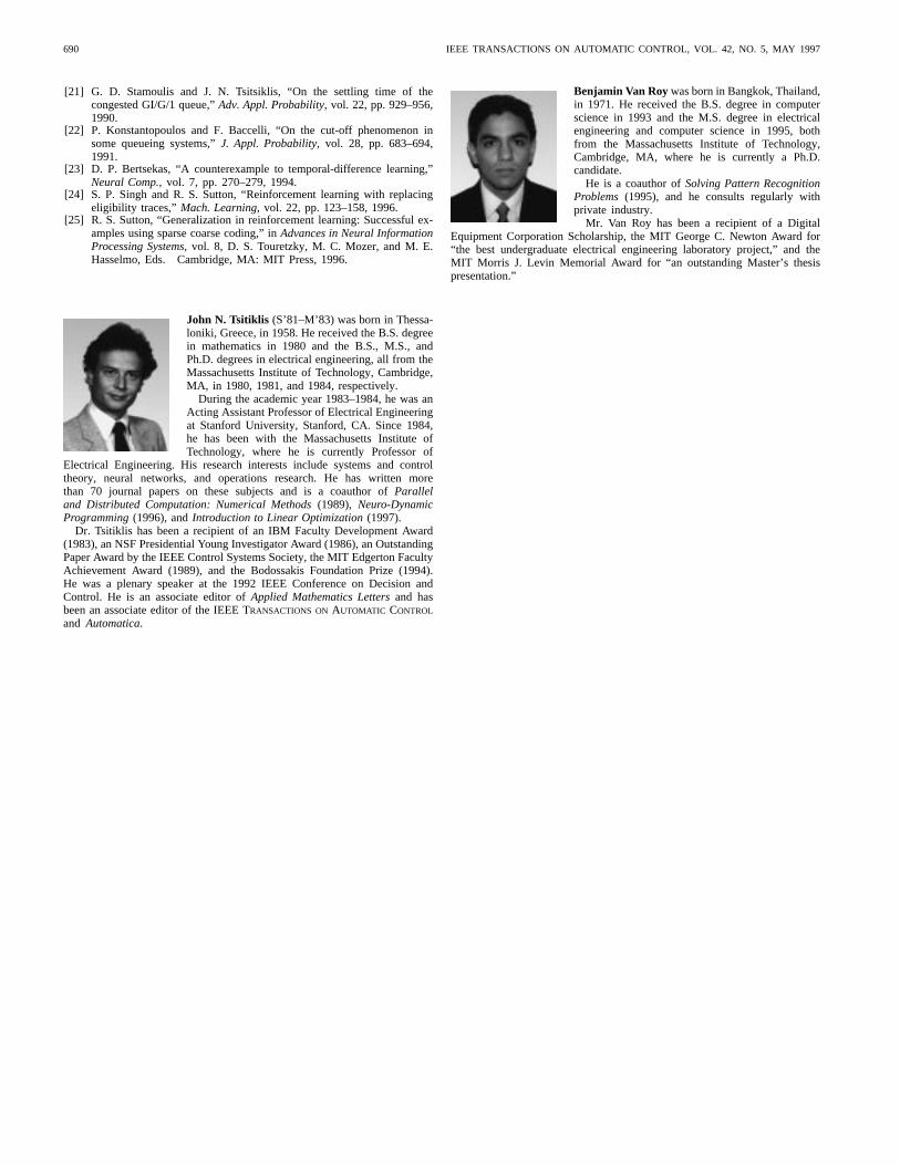
John N. Tsitiklis (S’81–M’83) was born in Thessa-loniki, Greece, in 1958. He received the B.S. degreein mathematics in 1980 and the B.S., M.S., andPh.D. degrees in electrical engineering, all from theMassachusetts Institute of Technology, Cambridge,MA, in 1980, 1981, and 1984, respectively.

During the academic year 1983–1984, he was anActing Assistant Professor of Electrical Engineeringat Stanford University, Stanford, CA. Since 1984,he has been with the Massachusetts Institute ofTechnology, where he is currently Professor of

Electrical Engineering. His research interests include systems and controltheory, neural networks, and operations research. He has written morethan 70 journal papers on these subjects and is a coauthor ofParalleland Distributed Computation: Numerical Methods(1989), Neuro-DynamicProgramming(1996), andIntroduction to Linear Optimization(1997).

Dr. Tsitiklis has been a recipient of an IBM Faculty Development Award(1983), an NSF Presidential Young Investigator Award (1986), an OutstandingPaper Award by the IEEE Control Systems Society, the MIT Edgerton FacultyAchievement Award (1989), and the Bodossakis Foundation Prize (1994).He was a plenary speaker at the 1992 IEEE Conference on Decision andControl. He is an associate editor ofApplied Mathematics Lettersand hasbeen an associate editor of the IEEE TRANSACTIONS ON AUTOMATIC CONTROL

and Automatica.

Benjamin Van Roy was born in Bangkok, Thailand,in 1971. He received the B.S. degree in computerscience in 1993 and the M.S. degree in electricalengineering and computer science in 1995, bothfrom the Massachusetts Institute of Technology,Cambridge, MA, where he is currently a Ph.D.candidate.

He is a coauthor ofSolving Pattern RecognitionProblems (1995), and he consults regularly withprivate industry.

Mr. Van Roy has been a recipient of a DigitalEquipment Corporation Scholarship, the MIT George C. Newton Award for“the best undergraduate electrical engineering laboratory project,” and theMIT Morris J. Levin Memorial Award for “an outstanding Master’s thesispresentation.”

An Analysis Of Temporal-difference Learning With …jnt/Papers/J063-97-bvr-td.pdf · Abstract— We...

Documents

Transcript of An Analysis Of Temporal-difference Learning With …jnt/Papers/J063-97-bvr-td.pdf · Abstract— We...