An analysis of deviations in market bubble moments2 An analysis of deviations in market bubble...

1

Cahier de recherche 2018-02

An analysis of deviations in market bubble moments and their heteroscedasticity

Olivier Mesly

Dr. Olivier Mesly, the contact author, is a university professor of marketing and project feasibility. He can be reached at [email protected].

François-Éric Racicot

Dr. François-Éric Racicot is Professor at the University of Ottawa, Telfer School of Management, 55, Laurier Street East, Ottawa ON K1N 6N5, Canada. Tel.: 613-562-5800 ext. 4757. [email protected]. He is also Associate researcher at IPAG Business School,

Paris, France and at the Corporate Reporting Chair, ESG UQAM.

This article has been accepted for publication by Applied Economics (2018).

2

An analysis of deviations in market bubble moments

and their heteroscedasticity

Résumé: Nous émettons l’hypothèse que les bulles financières de marché sont le possible

résultat de l'interaction entre les produits bénéfiques au consommateur, nommés les Biens («

Goods »), et les produits toxiques (« Bads ») qui se développent à travers trois moments qui se

succèdent de manière systémique : l’attroupement (« herding »), l'essaimage (« swarming » ) et

la calvacade (« stampeding ») , avec des déviations caractérisées par de l’hétéroscédasticité.

Nous utilisons notre modèle stylisé de prédation financière, (« Consolidated Model of Financial

Predation, CMFP), et les données que nous avons accumulées au cours de huit ans de recherche

sur le terrain et l’étude de 30 ans d'histoire du marché américain afin d’explorer les fondements

des crises financières de marché. Nous constatons que la confiance aveugle (ou le biais de

positivité) et la peur de passer à côté d'une opportunité d’entrer ou sortir d’un marché ont un

impact sur les décisions des investisseurs d’investir ou de se rétracter. Nous montrons comment

les marchés sont orientés vers une dynamique de prédateur qui crée des gagnants et des

perdants, en partie à cause de la faiblesse des réglementations les régissant. De plus, nous

identifions une constante k qui imprègne les comportements des marchés.

Abstract: We conjecture that market bubbles may be the results of the interplay of Goods

and Bads (toxic products) which develop through three interlocking moments – herding,

swarming, and stampeding, with deviations marked by heteroscedasticity. We use our stylized

model of financial predation, the Consolidated Model of Financial Predation (CMFP), and data

we have accumulated through in-the-field eight-year research and the study of 30 years of U.S.

market history in order to explore the foundations of market crises. We find that blind trust (or

the positivity bias) and of the fear to miss out on an opportunity to enter/exit a market impacts

the investors’ decisions to invest or retract. We show how markets are driven towards a make-

or-break predatory dynamic that creates winners and losers due in part to weak regulations and

identify a constant k that permeates market behaviors.

Keywords: Bads, Goods, financial predation, consolidated model of financial predation

(CMFP), crisis, regulation, “badfare”

Mots clés : Produits toxiques, produits financiers, modèle consolidé de prédation

financière (CMFP), crises financières, réglementations

3

1. INTRODUCTION

There have been countless market crises in the last centuries, including the Tulipomania

in 17th

century Holland, the Mississipi Bubble in France in the 18th

century, the S&L fiasco in

the USA in the 1980’s and the 2000’s “.com” experience (Rosier, 1987; Kindleberger, 2004;

Rajan, 2010). The 2007-2009 U.S. subprime crisis provides an exemplary model of things

going awry. It impacted consumers, communities, businesses and governments with dire

effects (Brown, 2010). Most of those crises point to the failure of governments to control the

increased toxicity of their markets (Samoa and Shoaf, 2005).

While many authors have offered their views on the causes of market crashes, few have

ventured into modeling them in a systematic way.

Explanations typically encompass such ideas as:

i.The market agents’ behaviors and/or ethics: “the failure of either to behave diligently

or in good faith at any point in the exchange” (Ericson and Doyle, 2003, p. 11); the

tendency to indebtedness Minsky (1975); the window dressing (Neal and Wheatley,

1998); the creative accounting (non-book entry of CDO’s) (Akerlof and Shiller,

2009).

ii.The market agents’s profile: the peer pressure (Scherbina, 2013); various factors

(Aguilera and Vadera, 2008); Machiavellian personalities (Christie and Geis, 1970)

– cold, calculative, sneaky, and selfish).

iii. The presence of structural problems: the asymmetry in portfolio managers’

incentives (Allen and Gate (1999); the ease and speed of transactions (e.g., Internet)

and the ease of access to money (Ferguson (2012); the inability of arbitrageurs to

time the market (Abreu and Brunnermeier, 2003); the income inequality (Iacoviello,

2008; Roy and Kemme, 2012); the network effect (Olsen, 2012); the use of

complexity, often to hide the real risks (Akerlof and Shiller, 2009; Corneil and

McNamara, 2010); the changes in market conditions (employment, interest rates,

4

etc.) (Reinhart and Rogoff, 2008, 2009); the banks’poor management (Jizi et al.,

2014); the inadequate firms’ risk ratings, especially by the Big Three – Fitch,

Moody’s, and Standard and Poor’s (Tremoulinas, 2009; Hellwig, 2009; Gayraud,

2011); the management exuberant bonuses (Graafland and van de Ven, 2011); a

financial culture of Corporate psychopathology (Boddy, 2011); protected financial

networks and their schemes along with poor risk management (Rajan, 2010).

iv.The government: the absence of protection or legal recourse for victims, the lack of

due diligence, the lack of enforcement and punishing power, and the trend towards

deregulation (Ferguson, 2012); the Federal Reserve Bank’s inability to control the

money supply (Friedman and Schwartz, 1963); the government’s laissez-faire

(Gayraud, 2011); the slow speed of the government response (Taylor, 2009); the

unjustified tax breaks (Stiglitz, 2003); unruly deregulation (Krugman, 2009).

In regards the subprime crisis in the US1, the International Monetary Fund (IMF, 2009,

Chap. 2, p. 92) has offered an explanation for it, which emphasizes the existence of spreads

(stretches) and traps (more particularly, the need to refinance once the grace period of the teaser

rates has expired):

“The rising home prices masked the plummeting lending standards, since the

overstretched borrowers found it easy to refinance or sell the house at a

profit. As the impact of rising interest rates kicked in and house prices

flattened, stretched borrowers were left with no choice but to default as

prepayment and refinancing options were not feasible with little or no

housing equity. As defaults mounted, the feedback loop that had amplified

home price growth dragged prices down, which in turn made it impossible

for many overstretched borrowers to refinance to avoid default.”

Inasmuch as the above explanatory efforts have validity, they do not form a complete,

well-rounded capable of explaining or predict market bubbles. To do this, a better

understanding of Goods that are good for the market and of Bads (products with a certain level

of toxicity) is mandatory.

1 See also Bekaert and Hodrick for a discussion on the US subprime crisis (2012, pp. 7-9).

5

In this paper, we first discuss the selling of Bads, and link it to financial predatory

behaviors and our stylized model of financial predation – the Consolidated Model of Financial

predation (CMFP) –, including its psychological version and its notion of predatory net and

traps. We briefly review the four market agents that are active in a bubbling market: consumers

(investors), suppliers (investors in their own right), regulators (such as the SEC in the US) and

predators (who, inevitably, exist in combination with prey). We then delve into details into the

three moments of market crises, supporting our analysis with in-the-field research and US

market data ranging from 1971 to 2013. We show that these three moments present various

levels of heteroscedascity of their standard deviations and that the distribution of the population

during these moments responds to the constant k, a constant that pertains to the CMFP. We

examine the Action and resting potentials of market crises and show how different payoff

strategies explain a market’s three critical crisis moments.

Finally, we conclude by showing that the marketing and selling of Bads generates a

“badfare” economy that the market agents must control and annihilate.

2. THE SELLING OF “BADS”

The 1977 US Community Reinvestment Act (CRA) allowed banks to grant credits to

clients that would have hardly qualified for loans and mortgages. In the years leading to the

2007-2009 subprime crisis, this philosophical stand continued to grow with the mid 1990’s

Glass-Stegall Act revision. In essence, the low income and illiterate citizens as well as other

less favored individuals such as the disabled and older people were considered prime

candidates for a free economy that encouraged spending and home ownership (Tremoulinas,

2009; Gayraud, 2011).

Over the years, the house mortgage industry grew to billions of US dollars, with the

2000-2008 period being infested with predatory mortgages. These predatory mortgages used

teaser tactics such as adjustable-rate loans and teaser rates (as low as 1% over one or two

6

years) in order to attract would-be homeowners (Frame et al., 2008 p. 2-3). The subprime

industry eventually explained 53% of all foreclosures during the critical period.

2.1 Financial predatory behaviors

The term “predatory mortgages” is well chosen. Predatory behaviors during the 2007-

2009 crisis existed with both consumers (those house buyers who hid critical information that

would have disqualified them) and sellers (Cowen, 2008).

Historically, the term “predation” has not been a mere figure of speech (see Tokic, 2014).

Indeed, people readily adopt a predator or prey position (Carney et al., 2010). It has been used

in association with predatory marketing (e.g., the 1890’s Sherman Antitrust Act, the Act to

Prevent Predatory Marketing Practices against Minors2; the 1993 Court case of Brooke Group

Ltd. Vs. Williamson Tobacco Corp.3; the 2009 Mortgage Reform and Anti-Predatory Lending

Act; see also Ordover and Willig, 1981, p. 9) by which prices are set below costs in order to

drive out competition.

The US SEC recognizes predation and discusses it in its Rule 10b-5 of the 1934

Securities Exchange Act: it is an act that “… must be a misstatement or omission that is

sufficiently material to affect an investor’s opinion, that is made intentionally; that the investor

relied upon in making his decision, and that directly caused actual losses” (Ferguson, 2012, p.

191).

In the context of our analysis, we refer to financial predation as more than simply

predatory marketing; this is what we discuss in the balance of this paper.

2 http://www.mainelegislature.org/legis/bills/bills_124th/chappdfs/PUBLIC230.pdf. Accessed May 13, 2017.

3 https://supreme.justia.com/cases/federal/us/509/209/case.html. Accessed June 3, 2017.

http://www.mainelegislature.org/legis/bills/bills_124th/chappdfs/PUBLIC230.pdf.%20Accessed%20May%2013

https://supreme.justia.com/cases/federal/us/509/209/case.html.%20Accessed%20June%203

7

2.2 The market agents at work in a “badfare” economy

The CMFP identifies four market agents: consumers, sellers (producers), regulators and

financial predators. We postulate that these market agents are always present in any and all

markets, at any point in time, to various degrees.

A number of authors have long recognized the vulnerabilities of market agents,

especially that of consumers and at times of sellers as well. These form important

considerations in a predatory market, where market predators capitalize on their prey’s

vulnerabilities. Expressions of vulnerabilities have been listed in part as follows:

i.Cognitive: cognitive biases (Kahneman and Tversky, 1979; Lam, Liu and Wong,

2010); ownership and materialistic values (Shiller, 2005); preys’ financial illiteracy

(Wang, 2009); turnaround expectations (Gjerstad and Smith, 2009); excessive

optimism (positivity bias or blind trust) (Shiller, 2005; Campello and Graham,

2013) and overconfidence (Scheinkman and Xiong, 2003); misconceptions versus

trends (Soros, 2008); money illusion (e..g., the confusion between real and nominal

interest rates) (Brunnermeier and Julliard, 2008); noise trading (De Long et al.,

1990);

ii.Emotional: Fear of losing out on an opportunity (see Lux, 1995); overreaction (De

Bondt and Thaler, 1985); psychological impairment (Danis and Pennington-Cross,

2008, Kamihigashi, 2008); selfishness (Petrick, 2011; Babiak and Hare, 2006);

iii. Behavioral: Contagion (herding) and contagion by refusing to search for proper

information (Shiller, 2005; Calvo and Mendoza, 2000).

In all, there is an extensive literature on the subject of possible causes to market failures

but no model has been proposed so far that takes into account the moments that appear inherent

to them.

8

2.3 The Consolidated Model of Financial Predation (CMFP)

The CMFP is interested in Bads, that is in toxic products that plague a market and that

predators use to lure their prey. Our past research has shown that

kFree riding

QB (1)

where QB is the Quantity of Bads, and k is a constant valued at 1.32, which is active

within the confines of a closed dynamic system (bounded rationality4) which boundaries range

0 to 2.3 (see Figure 3 below). Only a portion of the rectangular hyperbola has a meaning as a

rendition of economic behaviors; outside these boundaries, chaos is considered to prevail. This

curve represents our stylized indifference curve, or put differently, the utility level of the

predatory behaviors: in this case, a consumer is assumed to be free-riding. He takes advantage,

for his own benefit, of the common good regardless of the potential harm he may cause, such

as increasing the cost of the common good. At every point along the so-called Consumers’

predatory indifference curve, the same level of utility is reached. The consumers are indifferent

between benefiting less from free-riding, but obtaining more Bads, or else enjoying the

common good more but having fewer Bads. In both cases, they feel they have achieved an

equal amount of predatory utility.

Figure 1 represents what is going on in the abusive consumer’s mind.

= = =

INSERT Figure 1 ABOUT HERE

= = =

This story only tells half of what is happening. The suppliers, too, are engaged in

financial predatory behaviors in a “badfare” economy. Regulations are represented on the y

4 If bounded rationality is to exist, there must necessarily be some boundaries. Our model is drafted after this

conclusion.

9

axis (in lieu of the costs of the Bads, because regulations represent an inevitable operating

cost).

We have (Table 1):

= = =

INSERT Table 1 ABOUT HERE

= = =

The Suppliers’ predatory indifference curve is a portion of a rectangular hyperbola as

well. At any point along this curve, the utility of the sellers’ predatory actions remains

identical. The sellers may obey to more regulations while refraining from selling more Bads,

or, should regulations be relaxed as was the case in the years prior to the US 2007-2009 crisis,

they may offer more Bads. In the end, sellers enjoy the same predatory advantage (or profits).

Our stylized Edgeworth box illustrates one instance of the dynamic interactions

between consumers and sellers in a “badfare” economy, as follows (Figure 2)5:

= = =


= = =

An equilibrium, albeit fragile, is achieved: the Consumers’ predatory indifference curve

will move away from its point of origin towards the Suppliers’ predatory indifference curve,

signifying that more utility is gained by being deceitful. In the case of the subprime crisis, this

translates into more Bads (more toxic Collaterilized Debt Obligations) being bought for the

5 Note that our framework is represented in a static fashion, unlike the phase diagram used in the Hamiltonian

framework. For an introduction to the latter, see Lambert, 1985, pp. 172-197. For a standard macroeconomic

analyses of steady states and dynamics using phase diagrams, see e.g, Blanchard and Fischer, 1989, p. 46.

10

same amount of free-riding. In the process, consumers believe more and more in their capacity

to beat the market; blind trust builds up6, thus falling into the indebtedness trap of the

predatory suppliers (sellers) – see Figure7 3.

= = =

INSERT Figure 3ABOUT HERE

= = =

The Edgeworth box illustrates a finite environment (bounded rationality) with a zero-

sum game. Its only possible upper limits for the x and y axes is 2.3 if the (Utility) Predatory

curve has a function of

( )k

f xx

(2)

And where k = 1.32 (for reasons seen further along in this text), or

11k

(3)

At k = 1.32, x = 1.15, y = 1.15, one is at the middle point of the Edgeworth box. At x =

y = 1.15 with k = 1.32, the Consumers’ and Suppliers’ predatory indifference curves meet.

Therefore, its extreme upper limit is necessarily of 1.15 2 2.3 .

The boundary of 2.3 expresses the fact that market agents always behave within limits:

their behaviors make sense if there are limits to them, just like there are limits on the amount of

food one can eat at once. Hence, from the market agent point of view, bounded rationality is

expressed by the boundaries of zero (0) to 2.3 when submitted to the constant k8. Market agents

will behave and invest in the market with the limits of their reason, and that limit is an

expression of the k constant, which essentially says that market agents want to remain equal to

6 This is often referred to as a positivity bias.

7 In this system, the operating area (where the decisions to invest occur) is considered to be constrained by 2.3•

2π/4 or equivalently (1 + k) (π/2) or equivalently: (1 + k) / 2(k – 1). 8 Our past research has shown that this is the case for economic behaviors.

11

themselves (hence, its, relationship to π). At k =1.32, there is equilibrium, but any k larger than

1.3 tends towards unfairness, possibilities of retaliation and chaos. The maximum value that k

can reach is 4.6 (at which point, x = 2 and y = 2.3, the uppermost limit), hence nearing the

Feigenbaum value of 4.669, which expresses chaos. It can be justifiably assumed that the entire

system, in the market agent’s mind, is closed, dynamic, and governed by bounded rationality9.

The Suppliers’ predatory indifference curve also moves away from its own point of

origin sitting on the upper right corner of the stylized Edgeworth box, signifying that the sellers

are better at cheating the regulations: they can thus sell more Bads and feel they can beat the

market10

. Consumers and suppliers become increasingly deceitful, and thus, in actual fact, the

market becomes riskier (see Bolton and Scharfstein, 1990).

A “badfare” economy sees in an increase in toxicity, in Bads being available on the

market. At that Predatory Point of Equilibrium, we posit that there is no economic profit,

which discourages potential competition. The sellers that are already active in the market

become increasingly deceitfully in order to gain a larger share of it. In the process, those less

savvy or conspicuous are evicted from the market, allowing for more concentrated abuse. The

cases of AIG or Lehman Brothers speak volume to that effect, all the while Goldman Sachs

ended up stronger than ever. Consumers smart or capable enough to avoid the sellers’

indebtedness trap (a “poverty trap” as put by Mehlum, Moene, and Torvik, 2003) fight each

other for the Bads that are becoming available. Instead of betting on future Goods, the market

agents end up gambling more and more on future Bads (QBadst + 1).

9 In the CMFP (e.g., Mesly, 2013a, 2013b, 2014a, b, 2015a, b, Mesly and Bouchard, 2016; Mesly and Racicot,

2017) studies has shown that the budget line of the consumers is expressed by B(x) = 2.2-0.9x. The same logic

applies to the seller. This means that their budget lines cannot actually parallel each other in an Edgeworth box: a

perfect, stable equilibrium is impossible. Only a dynamic equilibrium can prevail and the information each

receives is necessarily asymmetric. Furthermore, the consumers’ satisfaction (expressed by S(x) = x + 2k/x – 2k1/2

)

is suboptimal at the perfect point of equilibrium and this is true for the sellers as well; hence, each has an incentive

to depart from and move further away from the point of equilibrium. In short, consumers and suppliers realize

they can fare better by being a little bit more deceitful (Mesly, 2014a). 10

Bernard Madoff is an exemplary case (e.g., see Gregoriou and Lhabitant, 2009).

12

The sellers are driven by the fear of losing out on the opportunity to benefit from weak

regulations for their selfish interests and tend to rationalize their excesses (Milgrom and

Roberts, 1982), ever so eager to increase their exuberant wealth. More profits can be obtained

by disregarding other market agents’ welfare. Sellers need to bet on the ups or downs of the

market (a trap) to deceive consumers and competition and consumers need to engage further

into debt (a trap) in order to improve their market position, i.e., their possession of Bads. It is

to the best advantage of all deceitful market agents to deceive the others: Bads products lead to

bad behaviors, and vice-versa.

This stampede phenomenon is represented in Figure 4.

= = =


= = =

Along the way, economic losses are incurred. Consumers and suppliers’s options

diminish and their traps force them to spend more and more to get out of their pits. As toxicity

reaches its upper limits, bankruptcies and foreclosure sprawl; the crisis is in full effect.

2.4 The predatory net and the traps

Predatory traps – whether in the form of indebtedness or one-sided market gambling –

are one out of ten components of what is referred in our CMFP as the predatory net (See

Mesly, 2014a) and competitive advantage in a closed, dynamic duopolistic system –

consequences for regulatory authorities). This net is composed of five structural components

(sine qua non conditions of the existence of the net): predators, prey, tools (predatory

mortgages, Special Purpose Entities), harm (the losses that the market agents incur11

– see

11

According to the U.S. Government Accountability Office (https://www.gao.gov/. Government Accountability

Office, 2004, p. 3. Accessed June 13, 2017), predatory mortgages are transactions that “contain terms and

conditions that ultimately harm borrowers.”

13

Ordover and Saloner, 1989; Cabral and Riordan, 1997) and a surprise effect (achieved by being

deceitful). The net is also expressed by a strategy that includes identifying the prey’s

vulnerabilities (e.g., an illiterate house buyer absorbed by the housing market herd), setting up

bait (teaser rates), forcing a decision (by pressuring the eager house buyer), setting up a trap

and finally subduing (by forcing foreclosure or bankruptcy).

The net is illustrated as follows (Figure 5).

= = =


= = =

Predators are motivated by selfish gains (Tulogdi et al., 2010). Additionally, they are

cold (displaying little if not no regard for their prey – see Ferguson, 2012), calculative (Meloy,

1997), and sneaky (Graham, 1996). To that effect, Shiller (2005, p. 76) notes: “When clever

persons become professionals as deceiving people, and devote years to perfect their act, they

can put seemingly impossible feats before our eyes and fool us, at least for a while.” Prey are

naive and defined by their vulnerability12

; they are reactive rather than pro-active13

.

In regards the US subprime crisis, the predatory web translates as follows (Table 2):

= = =


= = =

12

A disproportionate number of victims of market fraud are 65 years old or more (Tongren, 1988; Yoon et al.,

2005); these people see a decline in their cognitive capabilities with age (Charles and Piazza, 2009; Moschis,

Mosteller, and Fatt, 2011). 13

In natural ecosystems, predator and prey populations maintain an equilibrium and this guarantees the survival of

both (Bonsall and Hassell, 2007).

14

2.5 The psychological framework of the investor, according to the CMFP

The above-described market phenomenon does not happen in a psychological vacuum.

Quite the contrary. It is based on the psychology of consumers and sellers that the market

behaves the way it does, engages in bubbles and suffers crashes. Hence, our CMFP, based on

many years of field research and secondary data collection, has provided the following model,

which has found some neurobiological correlates (Hostinar, Sullivan, and Gunnar, 2014; Rolls,

2006; Lang, Davis and Öhman, 2000; Akirav, 2013; Gregg and Siegel, 2001; Gregg and Siegel

(2003), including in fMRI studies14

(Figure 6):

= = =


= = =

This is a classical model that summarizes many studies based on perceived risk, which

the CMFP estimates to be the ratio between the sense of control the investor has over his

investment and the transparency he receives from the object of his investment. Risk assessment

provides self-protection (Frijda, 1986; Lazarus, 1991; Levenson, 1994; Ekman, 1999; Keltner

and Gross, 1999; Kunzmann, Kappes and Wrosch, 2014) that may ensure survival in the

marketplace.

14

Most notably, the hypothalamus is the center of predatory (lateral) and prey (medial) behaviors. It controls all

major homeostasis-related activities which ensure the survival and equilibrium of the body; it has a one way

(instead of a bidirectional) link to the pituitary gland, which forces hormones produced by both to travel through

the entire body before returning to the hypothalamus with bodily information (Squire et al., 2003; McCullough et

al., 2007; Berthoud and Münzberg, 2011, Hinds et al., 2010). This is in line with the CMFP which has an

unidirectional link between perceived risk and trust. Furthermore, the fear “network” includes the amygdala (Aue

et al., 2013; Dilger et al., 2003; Amaral, 2002, Schaefer et al., 2014) of course,, but also the the orbitofrontal

cortex involved in decision making (Cardinal et al., 2002; Dolan, 2002), the anterior cingulate cortex (responsible

for error detection – Paulus et al., 2004), the periaquiductal gray (PAG) (Gray and McNaughton, 2000, p. 31),

and the insula. The Ventral tegmental area (VTA) is the center of reward. In other words, the CMFP has some

neurobiological correlates.

15

The buyer wants to feel he is in relative control while expecting to be fully informed

about his investments, such as buying multiple houses. Similarly, the seller who invests his

time and effort in dealing with a customer expects to be able to secure his repayment schedule

and to have enough information on him to feel that he is relatively reliable (Figure 7). The

higher the perceived risk, the lower the trust, trust being a core construct in economic theory

(Stiglitz, 2003; Akerlof and Shiller, 2009). The more the trust and, concurrently, the impression

that both market agents can win by dealing with each other, the easier the decision to invest.

The better the returns on the investment resulting from the decision to invest, the lesser the

perceived risk. In a situation of blind trust (extreme positivity bias) (Smythies, 2009; Dezsö and

Loewenstein 2012)15

, the perception of real risk is lessened (Odean,1998), and the cycle tends

to spin out of control (Mesly and Bouchard, 2016)16

. As explained by Lux (1995, p. 883):

“Hence, speculators are not simply blind followers of the crowd: they quickly react to others’

behavior in order not to miss profit opportunities (…)”. The market agents’ behaviors, then,

tend to worsen with time: they become increasingly emotional (Shefrin and Statman, 1985),

biased or irrational (Kahneman and Tversky, 1979), delinquent (Danis and Pennington-Cross,

2008), inconsistent (Smith, Suchanek, and Williams, 1988), or even pathological (Kamihigashi,

2008).

As for fairness (Figure 6), it has been the subject of many legal battles – see, for

example, Fremont Invest & Loan vs. Commonwealth of Massachusetts during the subprime

crisis. In particular, people who feel they have been treated unfairly seek compensation

(Bäckman and Dixon, 1992) – people who had been deprived of the opportunity to buy a home

went for it with a vengeance when the solvency criteria were relaxed by the US government’s

policies.

15

Blind trust can affect all market agents (Loughran and McDonald, 2011). 16

“People trust others even when there is no guarantee that the trustee will respond benevolently.” (Fetchenhauer

and Dunning, 2009, p. 264)

16

3. THE THREE MOMENTS OF A CRISIS

Our stylized model conjectures that there are three key moments in any financial crisis,

which we refer to as the herding, swarming and stampeding moments. Swarming includes

herding; however, the reverse is not true. Similarly, stampeding includes swarming, but the

reverse is not true. Herding (Dass, Massa, and Patgiri, 2008; Olsen, 2012; Biacabe, 2000)

occurs when a large number of a given population of market agents regroup towards a common

goal, building wealth, out of the fear of missing out on a market opportunity. Preys act

spontaneously (see Gregg and Siegel, 2001) and tend to “Keeping up with the Joneses” (Dupor

and Liu, 2003). As such, they are easily influenced.

Each market agent believes each one will win. Strategically, there is just one alternative

and no option (as an option implies at least two alternatives): invest.

We have:

Investor Sellers (e.g., sells a predatory mortgage) Win

Investor Buyers (e.g., buys a house with a predatory mortgage) Win

Swarming occurs when this herd, and newcomers that eventually join from current

herds in the making, join and focus on maximizing their gains, out of fear of missing out on the

same opportunity, but with a defined target – specific market or financial targets are the subject

of such market moment. At this point, the market agents consider that some may win and some

may lose, but the gain of one may not cause the loss of the other. Furthermore, there is one

option and thus two alternatives: invest or wait.

Going back to Figure 6 and the psychological model of the market agents, it can be

seen that both agents (seller and buyer) judge that the risk is minimal (hence the fear of missing

out on a great opportunity increases), and as the risk is deemed minimal, they each nurture trust

towards each other. With a sense of fairness added to this dynamic, they tend to cooperate: the

17

seller sells the predatory mortgage to the buyer and the buyer buys the predatory mortgage

from the seller. Both envision making money and as this actually materialize, the perceived

risk diminishes further – the positivity bias inflates, blind trust gains ground. Our stylized

payoff matrix is in fact the game matrix of payoffs and is a representation of the “strategic

form”17

.

Two players Added alternatives if there are more than

two market agents

Sellers Sell Wait Sell Wait

Buyers Buy Wait Wait Buy

Here, if there are only two market agents (consisting of a seller and a buyer), if the

seller sells, the buyer feels compelled to buy given his fear of missing out on the opportunity.

If the seller wait, the buyer must wait. But there are other sellers or buyers, their alternatives

may be enhanced: the seller may sell and the particular buyer ay opt to wait, so that the seller

will seek another buyer. The seller may wait, but the buyer may chase another seller. This is a

fragile equilibrium where the seller and the buyer may feel they have achieved their best

strategy; changing it would make them worse off. However, trying to improve it may be to the

detriment of the other, which could lead to retaliation (e.g., the seller giving the market

opportunity to another buyer or refusing to lend a predatory mortgage). The gains and losses

are not predetermined. Given that swarming is a moment that follows herding, it is fair to

assume that there are always other sellers and buyers. In fact, as more of those market agents

join in, the higher the pressure (the fear of missing out on the opportunity) to sell and buy. All

looks good, nothing looks bad.

Some market agents may feel they have not been treated fairly: after all, the

justification given for creating the predatory mortgages was precisely that the Bush

government wanted to give those who had not qualified in the past a chance to own a home.

For some investors (the sellers investing in the buyers and selling them more predatory

17

The extensive form is a more in-depth representation of a game. For a detailed discussion on this, see Varian

(1993, chap. 15).

18

mortgages and the buyers borrowing more money to buy more houses), the positivity bias

inflates and blind trust turns out to be quite convenient. Not everything looks good.

The last but not least moment is stampeding. It necessarily follows swarming. Here,

market agents act out of fear to miss the opportunity to enter or exit the market. There are thus

three alternatives in this zero-sum game: continue investing, wait, or exit. The gain of one is a

loss for the other and everyone rushes to maximize gains, hence the stampede.

Here, the following scenarios are possible; there is no in-between and it is a make-or-

break situation. This is truly a zero-sum game in a finite environment (for example, there are

simply, only so many houses for sale in the market) and this finite environment makes

retaliation possible (otherwise, market agents could escape the toxic environemnt and move

somewhere else where they would be immune):

Sellers Win Loose

Buyers Loose Win

Obviously, the losers will exit the market, narrowing down the options to find other

market agents for those remaining; all the while, those who stay and win see their negotiating

power and market share (of Bads) increase. This continues until an apex of toxicity (Bads

overwhelming the Goods) is reached, past which a sharp decline ensues.

Going back to Figure 6 again, it can be seen that both agents (seller and buyer) judge

that the risks are high. Those who operate with a maximal degree of positivity bias (blind

trust) cannot see that the market is filled with Bads. They keep investing. But the Goods of

ones and actually the Bads of the others; the blind investors do not realize their Goods are

actually Bads, that their pools of mortgages, for example, are infested with toxic unsustainable

mortgages. For the predators, the Bads are Goods: they make money off them as long as they

can find naïve buyers they can lure.

19

As can be intuitively sensed, there is an accumulation of uncertainty (perceived risks),

expressed by an increased level of heteroscedasticity of the moments’ deviations.

3.1 First moment: Herding (σ2

h)

The average k for the 1,835 respondents that we investigated in a seven-year research

on predatory behavior equals 1.35, with the constant k being expressed as per equation (3) seen

above.

Our analysis of the sample distribution, which is assumed to have been in a herding

moment, suggests a distribution as follows (Table 3):

= = =


= = =

The vast majority of the sample population is concentrated around the mean, but the

level achieved by the ratio predator/prey stretches rapidly and considerably near the mean.

Based on this data (see Table 4), the estimated distribution for the first moment with variance

of 2h (with h referring to the herding moment) is therefore related to the distribution function

of

20.5 /0.32

( ) 1.32 2.71 hx

hf x

or

21 0

2 1( )1

hx

kh

kf x e

(4)

where μ = 0.

This versus a Gauss’ normal distribution curve expressed by:

20

2

2

1

21( )

2

x

f x e

(5)

Table 4 :

In a herding situation, the game between the seller and the buyer is played as follows:

Sellers sell Goods Sellers sell Bads

Buyers buy Goods 2.30, 2.3018

1.73, 0

Buyers buy Bads 0, 1.73 0, 0

Note: Pairs of payoffs in the diagonal represent our stylized version of Nash equilibria with top left quadrant being the preferred one.

The payoffs for the seller and the buyer is $ 2.30 each if they both stick to Goods

(excitedly so). There are no incentives to buy Bads, so that if the seller tries to sell Bads, he

ends up with nothing because the buyer (or consumer) will continue to buy Goods.

3.1 Second moment: Swarming (σ2

s)

Our estimated distribution for the swarming moment with variance of σ2

s (with s

referring to the swarming effect) has a hypothesized function of

2

0.5 / 0.68( ) 0.66 2.71 s

xsf x

or

21

2 2( )2

sx

ks

kf x e

(6)

This second moment (swarming) is thus somehow influenced by the first moment

(herding) because the value 2 reflects the fact that it is the stage after stage 1, that of herding

(see Table 5).

= = =


= = =

18

We could consider this pair of payoffs as what could be called our stylized Nash equilibrium.

21

In a swarming situation, the game between the seller and the buyer is played as:


Buyers buy Goods 1.15, 1.15 1.73, 0.58

Buyers buy Bads 0.58, 1.73 1.15, 1.15

Notes: The stylized Nash equilibria appear on the diagonal of the payoff matrix of the swarming moments. The two equilibria are actually

equal, which causes a hesitation between the market agents. The sellers and buyers hesitate between selling more Goods or else more Bads, and equivalently, the buyers hesitate between buying more Goods or more Bads. This renders the interaction volatile, so that both market

agents will be driven towards the third moment (stampeding, which is explained below) in an attempt to reach a single optimal position.

The payoffs for the seller and the buyer is $ 1.15 each if they both stick to Goods or to

Bads. There are incentives to sell or buy Bads because the payoffs are greater than in other

scenarios but this implies a winner and a loser.

3.1 Limit (σ2

limit)

Before we jump to the third variance, that of stampeding, let us examine what happens

at the limit of the system (see Table 6), at x = 2.3. We have a hypothesized a distribution

function of

2

limit0.5 / 0.98

limit( ) 0.57 2.71x

f x

or

2

limit1

2 2.3limit( )

2.3

x

kkf x e

(7)

= = =

INSERT table 6 ABOUT HERE

= = =

Thus, at k = 1.3 and an associated σ of 0. 30 (for a σ2 of 0.90), the sample population

acts it its most normal (rational) manner.

22

In a limit situation, the game between the seller and the buyer is played as follows:


Buyers buy Goods 1.15, 1.15 1.15, 1.15

Buyers buy Bads 1.15, 1.15 1.15, 1.15

Notes: In this particular case, all four options (quadrants) are equal, thus the market agents cannot make a final choice because every other option is equally acceptable. Hence, they constantly move back and forth between the four options, unable to maximize their positions. At the

limit of such system, rationality is maximized, that is, it is bounded (the Edgeworth box is bounded by the maximum value of 2.3 and the

minimal value of zero). Past this state of affairs, there are no other venues but irrationality.

In this scenario, there is a dynamic predatory equilibrium; there is a constant incentive

for both players to try Goods and Bads, at all times. Along those lines, Besanko, Doraszelski

and Kryukov (2014) have suggested that price predation tends to trouble equilibrium, as can be

inferred from the three critical moments exposed here.

3.2 Third moment: Stampeding (σ2p)

Past the limit of 2.3 of the closed dynamic system, however, the stampede moment with

a variance σ2

p is hypothesized to be related to of

2

0.5 / 1.68( ) 0.44 2.71 p

x

pf x

or

2

1

2 3( )

3

px

kp

kf x e

(8)

Graphically, this is represented as follows (Table 7):

= = =


= = =

In a Stampeding situation, the game between the seller and the buyer is played as

follows:


Buyers buy Goods 0.58, 0.58 0, 2.30

23

Buyers buy Bads 2.30, 0 1.73, 1.73

Notes: The optimal position for both market agents is actually the worst market condition, where both market agents have the strongest incentives to buy and sell Bads. Thus, as those market agents move along the moments of the crises as hypothesized in our model, they have

no choice but to move, literally, from good to bad, and from Goods to Bads.

The payoffs for the seller and the buyer is only $ 0.58 each if they both stick to Goods;

Bads is the way to go but there is some hesitation because Bads could turn out to be good ($

2.30 payoff) but then, this would require that one of the other player plays against market rules

by way of selling or buying Bads.

3.3 Summary of the three moments of a market bubble

In summary, the CMFP has identified three unique moments in financial crises.

Herding consists of a relatively spontaneous reaction. As such, it is relatively disorganized. Its

aim is to acquire a Good that is perceived as being essential. Herding is based on fear: fear of a

clear and present danger. For example, consumers will sign for predatory mortgages for fear of

missing out on the opportunity to invest in the market and make quick money by flipping

houses. Swarming is a medium- to long-term organized action. The goal is not to escape –for

example, a poor economic living condition – but to as many Goods as possible, whether they

are essential or not (hence, during the subprime crisis, consumers would acquire multiple

houses that they, obviously, did not need, but that other buyers could potentially have needed).

Herding is a pre-condition to swarming and swarming is a pre-condition to stampeding.

Swarming and is equivalent with greed. Stampeding occurs when market markets destroy each

other in their attempt to gain a stronger position in the market in fear of missing out on the

opportunity to capitalize on it or else to exit it in fear of losing everything. Stampeding is also

an expression of greed that, however, leads to panic (see Thomsett and Kahr, 2007)19

.

The three moments can be captured as follows (Table 8):

19

An example of such dynamic is the Wal-Mart’s 2008 Black Friday. Overexcited consumers lined up over night

(for Goods they thought they needed desperately), swarm the stores when the doors opened early in the morning

and stampeded each other in their fight to access Goods that, in the end, they did not really need. Consumers

turned a blind eye to the fact that Wal-Mart prides on “everyday low price” anyway, and on the fact that their

time and efforts boosted the actual price of acquiring the Goods, so that in the end, these Goods were actually

more expensive than if they were sold at the regular price.

24

= = =


= = =

In a time sequence (with the payoffs being shown underneath the graphs), we obtain

(Table 9):

= = =


= = =

In bold is the payoff table suggesting the likely behavioral scenarios. One can see how

the market moves from Goods to Bads, with the Bads promising more than the initial

equilibrium stage. At the very end of the stampede, a new state of equilibrium arises.

We conjecture that the evolution of a market bubble goes as follows: an economic

system functions at its limit and displays rationality given the circumstances; it behaves

normally. At some point, there is a herding moment by which the investors regroup around a

narrower range of options with high expectations; this acts a spark on the system. The system

tends to stabilize in the swarming moment, when everyone finds somewhat of a winning

position in the market, which explains why the uptrend of a bubble is slower than the actual

crash, which is far more brutal. The investors eventually move away from the fragile, dynamic

predatory equilibrium and enter into the third moment, that of stampeding, by which extreme

decisions and actions are taken, and this by a growing mass of investors. At this point, the

economic system is off limit and crashes.

25

4. THE RISE OF THE HETEROSCEDASTICY OF THE MOMENTS’ DEVIATIONS

We hypothesize, based on our analysis of the predatory dynamic that took place in

2007-2009, that in fact the rise of the heteroscedasticity, which refers to the increasing change

in the variance of the distribution pertaining to the three bubble moments, is actually due to

two inputs, that of “Goods” and that of “Bads”.

What we notice is that there is a spark (moment 1: herding) in the marketing of

financial products (e.g., mortgages) that, at first glance, seem inoffensive. However, as time

goes one, the offer of those “Goods” is replaced by that of “Bads” (increasingly toxic financial

products such as predatory mortgages, Special Purpose Entities and Collateralized Debt

Obligations in which risks are hidden in a pool of mortgages, some highly toxic). The spark of

“Bads” goes somehow unnoticed because it is not as salient as that of the “Goods” that

preceded it. Henceforth, the market becomes increasing volatile; the standard deviation around

the mean of the “Goods” increases as the presence of toxic products, the “Bads” increases, and

the standard deviation around the mean of those “Bads” widens as well as a result of predatory

pressures. In fact, market agents become more and more emotional and less and less rational

(see Lerner and Keltner, 2000).

This can be represented as follows (Table 10):

= = =


= = =

As investors (e.g., house buyers attracted by the low interest rates) herd towards to

Goods (the appealing mortgages), market predators devise and market an increasing number of

Bads, luring the naïve investors in their trap. The point where the Goods curve meets the Bads

curve is called a decision revolving door: at that point, the investor does not know if the Goods

26

are actually bad, and if the Bads are actually good. Thus, he debates, goes round and round,

just like most of the other investors, who each try to catch each other to the game but

obviously, catching someone in a revolving door is a lost case.

The result of the above dynamic is actually a graphical summation of what happens to

the variances in the three moments of the market bubble (Table 11):

= = =


= = =

On the right side of Table 9, we put an equivalent of what happens on the left side but

plotting the y-axis as “type of market” (positive or negative) with the negative market

witnessing the Bads taking over the Goods. We call the initial moment the Action potential and

the return to an equilibrium the Resting potential. From the beginning of the Action potential,

at moment one, that of herding, to the end of the third moment, once the bubble has exploded

(at the end of stampeding moment), predatory behaviors have developed in number and

intensity. The Action potential generally results from a fundamental change in the market – for

example, the elimination of regulations or the creation (as times concomitant) of new

investment opportunities, such as predatory mortgages.

Examples of the Action-Resting potentials are found in the market place. Using the HPI

(Historical measure of Financial Predation Index – see Mesly, 2015b and Appendix 1), a

research has shown the following two instances (1982-1983; 2000- 2001) – see Figure 7:

= = =


27

= = =

As can be observed, the shape of the bubble curves is remarkably similar to what is

predicted by the model (Table 12):

= = =


= = =

Since we assume in the CMFP that the Action-Resting curve shape is the result of a

particular interplay between Goods and Bads as per Figure, we tend to posit that the 1985,

1993, 2000 and 2007-2009 markets were indeed plagued with Bads. This is particularly well

documented for the 2007-2009 crisis, of course. Of interest, the 1993 crisis did not achieve its

full resting potential and rapidly is followed by another crisis, that of the .com bubble.

According to our view, market crashes occur in the mandatory presence of Goods and

Bads, with Bads taking over the Goods over time. Market crashes are thus due to the

overwhelming presence of market predators. In other words, heteroscedasticity is a expressing

of the spread that affects Goods and Bads.

5. DECISION TO INVEST IN A MARKET MARKED BY ITS MOMENTS’ THE

HETEROSCEDASTIC DEVIATIONS

The heteroscedasticity of the standard deviations (or, put differently, of the variances)

with each deviation being dependent on the previous one (with each moment the result of the

previous moment), makes the system volatile and bound to crash. This heteroscedasticity

means that investors make fewer rational decisions, and each wrong decisions drives them

towards more errors (i.e., towards chaos). Indeed, studies have demonstrated that a negative

outlook and a higher number of cognitive errors are correlated whereas a positive outlook has

28

no correlation with cognitive errors (Fetterman and Robinson, 2011). A positivity bias seems

to act as an immune system against errors.

The decision to invest (DI) is a make-or-brake situation, as expressed by the functions20

( )( )aDI E r k (9)

where 1( ) ( )a f a m f tE r r E r r QBads is our own stylized CAPM model

21, and

/

3

t m

t

; ra is the return on asset a; rm is the market return; and rf is the risk-free rate;

with the market return rm being captured in the psychological model of the CMFP (See Figure

9); the decision to invest is conceived as the result of a combination of trust and fairness; ψ is

blind trust or equivalently the positivity bias or the investor’s belief that he can beat the

market; φ is the investor’s fear of missing out on the opportunity (to enter or exit the market);

σt = standard deviation of the moment t (herding (h), swarming (s), or stampeding (p)22

. As for

σm ,this refers to the standard deviation of market returns.

For example, some investors may be sitting on the herding moment while others may

have already reached the stampeding moment. We posit that

1( ) (1 )h s p t t tf QB k QB QB (10)

where ԑ signifies chaos (hence, ԑ is a standard function of chaos), that is, the sum of the three

standard deviations which may all exist at the same time across different layers of the market23

.

Because QBt+1 is not known, as it represents the selling of Quantities of Bads in the

future (t + 1), it really is an expectation. Hence, the chaos factor is, for the investor, the

expectation that future Bads will come or come back and haunt him, (or put differently, that he

20

The (k + Ψφ) indicates the make-or-break situation: when the second part of the equation (Ψ

φ) equals 0 (there is

no variance σt), it is a make. When it equals to 1 (complete blind trust), so that the total (k + Ψφ) equals 2.3, the

limit of the system is attained and it breaks. 21

Our model is analogous to the well-known build-up approach (Pinto et al., 2015, p. 75) 22

As expected, vulnerable people make more mistakes than those in control. For example, older poeple make

more mistakes in estimating rate changes that affect the marketplace (Agarwal et al., 2008). 23

As expected, vulnerable people make more mistakes than those in control. For example, older poeple make

more mistakes in estimating rate changes that affect the marketplace (Agarwal et al., 2008).

29

will be deceived). What one market agent will impact what the other does (Hellwig, 2009). Put

differently, it is the possibility that market agents will retaliate against him given his

involvement with Bads24

. As long as he feels he can cheat the system and outsmart others

(regulators, consumers, other providers), he has no reason to fear, no reason to attribute a value

other than zero (0) to ԑ, and hence has no barrier to continue investing. The fear of retaliation

can also be calculated by the cumulated variances of the three moments at the moment of

measurement since these variances infer that there has been a “distantiating” movement away

from normality.

We can reformulate the Expected return equation for asset a as follows:

1( ) ( )a f a m f tE r r E r r QBads (11)

The investor will want to maximize the first part of the equation (gains) and minimize

the last part (losses), that is QBadst+1. His decision to invest is therefore an attempt to

maximize gains, minimize retaliatory losses (expressed by QBadst+1 while being influenced by

a possible blind trust (positivity bias) given his fears to miss out of the market

opportunities25

so that

( )( )aDI E r k where 1( ) ( )a f a m f tE r r E r r QBads (12)

Chaos (or QBt+1) is the fear of retaliation or equivalently the actual market deviations

showing increasing cumulative heteroscedasticity26

. It requires that the investor is actually

capable of perceiving the Bads; in other words, that he does not suffer from blind trust.

24

As seen when discussing equilibrium, consumers and sellers have an incentive to become more deceitful. But

the DI function indicates that as each one become so, the other retaliates by becoming in turn more deceitful. Each

engage further into the trap of the other. The market, of course, longs for equilibrium amidst various momentums.

Thus, equilibriums and momentums are critical in market dynamics. 25

The formula recognizes the importance of emotions, such as regret, in decision making (Damasio, 1994;

Zeelenberg et al., 1996; MacGregor et al., 2000; Sevdalis, Harvey and Bell, 2009; Seiler, Seiler and Lane, 2012). 26

Neurobiologically, nocive stress induces a reduction in the perfomance of critical functions with leads to the

make of more decision-making errors (more variance). Under nocive stress, the amygdala, the center for emotion

and anxiety located in the brain, increases, while the hippocampus (critical for learning and memory) and the

prefrontal cortex (responsible for decision-making) shrink (Bear et al., 1996; Lupien, et al., 2009). It has been

found that emotions such as fear affect judgement (Angie et al., 2011).

30

We can relate this equation to our stylized CMFP’s psychological model. Let us set

QBt+1 as lack of fairness, since it indicates that the market agent will eventually suffer from the

actions of another market agent, with the possibility of on-going retaliation. It can be said that

the decision to invest (to cooperate) – DI –, is a function of risk assessment (fear), of a

positivity bias (leading to blind trust), augmented by fear such as the fear of missing out on the

opportunity to exit the market27

when the market is, truly, bad.

Hence, we have the rendition of the DI formula in our stylized psychological model of

financial predation as follows (Figure 8):

= = =


= = =

At σt = σh (first moment) or at σs (second moment), this is considered a possible make,

depending on σm. At σt = σp (third moment), this is considered a possible break, depending on

σm; The break occurs when QBt+1 is greater than the first portion of the equation: then, there is

no more win but only losses.

At σt = σlimit, this is considered a dynamic predatory equilibrium, so that σm is assumed

to permit such equilibrium.

6. CONCLUSION

Our analysis shows that a financial market operates under the influence of two forces:

equilibrium (necessarily dynamic) and momentum28

(expressed by the moments), which dictate

the right move to make at the right time. The essence of predatory behavior, thus, revolves

27

This is equivalent to the “option to exit” used in real options analysis. For more, see Mun (2006). 28

Mometum here is referred to the term as used in finance (e.g., Pinto et al., 2015).

31

around the interplay between equilibrium and momentum. The equilibrium is necessarily

unstable because at its point, the Budget curves of the buyers and sellers cannot perfectly

parallel each other and their respective Satisfaction curves are suboptimal. Only by deceiving

can the situation of one market agent appears to be improved, to the detriment of the other

market agent. Hence, Bads are eventually created.

Financial crises are the making of Goods and Bads in an evolving interplay that goes

from Action (momentum) to Resting (equilibrium) potentials. At the heart of this dynamic is

fear, fear to miss on the opportunity to enter or exit the market.

During a market crisis, the heteroscedasticity of the variances changes – it is far from

stable, moments evolve and cumulate. This instability (or ambiguity) generates more fear.

The CMFP considers that the four market agents – buyers, sellers, regulators and

predators – are confined by a mental frame that has its own limits of rationality (a measured

bounded rationality in our model). Our model attempts to set an analytical foundation of such

closed dynamic system and recognizes k as the constant that regulates the market agents’

behaviors, and ultimately, their decision to invest or disinvest (enter or exit the market).

Through research in the field with nearly 2000 participants, data analysis of the US market

over the last 30 years, and our analytical framework, we have found k to be equal to 1.32

within the boundaries of a closed dynamic system of rationality stretched between the limits of

0 and 2.3. It turns out that k = 1 + 1/π.

The decision to invest is a make-or-break one. Greed and panic build up as a

consequence of present and expected market behavior. The market agents compare their

vulnerabilities to the forces (especially to the Bads) of the market to determine which action

course to take29

.

29

As mentioned, we found some neurobiological correlates to the CMFP. This is normal: what appears in the

market is generated by humans, who are controlled by their brains.

32

7. REFERENCES

Abreu, D., and Brunnermeier, M. K. (2003). Bubbles and crashes. Econometrica 71(1), 173-

204.

Agarwal, S., Driscoll, J., Gabaix, X., and Laibson, D. (2008). The age of reason: financial

decisions over the lifecycle. American Law & Economics Association.

Aguilera, R.V., and Vadera, A.K. (2008). The dark side of authority: Antecedents,

mechanisms, and outcomes of organizational corruption. Journal of Business Ethics 77(4),

431-449.

Akerlof, G.A., and Shiller, R.J. (2009). Animal spirits: how human psychology drives the

economy, and why it matters for global capitalism. New Jersey: Princeton University

Press.

Akirav, I. (2013). Cannabinoids and glucocorticoids modulate emotional memory after stress.

Neuroscience and Biobehavioral Reviews 37, 2554-2563.Allen, F., and Gale, D. (1999).

Bubbles, crises, and policy. Oxford Review of Economic Policy 15(3), 9-18.

Allen, F., and Gale, D. (1999). Bubbles, crises, and policy. Oxford Review of Economic Policy

15(3), 9-18.

Amaral, D.G. (2002). The Primate Amygdala and the Neurobiology of Social Behavior:

Implications for Understanding Social Anxiety. Biological Psychiatry 51, 11-17.

Angie, A.D., Connelly, S. Waples, E.P. and Kligyte, V. (2011). The influence of discrete

emotions on judgement and decision-making: A meta-analytic review. Cognition and

Emotion 25(8), 1393-1422.

Aue T, Hoeppli, M.E., Piguet, C, Sterpenich, V., and Vuilleumier, P. (2013) Visual avoidance

in phobia: particularities in neural activity, autonomic responding, and cognitive

evaluations. Front Human Neuroscience 7, 194.

Babiak, P., and Hare, R.D. (2006). Snakes in suits: When psychopaths go to work. USA:

Harper Collins Publishers.

Bäckman, L. and Dixon, R. A. (1992). Psychological compensation: A theoretical framework.

Psychological Bulletin 112(2), 259-283.

Bear, M.F., Connors, B.W., and Paradiso, M.A. (1996). Neuroscience – exploring the brain.

Williams & Wilkins: MA (PA, USA).

Bekaert, G., and Hodrick, R. (2012). International financial management, second edition. NY,

NY: Pearson.

Berthoud, H.-R., and Münzberg, H. (2011). The lateral hypothalamus as integrator of

metabolic and environmental needs: From electrical self-stimulation to opto-genetics.

Physiology and Behavior 104, 29-39.

Besanko, D., Doraszelski, U., and Kryukov, Y. (2014). The Economics of Predation: What

Drives Pricing When There Is Learning-by-Doing? American Economic Review 104(3),

868-897.

Biacabe, J.-L. (2000). Crises financières et réforme du système monétaire international. In De

Boissieu, C. Les mutations de l'économie mondiale. Paris: Économica.Boddy, 2011

Blanchard, O., and Fischer, S. (1989). Lectures on Macroeconomics. USA: MIT Press,

Business & Economics, 650 pages.

33

Boddy, C.R. (2011). Corporate Psychopaths. USA: Springer.

Bolton, P., and Scharfstein, D.S. (1990). A theory of predation based on agency problems in

financial contracting. The American economic review, 93-106.

Bonsall, M. B., and Hassell, M., (2007). Predator-prey interactions. In Theoretical Ecology:

Principles and Applications. Lord Robert May of Oxford (Editor). Great Britain: Oxford

University Press.

Brown, K.J. (2010). The economics and ethics of mixed communities: exploring the

philosophy of integration through the lens of the subprime financial crisis in the US.

Journal of Business Ethics 97, 35-50.

Brunnermeier, M.K., and Julliard, C. (2008). Money illusion and housing frenzies. Review of

Financial Studies 20(1), 135-180.

Cabral, L., and Riordan, M.H. (1997). The learning curve, predation, antitrust, and welfare.

The Journal of Industrial Economics XLV(2), 155-169.

Calvo, G. A., and Mendoza, E. G. (2000). Rational contagion and the globalization of

securities markets. Journal of International Economics 51, 79-113.

Campello, M., and Graham, J.R. (2013). Do stock prices influence corporate decisions?

Evidence from the technology bubble. Journal of Financial Economics 107(1), 89-110.

Cardinal, R.N., Parkinson, J.A., Hall, J., and Everitt, B.J. (2002). Emotion and motivation: the

role of the amygdala, ventral striatum, and prefrontal cortex. Neuroscience and

Biobehavioral Reviews 26(3), 321-352.

Carney, D.R., Cuddy, A.J.C., and Yap, A.J. (2010). Power posing: brief nonverbal displays

affect neuroendocrine levels and risk tolerance. Psychological Science XX(X), 1-6.

Charles, S.T., and Piazza, J. R. (2009). Age differences in affective well‐being: context

matters. Social & Personality Psychology Compass, 3(5), 711-724.

Christie, R., and Geis, F. (1970). Studies in Machiavellianism. New York, NY: Academic

Press.

Corneil, B.L., and McNamara, S. (2010). Lessons and consequences of the evolving 2007-?

Credit Crunch. Aestimatio – The IEB International Journal of Finance 1, 164-181.

Cowen, T. (2008). So we thought. But then again… The New York Times (Jan. 13, 2008).

Damasio, A. (1994). Descartes Error. New York: Avon Books.

Danis, M. A., and Pennington-Cross, A. (2008). The delinquency of subprime mortgages.

Journal of Economics and Business 60(1), 67-90.

Dass, N., Massa, M., and Patgiri, R. (2008). Mutual funds and bubbles: The surprising role of

contractual incentives. Review of Financial Studies 21(1), 51-99.

De Bondt, W. F. M., and Thaler, R. (1985). Does the stock market overreact? The Journal of

Finance 40(3). 793-805.

DeLong, J.B., Shleifer, A., Summers, L., and Waldmann, R.J. (1990). Positive Feedback

Investment Strategies and Destabilizing Rational Speculation. Journal of Finance 45(2),

375-395.

Dezsö, L., and Loewenstein, G. (2012). Lenders’ blind trust and borrowers’ blind spots: A

descriptive investigation of personal loans. Journal of Economic Psychology 33(5), 996-

1011.

Dilger, S., Straube, T., Mentzel, H.J., Fitzek, C., Reichenbach, J.R., Hecht, H., Krieschel, S.,

Gutberlet, I., and Miltner, W.H. (2003). Brain activation to phobia-related pictures in

34

spider phobic humans: an event-related functional magnetic resonance imaging study.

Neuroscience Letter 348(1), 29-32.

Dolan, R. J. (2002). Emotion, Cognition, and Behavior. Science 298(5596), 1191-1194.

Dupor, B. and Liu, W. (2003). Jealousy and Equilibrium Overconsumption. The American

Economic Review 93(1), 423-428.

Ekman, P. (1999). Basic emotions. In T. Dalgleish & M.J. Power (Eds.) Handbook of cognition

& emotion (pp. 45-60). New York, NY: John Wiley & Sons Ltd.

Ericson, R. V., and Doyle, A. (2003). The moral risks of private justice: The case of insurance

fraud. Risk and morality. Toronto: University of Toronto Press, Inc.

Ferguson, C.H. (2012). Predator nation: corporate criminals, political corruption, and the

hijacking of America. New York: Random House.

Fetchenhauer, D. And Dunning, D. Do people trust too much or too little? Journal of

Economic Psychology 30 (2009), 263-276.

Fetterman, A., and Robinson, M. (2011). Routine cognitive errors: A trait-like predictor of

individual differences in anxiety and distress. Cognition and Emotion 25(2), 244-264.

Friedman, M., and Schwartz, A. (1963). A monetary history of the United States, 1867–1960.

New Jersey: Princeton University Press.

Frijda, N. H. (1986). The emotions. Cambridge, UK: Cambridge University Press.

Gayraud, J.-F. (2011). La grande fraude. Crime, subprimes et crises financières. Paris: Odile

Jacob.

Gjerstad, S., and Smith, V.L. (2009). Monetary policy, credit extension, and housing bubbles:

2008 and 1929. Critical Review: A Journal of Politics and Society 21(2-3), 269-300.

Government Accountability Office (GAO

Graafland, J.J., and van de Ven, B.W. (2011). The credit crisis and the moral responsibility of

professionals in finance. Journal of Business Ethics 103, 605-619.

Graham, J.H. (1996). Machiavellian project managers: do they perform better? International

Journal of Project Management 14(2), 67-74.

Gray, J.A., and McNaughton, N. (2000). The Neuropsychology of Anxiety. New York: Oxford

Medical Publications.

Gregg, T.R. and Siegel, A. (2003). Differential effects of NK 1 receptors in the midbrain

periaqueductal gray upon defensive rage and predatory attack in the cat. Brain Research

994(1), 55-66.

Gregg, T.R., and Siegel, A., (2001). Brain structures and neurotransmitters regulating

aggression in cats: implications for human aggression. Progress in Neuro-

Psychopharmacology and Biological Psychiatry 25, 91-140.

Gregoriou, G., and Lhabitant, F.-S. (2009). Madoff: A Flock of Red Flags. The Journal of

Wealth Management (12)1, 89-97.

Hellwig, M.F. (2009). Systemic risk in the financial sector: an analysis of the subprime-

mortgage financial crisis. Die Economist 157, 129-207.

Hinds, A.L., Woody, E.Z., Drandic, A., Schmidt, L.A., Van Ameringen, M., Coroneos, M. and

Szechtman, H. (2010). The psychology of potential threat: Properties of the security

motivation system. Biological Psychology 85, 331-337.

Hostinar, C.E., Sullivan, R.M., and Gunnar, M. R. (2014). Psychobiological mechanisms

underlying the social buffering of the hypothalamic–pituitary–adrenocortical axis: A

35

review of animal models and human studies across development. Psychological Bulletin

140(1), 256-282.

http://donnees.banquemondiale.org/indicateur/NY.GDP.MKTP.KD.ZG. World Bank, 2013

http://www.federalreserveonline.org/pdf/mf_knowledge_snapshot-082708.pdf. Accessed Dec.

3, 2013.Frame, S., Lehnert, A., and Prescott, N. (2008). A snapshot of mortgage conditions

with an emphasis on subprime mortgage performance. Federal reserve.

http://www.imf.org/external/pubs/ft/gfsr/2009/02/pdf/chap2.pdf. International Monetary Fund

(IMF) (2009).

http://www.mainelegislature.org/legis/bills/bills_124th/chappdfs/PUBLIC230.pdf

https://fred.stlouisfed.org/

https://law.justia.com/cases/massachusetts/supreme-court/volumes/452/452mass733.html

Fremont Invest & Loan vs. Commonwealth of Massachusetts during the subprime crisis:

452 Mass. 733; October 8, 2008 - December 9, 2008; Suffolk County, USA.

https://supreme.justia.com/cases/federal/us/509/209/case.html. Brooke Group Ltd. Vs.

Williamson Tobacco Corp.

https://www.gao.gov/. Government Accountability Office, 2004, p. 3.

Iacoviello, M. (2008). Household debt and income inequality, 1963–2003. Journal of Money,

Credit and Banking 40(5), 929–965.

Jizi, M.I. , Salama, A., Dixon, R., and Stratling, R. (2014). Corporate governance and corporate

social responsibility disclosure: evidence from the us banking sector. Journal of Business

Ethics 125, 601-615.

Kahneman, D., and Tversky, A. (1979). Prospect theory: an analysis of decision under risk.

Econometrica 47(2), 263-292.

Kamihigashi, T. (2008). The spirit of capitalism, stock market bubbles and output fluctuations.

International Journal of Economic Theory 4(1), 3-28.

Keltner, D., & Gross, J. J. (1999). Functional accounts of emotions. Cognition & Emotion,

13(5), 467-480.

Kindleberger, C. P. (2004). Histoire mondiale de la spéculation financière. Hendaye: Ed.

Valor.

Krugman, P. (2009). Reagan did it. International Herald Tribune (June 2).

Kunzmann, U., Kappes, C., and Wrosch, C. (2014). Emotional aging: a discrete emotions

perspective. Frontiers in psychology 5, 380.

Lam, K., Liu, T., and Wong, W.-K., (2010). A pseudo-Bayesian model in financial decision

making with implications to market volatility, under- and overreaction. European

Journal of Operational Research 203(1), 166-175.

Lambert, P.J. (1985). Advanced mathematics for economists. Oxford, UK: Basil Blackwell.

Lang, P.J., Davis, M. and Öhman, A. (2000). Fear and anxiety: animal models and human

cognitive psychophysiology. Journal of Affective Disorders 61(3), 137-159.

Lazarus, R. S. (1991). Emotion and adaptation. New York, NY: Oxford University Press.

Lerner, J. S., and Keltner, D. (2000). Beyond valence: Toward a modelof emotion-specific

influences on judgement and choice. Cognition and Emotion 14(4), 473–493.

http://donnees.banquemondiale.org/indicateur/NY.GDP.MKTP.KD.ZG


https://supreme.justia.com/cases/federal/us/509/209/case.html

36

Levenson, R.W. (1994). Human emotion: a functional view. In P. Ekman & R. Davidson

(Eds.), The nature of emotion. Fundamental questions (pp. 123-126). New York, NY: Oxford

University Press.

Loughran, T. and McDonald, B. (2011). Barron's Red Flags: Do They Actually Work? Journal

of Behavioral Finance 12(2), 90-97.

Lupien, S.J., McEwen, B.S., Gunnar, M.R. and Heim, C. (2009). Effects of stress throughout

the lifespan on the brain, behaviour and cognition – An overview. Nature Reviews 10,

434-445.

Lux, T. (1995). Herd behaviour, bubbles and crashes. Economic Journal 105(431), 881-896.

Management, 2nd Edition

McCullough, M.E., Brandon, A., Orsulak, P., and Akers, L. (2007). Rumination, Fear, and

Cortisol: An In Vivo Study of Interpersonal Transgressions. Health Psychology 26(1),

126-132.

Mehlum, H., Moene, K., and Torvik, R. (2003). Predator or prey?: Parasitic enterprises in

economic development. European Economic Review 47, 275-294.

Meloy, J.R., (1997). Predatory violence during mass murder. Journal of Forensic Sciences 42,

326-329.

Mesly, O. (2013a). Detecting financial predators ahead of time? A two-group longitudinal

study. Applied Financial Economics, 23(16), 1325-1336.

Mesly, O. (2013b). Satisfaction and financial predation – A multiple large group study

revealing their mathematical link. Journal of Wealth Management, 15(4), 110-123.

https://www.cfainstitute.org/utility/pages/search_results.aspx?k=mesly&s=All%20Sites

Mesly, O. (2014a). Asymmetry of information and competitive advantage in a closed, dynamic

duopolistic system – Consequences for the regulatory authorities. Journal of Wealth

Management, 17(3), 108-120.

Mesly, O. (2014b). The core of predation: the predatory core – Finding the neurobiological

center of financial predators and preys. Journal of Behavioral Finance, 15, 214- 225.

Mesly, O. (2015a). Fear, predatory webs and blind trust characterize market bubbles. Journal

of Wealth Management 17(4), 21-41.

Mesly, O. (2015b). A historical measure of financial predation in the US market. Journal of

Wealth Management 18(1), 74-83.

Mesly, O. (2015b). Wealth maximization in the context of blind trust – A neurobiological

research. Journal of Behavioral Finance, 16(3), 250-266.

Mesly, O., and Bouchard, S. (2016). Predator-prey decision-making during market bubbles –

preliminary evidence from a neurobiological study. Journal of Behavioral Finance,

17(3), 1-15.

Mesly, O., and Racicot, F.-É. (2017). A stylized model of home buyers’ and bankers’

behaviors during the 2007-2009 US subprime mortgage crisis: A predatory perspective.

Applied Economics 49(9), 915-928.

Milgrom, P., and Roberts, J. (1982). Predation, reputation, and entry deterrence. Journal of

economic theory 27( 2), 280-312.

Minsky, H.P. (1975). John Maynard Keynes. New York: Columbia University Press.

Moschis, G.P., Mosteller, J., & Fatt, C.K. (2011). Research frontiers on older consumers'

vulnerability. Journal of Consumer Affairs, 45(3), 467-491.

Mun, J. (2006). Real options analysis, 2nd

edition. USA, NJ: Wiley.

37

Neal, R., and Wheatley, S.M., (1998). Do measures of investor sentiment predict returns? The

Journal of Financial and Quantitative Analysis 33(4), 523-547.

Odean, T. (1998). Do Investors Trade Too Much? American Economic Review 89, 1279-1298.

Olsen, R. (2012). Trust: the underappreciated investment risk attribute. The Journal of

Behavioral Finance 13, 308-313.

Ordover, J.A., and Saloner, G. (1989). Predation, monopolization, and antitrust Chapter 9); in

Handbook of industrial organization. Volume I, Edited by R. Schmalensee and R.D.

Willig. New York: Elsevier .

Ordover, J.A., and Willig, R.D. (1981). An Economic Definition of Predation: Pricing and

Product Innovation. The Yale Law Journal 91(1), 8-53.

Paulus, M.P., Feinstein, J.S., Simmons, A., and Stein, M. (2004). Anterior cingulate activation

in high trait anxious subjects is related to altered error processing during decision

making. Biological psychiatry 55(12), 1179-1187.

Petrick, J.A. (2011). Sustainable stakeholder capitalism: a moral vision of responsible global

financial risk management. Journal of Business Ethics 99, 93-109.

Pinto, J. E., Henry, E., Robinson, T.R., Stowe, J.D., and Wilcox, S.E. (2015). Equity asset

valuation. NJ, USA: Wiley.

Rajan, R., (2010). Fault Lines. US: Princeton University Press.

Reinhart, C.M. and Rogoff, K.S. (2008). Is the 2007 US sub-prime financial crisis so different?

An international historical comparison. The American Economic Review 98(2), 339-344.

Reinhart, C.M., and Rogoff, K.S. (2009).the aftermath of financial crises. The American

Economic Review 99(2), 466-472.

Riedl, R., and Javor, A., (2012). The biology of trust: integrating evidence from genetics,

endocrinology, and functional brain imaging. The Journal of Neuroscience, Psychology

and Economics 5(2), 63-91.

Rolls, E.T. (2006). Brain mechanisms of emotion and decision-making. International Congress

Series1291, 3-13.

Rosier, B. (1987). Les théories des crises économiques. Paris: Les Éditions La Découverte.

Roy, S., and Kemme, D.M. (2012). Causes of banking crises: Deregulation, credit booms and

asset bubbles, then and now. International Review of Economics and Finance 24, 270-

294.

Sama, L.M., and Shoaf, V. (2005). Reconciling Rules and Principles: An Ethics-Based

Approach to Corporate Governance. Journal of Business Ethics 58, 177-185.

Schaefer, H.S., Larson, C.L., Davidson, R.J., Coan, J.A. (2014). Brain, body, and cognition:

Neural, physiological and self-report correlates of phobic and normative fear. Biological

Psychology 98, 58-69.

Scheinkman, J. A., and Xiong, W. (2003). Overconfidence and Speculative Bubbles. The

Journal of Political Economy 111(6), 1183-1219.

Scherbina, A. (2013). Asset Price Bubbles: A Selective Survey. International Monetary Fund

(IMF) working paper WP13/45, Institute for Capacity Development, 1-40.

Scherbina, A., and Schlusche, B. (2013). Asset price bubbles: a survey. Quantitative Finance,

1-16.

Seiler, M., Seiler, V., and Lane, M. (2012). Mental Accounting and False Reference Points in

Real Estate Investment Decision Making. Journal of Behavioral Finance 13(1), 17-26.

38

Sevdalis, N., Harvey, N., and Bell, A. (2009). Affective Equilibria in the Endowment Effect.

Journal of Behavioral Finance 10(2), 89-100.

Shefrin, H. and Statman, M. (1985). The Disposition to Sell Winners Too Early and Ride

Losers Too Long: Theory and Evidence. The Journal of Finance 40(3), 777-790.

Shiller, R.J. (2005). Irrational exuberance. New York: Crown Publishing Group, a division of

Random House, Inc.

Smith, V.L., Suchanek, G.L. and Williams, A.W. (1988). Bubbles, Crashes, and Endogenous

Expectations in Experimental Spot Asset Markets. Econometrica 56(5), 1119-1151.

Smythies, J. (2009). A Better Mousetrap: Economics, Psychology, Blind Spots and Reform.

Journal of Behavioral Finance 10(3), 125-127.

Soros, G. (2008). The new paradigm for financial markets: the credit crisis of 2008 and what it

means. New York: PublicAffairs.

Squire, L.R., Bloom, F.E., McConnell, S.K., Roberts, J.L., Spitzer, N.C. Zigmond, M.J. Editors

(2003). Fundamental Neuroscience, 2nd

edition. Academic Press (Elsevier Science).

Stiglitz, J. E. (2003). The roaring nineties: a new history of the world’s most prosperous

decade. New York: W.W. Norton.

Taylor, J. B. (2009). Economic policy and the financial crisis: an empirical analysis of what

went wrong. Critical Review 20(2-3), 341-64.

Terburg, D., Morgan, B., and van Honk, J. (2009). The testosterone–cortisol ratio: A hormonal

marker for proneness to social aggression. International Journal of Law and Psychiatry

32(4), 216-223.

Thomsett, M. C., and Kahr, J. (2007). Beyond the Bubble: How to Keep the Real Estate Market

in Perspective-- and Profit No Matter What Happens. New York: American

Management Association.

Tokic, D. (2014). Legitimate speculation versus excessive speculation. Journal of Asset

Management 15, 378-391.

Tongren, H.N. (1988). Determinant behavior characteristics of older consumers. Journal of

Consumer Affairs, 22(1), 136-157.

Tremoulinas, A. (2009). Comprendre la crise. Paris: Breal.

Tulogdi, A., Toth, M., Halasz, J., Mikics, E., Fuzesi, T., and Haller, J. (2010). Brain

mechanisms involved in predatory aggression are activated in a laboratory model of

violent intra‐specific aggression. European Journal of Neuroscience 32(10), 1744-1753.

U.S. Government Accountability Office (2004). Consumer protection: federal and state

agencies face challenges in combating predatory lending. Report 04-280.

US Census Bureau (2012). Table 1192. Mortgage debt outstanding by type of property and

holder: 1990 to 2010.

US Federal Budget: http://www.usfederalbudget.us/defense_budget_2012_3.html.

Varian, H.R. (1993). Intermediate Microeconomics: A Modern Approach. USA: W W Norton

& Co Inc; 3rd edition.

Wang, A. (2009). Interplay of investors’ financial knowledge and risk taking. Journal of

Behavioral Finance 10(4), 204-213.

www.census.gov/compendia/statab/2012/tables/12s1192.pdf.

www.mainelegislature.org/legis/bills/bills_124th/chappdfs/PUBLIC230.pdf


39

Yoon, C., Laurent, G., Fung, H., Gonzalez, R., Gutchess, A., Hedden, T., Lambert-Pandraud,

R. Mather, M., Park, D., Peters, E., & Skurnik, I. (2005). Cognition, persuasion and

decision making in older consumers. Marketing Letters, 16(3), 429-441.

Zeelenberg, M., Beattie, J., van der Pligt, J., and de Vries, N.K. (1996). Consequences of regret

aversion: Effects of expected feedback on risky decision making. Organizational

Behavior and Human Decision Processes 65(2), 148-158.

40

8. APPENDIX 1: MEASURING THE ACTUAL MARKET DEVIATION (THE HPI)

In Mesly (2015b), the measurement of the HPI is fully explained. In short, using US

market data for the last 50 years, an Index is build based on three essential characteristic of

financial information (Table 13):

Table 13 – The three essential characteristics of financial information

Main

characteristic

Sub-

category Examples of applications in the financial world

Bounded

time

Horizon Maturity, TM, holding period, TVM, F, NPV, FV

Cycles Cycles, periodicity, Kondriateff/Presidential cycles, Elliot

waves, coupon frequency

Triggered

Spin

Gamma

(γ)

Interest rate (for return on investments), diversification, return,

yield, hedging, convexity, greed, speculating, bull market,

expansion, call > put (positive sentiment)

Lambda

(λ)

Interest rate (applied onto debts), inflation, taxes, sensitivity,

biases, bankruptcies, foreclosures, panic, bear market, material

adverse change, contraction, put > call (negative sentiment)

Layered

risk

External

Market condition, systematic risk, risk-free rate, uncertainty,

productivity, competition, industry decline, substitute products,

low barriers to entry, risk-free rate, primary/secondary markets

Internal

Unsystematic risk, liquidity, credit rating, propensity to

default, real or potential debt, confidence in management,

liabilities, sensitivity to cycles, personal history, leverage

municipal bonds => stocks => futures => derivatives =>

hedged funds), single/dual currency, covenants, floating/fixed

rate bonds, rollover risk, negotiable/non-negotiable certificates

of deposits, traditional/alternative investments, waterfall

structure, tranches,

41

There are actually six spreads being computed to calculate the deviance index (Table 14):

Table 14 – The six spreads forming deviation

Main characteristic Sub-category

Bounded time Horizon

Cycles

Triggered Spin Gamma (γ)

Lambda (λ)

Layered risk

External

Internal

The Historical Predatory Index or HPI discloses the amount of asymmetry of information

that advantages predators to the detriment of their prey, by surprise.

Inside spreads Outside spreads

42

Figure 1 – Stylized Consumers’ predatory indifference curve: Free-riding and Bads

Free-riding

QB2.3

2.3

Consumers

0

Notes: This curve is our stylized version of an indifference curve. We call it the Consumers’ predatory

indifference curve. It serves to show the trade-off between free-riding and accumulating Bads. The market agent may decide to take abuse of what is available in the economic system and buy fewer toxic products, or else he

may choose to respect the rules governing the market but buy more toxic products. On all points along the curve, the market agent experiences the same utility of financial predation. As the market agent moves away

from the point of origin, thus creating a new, higher-level curve, he becomes a better financial predator: he is

able to enjoy more free-riding and all the while buy more toxic products.

43

Table 1 – Stylized Suppliers’ predatory indifference curve: Regulations and Bads

P(QG)

QG0

2.3

2.3

Point of Autonomy

Point of Maximum Capacity

Present QG Future QG

Supplier

Regulations

QB

0

2.3

2.3

Suppliers

Notes: On the right hand side, we represent the stylized indifference curve involving regulations and Quantity of Bads sold. We call it the Suppliers predatory indifference curve. The market agent may decide to strictly abide by the market regulations and somewhat relax his selling

efforts, or else he may be less inclined to respect regulations and sell more toxic products. In other words, the seller will trade-off one for the

other as long as he feels he achieved the same level of utility of financial predatory behavior. He may improve his position by jumping to a higher-level stylized indifference curve, which means he would be able to sell more toxic products for the same level of regulations. On the

right hand side, we simply flipped the graph so that we will build our stylized Edgeworth box as in Figure 3 that follows.

44

Figure 2 – Stylized Edgeworth box showing Regulators’, Sellers’ and Consumers’

predatory behaviors (assumed at moment 1 – Herding)

Regulations

QB

0

2.3

2.3

Suppliers

Free-riding

2.3

2.3

0

Consumers

Suppliers predatory

indifference curve

Consumers’ predatory

indifference curve

Notes: In this Figure, we merged Figure 1 and the right Figure of Table 1. The Consumers’ predatory

indifference curve tends to move away from its point of origin in an effort to go meet the Suppliers’

predatory indifference curve, which also moves away from its point of origin. Eventually, they will meet each other at a determined Point of equilibrium. In a standard Edgeworth box, the ideal Point of

equilibrium would be right in the center. A Pareto optimum is reached when the Consumers’ welfare

cannot be improved without damaging the Suppliers’ welfare, and vice-versa.

45

Figure 3 – Snapshot of a Dynamic Predatory Equilibrium (Assumed at moment 2 –

swarming)30

Regulations

QB

0

2.3

2.3

Suppliers

Free-riding

2.3

2.3

0

Consumers

Supplies’ predatory

indifference curve


indifference curve

Dynamic Point of

Equilibrium

Notes: In this static Edgeworth representation of the dynamics at play between the Consumers’ and the

Suppliers” predatory indifference curves, we see that each market agent tries to maximize his position up to the point where nothing more can be gained without damaging the other agent’s position. The point on

Figure 4 illustrates a Pareto optimum. Passed the Pareto optimum point, the Consumers interfere with the

Suppliers’ ability to produce and sell. Passed the same point but in the opposite direction, the Suppliers compromise the Consumers’s ability to buy and consume.

30

Our research shows that at this predatory point of equilibrium, the two curves, the Consumers’ predatory curve

(a utility curve) and the Sellers’ predatory curve do not actually meet, thus making the equilibrium unstable (see

Mesly).

46

Figure 4 – Stampeding moment

Regulations

QB

0

2.3

2.3

Suppliers

Free-riding

2.3

2.3

0

Consumers

Suppliers’ predatory

indifference curve


indifference curve

Toxic debt trap

Toxic one-sided trap

Notes: Once the Consumers enter into the Suppliers’guarded territory (passed the Pareto optimum), he actually falls into a debt trap. He has to borrow more and more in order to buy toxic products. On the other

hand, once the Suppliers penetrate the Consumers’ privileged area, they focus more and more on Bads, that is,

on toxic products to the detriment of Goods, because of the incentive to earn more profits. Thus, each market agent grows further apart, intensifying the dichotomy and making matters worse over time.

47

Figure 5 – The predatory net

Predation

Predator

Prey

Tool

Loss

Surprise

To capitalize on weaknesses

To bait

To force

decision

To trap

To subdue

48

Table 2 – The financial predatory web during the US 2007-9 subprime crisis

Structural

variables Examples

Functional

variables Examples

Predators Mortgage brokers To identify

weaknesses

Greed towards home

ownership

Prey NINJA’s (No income, no

jobs, and no assets) To bait

Teaser rate; misleading

information on financial

products

Tool Subprime mortgage, CDO’s To force

decision

Inflated appraisal of home;

inflated credit ratings

Loss Financial, loss of home To trap Mortgage contracts

Surprise

effect

(Deceit)

Mortgage rates pass the

initial two-year teaser rate;

toxic financial instruments

To subdue Foreclosure of homes

Source: Mesly, 2015a

49

Figure 6 – Risk assessment under the CMFP

Return on

investment

Perceived Risk

Trust

Fairness

Decision to

invest*

* Cooperation seller-buyer

Notes: This Figure draws the flow of information among and between market agents, starting with perceived risk

and ending with a return on the initial investment.Through this process, market agents learn to trust each other, collaborate and expect a win-win scenario.

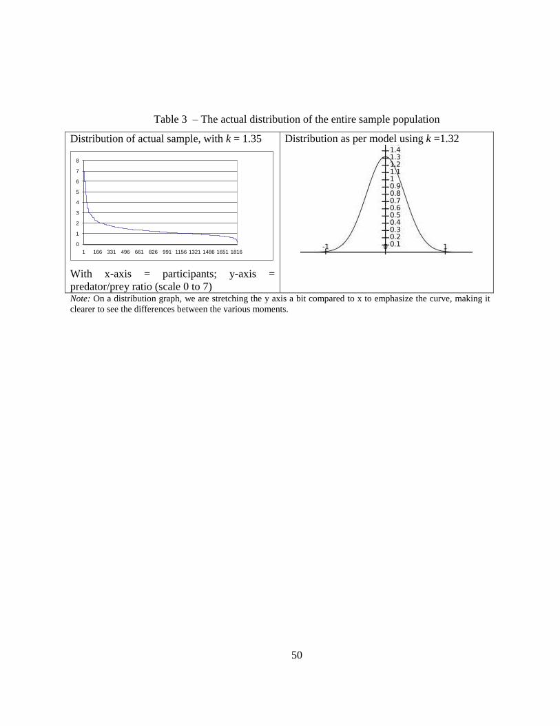
50

Table 3 – The actual distribution of the entire sample population

Distribution of actual sample, with k = 1.35

0

1

2

3

4

5

6

7

8

1 166 331 496 661 826 991 1156 1321 1486 1651 1816

With x-axis = participants; y-axis =

predator/prey ratio (scale 0 to 7)

Distribution as per model using k =1.32

Note: On a distribution graph, we are stretching the y axis a bit compared to x to emphasize the curve, making it

clearer to see the differences between the various moments.

51

Table 4 – Herding moment

Predatory distribution curve for the first

moment – herding): 2

1 0

2 1( )1

hx

kh

kf x e

Normal distribution curve (Gauss)

2

2

1

21( )

2

x

f x e

With the first part of the equation = k = 1.32

and σ2

= 1

52

Table 5 – Swarming moment

Predatory distribution curve for the second

moment – swarming): 2

1

2 2( )2

sx

ks

kf x e


2

2

1

21( )

2

x

f x e


divided by 2 and σ2

= 1

53

Table 6 – Limit moment

Predatory distribution curve for the limit

moment – just before self-

destruction/crash); at the limit of 2.3 of the

closed dynamic system: 2

limit1

2 2.3limit( )

2.3

x

kkf x e


2

2

1

21( )

2

x

f x e


divided by 2.3 and σ2

= 1

Note: Interestingly, the two curves are almost identical. The system limit is actually the closest representation of a Gaussian normal

distribution curve.

54

Table 7 – Stampeding moment

Predatory distribution curve for the third

moment – self-destruction or crash): 2

1

2 3( )

3

px

kp

kf x e


2

2

1

21( )

2

x

f x e


divided by 3 and σ2

= 1

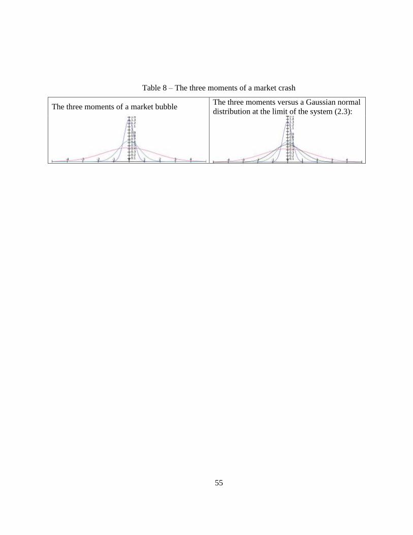
55

Table 8 – The three moments of a market crash

The three moments of a market bubble The three moments versus a Gaussian normal

distribution at the limit of the system (2.3):

56

Table 9 – The three moments of a market crash in sequence and payoffs

Initial state

(equilibrium)

Herding

(moment 1)

Swarming

(moment 2)

Stampeding

(moment 3)

1.15, 1.15 1.15, 1.15 2.30, 2.30 1.73, 0 1.15, 1.15 1.73, 0.58 0.58, 0.58 0, 2.30

1.15, 1.15 1.15, 1.15 0, 1.73 0, 0 0.58, 1.73 1.15, 1.15 2.30, 0 1.73, 1.73

Notes: This Table 9 is a sequential summary of Table 8 with, below the individual Figures, their respective payoff matrices. As can be seen, sellers and buyers maximize their positions by engaging and nourishing an increasingly toxic market environment.This exemplifies how an

otherwise rational market becomes over time an irrational one.

57

Table 10 – The Goods, the Bads and the Ugly

Quantity of Goods and Bads offered

Time0

+++

+++

QG

QB

Quantity of Goods and Bads offered

Time0

+++

+++

QG

QB

Herding Swarming Stampeding

Spread

58

Table 11 – Action and resting potentials and heteroscedasticity

Spread between Goods and Bads or

Heteroscedasticity of the moments’variances

Time0

+++

+++

Herding Swarming Stampeding

Type of market

Time

- - -

+++

+++

Action potential

Resting potential

Notes: On the left side, we see a representation of the change in variance in each of the three moments as they evolve over time. The right side of the above figure is its polarized rendition.

59

Figure 7 – HPI and Action-Resting potentials

0

0.1

0.2

0.3

0.4

0.5

0.6

1980 1985 1990 1995 2000 2005 2010 2015

Notes: 1981-1982;1990-1991; 2007-2009 - predatory mortgages31. We only display the major crises

that show a comparatively high peak. Source: own calculations.

31

https://fred.stlouisfed.org/. Accessed May 2016.

https://fred.stlouisfed.org/

60

Table 12 – Standard deviation predicted by the model and actual market results

Predicted by the

CMFP

1985

1993

2007-2009

Note: Recall the y axis is slightly overstretched compared to the x axis. Crises shown are: 1981-1982;1990-1991; and 2007-2009;

Source:FRED: https://fred.stlouisfed.org/series/GDP).

61

Figure 8 – Decision-to-invest formula and the stylized psychological model of financial

predation

ROI (reward)

Perceived

Risk/Fear

φ

Positivity bias

Ψ

QBadst+1

Decision to

invest (DI)

Notes: The fear to miss out on the opportunity to enter the market negatively impacts the

positivity bias (the belief things will go well) – obviously, the more the market agents fear, the

least likely they are to think positively of the market. As the positivity bias builds up, more Bads purchases are contemplated and, at the same time, more enthusiasm fuels the decision to invest.

As the investment turns out fruitful and returns on investments (ROI) increase, there are fewer

reason to fear. As fear lessens, the positivity bias gains in strength – blind trust is gaining

momentum.

An analysis of deviations in market bubble moments2 An analysis of deviations in market bubble...

Documents

Transcript of An analysis of deviations in market bubble moments2 An analysis of deviations in market bubble...