The Pennsylvania State University

The Graduate School

Department of Industrial and Manufacturing Engineering

EXTERNAL FAILURE COST ESTIMATION USING RELIABILITY MODELS:

AN ALTERNATIVE TO TAGUCHI’S LOSS FUNCTION

A Thesis in

Industrial Engineering

by

Jawad S. Hassan

2009 Jawad S. Hassan

Submitted in Partial Fulfillment

of the Requirements

for the Degree of

Master of Science

May 2009

ii

The thesis of Jawad S. Hassan was reviewed and approved* by the following:

M. Jeya Chandra

Professor of Industrial Engineering

Thesis Advisor

Susan H. Xu

Professor of Management Science and Supply Chain Management

Richard J. Koubek

Professor of Industrial Engineering

Head of the Department of Industrial and Manufacturing Engineering

*Signatures are on file in the Graduate School

iii

ABSTRACT

Taguchi’s quadratic loss function is used to capture the effect of nonconformance

to target values of quality characteristics in monetary values. Despite the merits of its

idea, there are major limitations of the quadratic loss function especially its use of a

proportionality constant that pools all the effects of external failure costs into a single

parameter. Researchers and practitioners alike agree that the proportionality constant of

the quadratic loss function is too simplistic in form and extremely difficult to estimate in

practice. That is why there have been many attempts to find alternatives to the quadratic

loss function.

In this study, an alternative to the quadratic loss function is presented by relating

the variance of the quality characteristic as well as the difference between the mean

setting and the target to the product’s reliability. Then, using warranty models, the

reliability is linked to external failure costs. This is shown for normally and beta

distributed N type, S type, and L type quality characteristics. A comprehensive

illustrative example is also presented that outlines the methodology of implementing

these models in real life problems.

iv

TABLE OF CONTENTS

LIST OF FIGURES ..................................................................................................... vi

LIST OF TABLES ....................................................................................................... vii

Chapter 1 Introduction ................................................................................................ 1

1.1 Problem Statement .......................................................................................... 1 1.1.1 Goal Post Mentality .............................................................................. 2 1.1.2 Taguchi’s Quadratic Loss Function ...................................................... 4

1.2 Literature Review: Alternatives to Taguchi’s Loss Function ......................... 6

1.2.1 Modification to the Quadratic Part of Taguchi’s Loss Function .......... 7

1.2.2 Dealing with the Proportionality Constant Part of Taguchi’s Loss

Function .................................................................................................. 12 1.3 Objectives ....................................................................................................... 17

Chapter 2 Model Formulation ..................................................................................... 18

2.1 Introduction ..................................................................................................... 18 2.2 Reliability Models .......................................................................................... 19

2.2.1 Nominal-the-Best (N Type) Quality Characteristic ............................. 20 2.2.2 Smaller-the-Better (S Type) Quality Characteristic ............................. 22 2.2.3 Larger-the-Better (L Type) Quality Characteristic ............................... 23

2.2.4 Relaxing the Normality Assumption of the Quality Characteristics .... 29

2.3 Determining Model Parameters using Maximum Likelihood Estimation

(MLE) ............................................................................................................ 32 2.4 Warranty Model Used to Estimate External Failure Costs ............................. 34

2.5 Numerical Computations ................................................................................ 36

Chapter 3 Model Validation and Numerical Example ................................................ 39

3.1 Introduction ..................................................................................................... 39 3.2 Model Validation ............................................................................................ 40

3.2.1 Normally Distributed S Type Quality Characteristic ........................... 40 3.2.2 Normally Distributed L Type Quality Characteristic ........................... 45 3.2.3 Beta Distributed Quality Characteristics .............................................. 48

3.3 Numerical Example ........................................................................................ 51

Chapter 4 Summary, Conclusions, and Future Research ............................................ 56

4.1 Summary and Conclusions ............................................................................. 56 4.2 Future Research .............................................................................................. 58

Bibliography ................................................................................................................ 59

v

Appendix A MATLAB Codes Used for Numerical Integration ................................. 62

A.1 Normally Distributed L type Quality Characteristic ...................................... 62

A.1.1 param_normal.m .................................................................................. 62 A.1.2 ltb_normal.m ........................................................................................ 63 A.1.3 adapquad.m .......................................................................................... 63

A.2 Beta Distributed N type Quality Characteristic ............................................. 64 A.2.1 param_beta.m ...................................................................................... 65

A.2.2 beta1.m ................................................................................................ 65

vi

LIST OF FIGURES

Figure 1.1: Goal post mentality ................................................................................... 3

Figure 2.1: % error – in using approximations of mean and standard deviation of

1 X and mean of 21 X – vs. the ratio ....................................................... 27

Figure 3.1: Effect of variation in x on conditional reliability for a normally

distributed S type quality characteristic ................................................................ 41

Figure 3.2: Effect of variation in mean on unconditional reliability for a normally

distributed S type quality characteristic ( 0.1 ) ............................................... 42

Figure 3.3: Effect of variation in standard deviation on unconditional reliability

for a normally distributed S type quality characteristic ( 1 ) ........................... 43

Figure 3.4: Effect of variation in x on conditional reliability for a normally

distributed L type quality characteristic ............................................................... 45

Figure 3.5: Effect of variation in mean on unconditional reliability for a normally

distributed L type quality characteristic ( 2.236 ) ........................................... 46

Figure 3.6: Effect of variation in standard deviation on unconditional reliability

for a normally distributed L type quality characteristic ( 50 ) ........................ 47

Figure 3.7: Effect of variation in x on conditional reliability for a beta distributed

S type quality characteristic .................................................................................. 49

Figure 3.8: Effect of variation in mean on unconditional reliability for a beta

distributed S type quality characteristic ( 0.2 , 1LL , and

3UL ) ........................................................................................................... 50

Figure 3.9: Effect of variation in standard deviation on unconditional reliability

for a beta distributed S type quality characteristic ( 1 , 0LL , and

4UL ) ................................................................................................................. 51

Figure 3.10: Numerical and approximate LR t solutions of the numerical

example ................................................................................................................. 54

vii

LIST OF TABLES

Table 3.1: Effect of on the accuracy of the approximate unconditional

reliability function of an L type quality characteristic .......................................... 48

Table 3.2: Sample data set of failure times of an L type quality characteristic ........... 52

Table 3.10: Calculated values of the numerical and approximate LR t solutions

of the numerical example including the % error between the two solutions ........ 53

Chapter 1

Introduction

1.1 Problem Statement

One of the well-established principles in the field of quality control when it comes

to evaluating the quality of a product or service is that higher quality is achieved when

the product or service conforms to its ideal or target specifications. Consequently, one of

the definitions of quality besides “fitness for use” or “satisfying customer’s

requirements” is simply “conformance to requirements” (Chandra, 2001).

Due to the inherent variability in, for instance, manufacturing processes, it is

virtually impossible to produce products that always match their ideal targets perfectly.

That is why every product dimension and characteristic of interest has to have tolerance

limits around its ideal or target value. Subsequently, with these tolerance limits, the

product dimension or characteristic is considered to be satisfactory if its value falls within

the specified tolerance limits. If, on the other hand, the value of the product dimension or

characteristic falls outside the tolerance limits, the dimension or characteristic would be

considered unsatisfactory and it must be reworked or scraped. Moreover, it is worth

mentioning that the natural variability in any quality characteristic of a product, i.e. its

variance, is a signature of the process itself while the mean of the quality characteristic

depends upon the process setting (Chandra, 2001).

2

1.1.1 Goal Post Mentality

The costs associated with a certain product could be divided into two main

categories. The first category is the costs acquired by the manufacturer before the product

is shipped. These costs are related to the product’s manufacturing process, such as, cost

of raw materials, personnel, product rework and scrap, etc. The second category is the

quality-loss costs acquired by the manufacturer, customer, and society after the product is

shipped. These costs are related to warranty costs, customer complaints and

dissatisfaction, etc. (Taguchi et al., 1990).

Before the introduction of the revolutionary idea of a loss function by the

renowned Dr. Genichi Taguchi, the common belief was that if a product or service falls

within its tolerance limits, then there would not be any other costs associated with that

product or service to its manufacturer, provider, consumer, or society in general. This

means that if two products with all of their quality characteristics falling within the

specified tolerances, even if one was always on target while the other was always barely

within the tolerances, these two products would be practically identical in their

appearance, functionality, reliability, costs to society, etc. This way of thinking, i.e.

pass/fail or in-spec/out-of-spec (Taguchi et al., 1990), is often referred to as the goal post

mentality (Blue, 2001). The goal post mentality is presented in figure 1. Here, LSL and

USL are the upper and lower specification limits (tolerances), respectively.

From figure 1, it can be seen that the goal post mentally representation of a

product’s losses completely ignores the costs associated with poor quality incurred after a

product is shipped. Only factory losses, including internal failure costs, are considered.

3

Figure 1.1: Goal post mentality

The goal post mentally has been proven to be inadequate in providing accurate

representation of the costs associated with nonconformance to targets or ideal values.

One of the classic examples of this inadequacy of the goal post mentally is the Ford

versus Mazda case of the 1980’s discussed by Taguchi et al. (1990).

According to Taguchi et al. (1990), Ford, the car manufacturing company, used to

import some of the transmissions needed for one of its cars that were being sold in the

United States from the Japanese company Mazda (25% of Mazda was owned by Ford).

After a while, it became clear that most of the transmission warranty costs and customer

complaints were generated by the transmissions produced by Ford. Surprisingly, after a

thorough investigation, it has been found that both the Mazda-made and Ford-made

transmissions had parts that were all made according to the specified tolerances.

However, the Ford-made transmissions’ parts had more variability while the Mazda-

made transmissions’ parts “betrayed no variability at all from targets” (Taguchi et al.,

4

1990). The authors indicated that this is a clear example of how the zero-defects

definition of quality failed to capture all the costs associated with the product. That is

because, even though the quality characteristics were all within the specification limits,

when these quality characteristics were not close to their corresponding ideal values and

the different parts of the transmission were put together randomly, the effects of the

nonconformance to specifications were amplified. This resulted in greater friction and

vibration which, in turn, caused excessive noise and shorter transmission life (Taguchi et

al., 1990).

Again, from the discussion above, it is clear that the goal post mentality does not

provide an accurate representation of the costs associated with a product. For this reason,

Taguchi’s quadratic loss function has been developed.

1.1.2 Taguchi’s Quadratic Loss Function

Maghsoodloo et al. (2004) suggested that one of the most significant contributions

of Taguchi’s work in the quality engineering field is his quadratic loss function. That is

because it provided a new definition for quality and a new vision for what needs to be

sought after in improving the quality of a product or a process. Moreover, it provided a

tool for measuring the monetary cost of not adhering to the principles of being on target

and minimizing variability.

The most widely used form of Taguchi’s loss function is the quadratic form that is

arrived at by employing the Taylor series expansion and ignoring higher order terms. The

final form of the loss function for a nominal-the-best (N type) quality characteristic X is:

5

2

0( ) ( ) ,L X k X X LSL X USL (1.1)

where, k is a constant that defines the monetary cost of a unit deviation from the target

0X . Also, LSL and USL are the lower and upper specification limits, respectively.

Obviously, if X LSL or X USL , the product would not be shipped and, technically,

the external failure costs are assumed to be zero. However, the manufacturer would incur

scrap or rework losses (internal failure costs). The quadratic loss function in its general

form is established for an N type quality characteristic as shown in equation (1.1) with

symmetric losses at the LSL and USL . However, this has been extended to the larger-

the-better (L type), i.e. 2( ) /L X k X X LSL , and smaller-the-better (S type), i.e.

2( )L X k X X USL , quality characteristics as well. Moreover, this formulation has

been further extended to the cases of asymmetrical losses at the LSL and USL as shown

in equation (1.2) for an N type quality characteristic (Chandra, 2001):

2

1 0 0

2

2 0 0

( )k X X if LSL X X

L Xk X X if X X USL

(1.2)

Again, in equation (1.2), 1k and 2k are the monetary values of loss to society for

underestimating and overestimating the target 0X , respectively.

The quadratic loss function has been criticized and deemed inappropriate, in

certain situations, by many researchers including Schneider et al. (1995) who suggested

that it is highly possible for the loss incurred due to the deviation of the quality

characteristic from its target to be non-quadratic. Moreover, the authors also suggested

that even if an ideal target could be determined, which in on itself is not always possible,

6

“producing exactly at target may be unnecessarily costly and thus increase the price of

the product” (Schneider et al., 1995).

Another major criticism of the quadratic loss function has been the use of the

proportionality constant k in its formulation in which it gives a pooled representation of

all the external failure costs of the product’s deviation from target. This is believed by

many researchers to be too simplistic mathematically and extremely difficult to estimate

practically.

To Taguchi’s credit, however, it is mentioned in Taguchi et al. (1990) that the

quadratic loss function (QLF) “is a simple approximation, to be sure, not a law of

nature”. The authors continue to say that “actual field data cannot be expected to

vindicate QLF precisely, and if your corporation has a more exacting way of tracking the

costs of product failure, use it” (Taguchi et al., 1990).

Therefore, mainly due to the limitations of the simple quadratic loss function,

researchers have come up with a number of alternatives to Taguchi’s loss function with

the objective of eliminating or, at least, reducing the effects of the limitations mentioned

above.

The following section presents a literature review of studies that attempted to

come up with alternatives to the Taguchi quadratic loss function.

1.2 Literature Review: Alternatives to Taguchi’s Loss Function

In this section, initially, the studies that address and modify the quadratic part, i.e.

2

0X X , of Taguchi’s loss function are presented. Then, the studies that tackle the

7

issue of the proportionality constant k and more drastically alter the quadratic loss

function are presented. The research in this thesis is more closely related to those studies

that take on the issue of the proportionality constant k .

1.2.1 Modification to the Quadratic Part of Taguchi’s Loss Function

Li (2005) introduced a truncated asymmetric linear loss function as an alternative

to the quadratic loss function. He suggested that, in many industrial situations, the linear

loss function provides a better representation of the external failure costs especially if the

costs are unequal when the target is overestimated or underestimated. The main objective

of the study was to find a methodical and logical way of defining the target of a process

mean. Li (2005) argued that often in practice, the way to define the target for a quality

characteristic that has asymmetric losses would be to either set the target at the midpoint

between the lower and upper specification limits or to use the length of the shorter

specification limit as the tolerance for both sides. Neither of these traditional methods is

believed to be appropriate. In this paper, it was found that the optimal process mean

setting was slightly different than what is usually determined to be in practice.

In order to find the optimal target value for the mean, the truncated asymmetric

linear loss function has been used. The format of the loss function was (Li, 2005):

1

1

2

2

( )

A if y LSL

k y m if LSL y mL y

k y m if m y USL

A if y USL

(1.3)

8

where, LSL is the lower specification limit, USL is the upper specification limit,

1 1A k m LSL , and 2 2A k USL m . Using the expected value of the loss function,

Li (2005) constructed a table that shows how the optimal value of the target mean can be

specified using three main parameters. These parameters were: 1) 1 2kR k k ; 2)

1 2AR A A ; and 3) the process capability ratio, i.e. 6pC USL LSL . Thus, once

the three parameters are specified, it is a simple task to find the optimal target for the

mean of the quality characteristic.

Finally, since the main parameters affecting the optimal value of the target were

kR , AR , and (since pC is a function of provided that LSL and USL were already

specified), a sensitivity analysis was conducted to investigate the effects of

misrepresenting the parameters kR and AR as well as variations in . For the parameter

, it was found that as the standard deviation increased, the larger the difference was

between the optimal target and the target found using traditional methods.

Spiring (1993) was the first to introduce the idea of the reflected-normal loss

function. In this method, the bell-shaped Gaussian curve of a normal distribution is

inverted upside down and defined as a loss function with its minimum occurring at the

specified target of the quality characteristic. This reflected-normal loss function has two

main parameters. The first one is K which determines the maximum cost incurred due to

the deviation of the quality characteristic from its target and the second one is a shape

parameter that determines how concentrated (wide or narrow) the V-shaped curve is.

Spiring (1993) stated that, because of its compact form and its shape parameter,

the reflected-normal loss function is intuitively more appealing and more flexible than the

9

quadratic loss function. Moreover, the author mentioned that the reflected-normal loss

function can easily be extended to the case where the maximum loss values are not equal

at the upper and lower specification limits. To account for this asymmetric situation, the

author stated that “the symmetric results are also extendible to the asymmetric case using

piecewise fits on each side of the target” (Spiring, 1993). Simple numerical examples

were also given in the paper to illustrate the use of univariate (symmetric and

asymmetric) and bivariate reflected-normal loss functions and compare them to the

quadratic loss function.

One of the major differences that can be noted between the quadratic loss function

and the inverted-normal loss function is the fact that both have flat minimums with the

quadratic loss function being the flatter of the two. This suggests that very small

deviations are not as costly as larger deviations. However, in the case of the quadratic

loss function, this fact is true all the way to the specification limits while, in the case of

the inverted-normal loss function, the loss tends to asymptotically level off and be less

drastic as the deviation of the quality characteristic gets closer to the maximum loss value

at the upper and lower specification limits. Even though the author mentioned this

difference between the inverted-normal loss function and the quadratic loss function, he

did not provide any discussion about whether either behavior is superior to the other

based on common real life problems or even intuition.

Spiring et al. (1998) continued on the same path as that of Spiring (1993) by

investigating other continuous probability density function distributions that can be

inverted to provide alternative representations of loss functions. Spiring et al. (1998),

once again, started by presenting the inverted-normal loss function and derived its

10

expectation as in Spiring (1993). This time, however, different process distributions of

the quality characteristic were considered besides the normal distribution. That is, the

expected loss of the inverted-normal loss function was examined under the assumption

that the underlying distribution of the process characteristic was normal, gamma, or

uniform. The authors stated that it is fairly straightforward to come up with different loss

functions by changing the parameters of the inverted-normal loss function to get

reasonable representation of the loss incurred by the process when the underlying

distribution of the process is normal. However, if the underlying distribution of the

quality characteristic is not normal, finding the expected loss function of the inverted-

normal loss function can be difficult or even impossible.

The paper then mentioned that since it is very likely in many applications for the

loss function to be asymmetric, using an inverted-gamma distribution would be much

more practical than the naturally symmetric inverted-normal loss function because of the

inherent asymmetric nature of the gamma distribution. This in turn widens the class of

loss functions that use inverted probability density function distributions to represent the

cost of deviation from a specified target for the quality characteristic. Again, it has been

seen in Spiring (1993) how to use the reflected-normal loss function to represent

asymmetric loss functions. However, that method required fitting two halves of the

inverted-normal loss function to represent the asymmetric nature. In the inverted-gamma

loss function, however, it is one continuous function. Finally, an appendix was provided

at the end of the paper by Spiring et al. (1998) in which the expected loss function of the

inverted-gamma loss function has been derived for different underlying process

distributions.

11

Another similar class of loss functions was then introduced in Spiring et al. (1998)

in which an inverted-lambda loss function was presented. This was based on Tukey’s

symmetric lambda distribution. Again, similar to the inverted-normal loss function, the

inverted lambda loss function was found to be symmetric. It behaved very similar to the

inverted-normal loss function when its parameter was less than 1. However, when

1 2 , the maximum loss was found to occur at the target of the quality characteristic.

This is obviously the exact opposite to what actually happens. Therefore, it is important

to be cautious when using the inverted-lambda loss function.

Leung et al. (2002) presented a new class of inverted loss functions. This was

based on the probability density function of the beta distribution, hence the name the

inverted-beta loss function. In this paper, the authors argued that the loss function based

on the beta distribution is the most flexible of all other distribution-based loss functions,

such as, the inverted-normal and inverted-gamma distributions.

The inverted-beta loss function’s shape can be altered and modified depending on

the application or problem at hand by changing the values of its parameters and .

The optimal target value T was a function of these two parameters only. This was true

only when and were greater than one since, for and values less than one, the

resulting shape of the loss function was not unimodal. This problem was reported in the

paper as the only limitation of using the inverted-beta loss function. Moreover, since the

optimal target value T was only a function of and , it was found that for a fixed

value of T , “as increases, will increase. Alternatively, when keeping fixed and

increasing T , will decrease” (Leung et al. (2002).

12

In this paper, Leung et al. (2002) presented different scenarios and curve shapes

that would be achieved for the inverted-beta loss function as the parameters and

were varied. It was found that, in order to have a symmetric loss function, the values of

and had to be equal. Unequal values of and resulted in curve shapes that

were skewed one way or the other. Moreover, the case of asymmetrical loss functions

was considered. There were two methods to deal with this issue. Either two different

inverted-beta loss functions were fitted to each side of the target or a single inverted-beta

loss function was used and the parameters and were tweaked and changed until a

good representation of the quality characteristic’s loss function was achieved.

All of the studies presented in this section were concerned with the quadratic part

of Taguchi’s loss function. However, no attempt was made to redefine the proportionality

constant k of the quadratic loss function or alter the way it was estimated. Consequently,

the significance of these studies as alternatives to Taguchi’s quadratic loss function was

limited.

1.2.2 Dealing with the Proportionality Constant Part of Taguchi’s Loss Function

Deleveaux (1997) was the first to introduce the idea of capturing the amount of

external failure costs incurred from a product based on its quality characteristic’s

variance and mean setting. This was achieved by first relating the quality characteristic’s

variance and mean setting to the product’s reliability. Then, by incorporating the

product’s reliability into warranty models, external failure costs were linked to the

variance and mean setting. Thus, an alternative to Taguchi’s loss function was developed

13

in which the effect of high variance and deviation from targets were related to liability

and warranty costs. This, similar to Taguchi’s loss function, provides a tool that aids

decision makers to assess the effect of variance and conformance to targets in monetary

values.

The reliability model that was used by Deleveaux (1997) was a bi-variate Weibull

proportional-hazard function in which the failure rate of the product was a function of

variance and mean setting as well as time. A convenient way in which variance and mean

setting were incorporated in this reliability model was by combining them into a

capability index for individual sample observations using a similar definition used for the

Cpm capability index. The capability index for an individual item x from a sample of n

items was defined as (Deleveaux, 1997):

0 0

2 2

0 0

min ,3 3

x LSL USL xc

x x x x

(1.4)

where, 0x , USL and LSL are the target value, upper and lower specification limits,

respectively. Then, the conditional reliability function was found to be (Deleveaux,

1997):

2| exp expR t x t Bc (1.5)

where, x is the observed value of the quality characteristic of an item, t is time to

failure, is the shape parameter, B is a constant coefficient, and c is the individual

capability index defined in equation (1.4). The next step after developing an expression

for the reliability function was to use Bayesian statistics to estimate the parameters in the

14

reliability function, namely, and B . Then, estimates of the external failure costs of

items were calculated using warranty models and other indirect costs.

The advantage of Deleveaux’s (1997) approach is obvious and is backed up by

numerous case studies. Instead of treating the failure time of different items of the same

product to be the same, a distinction is made among the items based on conformance to

target values in which the items with closer values to targets are expected to be more

reliable. Having said that, one of the limitations of this model was that finding the

unconditional reliability function based on equation (1.5) was very complicated and was

not pursued by Deleveaux (1997). Instead, bounds on individual reliabilities were

developed by employing Jensen’s inequality. Another limitation of the model was the use

of capability indices which are developed with the assumption that the underlying

distribution of the quality characteristic is normal. Thus, extending this reliability model

to non-normally distributed quality characteristics is a problem.

An application of the models developed by Deleveaux (1997) can be found in the

work by Lee (2008) who used these models to estimate warranty costs, which were part

of the total cost model of return on investment in quality improvement projects.

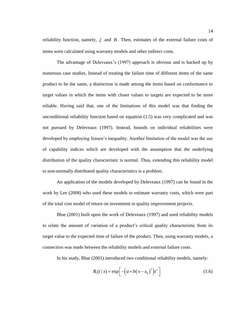
Blue (2001) built upon the work of Deleveaux (1997) and used reliability models

to relate the amount of variation of a product’s critical quality characteristic from its

target value to the expected time of failure of the product. Then, using warranty models, a

connection was made between the reliability models and external failure costs.

In his study, Blue (2001) introduced two conditional reliability models, namely:

2

1 0( | ) exp cR t x a b x x t

(1.6)

15

and,

2 2

2 0( | ) exp cR t x a b x x d t

(1.7)

where, x is the observed value of an N type quality characteristic, t is the time to failure,

2 is the population variance of the quality characteristic, and 0x is the target value.

Moreover, a , b , and c are scaling constants used to provide enough flexibility in the

model, allowing it to better fit data sets of real life problems. Using the models in

equations (1.6) and (1.7), closed-form expressions for the unconditional reliability

functions were developed by taking the expected values of the conditional reliability

functions with the assumption that the underlying quality characteristic was normally

distributed. Thus, the unconditional reliability was directly related to the process mean

and variance in these expressions. Then, these unconditional reliability functions were

used along with a common warranty model to estimate the external failure costs.

It is to be noted that the first reliability model given by equation (1.6) is more

realistic than the second reliability model given by equation (1.7). That is because the

first reliability model relates the reliability of a system or product to the deviation from

target and time. Therefore, as the deviation of the quality characteristic from its target

value increases, the reliability of the product or system decreases. Also, as time passes,

the reliability of the product or system decreases as well. The second reliability model, on

the other hand, even though it captures the same effects of deviation from target and time

on reliability as in the first reliability model, it also relates the reliability of the product or

system to the population variance by adding the term 2d into the reliability model. This

extra term that relates the conditional reliability of a product or system to the population

16

variance is questionable. That is because, for instance, if there were two identical

products with their quality characteristics matching exactly to the target value and each

other, they both ought to be equally perfect and incur no quality related costs, even if one

was produced by a process with high variance and the other by a process with low

variance.

An application of the models developed by Blue (2001) can be found in the work

by Nocerito (2002) who used these models to estimate the effect of reducing the variance

of a product on external failure costs by worker training programs.

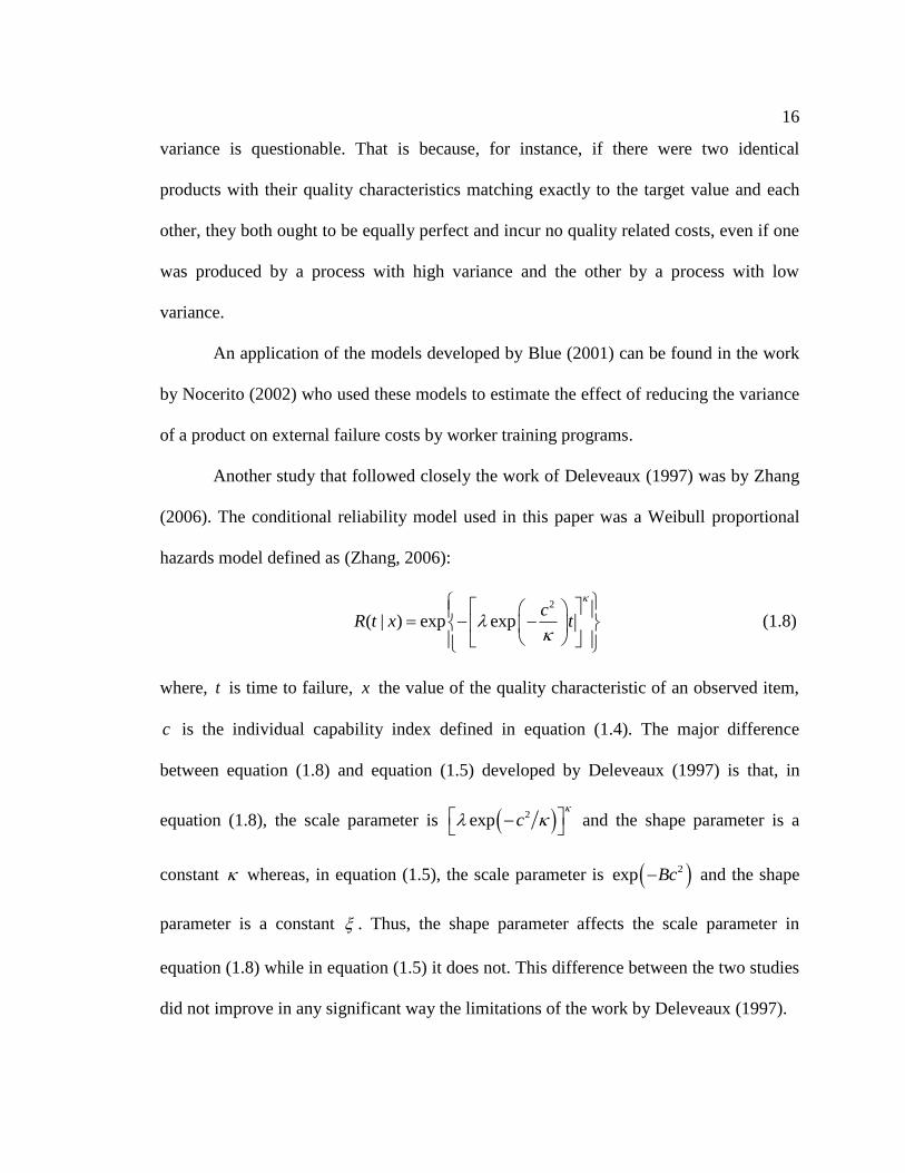
Another study that followed closely the work of Deleveaux (1997) was by Zhang

(2006). The conditional reliability model used in this paper was a Weibull proportional

hazards model defined as (Zhang, 2006):

2

( | ) exp expc

R t x t

(1.8)

where, t is time to failure, x the value of the quality characteristic of an observed item,

c is the individual capability index defined in equation (1.4). The major difference

between equation (1.8) and equation (1.5) developed by Deleveaux (1997) is that, in

equation (1.8), the scale parameter is 2exp c

and the shape parameter is a

constant whereas, in equation (1.5), the scale parameter is 2exp Bc and the shape

parameter is a constant . Thus, the shape parameter affects the scale parameter in

equation (1.8) while in equation (1.5) it does not. This difference between the two studies

did not improve in any significant way the limitations of the work by Deleveaux (1997).

17

1.3 Objectives

From the literature review, it was concluded that the first reliability model by

Blue (2001), i.e. equation (1.6), had the most potential for further study. That is because

it captured the effect of deviation from target on the reliability of the product while

containing enough flexibility to fit real life data sets. Furthermore, closed-form

expressions were possible to be developed for the unconditional reliability function

which made the model especially valuable in estimating the expected reliability of a

population of products.

Thus, in this study, the first reliability model developed by Blue (2001), which

was only for an N type quality characteristic, is extended to include quality characteristics

of the S type and L type. Moreover, the normality assumption of the underlying process

is relaxed and, instead, a more flexible distribution, namely, the beta distribution, is used

as the distribution of the quality characteristic. Then, following similar steps as in the

works by Deleveaux (1997) and Blue (2001), a simple warranty model is used to estimate

external failure costs using the reliability models. Finally, after validating the reliability

models, a numerical example is presented underlining the procedure of implementing the

developed models in real life problems.

18

Chapter 2

Model Formulation

2.1 Introduction

From the literature review, it was concluded that even though Taguchi’s loss

function was conceptually an extremely powerful tool used to express external failure

costs in monetary values, the formulation of the loss function was too simplistic and its

proportionality constant was difficult to estimate. That is why there have been a

significant number of attempts to develop alternatives to Taguchi’s loss function.

This thesis is based on the studies by Deleveaux (1997) and Blue (2001). The

main idea behind these two studies was to employ reliability models in order to relate the

deviation of the quality characteristic of a system or product from its target value to its

reliability. Then, using warranty models, the reliability of the system or product was

presented in monetary value and thereby establishing a connection between deviation

from target and the associated warranty cost.

In this chapter, reliability models that relate the reliability of a product or system

to the mean and variance of its quality characteristic are first introduced. Then, the

method of maximum likelihood estimation (MLE) is presented which is used to estimate

the scaling parameters of the reliability models. After that, the warranty model used to

estimate external failure costs is shown. Finally, the numerical computations used to

calculate some of the reliability functions are described.

19

2.2 Reliability Models

A formal definition of reliability is given by Leemis (2009) and it states that “the

reliability of an item is the probability that it will adequately perform its specified

purpose for a specified period of time under specified environmental conditions”. Thus, it

follows from the definition that the main random variable of traditional reliability models

is time to failure T . The distribution of a continuous nonnegative random variable T can

be uniquely represented by the probability density function f t , cumulative distribution

function F t , reliability function R t , and the hazard rate function h t among a few

other representations. These functions are related to each other as follows:

1R t F t (2.1)

d R t

f tdt

(2.2)

f th t

R t (2.3)

In this section, reliability models for the N type, S type, and L type quality

characteristics are introduced. First, the quality characteristics are assumed to be normal.

Then, the normality assumption is relaxed and beta distributed quality characteristics are

considered instead. In each case, development of expressions of the reliability function

R t , probability density function f t , and the hazard rate function h t are presented

in detail.

20

2.2.1 Nominal-the-Best (N Type) Quality Characteristic

The N type quality characteristic is the case when the quality characteristic of a

product or service requires conformance to the target value as much as possible and any

deviation from the target value, from either side, results in lower quality and the

incurrence of some quality cost (Taguchi et al., 1989). Thus, this type of quality

characteristic requires the specification of both upper and lower specification limits (USL

and LSL).

The conditional reliability model used in this study for a quality characteristic of

the N type was exactly the same as the first model developed by Blue (2001), namely,

2

0( | ) exp c

NR t x a b x x t

(2.4)

where, x is the observed value of the quality characteristic, t is the time to failure, and

0x is the target value. Moreover, a , b , and c are scaling constants used to provide

enough flexibility in the model, allowing it to better fit data sets of real life problems.

The most important characteristic of the conditional reliability model given in

equation (2.4) is that the reliability decreases as the deviation of the quality characteristic

from its target value increases. This effect is captured by the term 2

0x x in the model.

Moreover, it follows from equation (2.4) that the probability density function and the

hazard rate function are (Blue, 2001):

2 21

0 0( | ) expc c

Nf t x a b x x ct a b x x t

(2.5)

2 1

0( | ) c

Nh t x a b x x ct (2.6)

21

The unconditional reliability function NR t was then developed by taking the

expected value of the conditional reliability function given in equation (2.4). In order to

be able to take the expected value of the conditional reliability function, the underlying

distribution of the quality characteristic X had to be assumed. Since the majority of

quality characteristics of products and systems in practice are normally distributed, the

normal distribution was used to determine the unconditional reliability function NR t as

follows (Blue, 2001):

2

2

0 22

1( ) exp exp

22

c

N

xR t a b x x t dx

2

0

22

1exp

1 21 2

c

N cc

b xR t a t

b tb t

(2.7)

where, and 2 are the mean and variance of the normally distributed quality

characteristic X . It is clear from equation (2.7) that the unconditional reliability NR t

decreases as the deviation between the population mean of the quality characteristic and

its target value increases. The effect of the variance on NR t is less obvious since the

variance appears more than once in equation (2.7).

Likewise, the unconditional probability density function and the unconditional

hazard rate function were found to be (Blue, 2001):

2 22 1

0 0

22 222exp

1 2 1 21 21 2

cc

N c ccc

b x b xb ctf t a a t

b t b tb tb t

(2.8)

22

220 1

22 21 2 1 2

c

N c c

b xbh t a ct

b t b t

(2.9)

2.2.2 Smaller-the-Better (S Type) Quality Characteristic

The S type quality characteristic is the case when it is desirable for the quality

characteristic of a product or service to be as small as possible. Thus, the target value in

this case is set to zero and any other value of the quality characteristic results in acquiring

additional quality costs (Taguchi et al., 1989). Consequently, the S type quality

characteristic only requires an upper specification limit (USL).

For the case of a quality characteristic of the S type, similar formulations have

been followed as in section 2.2.1 for the N type quality characteristic. The only difference

between the N type and S type quality characteristics is that the target value is set to zero

for the S type quality characteristic. Thus, the conditional reliability function, the

probability density function and the hazard rate function are found to be:

2( | ) exp c

SR t x a bx t

(2.10)

2 1 2( | ) expc c

Sf t x a bx ct a bx t

(2.11)

2 1( | ) c

Sh t x a bx ct (2.12)

where, x is the observed value of the quality characteristic and t is the time to failure.

Further, a , b , and c are scaling parameters which are constants. Again, from equation

(2.10), it can be seen that the conditional reliability decreases as x increases. Moreover,

the unconditional reliability is found by taking the expected value of the conditional

23

reliability model with the assumption that the underlying distribution of the quality

characteristic is normal. Thus, the unconditional reliability is determined to be:

2

22

1exp

1 21 2

c

S cc

bR t a t

b tb t

(2.13)

where, and 2 are the mean and variance of the normally distributed quality

characteristic X . Also, the unconditional probability density function and the

unconditional hazard rate function are:

2 2 1 2

22 222exp

1 2 1 21 21 2

cc

S c ccc

b b ct bf t a a t

b t b tb tb t

(2.14)

2 21

22 21 2 1 2

c

S c c

b bh t a ct

b t b t

(2.15)

2.2.3 Larger-the-Better (L Type) Quality Characteristic

The L type quality characteristic is the exact opposite of the S type quality

characteristic. That is, when it is desirable for the quality characteristic of a product or

service to be as large as possible, then it is called an L type quality characteristic. Thus,

the target value in this case is ideally equal to infinity and any other value of the quality

characteristic results in acquiring additional quality costs (Taguchi et al., 1989).

Consequently, the L type quality characteristic only requires a lower specification limit

(LSL). It is common in practice, however, to use the inverse of the quality characteristic,

which is of the S type, whenever it is necessary since its target value is zero instead of

24

infinity. This makes the quality characteristic easier to handle mathematically (Chandra,

2001). Therefore, the conditional reliability function, the probability density function and

the hazard rate function for the L type quality characteristic are found to be:

2

( | ) exp c

L

bR t x a t

x

(2.16)

1

2 2( | ) expc c

L

b bf t x a ct a t

x x

(2.17)

1

2( | ) c

L

bh t x a ct

x

(2.18)

where, x is the observed value of the quality characteristic and t is the time to failure.

Also, a , b , and c are scaling parameters which are constants. As it can be seen from

equation (2.16), the conditional reliability decreases as x decreases, which is what is

expected from an L type quality characteristic.

In order to find the unconditional reliability expression for the L type quality

characteristic, similar to the N type and S type cases, the distribution of the quality

characteristic is assumed to be normal. Then, the expected value of the conditional

reliability is found as follows:

2

2 22

1( ) exp exp

22

c

L

xbR t a t dx

x

(2.19)

where, and 2 are the mean and variance of the normally distributed quality

characteristic X .

It is to be noted that there is no simple exact closed-form expression for the

integral in equation (2.19). This integral can be evaluated to the desired accuracy by

25

using numerical integration. This method is shown in section (2.5). On the other hand, it

is still possible to find an approximate solution to the unconditional reliability of the L

type quality characteristic by using the same expression found for the unconditional

reliability for the S type quality characteristic, i.e. equations (2.13). However, in order to

be able to do that, the inverse of the quality characteristic, namely 1 X , has to be used as

the desired variable instead of the quality characteristic itself X since 1 X would be an

S type quality characteristic. This in turn can only be achieved if an assumption could be

made about the distribution of the inverse of the quality characteristic and expressions for

the mean and variance of 1 X could be developed in terms of the mean and variance of

the original quality characteristic X .

Using Taylor series expansion at X and ignoring high order terms, an

approximate expression for the expected value of 1 X is found as follows:

2

2 3

1 1 1 1X X

X

2

2 3

0

1 1 1 1E E X E X

X

2

3

1 1E

X

(2.20)

In addition, using the same methodology, an approximate expression for the

expected value of 21 X is found as follows:

2

2 2 3 4

1 1 2 3X X

X

26

2

2 2 3 4

0

1 1 2 3E E X E X

X

2

2 2 4

1 1 3E

X

(2.21)

Thus, the variance of the inverse of the quality characteristic is given by:

2

2

1 1 1var E E

X X X

22 2

2 4 3

2 2 4

2 4 2 4 6

1 1 3 1var

1 3 1 2

X

2 4

4 6

1var

X

(2.22)

It is important to realize that the expressions given in equations (2.20) and (2.22)

for the mean and variance of the inverse of the quality characteristic are only

approximations. That is, for a normally distributed quality characteristic X with mean

and variance 2 , the mean and variance of 1 X can be reasonably approximated by

equations (2.20) and (2.22), respectively, if the ratio is much greater than one.

Figure 2.1 presents the effect of the ratio on the percentage errors between

real values of the means of 1 X and 21 X as well as the standard deviation of 1 X

compared to their approximations given by equations (2.20) to (2.22). The “real” values

of the means of 1 X and 21 X as well as the standard deviation of 1 X were found

from a randomly generated and normally distributed data sets of large sizes (N = 1600

27

points). The inverse and the inverse squared of these data points were calculated and their

sample means and sample standard deviations were recorded and used as the real values.

The percentage error was defined as the difference between the real and approximate

values, divided by the real value, and multiplied by 100%.

Figure 2.1: % error – in using approximations of mean and standard deviation of 1 X and

mean of 21 X – vs. the ratio

As it can be seen from figure 2.1, as long as the ratio is greater than about

10, the approximations given by equations (2.20) to (2.22) are within 5% error, which

makes them very reasonable for most practical purposes. Moreover, since it is very

common for the ratio to be large especially when dealing with L type quality

characteristics, the approximations given by equations (2.20) and (2.22) are expected to

0

5

10

15

20

25

30

0 5 10 15 20 25

mean 1/x

std 1/x

mean 1/x 2̂

% E

rror

Mean of 1 X

Std. dev. of 1 X

Mean of 21 X

28

produce accurate results when used as the mean and variance of 1 X in the equation for

the unconditional reliability of an S type quality characteristic (equation (2.13)). Thus,

the resulting approximate expression for the unconditional reliability of an L type quality

characteristic is:

22

3

2 42 4

4 64 6

1

1exp

1 21 2

c

L

cc

b

R t a t

b tb t

(2.23)

where, and 2 are the mean and variance of the normally distributed quality

characteristic X . The results from this approximate expression of the unconditional

reliability and results of the exact numerically integrated expression given by equation

(2.19) are compared in chapter 3 when model validation is presented.

The unconditional probability density function and the unconditional hazard rate

function are then:

22 4 2

4 6 3 1

22 4 2 42 4

4 6 4 64 6

1

1 2 1 21 2

c

L

c cc

b bct

f t a

b t b tb t

22

3

2 4

4 6

1

* exp

1 2

c

c

b

a t

b t

(2.24)

29

22 4 2

4 6 3

1

22 42 4

4 64 6

1

1 2 1 2

c

L

cc

b b

h t a ct

b t b t

(2.25)

2.2.4 Relaxing the Normality Assumption of the Quality Characteristics

Even though it is quite common in many practical applications for the quality

characteristic of a product or system to be normally distributed, in some cases, the

normality assumption does not hold. For instance, if the quality characteristic’s

distribution is skewed or bounded, the assumption of normality, which is inherently

symmetric and unbounded, will not be appropriate. That is why among the three types of

quality characteristics considered in this study, i.e. N type, S type, and L type quality

characteristics, the normality assumption is especially questionable in the case of an S

type quality characteristic since the S type quality characteristic is bounded by zero.

Therefore, besides the normal distribution, the beta distribution is also considered in this

study as the quality characteristic’s distribution in the derivation of the unconditional

reliability functions.

The beta distribution is a much more flexible distribution than the normal

distribution since it can be fitted to skewed and bounded data sets. There are four main

parameters of the beta distribution. These parameters are the lower and upper limits LL

and UL , respectively, which determine the range of the values of the quality

30

characteristic X , as well as two shape parameters and . The probability density

function of a random variable X that follows a beta distribution is (Chandra, 2001):

1 11

1 ,,

beta

x LL x LLf x LL x UL

UL LL B UL LL UL LL

(2.26)

where,

111

0

, 1B v v dv

(2.27)

and

1 ! (2.28)

The shape of the beta distribution, which could be strictly increasing, strictly

decreasing, unimodal, uniform, or U-shaped, depends on the values of its two shape

parameters and (Casella et. al., 2002). In order to have a unimodal beta distribution,

which is the most likely shape of a quality characteristic in real manufacturing problems,

both shape parameters have to be greater than one. Moreover, symmetry about the

midpoint of the interval in a unimodal beta distribution is achieved when the two shape

parameters are equal to each other while the distribution is skewed when they are not.

The mean and variance 2 of the beta distribution can be related to the two

shape parameters and given the upper and lower limits UL and LL , respectively, as

follows (Chandra, 2001):

UL LL

(2.29)

31

2

2

21

UL LL

(2.30)

Given the probability density function of the beta distribution (equations (2.26) to

(2.28)) for the quality characteristic X , the unconditional reliability functions for the N

type, S type, and L type quality characteristics can, respectively, be found by:

2

0( ) exp

UL

c

N beta

LL

R t a b x x t f x dx (2.31)

2( ) exp

UL

c

S beta

LL

R t a bx t f x dx (2.32)

2( ) exp

UL

c

L beta

LL

bR t a t f x dx

x

(2.33)

There are no closed-form expressions for the unconditional reliability functions

given by equations (2.31) to (2.33). Thus, numerical integration is needed to solve for the

unconditional reliabilities. Moreover, the reliability functions could be related to the

mean and variance of the beta distribution through equations (2.29) and (2.30) since the

two shape parameters uniquely define the mean and variance of the beta distribution.

The unconditional hazard rate function is found by relating it to the unconditional

reliability function using basic relations:

d R t

h t R tdt

(2.34)

In order to be able to differentiate under the integral sign of the reliability

functions, a special case of Leibnitz’s Rule, for constant integration limits, is used

(Casella et al., 2002):

32

, ,

b b

a a

df x dx f x dx

d

(2.35)

Thus,

2

0exp

UL

N c

beta

LL

d R ta b x x t f x dx

dt t

2 21

0 0exp

UL

N c c

beta

LL

d R ta b x x ct a b x x t f x dx

dt

(2.36)

Similarly,

2 1 2exp

UL

S c c

beta

LL

d R ta bx ct a bx t f x dx

dt

(2.37)

1

2 2exp

UL

L c c

beta

LL

d R t b ba ct a t f x dx

dt x x

(2.38)

Thus, expressions for the unconditional hazard rate functions for the N type, S

type, and L type quality characteristics are found by substituting equations (2.36) to

(2.38) along with equations (2.31) to (2.33) into equation (2.34).

2.3 Determining Model Parameters using Maximum Likelihood Estimation (MLE)

After the development of the reliability models in section (2.2), the first step in

the procedure of actually implementing these models is to estimate the scaling parameters

a , b , and c . Therefore, given a set of data that relates a product or system’s quality

characteristic to the failure time of this product or system, maximum likelihood

estimation (MLE) is used to estimate the scaling parameters used in the reliability

models.

33

Maximum likelihood estimation (MLE) is a method among other methods, such

as, the method of moments and the method of least squares, which is used to fit data

points to a given model by estimating the model’s parameters (Elsayed, 1996). This is

achieved by using the likelihood function which, for the case of a complete and

uncensored data set, is defined as:

1 1 2 2, ; , , , ; , , * , ; , , * * , ; , ,n nL t x a b c f t x a b c f t x a b c f t x a b c

or simply,

1

, ; , , , ; , ,n

i i

i

L t x a b c f t x a b c

(2.39)

where, L is the likelihood function, a , b , and c are the reliability model’s parameters to

be estimated, x is the value of the quality characteristic, t is time to failure, n is the

number of data points in the data set and f is the conditional probability density function.

Again, the likelihood function in equation (2.39) is for the case of a complete and

uncensored data set and it should be modified for the case of censored data depending on

the type of data censoring (Leemis, 2009).

In order to find the estimates of the scaling parameters using MLE, the likelihood

function given in equation (2.39) is maximized by taking the partial derivative of the

likelihood function with respect to each scaling parameter and setting the resulting

equations equal to zero. Then, by solving these equations simultaneously, the best

estimates of the scaling parameters are found (Elsayed, 1996).

34

2.4 Warranty Model Used to Estimate External Failure Costs

After developing reliability models that relate the product’s quality (in terms of

quality characteristic’s variance and mean setting) to failure time, the next step is, as in

the works by Deleveaux (1997) and Blue (2001), to use these reliability models to

estimate external failure costs in monetary value by employing warranty models.

Generally, a warranty can be defined as “a contract or an agreement under which

the manufacturer of a product or service must agree to repair, replace, or provide service

when the product fails or the service does not meet the customer’s requirements before a

specified time (length of warranty)” (Elsayed, 1996). Thus, depending on the type of the

product and the type of service desired by the customer, manufacturers could offer a wide

range of warranty policies. These warranty policies could be for a finite period of time or

lifetime warranties; they could require the manufacturer to repair, replace, or provide a

pro-rated or a lump-sum rebate; or they could be a combination of the simpler warranty

policies with specific rules and requirements. Moreover, besides specifying the type of

warranty policy to offer to the customer, the manufacturer has to decide on the length of

the warranty period and the cost of the warranty as well (Elsayed, 1996).

Despite the fact that there are various types of warranty models, they are all

related one way or another to the reliability function or the hazard rate function of the

product. Thus, any warranty model can be used to estimate the external failure costs of a

product using the reliability or the hazard rate functions developed in this chapter. For the

purposes of this study, however, which is not focusing on warranty models, only one

35

simple warranty model is considered to show how reliability models can be used to

estimate external failure costs.

The warranty model considered in this study is called the minimal repair warranty

model and it was first developed by Barlow et al. (1960). In this model, “it is assumed

that the failure rate of the product remains unchanged after a repair” (Nguyen et al.

(1984)). This is typically the case for a minor repair, which brings the system back to its

original condition just before the failure, or the replacement of a component that is a

small part of a larger system such that the reliability of the system remains practically

unchanged due to the degradation of its other components.

For the minimal repair warranty model, the expected number of failures during

the warranty period 0, w is (Nguyen et al. (1984)):

0

ln

w

M w h t dt R w (2.40)

where, h t is the unconditional hazard rate function and R w is the unconditional

reliability function at the end of the warranty period w . Thus, the total warranty cost wC

can be found by:

lnw rC C R w (2.41)

where, rC is the expected repair cost and R w is the unconditional reliability function

at the end of the warranty period w .

36

2.5 Numerical Computations

Numerical computations are useful when dealing with complicated mathematical

expressions or tabulated raw data sets which cannot be solved using symbolic computing

(Sauer, 2006). Numerical computations are especially valuable for differentiation and

integration when closed-form solutions are not readily available. That is why, in this

study, numerical integration is used to solve for the unconditional reliability function of a

normally distributed L type quality characteristic LR t (equation (2.19)) in order to

validate the approximate expression for LR t (equation (2.23)). Moreover, numerical

integration is also used to solve for the unconditional reliability functions of beta

distributed quality characteristics (equations (2.31) to (2.33)).

There are many different methods that could be used for numerical integration.

Some of these methods include the simple and composite Trapezoid and Simpson’s rules

of the Newton-Cotes methods, the Romberg integration method, and the Adaptive

Quadrature method. Some of these methods are built into many commercially available

programming packages, which make them easy to use. However, amongst these methods,

the adaptive quadrature method (AQM) has two properties that make it more attractive

than the other integration methods. First, unlike other methods which have constant step

sizes, the AQM has a varying step size. Thus, depending on the level of fluctuation or

steepness of the function in its domain, the step size is varied so that it is fine enough for

the highly fluctuating parts of the function while at the same time highly efficient where

the function varies more slowly (Sauer, 2006). In addition, AQM allows the user to

specify the desired tolerance that controls the accuracy of the computations. Therefore,

37

AQM is used in this study to solve for the unconditional reliabilities of a normally

distributed L type quality characteristic (equation (2.19)) and beta distributed quality

characteristics (equations (2.31) to (2.33)).

According to Sauer (2006), the idea behind AQM is that first, a simple trapezoid

integration is used on the whole interval within which the function is being integrated.

That is,

2

b

a

f a f bf x dx b a

(2.42)

where, f x is the function that is being integrated within the interval ,a b . Then, this

interval is split in the middle and a similar trapezoid integration is conducted on the two

half intervals. If the error, which is the difference between the original integral of the

function over the whole interval and the sum of the integral from the two half intervals, is

less than three times some specified tolerance Tol , the integration is considered to be

adequate. If, however, the error is larger than 3 Tol , each half interval is split in the

middle and the same procedure is repeated for the two half intervals. This splitting

process continues until the error is less than 3 Tol for all split intervals. With this

methodology, the splitting process stops earlier in regions within the domain where the

function varies slowly and continues in regions where the function varies more

drastically. Thus, the step size is only as fine as required by the behavior of the function

and the specified tolerance, but not finer.

Using MATLAB, numerical integration with AQM was conducted on the

integrals of the unconditional reliability of the normally distributed L type quality

characteristic (equation (2.19)) as well as beta distributed quality characteristics

38

(equations (2.31) to (2.33)). First, however, the correctness of the numerical

computations were verified and the MATLAB codes were validated by applying them to

the case of a normally distributed N type quality characteristic since a closed-form

solution is available for this case (equation (2.7)).

The m-files of the MATLAB codes for two cases, namely, normally distributed L

type quality characteristic and beta distributed N type quality characteristic, are shown in

Appendix A. The way to use these MATLAB codes, for instance, for the case of a

normally distributed L type quality characteristic, is to first specify all the parameters

needed for the numerical integration in the m-file param_normal. These parameters

include the values of the scaling parameters of the reliability function ( a , b , and c ), the

mean and variance of the quality characteristic, the integration limits, the warranty

period, and the increments of time between each reliability calculation. Then, ltb_normal,

which utilizes adapquad, is called and executed in MATLAB to get the results.

It is to be noted that the same procedure is followed for the case of beta

distributed quality characteristics. However, instead of specifying the mean and variance

of the quality characteristic in the m-file param_beta, the values of the two shape

parameters are specified. The mean and variance of the beta distribution can always be

calculated from the two shape parameters through equations (2.29) and (2.30).

39

Chapter 3

Model Validation and Numerical Example

3.1 Introduction

The usefulness of the reliability models developed in the previous chapter

depends on their ability to capture real life phenomena. The most important of these

phenomena are:

1. The reliability of a product decreases with time.

2. The conditional reliability always decreases as the difference between the

observed value of the quality characteristic and the target value increases.

3. For a constant standard deviation, the unconditional reliability always

decreases as the difference between the mean of the quality characteristic and

the target value increases.

4. For a constant mean that is equal to the target value, the unconditional

reliability always decreases as the standard deviation increases (this is not the

case when the mean is off target as discussed in sections (3.2.1) and (3.2.2)).

Blue (2001) showed that the reliability models for a normally distributed N type

quality characteristic do indeed capture the phenomena mentioned above. Therefore, in

this chapter, the reliability models for normally distributed S type and L type quality

characteristics are validated in a similar manner by examining their behavior against

variations in the quality characteristic’s deviation from target, for the case of the

40

conditional reliability functions, as well as variations in the standard deviation and

difference between mean and target, for the case of the unconditional reliability

functions. This validation is carried out for beta distributed quality characteristics as well.

Then, a numerical example is presented that illustrates the procedure of implementing the

models developed in this study in practice.

3.2 Model Validation

In this section, reliability models of normally distributed and beta distributed

quality characteristics are validated by examining their behavior against variations in the

quality characteristic’s deviation from target, for the case of |R t x , as well as

variations in the variance and difference between mean and target, for the case of R t .

3.2.1 Normally Distributed S Type Quality Characteristic

An S type quality characteristic is the case in which it is desired to have the value

of the quality characteristic to be as small as possible. Therefore, as the value of the

quality characteristic of a given product gets smaller, the more reliable the product

becomes. This effect can be seen in figure (3.1) in which the conditional reliability

(equation (2.10)) decreases as the value of the quality characteristic increases. Not

surprisingly, the conditional reliability decreases with time for all cases.

41

0

0.2

0.4

0.6

0.8

1

0 50 100 150 200

t

R(t

|x)

x = 1

x = 1.25

x = 1.5

Figure 3.1: Effect of variation in x on conditional reliability for a normally distributed S

type quality characteristic

A similar trend can also be seen for the case of the unconditional reliability

(equation (2.13)) when there the mean of the quality characteristic is varied provided that

the standard deviation is constant. In figure (3.2) where 0.1 for all three cases, as the

mean of the quality characteristic increases, the unconditional reliability decreases. Once

again, the unconditional reliability decreases with time for all cases.

42

0

0.2

0.4

0.6

0.8

1

0 50 100 150 200

t

R(t

)

Mean = 1

Mean = 1.25

Mean = 1.5

Figure 3.2: Effect of variation in mean on unconditional reliability for a normally

distributed S type quality characteristic ( 0.1 )

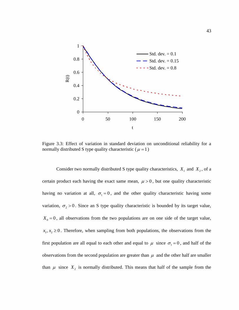
When fixing the mean and varying the standard deviation, the trend is different.

As it can be seen in figure (3.3) where 1 for all three cases, in the short run, a quality

characteristic with larger standard deviation results in a smaller unconditional reliability

compared to a quality characteristic with a smaller standard deviation. In the long run,

however, the opposite is true. That is, the quality characteristic with the larger standard

deviation results in a larger unconditional reliability compared to the quality

characteristic with the smaller standard deviation.

The behavior of the two cases corresponding to 0.1 and 0.15 in figure

(3.3) can be explained by the following example while the case of 0.8 has a different

interpretation as discussed below.

43

0

0.2

0.4

0.6

0.8

1

0 50 100 150 200

t

R(t

)

Std. dev. = 0.1

Std. dev. = 0.15

Std. dev. = 0.8

Figure 3.3: Effect of variation in standard deviation on unconditional reliability for a

normally distributed S type quality characteristic ( 1 )

Consider two normally distributed S type quality characteristics, 1X and 2X , of a

certain product each having the exact same mean, 0 , but one quality characteristic

having no variation at all, 1 0 , and the other quality characteristic having some

variation, 2 0 . Since an S type quality characteristic is bounded by its target value,

0 0X , all observations from the two populations are on one side of the target value,

1 2, 0x x . Therefore, when sampling from both populations, the observations from the

first population are all equal to each other and equal to since 1 0 , and half of the

observations from the second population are greater than and the other half are smaller

than since 2X is normally distributed. This means that half of the sample from the

44

second population is of worse quality (expected to fail earlier) than the sample from the

first population and the other half is of better quality (expected to last longer). Since one

of the definitions of the unconditional reliability R t is the proportion of the population

that survives until time t (Leemis, 2009), in the short run, 1 2R t R t when the less

reliable half of the sample from the second population tends to fail. As time passes, on

the other hand, 2 1R t R t when the sample from the first population tends to fail

while the better quality half of the second population tends to survive longer. This

example fully explains the behavior of the two cases corresponding to 0.1 and

0.15 seen in figure (3.3).

The case of 0.8 in figure (3.3) is unrealistic since such a large standard

deviation compared to the mean would imply that some of the quality characteristic

values are negative and this contradicts the fact that an S type quality characteristic is

bounded by zero. Thus, the normality assumption of the quality characteristic does not

hold anymore. This case is presented in figure (3.3) only to show how the same behavior

as the other two cases ( 0.1 and 0.15 ) is amplified by higher standard deviation

but for a different reason.

The effect of varying the standard deviation while keeping the mean constant

shown in figure (3.3) can also theoretically be seen in an N type quality characteristic if

the mean setting has a relatively high offset from the target compared to the standard

deviation. This situation, however, is not common in practice since it would be too

obvious for process controllers or inspectors that the process setting is grossly off. On the

other hand, it could be stated that, for an N type quality characteristic, if the mean setting

45

is exactly on target, it is always the case that the higher the standard deviation, the lower

the quality and reliability of the product.

3.2.2 Normally Distributed L Type Quality Characteristic

An L type quality characteristic is the case in which it is desired to have the value

of the quality characteristic to be as large as possible. Therefore, as the value of the

quality characteristic of a given product gets larger, the more reliable the product

becomes. This effect can be seen in figure (3.4) in which the conditional reliability

(equation (2.16)) increases as the value of the quality characteristic increases. Like all

reliability functions, the conditional reliability decreases with time for all cases.

0

0.2

0.4

0.6

0.8

1

0 50 100 150 200

t

R(t

|x)

x = 60

x = 50

x = 40

Figure 3.4: Effect of variation in x on conditional reliability for a normally distributed L

type quality characteristic

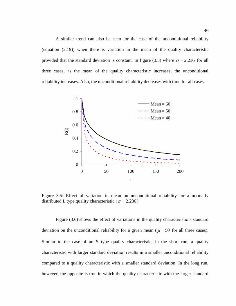
46

A similar trend can also be seen for the case of the unconditional reliability

(equation (2.19)) when there is variation in the mean of the quality characteristic

provided that the standard deviation is constant. In figure (3.5) where 2.236 for all

three cases, as the mean of the quality characteristic increases, the unconditional

reliability increases. Also, the unconditional reliability decreases with time for all cases.

0

0.2

0.4

0.6

0.8

1

0 50 100 150 200

t

R(t

)

Mean = 60

Mean = 50

Mean = 40

Figure 3.5: Effect of variation in mean on unconditional reliability for a normally

distributed L type quality characteristic ( 2.236 )

Figure (3.6) shows the effect of variations in the quality characteristic’s standard

deviation on the unconditional reliability for a given mean ( 50 for all three cases).

Similar to the case of an S type quality characteristic, in the short run, a quality

characteristic with larger standard deviation results in a smaller unconditional reliability

compared to a quality characteristic with a smaller standard deviation. In the long run,

however, the opposite is true in which the quality characteristic with the larger standard

47

deviation results in a larger unconditional reliability compared to the quality

characteristic with the smaller standard deviation. This behavior can be explained in a

similar manner as in the case of an S type quality characteristic since the inverse of an L

type quality characteristic is an S type quality characteristic. For an L type quality

characteristic, however, the target value is infinite and all observations of the quality

characteristic are less than the target value, x . Again, the case of 40 shown in

figure (3.6) is unrealistic since 50 and it is only provided for illustrative purposes.

0

0.2

0.4

0.6

0.8

1

0 50 100 150 200

t

R(t

)

Std. dev. = 2.236

Std. dev. = 10

Std. dev. = 40

Figure 3.6: Effect of variation in standard deviation on unconditional reliability for a

normally distributed L type quality characteristic ( 50 )

It is to be noted that the values of LR t in figures (3.5) and (3.6) are calculated

numerically using equation (2.19). Therefore, in order to examine the adequacy of the

48

approximate expression of LR t given by equation (2.23), the same cases shown in

figures (3.5) and (3.6) were repeated using the approximate LR t and the maximum

percentage errors were calculated. As it can be seen from table (3.1), the maximum

percentage error gets smaller as the ratio increases. Since it is quite common for the

mean of an L type quality characteristic to be much larger than its standard deviation, it

can be concluded that the approximate expression of LR t , i.e. equation (2.23), is fairly

adequate for most real life applications.

Maximum % error between

numerical and approximate LR t

1.25 89

5 10

17.9 1.18

22.4 0.6

26.8 0.27

Table 3.1: Effect of on the accuracy of the approximate unconditional reliability

function of an L type quality characteristic

3.2.3 Beta Distributed Quality Characteristics

Since the beta distribution is much more flexible than the normal distribution, the

quality characteristic that follows a beta distribution can have a variety of shapes. That is,

as was mentioned in section (2.2.4), depending on the values of the two shape parameters

and , the distribution of the quality characteristic could be strictly increasing or

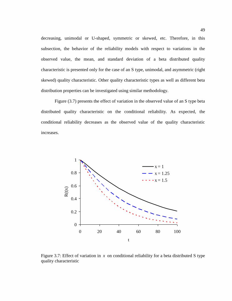
49

decreasing, unimodal or U-shaped, symmetric or skewed, etc. Therefore, in this

subsection, the behavior of the reliability models with respect to variations in the

observed value, the mean, and standard deviation of a beta distributed quality

characteristic is presented only for the case of an S type, unimodal, and asymmetric (right

skewed) quality characteristic. Other quality characteristic types as well as different beta

distribution properties can be investigated using similar methodology.

Figure (3.7) presents the effect of variation in the observed value of an S type beta

distributed quality characteristic on the conditional reliability. As expected, the

conditional reliability decreases as the observed value of the quality characteristic

increases.

0

0.2

0.4

0.6

0.8

1

0 20 40 60 80 100

t

R(t

|x)

x = 1

x = 1.25

x = 1.5

Figure 3.7: Effect of variation in x on conditional reliability for a beta distributed S type

quality characteristic

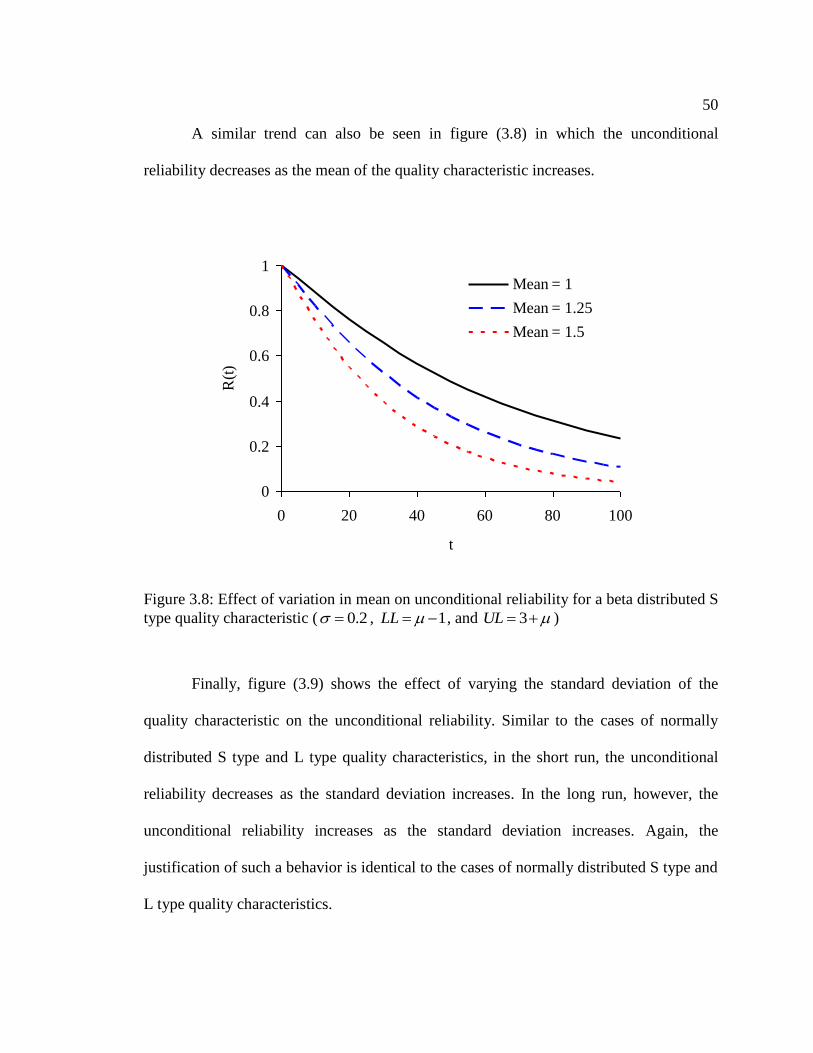
50

A similar trend can also be seen in figure (3.8) in which the unconditional

reliability decreases as the mean of the quality characteristic increases.

0

0.2

0.4

0.6

0.8

1

0 20 40 60 80 100

t

R(t

)

Mean = 1

Mean = 1.25

Mean = 1.5

Figure 3.8: Effect of variation in mean on unconditional reliability for a beta distributed S

type quality characteristic ( 0.2 , 1LL , and 3UL )

Finally, figure (3.9) shows the effect of varying the standard deviation of the

quality characteristic on the unconditional reliability. Similar to the cases of normally

distributed S type and L type quality characteristics, in the short run, the unconditional

reliability decreases as the standard deviation increases. In the long run, however, the

unconditional reliability increases as the standard deviation increases. Again, the

justification of such a behavior is identical to the cases of normally distributed S type and

L type quality characteristics.

51

0

0.2

0.4

0.6

0.8

1

0 20 40 60 80 100

t

R(t

)

Std. dev. = 0.2

Std. dev. = 0.5

Std. dev. = 0.7

Figure 3.9: Effect of variation in standard deviation on unconditional reliability for a beta

distributed S type quality characteristic ( 1 , 0LL , and 4UL )

3.3 Numerical Example

In this section, a comprehensive numerical example is presented in which the

procedure of applying the methods developed in this study in real life problems is shown.

The procedure begins with a set of raw data. Table (3.2) presents a set of time to failure

data of a normally distributed L type quality characteristic. The mean and standard

deviation of the quality characteristic x in the sample data set are 32.7 and 4.5,

respectively. There are 14 pairs of data points which are assumed to be uncensored.

52

sample x t

1 25.42 24.08

2 27.43 26.11

3 28.03 29.99

4 28.69 27.97

5 32.20 26.32

6 32.57 34.26

7 32.78 40.59

8 32.87 60.79

9 33.06 58.55

10 33.63 53.20

11 34.66 64.81

12 34.94 74.15

13 37.81 72.92

14 43.16 83.06

Table 3.2: Sample data set of failure times of an L type quality characteristic

Using MLE, the reliability model scaling parameters are found using the

likelihood function given by equation (2.39) as follows:

1

1

2 2

1

2 2

1

2 2

, ; , , , ; , ,

24.08 exp 24.0825.42 25.42

* 26.11 exp 26.1127.43 27.43

* * 83.06 exp43.16 43.16

n

i i

i

c c

c c

c

L t x a b c f t x a b c

b ba c a

b ba c a

b ba c a

83.06c

(3.1)

53

The likelihood function in equation (3.1) is then maximized using a nonlinear

optimization program. The reliability model scaling parameters were found to be 0a ,

0.011b , and 2.9c . Next, the unconditional reliability LR t is calculated. Using

both the numerical and approximate solutions, i.e. equations (2.19) and (2.23),

respectively, the results of LR t calculations are shown in table (3.3) and figure (3.10).

Numerical LR t Approximate LR t % Error

1.0000 1.0000 0.00

0.9988 0.9988 0.00

0.9914 0.9911 0.02

0.9723 0.9716 0.07

0.9374 0.9358 0.17

0.8842 0.8813 0.33

0.8121 0.8075 0.57

0.7235 0.7168 0.92

0.6228 0.6140 1.40

0.5163 0.5058 2.04

0.4112 0.3996 2.83

0.3139 0.3020 3.78

0.2292 0.2181 4.84

0.1599 0.1504 5.96

0.1065 0.0990 7.02

0.0676 0.0623 7.87

0.0410 0.0375 8.34

0.0237 0.0217 8.18

0.0130 0.0121 7.12

0.0068 0.0065 4.77

0.0034 0.0034 0.67

Table 3.10: Calculated values of the numerical and approximate LR t solutions of the

numerical example including the % error between the two solutions

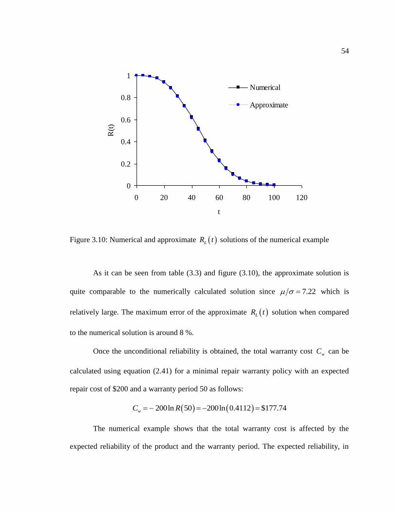
54

0

0.2

0.4

0.6

0.8

1

0 20 40 60 80 100 120

t

R(t

)

Numerical

Approximate

Figure 3.10: Numerical and approximate LR t solutions of the numerical example

As it can be seen from table (3.3) and figure (3.10), the approximate solution is

quite comparable to the numerically calculated solution since 7.22 which is

relatively large. The maximum error of the approximate LR t solution when compared

to the numerical solution is around 8 %.

Once the unconditional reliability is obtained, the total warranty cost wC can be

calculated using equation (2.41) for a minimal repair warranty policy with an expected

repair cost of $200 and a warranty period 50 as follows:

200ln 50 200ln 0.4112 $177.74wC R

The numerical example shows that the total warranty cost is affected by the

expected reliability of the product and the warranty period. The expected reliability, in

55

turn, is affected by the mean setting and variance of the quality characteristic. Therefore,

based on the mean setting and variance of the quality characteristic, using the reliability

models developed in this study, an estimate of the total warranty cost could be found for

a given warranty period.

56

Chapter 4

Summary, Conclusions, and Future Research

4.1 Summary and Conclusions

From the literature review, it was concluded that even though Taguchi’s quadratic

loss function was a clear improvement over the goal post mentality, it still was very

simplistic in nature and extremely difficult to implement with accuracy in reality.

Therefore, there have been many attempts to find alternatives to Taguchi’s loss function.

One of these attempts has been the work by Deleveaux (1997) who used

reliability models to connect the effects of mean setting and variance of a quality

characteristic on the reliability of a product. Then, using warranty models, the reliability

of the product was presented in monetary value thereby making a connection between the

quality of a product (in terms of conformance to targets and variance) and external failure

costs. The only problem was that a closed-form solution of the reliability function could

not be developed by Deleveaux (1997). Blue (2001), however, using the same approach

as Deleveaux (1997) but with a different reliability model, was able to find a closed-form

solution to the reliability model of a normally distributed N type quality characteristic.

Because of that, the models by Blue (2001) had the most potential for further study.

The objectives of this study were to extend the work by Blue (2001) to include

normally distributed S type and L type quality characteristics as well as beta distributed

quality characteristics. Expressions for the conditional and unconditional reliability

57

functions as well as the hazard and probability density functions were developed for all

cases. However, due to the mathematical complexity of the unconditional reliability,

hazard, and probability density functions expressions for the cases of normally distributed

L type quality characteristic as well as beta distributed quality characteristics, closed-

form expressions could not be found for these cases. Instead, an approximate solution

was found for the case of normally distributed L type quality characteristic, which was

compared to a solution found numerically, while the beta distributed quality characteristic

cases were all solved numerically.

This study also demonstrated the methodology of how to estimate the scaling

parameters of the reliability models using maximum likelihood estimation (MLE).

Moreover, a detailed description of the procedure and computer algorithm used for

numerical integration of some of the reliability models was presented.

The reliability models developed in this study were then validated by examining

the effects of variations in the observed value of the quality characteristic on the

conditional reliability and the effects of variations in mean and standard deviation of the

quality characteristic on the unconditional reliability.

Finally, an illustrative numerical example was presented that outlined the

procedure of implementing the reliability and warranty models developed in this study on

a practical problem.

58

4.2 Future Research

Since most products consist of a number of critical components, one direction for

future research would be to extend all reliability models considered in this study to

include more than one quality characteristic. That is, applying the current reliability

models to systems with series and/or parallel components that could be either

independent or dependent with each other. This way, a better estimate of external failure

costs of a product could be achieved.

Another extension of the current study would be to apply the reliability and

warranty models to real life problems. This would require collecting real data either from

the industry or by conducting life testing experiments. Collecting real data from industry

is especially challenging since there is either a lack of comprehensive and accurate data

or, due to confidentiality policies, these data cannot be released (Deleveaux, 1997). Thus,

life testing experiments could be the more viable option for collecting data and validating

this study’s models.

Other extensions include considering more sophisticated and realistic warranty

models as well as conducting return on investment analysis when, for instance, different

machines with varying quality and reliability are considered for purchase.

59

Bibliography

Barlow, R. and Hunter, L., “Optimum Preventive Maintenance Policies,” Operations

Research, 8, 1, pp. 90-100, 1960.

Blue, J., Reliability Functions Incorporating the Mean and the Variance, M.S Thesis,

Industrial and Manufacturing Engineering, Penn State University, 2001.

Casella, G. and Berger, R., Statistical Inference, 2nd

Edition, Duxbury Press, Pacific

Grove, CA, 2002.

Chandra, M. J., Statistical Quality Control, CRC Press, Boca Raton, FL, 2001

Deleveaux, V., Analytical Models for Justification of Investment in Continuous Quality

Improvement, PhD Dissertation, Industrial and Manufacturing Engineering, Penn

State University, 1997.

Elsayed, E., Reliability Engineering, Addison Wesley Longman, Inc., Reading, MA,

1996.

Lee, H., “The Investment Model in Preventive Maintenance in Multi-Level Production

Systems,” International Journal of Production Economics, 112, 2, pp. 816-828,

2008.

Leemis, L., Reliability: Probabilistic Models and Statistical Methods, 2nd

Edition,

Prentice Hall, Englewood Cliffs, New Jersey, 2009.

60

Leung, B., and Spiring, F., “The Inverted Beta Loss Function: Properties and

Applications,” IIE Transactions, 34, 12, pp. 1101-1109, 2002.

Li, M., “A general Model for Process-Setting with an Asymmetrical Linear Loss

Function,” International Journal of Advanced Manufacturing Technology, 26, 11-

12, pp. 1317-1322, 2005.

Maghsoodloo, S., Ozdemir, G., Jordan, V., and Huang, C., “Strengths and Limitations of

Taguchi’s Contributions to Quality, Manufacturing, and Process Engineering,”

Journal of Manufacturing Systems, 23, 2, pp. 73-126, 2004.

Nguyen, D. and Murthy, D., “A General Model for Estimating Warranty Costs for

Repairable Products,” IIE Transactions, 16, 4, pp. 379-386, 1984.

Nocerito, G., Justification of Investment in Training, M.S Thesis, Industrial Engineering

and Operations Research, Penn State University, 2002.

Sauer, T., Numerical Analysis, Pearson Addison Wesley, Boston, MA, 2006.

Schneider, H., Pruett, J., and Lagrange, C., “Uses of Process Capability Indices in the

Supplier Certification Process,” Quality Engineering, 8, 2, pp. 225-235, 1995.

Spiring, F., “The Reflected Normal Loss Function,” The Canadian Journal of Statistics,

21, 3, pp. 321-330, 1993.

Spiring, F. and Yeung, A., “A General Class of Loss Functions with Industrial

Applications,” Journal of Quality Technology, 30, 2, pp. 152-162, 1998.

Taguchi, G., Elsayed, E., and Hsiang, T., Quality Engineering in Production Systems,

McGraw-Hill, New York, 1989.

61

Taguchi, G., and Clausing, D., “Robust Quality,” Harvard Business Review, 68, 1, pp.

65-75, 1990.

Zhang, Y., An Alternative to Taguchi’s Loss Function Using Capability Index, M.Eng.

Scholarly Paper, Industrial and Manufacturing Engineering, Penn State

University, 2006.

62

Appendix A

MATLAB Codes Used for Numerical Integration

A.1 Normally Distributed L type Quality Characteristic

In this section, the MATLAB m-files used for the numerical integration of a

normally distributed L type quality characteristic are presented. Three m-files are needed

for this numerical integration. These m-files are param_normal, ltb_normal, and

adapquad. All the parameters needed for the numerical integration are specified in

param_normal. Then, ltb_normal, which utilizes adapquad, is called in MATLAB to get

the results. The three m-files are listed below.

A.1.1 param_normal.m

% The parameters of the unconditional reliability model for the

% normally distributed x are:

%the reliability model's parameters:

a = 0;

b = 0.011;

c = 2.9;

%mean and variance of the normally distributed x and the process target:

mean1 = 32.7;

var1 = 4.5^2;

%upper and lower limits of the integration (theoretically,

%-inf to +inf):

ll = 5;

ul = 60;

63

%integration accuracy (error tolerance):

tol0 = 0.0000005;

%warranty period:

w = 200;

%calculate the reliability every "inc" during the warranty period:

inc = 5;

A.1.2 ltb_normal.m

%Input: specify parameters in param_normal.m for the normally

% distributed x (x is L type)

%Output: the unconditional reliability at different t

param_normal

for t=0:inc:w

%here, s1 and s2 are different chunks of the expression that

%is being integrated and s is the whole expression put together.

clear s1 s2 s

s1 = ['exp(-(' num2str(a) '+' num2str(b) '*(1/x)^2)*' num2str(t) '^' num2str(c) ')'];

s2 = ['*1/(2*' num2str(pi) '*' num2str(var1) ')^0.5*exp(-(x-' num2str(mean1) ')^2/2/'

num2str(var1) ')'];

s = [s1 s2];

f = inline(s);

integral=adapquad(f,ll,ul,tol0)

end

A.1.3 adapquad.m

% Matlab code from Sauer (2006) pp. 271

% Input: a Matlab inline function f, interval [u0,v0],

% error tolerance tol0

% Output: the numerical integration of f

function integral=adapquad(f,u0,v0,tol0)

integral=0;

n=1;

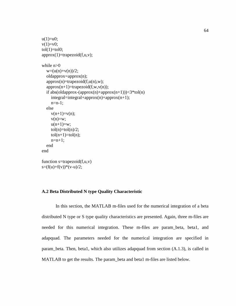
64

u(1)=u0;

v(1)=v0;

tol(1)=tol0;

approx(1)=trapezoid(f,u,v);

while n>0

w=(u(n)+v(n))/2;

oldapprox=approx(n);

approx(n)=trapezoid(f,u(n),w);

approx(n+1)=trapezoid(f,w,v(n));

if abs(oldapprox-(approx(n)+approx(n+1)))<3*tol(n)

integral=integral+approx(n)+approx(n+1);

n=n-1;

else

v(n+1)=v(n);

v(n)=w;

u(n+1)=w;

tol(n)=tol(n)/2;

tol(n+1)=tol(n);

n=n+1;

end

end

function s=trapezoid(f,u,v)

s=(f(u)+f(v))*(v-u)/2;

A.2 Beta Distributed N type Quality Characteristic

In this section, the MATLAB m-files used for the numerical integration of a beta

distributed N type or S type quality characteristics are presented. Again, three m-files are

needed for this numerical integration. These m-files are param_beta, beta1, and

adapquad. The parameters needed for the numerical integration are specified in

param_beta. Then, beta1, which also utilizes adapquad from section (A.1.3), is called in

MATLAB to get the results. The param_beta and beta1 m-files are listed below.

65

A.2.1 param_beta.m

% The parameters of the unconditional reliability model for the

% beta distributed x are:

%the reliability model's parameters:

a = 0;

b = 0.01;

c = 1.1;

%gamma and eta of the beta distributed x and the process target:

gamma1 = 18.5;

eta1 = 55.5;

x0 = 0;

%upper and lower limits of the integration:

ll = 0;

ul = 4;

%integration accuracy (error tolerance):

tol0 = 0.0000005;

%warranty period:

w = 200;

%calculate the reliability every "inc" during the warranty period:

inc = 5;

A.2.2 beta1.m

%Input: specify parameters in param_beta.m for the beta

% distributed x

%Output: the unconditional reliability at different t

param_beta

%calculate the beta function B(gamma,eta) appearing in the pdf of the beta

%distribution

B = beta(gamma1,eta1);

for t=0:inc:w

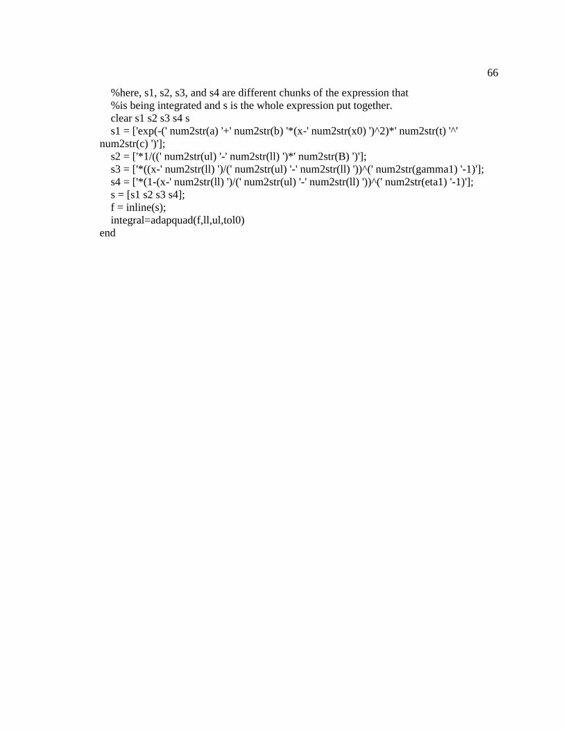
66

%here, s1, s2, s3, and s4 are different chunks of the expression that

%is being integrated and s is the whole expression put together.

clear s1 s2 s3 s4 s

s1 = ['exp(-(' num2str(a) '+' num2str(b) '*(x-' num2str(x0) ')^2)*' num2str(t) '^'

num2str(c) ')'];

s2 = ['*1/((' num2str(ul) '-' num2str(ll) ')*' num2str(B) ')'];

s3 = ['*((x-' num2str(ll) ')/(' num2str(ul) '-' num2str(ll) '))^(' num2str(gamma1) '-1)'];

s4 = ['*(1-(x-' num2str(ll) ')/(' num2str(ul) '-' num2str(ll) '))^(' num2str(eta1) '-1)'];

s = [s1 s2 s3 s4];

f = inline(s);

integral=adapquad(f,ll,ul,tol0)

end