An alternative model to the open-economy “new consensus” ∗∗∗∗

Ricardo Summa

Abstract

In this paper we present a heterodox open-economy macroeconomic model aiming to establish an alternative view to the "New Consensus" model and analyze the determinants of long-run inflation, the monetary policy transmission channels, the costs of such policy and some barriers to its implementation. The open-economy New Consensus model with inflation targeting is based on the following theoretical structure: (i) the potential output is determined according to the neoclassical theory of value and distribution; (ii) output depends on the real interest rate and the real exchange rate (iii) the Phillips curve is accelerationist (iv) the exchange rate determination depends on the uncovered interest rate parity in the short run and on the purchasing power parity in the long run; (v) a Taylor rule. The main results of this model are well known. There is no trade-off between inflation and productive capacity, since the later is independent of the effective output; and such policy can always be applied, because it is always possible to the Monetary Authority to fix the real interest rate in line with the natural rate of interest. The alternative model proposed follows the same simplified scheme of the New Consensus model, but altering significantly some theoretical assumptions. (i) First, the potential output or productive capacity of the economy follows the long-run expected effective demand. We use the Sraffian supermultiplier to model the demand led growth of productive capacity. (ii) the output growth rate depends on the real interest rate (through the effect on autonomous spending) and the real exchange rate (through the effect on exports), (iii) the Phillips curve is non accelerationist (partial inertia hypothesis) and depends on the role of nominal exchange rate, on the imported inflation and on the degree of distributive conflict, (iv) the nominal exchange rate depends on the interest rate differential and is subject to speculation, and (v) a Taylor rule. We analyze the alternative model in terms of analytic solution and computer simulations. The main results of this model is that the long-run inflation will depend on imported inflation, on the distributive conflict and on the inertia degree in the economy; demand shocks influences inflation only in the short run, so the main channel to control inflation by MA is by controlling the nominal exchange rate appreciation through the maintenance of an interest rate differential with the rest of the world. From the cost of policy standpoint, the results also differ from that proposed by the New Consensus. First, we show that the policy of inflation control is not neutral in terms of growth rate of productive capacity. This means that a higher inflation targeting or a lower imported inflation ultimately lead to a higher growth rate of productive capacity (so the external constraint can appear in the form of higher imported inflation); moreover, as the policy of inflation control depends largely on a process of nominal exchange rate appreciation, the consequence is that the real exchange rate will also appreciate and this will bring a deteriorating trend on the Balance of Trade and Current Account. Finally, the anti-inflationary policy is not neutral in terms of functional income distribution. We also show that there are limitations to applying such policy. International liquidity conditions and opposition of political groups to a process of real exchange rate appreciation are important sources of such limitations. In sum, there are limitations in implementing such policy, which depends on the external, political and institutional factors.

∗Professor Adunto at Instituto de Economia, Federal University of Rio de Janeiro. I would like to thank to Franklin Serrano, Carlos Pinkusfeld, Fabio Freitas, Nicholas Trebat, Miguel Bruno and Gilberto Libanio for very helpful comments and to IPEA/PNDP for financial support.

2

1. Introduction

The new consensus or the “three equation” model was fully analyzed by Carlin and

Soskice (2010), Romer (2000), Taylor (1997,2000) and now is becoming popular even

in the undergraduate textbooks (Mankiw, 2010). The New Consensus model with

inflation targeting is based on the following theoretical structure: (i) the effective output

depends on the real interest rate (stimulating investment spending), (ii) the existence of

an accelerationist Phillips curve and (iii) a Taylor rule, relating the Monetary Authority

response via nominal interest rate to deviations of inflation from its target and output

from its potential. The potential output is determined by the stocks of factors of

production – capital and labor - and their productivity, according to the neoclassical

theory of value and distribution;

In an open-economy context, the new consensus model postulates that the Real Interest

Rate Parity holds (Romer, 2006). It is implicit on this assumption that that the

Uncovered Interest Rate Parity holds in the short run and that the individuals operating

in the exchange rate market have Rational Expectations and believe that the Purchasing

Power Parity holds in the long run (Lavoie, 2000);

The main results of this model are well known. The long-run core inflation is related

with demand shocks and does not depend on the exchange rate (open-economy long run

neutrality); the inflation control mechanism involves the impact of the real interest rate

on aggregate demand, targeting a null output gap. There is no trade-off between

inflation and productive capacity, since the latter is independent of the effective output1;

and such policy can always be applied, because the Monetary Authority can always set

the real interest rate in line with the natural rate of interest.

There are, however, a considerable number of works that evaluate critically the new

consensus model in a closed-economy context. They show that by changing some of the

hypotheses of this model (such as the accelerationist Phillps Curve), the model

generates very different results in terms of output, inflation and productive capacity

(Setterfield (2004); Lavoie e Kriesler (2005); Aspromorgous (2007); Serrano (2007)).

1In fact, although not explicit, “new consensus” economists believe that there is a negative relationship between high inflation rates and productive capacity, in the sense that high inflation can create some inefficiencies, lowering the growth rates of potential output. Lavoie (2006) call this relationship “the hidden equation”.

3

In this paper we present a heterodox open-economy macroeconomic model that seeks to

establish an alternative view to the "New Consensus" model and analyze the

determinants of long-run inflation, the transmission channels for monetary policy, the

costs of such policy and its implementing limitations.

2. Alternative model to the open-economy “new consensus”

The alternative model presented here follows the same simplified scheme of the New

Consensus model, but alters significantly some theoretical assumptions. (i) First, the

potential output or productive capacity of the economy follows the long-run expected

effective demand. We use the Sraffian supermultiplier to model the demand led growth

of productive capacity. (ii) the output growth rate depends on the real interest rate

(through the effect on autonomous spending) and the real exchange rate (through the

effect on exports), (iii) the Phillips curve is non accelerationist (partial inertia

hypothesis) and depends on the role of nominal exchange rate, on the imported inflation

and on the degree of distributive conflict, (iv) the nominal exchange rate depends on the

interest rate differential and is subject to speculation, and (v) the Monetary Authority

seeks to achieve a pre-defined inflation target, through changes in nominal interest rate.

2.1 The Sraffian Supermultiplier and IS curve

The first assumption of the alternative model is that the potential output or productive

capacity of the economy (��� follows the long-run expected effective demand. We use

the Sraffian supermultiplier (Serrano (1996)) to model the demand-led growth of

productive capacity.

Following the Surplus Approach (Garegnani, 1990), the potential output will be

constrained by the most scarce factor, given the technical coefficients (Serrano, 2008).

Assuming that in a capitalist economy in general we have no labor scarcity, the productive

capacity of this economy is constrained by the amount of capital. Thus, the economy’s

productive capacity will be the same as the capital stock potential output, which depends on the

size of the capital stock and the technical coefficient. This means that the potential output

can be reached even with labor unemployment.

We use the standard notation. In Equation (1)Y is the current level of effective demand

and output. Equations (2) and (3) show the components of the aggregate demand. In (2)

we suppose a simple Kaleckian consumption function, where aggregate consumption

(C) depends on the Wage Bill (wage share (w� times disposable national income) and

4

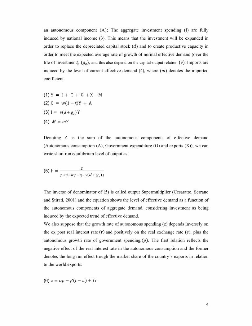
an autonomous component �A�; The aggregate investment spending (I) are fully

induced by national income (3). This means that the investment will be expanded in

order to replace the depreciated capital stock (�) and to create productive capacity in

order to meet the expected average rate of growth of normal effective demand (over the

life of investment), (��), and this also depend on the capital-output relation (�). Imports are

induced by the level of current effective demand (4), where () denotes the imported

coefficient.

(1) � � � � � ��� � ��� � � � � (2) �� � ���� � ��� � ��� (3) � � )( egdv + � (4) � � �

Denoting Z as the sum of the autonomous components of effective demand

(Autonomous consumption (A), Government expenditure (G) and exports (X)), we can

write short run equilibrium level of output as:

(5) � � ������������� )( egdv + �

The inverse of denominator of (5) is called output Supermultiplier (Cesaratto, Serrano

and Stirati, 2001) and the equation shows the level of effective demand as a function of

the autonomous components of aggregate demand, considering investment as being

induced by the expected trend of effective demand.

We also suppose that the growth rate of autonomous spending (z) depends inversely on

the ex post real interest rate�� ��and positively on the real exchange rate (!), plus the

autonomous growth rate of government spending,�"�. The first relation reflects the

negative effect of the real interest rate in the autonomous consumption and the former

denotes the long run effect trough the market share of the country’s exports in relation

to the world exports:

(6) # � $" � %�& � '� � (!

5

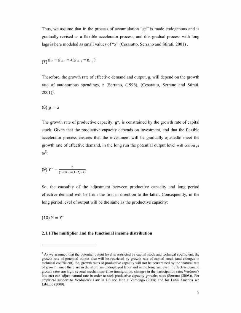
Thus, we assume that in the process of accumulation “ge” is made endogenous and is

gradually revised as a flexible accelerator process, and this gradual process with long

lags is here modeled as small values of “x” (Cesaratto, Serrano and Stirati, 2001) .

(7))(1 jtjetetet ggxgg

−−−−+=

Therefore, the growth rate of effective demand and output, g, will depend on the growth

rate of autonomous spendings, z (Serrano, (1996), (Cesaratto, Serrano and Stirati,

2001)).

(8) � � #

The growth rate of productive capacity, g*, is constrained by the growth rate of capital

stock. Given that the productive capacity depends on investment, and that the flexible

accelerator process ensures that the investment will be gradually ajustedto meet the

growth rate of effective demand, in the long run the potential output level will converge

to2:

(9) �� � �������������)�

So, the causality of the adjustment between productive capacity and long period

effective demand will be from the first in direction to the latter. Consequently, in the

long period level of output will be the same as the productive capacity:

(10) � � �

2.1.1The multiplier and the functional income distribution

2 As we assumed that the potential output level is restricted by capital stock and technical coefficient, the growth rate of potential output also will be restricted by growth rate of capital stock (and changes in technical coefficient). So, growth rates of productive capacity will not be constrained by the ‘natural rate of growth’ since there are in the short run unemployed labor and in the long run, even if effective demand grotwh rates are high, several mechanisms (like immigration, changes in the participation rate, Verdoon’s law etc) can adjust natural rate in order to seek productive capacity growths rates (Serrano (2008)). For empirical support to Verdoorn’s Law in US see Jeon e Vernengo (2008) and for Latin America see Libânio (2009).

6

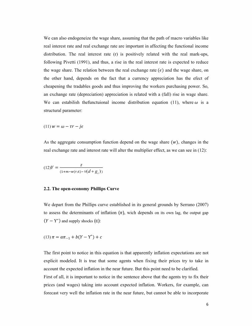
We can also endogeneize the wage share, assuming that the path of macro variables like

real interest rate and real exchange rate are important in affecting the functional income

distribution. The real interest rate (r) is positively related with the real mark-ups,

following Pivetti (1991), and thus, a rise in the real interest rate is expected to reduce

the wage share. The relation between the real exchange rate��!� and the wage share, on

the other hand, depends on the fact that a currency appreciation has the efect of

cheapening the tradables goods and thus improving the workers purchasing power. So,

an exchange rate (depreciation) appreciation is related with a (fall) rise in wage share.

We can estabilish thefunctuional income distribution equation (11), where�* is a

structural parameter:

(11)�+ � *� ,- � .!

As the aggregate consumption function depend on the wage share �+�, changes in the

real exchange rate and interest rate will alter the multiplier effect, as we can see in (12):

(12)� � ��������/01�� )( egdv + �

2.2. The open-economy Phillips Curve

We depart from the Phillips curve established in its general grounds by Serrano (2007)

to assess the determinants of inflation ('), wich depends on its own lag, the output gap

�� � ���and supply shocks (c):

(13)�' � 2'�� � 3�� � �� � 4

The first point to notice in this equation is that apparently inflation expectations are not

explicit modeled. It is true that some agents when fixing their prices try to take in

account the expected inflation in the near future. But this point need to be clarified.

First of all, it is important to notice in the sentence above that the agents try to fix their

prices (and wages) taking into account expected inflation. Workers, for example, can

forecast very well the inflation rate in the near future, but cannot be able to incorporate

7

the whole forecasted inflation in their wage contracts, depending on their bargaining

power (Rowthorn, 1977).

Moreover, inflation expectations are revised accordingly to inflation levels in the recent

past, and thus, it is difficult to support the view that inflation expectations are

exogenous. In this way, recent past inflation is a good proxy to expected inflation.3 So,

part of the lagged inflation in the Phillips Curve (13) can be explaind as backward-

looking expectations.

The other part of the lagged inflation can be explained by structural and institutional

factors. Industrial capitalist economies are organized into productive chains, so a change

in the price of raw materials, for example, translates into higher costs for intermediate

and final goods, and this price transmission process takes some time. In this way, part of

the inflation inertia could be explained by itrinsic characteristics of an input-output

economy. Furthermore, there are institutional factors like contracts estabilishing

automatic price adjustment, based in recent performance of some price index.

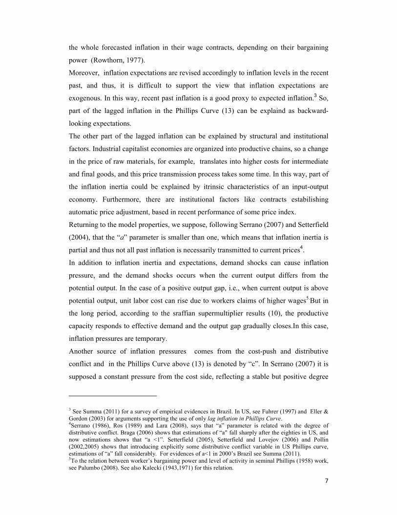
Returning to the model properties, we suppose, following Serrano (2007) and Setterfield

(2004), that the “a” parameter is smaller than one, which means that inflation inertia is

partial and thus not all past inflation is necessarily transmitted to current prices4.

In addition to inflation inertia and expectations, demand shocks can cause inflation

pressure, and the demand shocks occurs when the current output differs from the

potential output. In the case of a positive output gap, i.e., when current output is above

potential output, unit labor cost can rise due to workers claims of higher wages5.But in

the long period, according to the sraffian supermultiplier results (10), the productive

capacity responds to effective demand and the output gap gradually closes.In this case,

inflation pressures are temporary.

Another source of inflation pressures comes from the cost-push and distributive

conflict and in the Phillips Curve above (13) is denoted by “c”. In Serrano (2007) it is

supposed a constant pressure from the cost side, reflecting a stable but positive degree

3 See Summa (2011) for a survey of empirical evidences in Brazil. In US, see Fuhrer (1997) and Eller & Gordon (2003) for arguments supporting the use of only lag inflation in Phillips Curve. 4Serrano (1986), Ros (1989) and Lara (2008), says that “a” parameter is related with the degree of distributive conflict. Braga (2006) shows that estimations of “a" fall sharply after the eighties in US, and now estimations shows that “a <1”. Setterfield (2005), Setterfield and Lovejov (2006) and Pollin (2002,2005) shows that introducing explicitly some distributive conflict variable in US Phillips curve, estimations of “a” fall considerably. For evidences of a<1 in 2000’s Brazil see Summa (2011). 5To the relation between worker’s bargaining power and level of activity in seminal Phillips (1958) work, see Palumbo (2008). See also Kalecki (1943,1971) for this relation.

8

of distributive conflict. Serrano’s (2007) model results supposing partial inertia (a < 1),

output strong hysteresis (sraffian supermultiplier and�� � �) and constant degree of

distributive conflict is that economic policy trade-off will be between the general price

level and productive capacity6.

In the present model, we mantain the partial inertia and strong output hysteresis

hypothesis, but we alter the last one of a constant cost-push pressure. In an open-

economy context, we suppose that the cost-push inflation will depend on imported

inflation and the distributive conflict7.

Regarding imported inflation, it depends on the inflation of tradable goods but also on

nominal exchange rate changes. Despite the fact that we call this variable “imported”

inflation, it is not related only to inflation of imported – consumption, intermediate and

capital – goods, but also to tradable exportable goods, since a country exporters can

equalize the goods price in domestic and external markets.

The distributive conflict is explicit introduced in the model following Pivetti (1991),

Lima & Setterfield (2010) and Serrano (2010), supposing that changes in nominal

interest rate (5&) can affect inflation both from the financial cost channel (indebted

enterprises)and form oportunity cost of capitalchannel (as the nominal mark-up depends

on the long run nominal interest rate).8

So in our model we have the following Phillips curve:

(14) ' � 2'�� � 3�� � �� � 5& � 6�57 � '��, com 2 8 �

Where 57 refers to nominal exchange rate change ; '� �tradable goods inflation

(measured in international currency); and�6�is a parameter which reflects the tradable

goods share in domestic price index.9.

In attempting to close our model, we need only to discuss the nominal interest rate

setting mechanism and exchange rate determination.

6SeeSerrano (2007). 7See Serrano and Summa (2011) and Braga and Bastos (2011) for this discussion and empirical support in Brazilian case. 8 For empirical evidences and theoretical discussion about this relation, see Lima e Setterfield (2010). For a survey on brazilian Price Puzzle empirical evidences see Summa (2011). 9 Note that the tradable goods share refers not only to final goods but also to tradable inputs goods used to produce non-tradable goods.

9

2.3. Nominal exchange rate determination

In order to analyze the nominal exchange rate determination we need to look at the

economy’s balance of payments. The balance of payments is obtained by summing the

balance of current account������with financial account. We can also separate the

financial account between the short run��9:;��and long run capital flows (9<;�.

(15)=> � �� � 9<; � 9:;

In a flexible exchange rate regime, we have a zero balance of payments, so the current

account balance must equal the financial account balance:

(16)9:; � ��� � 9<;

Supposing that long run capital flows are exogenous determined, we must analyze the

determinants of short run capital flows and current account balance. In our model, the

short run capital flows depends on the interest rate differential between the domestic

interest rate �?� and international rate �?@� (plus the sovereign spread (A� and expected

exchange rate change�B��C � B�). The parameter F is an autonomous term of short run

capital flowsand D is the sensivity of short run capital flows to interest rate differentials.

The current account balance depends on the real exchange rate.

(17)9:; � 9 � D�? � �?@ � A � �B��C � B)))

It is important to notice that the domestic interest rate does not necessarily adjust to the

international rate (plus sovereign spread end Exchange rate change expectations). So the

Monetary Authority can institutionally fix the domestic interest rate, and thus stimulate

capital inflows or outflows.10.

10See Pivetti (1991) and Serrano e Summa (2012b) for the exogenous interest rate approach. For interest rate exogeneity even in open economies, see Lavoie (2000,2001,2002-2003) and Pivetti (2001).

10

Supposing also that the international rate (?@� and the sovereign spread11(A��are

exogenous variables, we just need to discuss the exchange rate expectations to solve the

nominal exchange rate determination problem.

We assume that expected nominal exchange rate, (B��C ), is at least in part endogenous

and dependent on the evolution of the nominal exchange rate occurred in the near past.

This is because the foreign currency can be seen as an asset, subject to speculation

(Frenkel & Taylor, 2006). After a continuous process of nominal exchange appreciation,

further appreciation could be expected in the future. Dealers speculating in the exchange

rate market will thus avoid buying foreign currency expecting that its price will be

lower in the near future. This will lead to another round of currency appreciation,

because foreign currency sellers will have to lower its price and buyers will only buy it

if the price is lower. As a consequence, a process of exchange rate appreciation can lead

to expectations of appreciation (the same is valid with processes of exchange rate

devaluation) (Serrano and Summa, 2012a).

Exogenous shocks can influence expectations, like good or bad news about the future

path of some external variables that affect currency dealers’ opinions about the

exchange rate that will prevail in the future, reversing or aggravating the process

described above.

In the model, the best way to formalize the process described above is that the exchange

rate expectations are in part adaptative, and subject to exogenous shocks (E� related to

news about relevant variables that influences currency dealers’ expectations:

(18) 7��� � 7� � F�7�� � 7�� � G,com 3 H �.

If we assume, attempting to simplify the model, that h=1 and�E � I, expectations about

exchange rate will depend only on the exchange rate prevailing one period ago:

(19) 7��� � 7��

Replacing equation(17) in (16) we have:

11 The assumption of exogenous sovereign spread is quite strong, but in section 4.6 we discuss some results when relaxing this hypothesis.

11

(20) ��� � 9<; � 9 � D�? � �?@ � A � �B��C � B���

Equation (20) determinesthe balance of payments equilibrium. Denoting 9Jas the sum of

the exogenous flows and the current account balance (9J � 9 � �� � 9<;��, rearranging

(20) and substituting nominal exchange rate expectations (19) we have:

(21) 7 � 7�� � �& � ?@ � A� � KLM

Nominal exchange rate will thus depend on the past exchange rate, interest rate

differential (plus sovereign spread), exogenous capital flows and current account

balance. And the change in nominal exchange rate �7 � 7��� depends on the interest

rate differential. This means that a positive and constant interest rate difeerential will

lead to a process of nominal exchange rate appreciation through time.12

This results from the exchange rate expectation effect through current exchange rate. A

positive interest rate differential, in the context where expectations are elastic, can lead

to process of exchange rate appreciation, and this will bring expectations of other

currency appreciation, valuating exchange rate again, and so on. The same unstable

process can occur if the monetary authority fix permanently the domestic interest rate

bellow international rate (plus sovereign spread). In pratice, monetary authorities are

forced to manipulate interest rate differentials together with interventions in currency

market, buying and selling foreign reserves. As pointed out in Serrano & Summa

(2012a), there is no such thing as a free floating regime.

This process can be influenced by International liquidity conditions (for example, an

improvement in international liquidity conditions can raise autonomous capital

flows�9J� and lower sovereign spread �A)).

12Notice that this result differs from uncovered interest parity models. In Brazilian Central Bank model

(Bogdanski et alli (2000)), for example, a positive interest rate differential leads to an once and for all nominal exchange rate appreciation through time, while in our model a process of nominal exchange rate appreciation follows from a positive interest rate differential.

12

3. Model closure and analytical solution

To close our model we need to establish how the interest rate is determined. We

suppose, as in the new consensus model, that the monetary authority fixes the nominal

interest rate in order to achieve inflation target �πN). The Monetary Authority raises the

nominal interest rate when inflation is above target, and lowers when it is below:

(21) ? � ?�� � O�P � PN�

In order to obtain the analytical solution, we depart from the Phillips curve (Equation

14). The long run inflation will depend on the permanent pressures on inflation.

Demand shocks, as we discuss, are temporary as the productive capacity adjusts to the

current output level. In the long run, this source of pressure disappears. Cost-push

shocks such as changes in nominal interest rates (5? ) are also temporary, supposing that

there is a nominal interest rate (? � ?N� that is capable of achieving inflation target. So,

in the long run we do not expect changes in the nominal interest rate.

Consequently, in the long run, inflation will depend on international inflation, changes

in nominal exchange rate, the share of tradable in domestic general price index and on

the inflation inertia degree:

(22) ' � Q�5��RS���T

We have the following system to solve:

(6) # � $ � %�& � '� � (! (20) 57 � ��& � &� � U� � KL

M (21) & � &�� � V�' � 'W� (22) ' � Q�5��RS�

��T

From Equation (22) we can deduce that, given international inflation, the share of

tradable goods in domestic general price index and inflation inertia degree, there is a

change in nominal exchange rate that can bring long run inflation to the target.

13

To achieve this exchange rate change, the monetary authority must fix domestic interest

rate above international rate. We will denote the domestic interest rate necessary to

change nominal exchange rate and thus to bring long run inflation to the target as (&W�. Replacing equation (22) in (20) and as P � PN X ? � ?N, we have:

(23) 'W � Q�RS�YZ[\�[S�]^�_L` a�

��T

Thus, the domestic interest rate necessary to change nominal exchange rate and thus to

bring long run inflation to the target (&W� will be:

(24) &W � '� � �&� � U� � KLM � R\���T�

Q

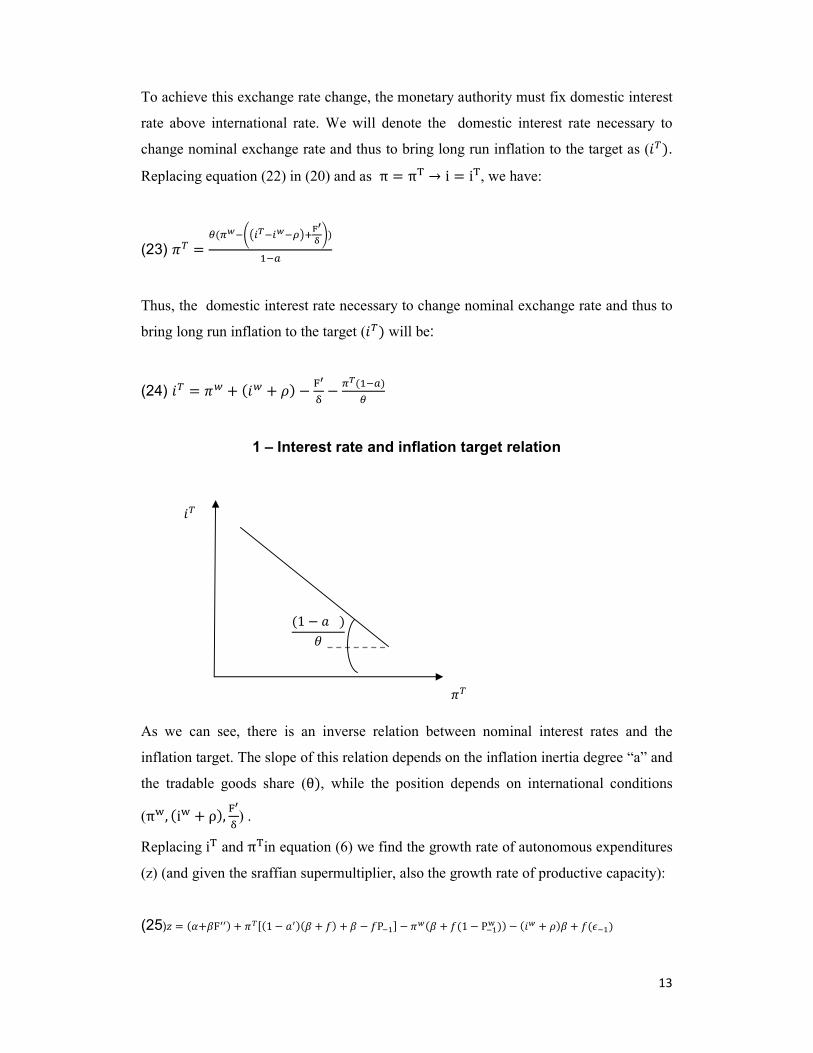
1 – Interest rate and inflation target relation

As we can see, there is an inverse relation between nominal interest rates and the

inflation target. The slope of this relation depends on the inflation inertia degree “a” and

the tradable goods share (b�, while the position depends on international conditions

(P@0 �?@ � A�0 KLM ) .

Replacing ?N and PNin equation (6) we find the growth rate of autonomous expenditures

(z) (and given the sraffian supermultiplier, also the growth rate of productive capacity):

(25)# � �$�%9JJ� � 'Wc�� � 2J��% � (� � % � (>��d � '��% � (�� � >��@ �� � �&� � U�% � (�!���

&W

'W

�� � 2 �6

14

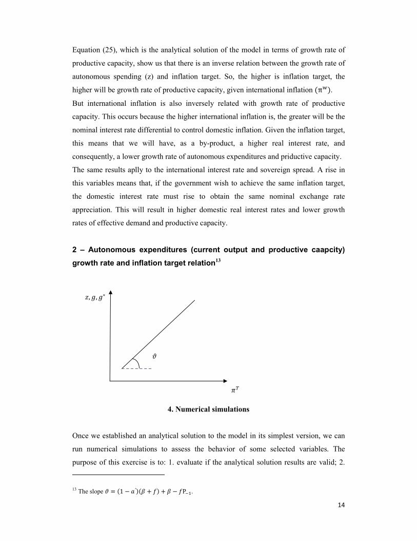
Equation (25), which is the analytical solution of the model in terms of growth rate of

productive capacity, show us that there is an inverse relation between the growth rate of

autonomous spending (z) and inflation target. So, the higher is inflation target, the

higher will be growth rate of productive capacity, given international inflation �P@�. But international inflation is also inversely related with growth rate of productive

capacity. This occurs because the higher international inflation is, the greater will be the

nominal interest rate differential to control domestic inflation. Given the inflation target,

this means that we will have, as a by-product, a higher real interest rate, and

consequently, a lower growth rate of autonomous expenditures and priductive capacity.

The same results aplly to the international interest rate and sovereign spread. A rise in

this variables means that, if the government wish to achieve the same inflation target,

the domestic interest rate must rise to obtain the same nominal exchange rate

appreciation. This will result in higher domestic real interest rates and lower growth

rates of effective demand and productive capacity.

2 – Autonomous expenditures (current output and productive caapcity)

growth rate and inflation target relation13

4. Numerical simulations

Once we established an analytical solution to the model in its simplest version, we can

run numerical simulations to assess the behavior of some selected variables. The

purpose of this exercise is to: 1. evaluate if the analytical solution results are valid; 2.

13 The slope e � �� � 2′��% � (� � % � (>��.

#0 �0 ��

'W

e

15

analyze the path of some selected variables when some simplifying assumptions are

dropped off; 3. evaluate the dynamic path in direction (or not) to the equilibrium

position.

We will assess the path results of: 1. growth rates of productive capacity when we have

different (a) inflation target; (b) internatinal inflation rate; (c) international interest rate

and sovereign spread; 2. The Current Trade Balance; (c) Income functional distribution.

We can also check the hypothesis that, if the monetary authority controls the nominal

interest rate, it can controls inflation rate in direction to the target when the core

inflation is cost-push and related with imported inflation. And finally, it will be

analyzed the dynamic path of real interest rate, real exchange rate and output gap related

to different inflation targets.

In the numerical simulation exercise, the extreme hypothesis of h =1 in the adaptative

exchange rate expectation (18) is abandoned and the exchange rate expectations now

depends on an average weight of past exchange rate.

The initial condition, parameters and exogenous variables supposed are: a) inflation

starts at 5%; b) First exchange rate expectations is 4,0 and the parameter h is 0,76; c)

International interest rate is 5% and sovereign spread is 2%; d) initial domestic nominal

interest rate is 9%; d) Output and productive capacity initial levels are in equilibrium

and are equal to 400; e) Exogenous component of growth rate of autonomous

expenditures, $is 5%; f) The monetary authority’s rule parameter V is 0,7; g) a high

value of δ0 denoting that short run capital flows are highly sensitive to interest rate

differentials; h) structural component of functional income distribution equation is

* � I0f1.

All the simulations start with the same initial conditions, and the parameters and

exogenous variables are changed in period 10.

4.1 Alternative Inflation Target

In the first exercise, we change the monetary authority inflation target in order to

analyze alternative paths of productive capacity growth rate, inflation rate, real interest

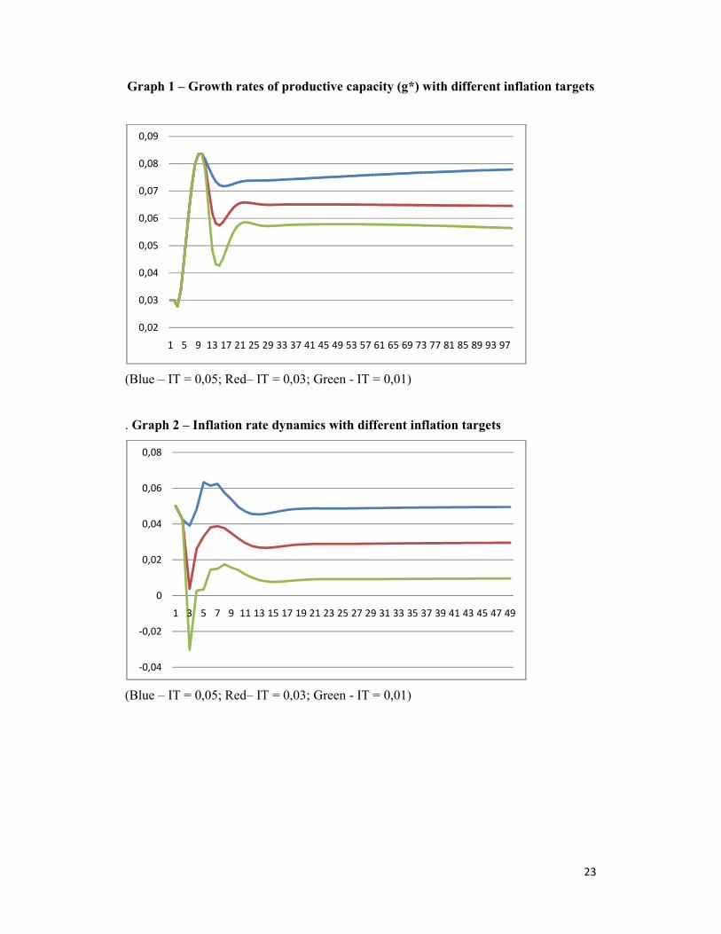
rate, real exchange rate and output gap. Graph 1 shows the growth rate of capacity paths

to different inflation targets (1%, 3% and 5%). As it was expected, lower inflation

targets will generate, as a by-product, lower growth rates of productive capacity.

Inflation dynamics with different inflation targets are showed in graph 2. It is interesting

16

to note that Monetary Authority can achieve inflation rate target in the three cases. It

means that, even in an economy where the core inflation is cost-pushed and related with

imported inflation, it is possible to MA to control inflation rate using nominal interest as

the only policy instrument.

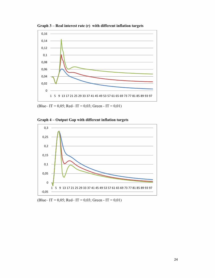
Graph 3 shows the dynamics paths of the real interest rate. Notice that this graph is

closely related to graph 1 discussed above. It shows that when the inflation target is

lower, it is necessary to fix a higher nominal interest rate, resulting in a higher ex post

real interest rate (higher nominal rate plus lower inflation rate), and this will lead to

lower growth rates of productive capacity (as showed in graph 1).

Output gap behavior is showed in graph 4. We can see that output gap endogenously

tends to close in the three cases, although it will take longer time to converge when

inflation target (and so growth rates of productive capacity) is higher.We can see in

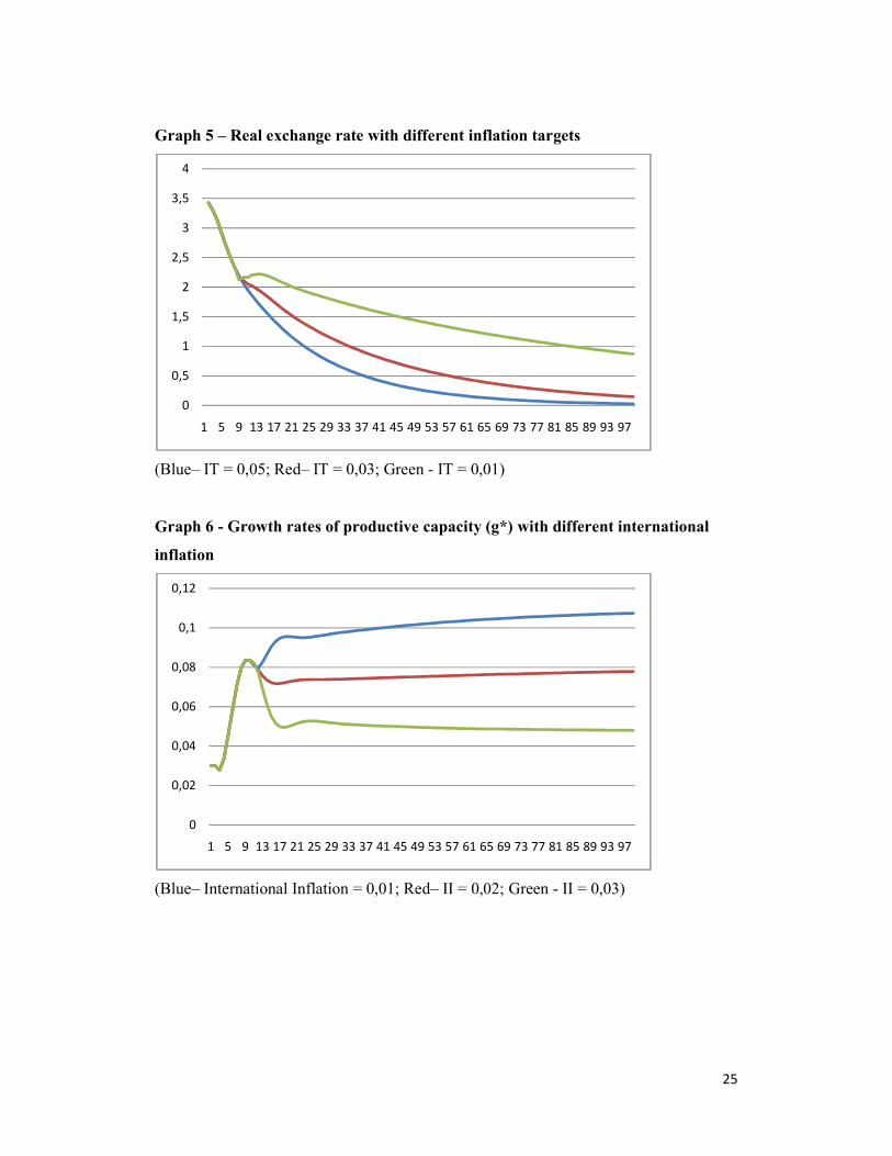
graph 5 the path of real exchange rate. The result shows that, given that this domestic

economy face an international inflation and has an inflation target, the nominal

exchange rate will appreciate more than ‘inflation differential’, resulting in real

exchange rate appreciation too. Note that this occurs to the three different inflation

targets. The higher is the inflation target, the higher will be “inflation differential”, and

this will lead to a quicker process of real exchange rate appreciation.

The last point to notice is that all the results were obtained with the monetary policy

rule parameter V =0,7. Even with these parameter, inflation converges to the target as

the MA fixes domestic nominal interest rate.This result could be seen as puzzling to one

that believes in the ‘new consensus model’relations, since in this model the V parameter

must be greater than one, that is, the nominal interest rate must raise more than the

difference between inflation and inflation target, in order to guarantee a real interest rate

change in the right direction. The point is that in the ‘new consensus model’, MA must

change the real interest rate in order to affect output gap, and so to control demand-

pulled inflation pressures.

In our model, the transmission mechanism is from the nominal interest rate - through

nominal interest rate differential with nominal international interest rate plus sovereign

spread – to the nominal exchange rate, which adaptative expectations can lead to a

process of nominal exchange rate appreciation (or depreciation) and so to affect

inflation through time. So, it is easy to understand that a change in the nominal interest

rate, even if it coincides at first with a change in the real interest rate in the opposite

direction, can control inflation.

17

4.2 International inflation

Now, we run another exercise changing international inflation and observing the results

in relation to different international inflation. The growth rates paths of productive

capacity related to these different international inflation rates are illustrated in graph 6.

As discussed in model’s analytical solution, if the economy faces a lower international

inflation, given the inflation target, the growth rate of productive capacity will be higher

than if it faces a higher international inflation. This happens because MA will need a

lower effort in appreciating nominal exchange rate, and it requires a lower interest rate

differential, resulting in lower levels of real interest rate and, consequently, higher rates

of growth of productive capacity.

This result calls attention to another way of interpreting external constraint in demand-

led growth models. This means that demand-led growth of productive capacity can be

restricted by economic policy objectives (in this case, inflation target) depending on the

external conditions (in this case, international inflation).

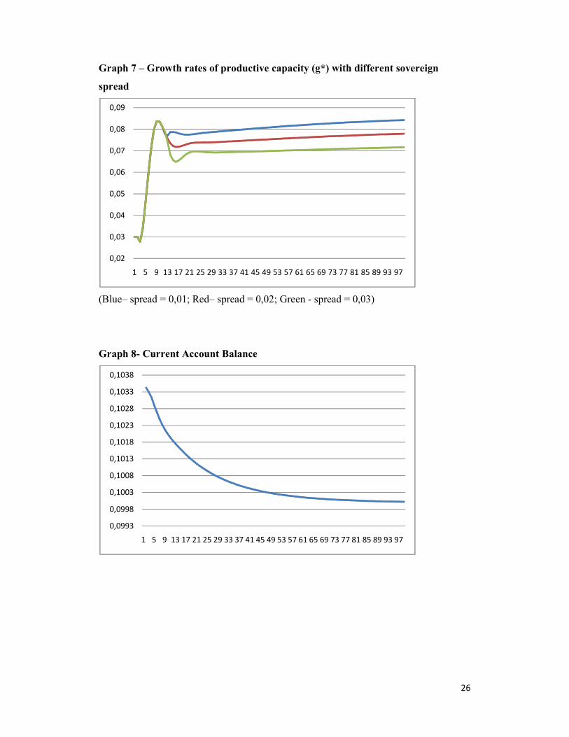
4.3 International interest rate and sovereign spread

The same results are obtained when we alter international interest rate (or sovereign

spread), indicating another sources of demand-led growth constraint due to external

conditions when a country seeks some economic policy target.In this case, a rise in

international interest rate due to, for example, autonomous changes in US monetary

policy, or a rise in country’s sovereign spread as consequence of a worsen in

international liquidity conditions, will result in lower growth rates of productive

capacity (see graph 7).This occurs because, in order to maintain the same interest rate

differential, it is necessary that the MA must raise domestic interest rate, with

consequences to growth rates of effective demand and productive capacity.

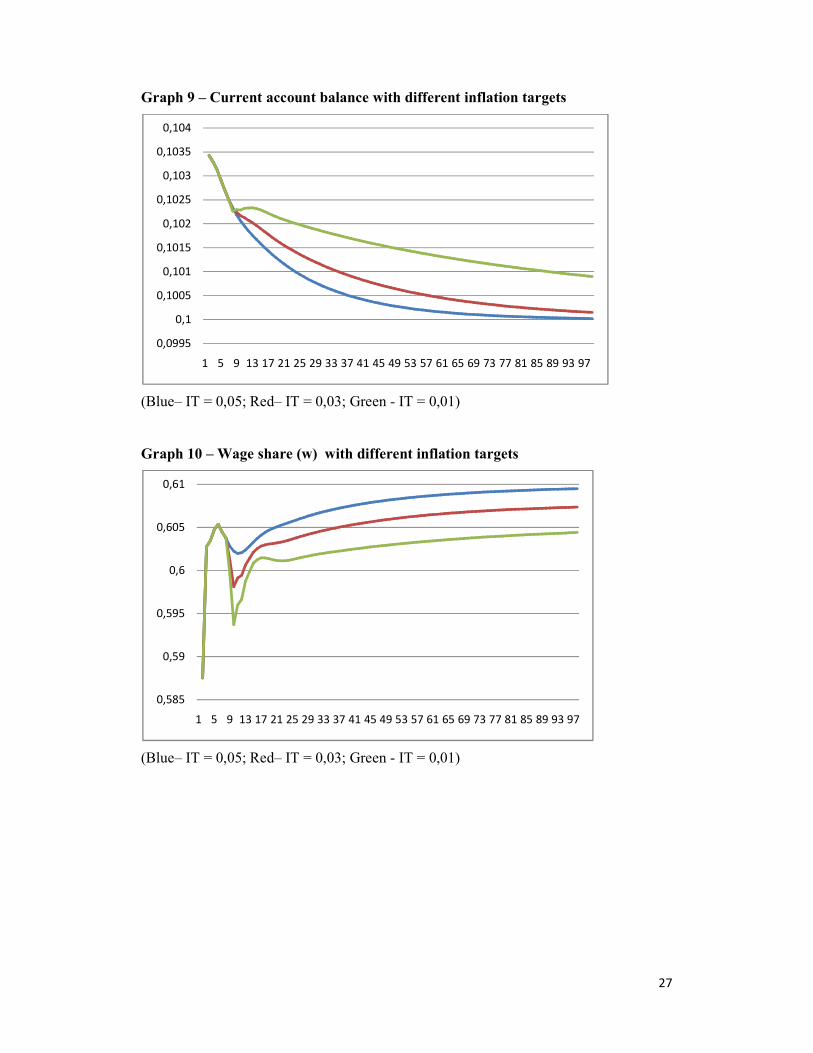
4.4 Current account Balance

Current account balance depends on the real exchange rate. As we saw in graph 6

above, one of the results of this model is that real exchange rate will appreciate

continuously, given an inflation target and an inflation control policy based on nominal

18

exchange rate appreciation. So, consequently, trade account balance will reduce

continuously (graph 8). This result occurs to different inflation targets, although the

higher is the inflation target, the quicker will be the current account balance reduction .

(graph 9), as the real Exchange rate appreciation path will be faster in this case.

4.5 Functional Income Distribution

In graph 10 we can see the functional income distribution results to different inflation

targets. The conclusion is that the higher is inflation target, the higher will be the wage

share on income. This occurs by two reasons: 1. The real interest rate will be lower

when inflation target is higher, and this will lead to lower mark-ups in the long run; 2.

Real exchange rate appreciate quicker when inflation target is higher, and this lowers

the price level and thus improve real wages.

4.6 Some limits to inflation control in this framework

Until now we discussed external constraints to demand-led growth of productive

capacity, that is, given some international inflation (or international interest rate levels)

the growth rates of productive capacity will be lower, as a by-product of achieving a

pre-established inflation target.

But we also need to considerer the impossibility of a MA in attaining inflation target,

depending on the external conditions of a country or international conditions in general.

As discussed before, given an international inflation, the only way of a country to seek

an inflation target when inflation is cost-pushed is by appreciating constantly the

nominal exchange rate. This will lead to a process of continuous appreciation of real

exchange rate, diminishing trade account balance until the country faces a deficit. This

country needs to run a financial account surplus in order to clear BP. Suppose that part

of this financial account surplus consist in external indebtedness. Depending on

previously accumulated foreign reserves and on the size and terms of the external debt,

the country can face rising sovereign spreads to finance current account deficits or even

an international credit rationing (Serrano e Summa, 2012a).

If it happens, MA loses control in attracting short run capital flows. So, the inflation

target policy will last until MA still has foreign reserves and can control nominal

19

exchange rate.When the stock of foreign reserves is depleted, the inflation target must

be abandoned.

This process can be generated endogenously as described above or even exogenously, if

for some reason international credit markets worsen suddenly and international credit is

rationed worldwide. Generally, MA is forced to abandon IT due to an unstable process

of exchange rate depreciation.14

Other limits to inflation control can arise from political disputes over different groups.

Some organized political groups which depend on competitive exchange rates ( to

export their goods and services, for example) can oppose to a process of real exchange

rate appreciation, and if they are successful in stopping the appreciation process, the

inflation will not converge to its target.

It is important to note that this impossibility of attaining IT can happen even if MA has

‘full credibility’. It is not a question of credibility, but of ‘structural’ external or political

conditions. In sum, there are limitations in implementing such policy, which depends on

the external, political and institutional factors.

5. Conclusion

In this paper we presented ademand-led growth of productive capacity model which is

restricted by economic policy objetives (in this case, inflation target) and this constraint

depends mainly on the evolution of country’s external accounts, international credit

market conditions and international inflation.

The long-run costs of pursuing such policy are evaluated in terms of rate of growth of

productive capacity, the trend in the Balance of Payments and the income distribution to

different inflation targets. First, we show that the policy of inflation control is not

neutral in terms of growth rate of productive capacity, since controlling inflation

through the nominal exchange rate appreciation needs a positive interest rate

differential, and, as a result, it impacts on the real interest rate and output/capacity

growth rates. Hence, a higher inflation targeting or a lower imported inflation ultimately

leads to a higher growth rate of productive capacity; moreover, as the policy of inflation

control depends largely on a process of nominal exchange rate appreciation, the

14In Brazil 2000’s we observed the validity of Barbosa’s Law (Serrano & Summa 2011), that is, inflation target was only achieved when nominal exchange rate appreciate. In the years of external crises like 2001-2003, inflation rate was higher than inflation target (Barbosa Filho, 2008).

20

consequence is that the real exchange rate will also appreciate and this will bring a

deteriorating trend on the Balance of Trade and Current Account. Finally, the anti-

inflationary policy is not neutral in terms of functional income distribution. Since the

distribution depends on the real interest rate and real exchange rate, a lower inflation

target will lead to higher real interest rates and, consequently, the income distribution

will change, reducing the wage share.

Thus, we also argue that the international inflation has a role in influencing the long run

growth rate of productive capacity. This occurs because when the economy experiences

a raise in the international inflation, it impacts on the long run domestic inflation, and

the Monetary Authority reacts raising the interest rate differential to appreciate the

nominal exchange rate faster, in order to reach the inflation target. A higher real interest

rate is a by-product of such policy, and has consequences on lowering the growth rate of

current output and productive capacity. So, we show that the external constraint can

appear in the form of higher imported inflation.

We discussed also that there can be limitations to operating such policies and this

depends on a country political and external conditions or international conditions in

general.

Finally, it is important to notice that we are not proposing here a rule of thumb or a

stable and well-defined set of choices between economic policy objetives (inflation

target) and outcomes (growth rate of productive capacity, external account, functional

income distribution). What we want to call atention is that in an open-economy, in

which growth rate of productive capacity is demand-led and MA follows some explicit

economic policy objectives (like inflation target), there will be real costs in achieving

policy targets, and these costs will depend on external conditions.

References

ASPROMOURGOS, T. “Interest as an Artefact of Self-Validating Central Bank Beliefs”, Metroeconomica, 2007.

BARBOSA-FILHO, N.H. “Inflation Targeting in Brazil: 1999 – 2006; International Review of Applied Economics”, Vol. 22, No.2, pp. 187 – 200, 2008.

BOGDANSKY, J. ; TOMBINI, A. ; WERLANG, S. (2000) “Implementing Inflation Targeting in Brazil”. Banco Central do Brasil Working Paper, n. 1, July.

BRAGA, J. Raiz unitária, inércia e histerese: o debate sobre as mudanças da NAIRU na economia americana nos anos 1990. Unpublished Phd Thesis, IE-UFRJ, 2006.

CARLIN, W. & SOSKICE Teaching Intermediate Macroeconomics using the 3-Equation Model In: Fontana, Giuseppe, and Mark Setterfield, (2010). Macroeconomic Theory and Macroeconomic Pedagogy Palgrave MacMillan

21

Publishers Limited Houndmills, Basingstoke, Hampshire, RG21 6XS, England, 2010

CESARATTO, S.; SERRANO, F. ; STIRATI, A. “Technical Change, Effective Demand and Employment”, Review of Political Economy, vol. 15, n. 1, pp. 33 – 52, 2003.

ELLER, J . W. ; GORDON, R. J. Nesting the New Keynesian Phillips curve within the mainstream model of U.S. inflation dynamics, Konferenzbeitrag, CEPR Conference "'The Phillips Curve revisited" in Berlin, 5.-7. June 2003.

FRENKEL, R. & TAYLOR, L. “Real Exchange Rate, Monetary Policy and Employment” DESA Working Paper No. 19, United Nations, February 2006

FUHRER, J., “The (Un)Importance of Forward-Looking Behavior in Price Specifications” Journal of Money Credit, and Banking, Vol, 29, No. 3, 1997.

GAREGNANI, P. "Sraffa: Classical versus Marginalist Analysis", in Essays on Piero Sraffa: Critical Perspectives on the Revival of Classical Theory (Ed. by K. Bharadwaj and B. Schefold), Unwin-Hyman, 1990.

JEON, Y.; VERNENGO, M. Puzzles, Paradoxes and Regularities: Cyclical and Structural Productivity in the US (1950-2005), Review of Radical Political

Economics Summer 2008 vol. 40 no. 3 237-243, 2008. KALECKI, M.. "Political Aspects of Full Unemployment", Political Quarterly, V. 14

(Oct.-Dec.): 322-331, 1943. KALECKI, M. Class Struggle and the Distribution of National Income. Michal Kalecki.

Kyklos, vol. 24, issue 1, pages 1-9, 1971. LARA, F. Um estudo sobre moeda, juros e distribuição. Unpublished Phd Thesis, IE-

UFRJ, 2008. LAVOIE, M. “A Post Keynesian view of parity theorems”, Jornal of Post Keynesian

Economics , fall, 2000 LAVOIE, M. "The reflux mechanism and the open economy" in Rochon, L. &

Vernengo, M. "Credit, Interest Rates and Open Economy: Essays on Horizontalism", Edward Elgar, 2001

LAVOIE, M. “Interest Parity, risk premia, and Post Keynesian analysis”, Journal of Post Keynesian Economics , Winter, 2002-2003

LAVOIE, M. A post-Keynesian amendment to the New consensus on monetary policy, Metroeconomica, vol. 57, no. 2, pp. 165-192 , May 2006.

LAVOIE M.; KRIESLER P. “The New View On Monetary Policy: The New Consensus And Its Post-Keynesian Critique”, University of Ottawa, Feb. 2005

LIBÂNIO, G. Aggregate Demand and the Endogeneity of the Natural Rate of Growth: evidence from Latin American economies. Cambridge Journal of Economics, 33, 2009.

LIMA, G ; SETTERFIELD, M. Pricing behavior and the cost-push channel of monetary policy. Review of Political Economy, 22, 1, 19-40, 2010.

MANKIW, N. Macroeconomics. 7 ed. , Worth Publishers: NY, 2010 PALUMBO, A., Demand and supply forces vs institutions in the interpretations of the

Phillips curve, mimeo, Dipartamento di Economia, Roma Tre, 2008b. PIVETTI, M., Distribution, Inflation and Policy Analysis, Review of Political

Economy, Volume 19, Number 2, 243–247, April 2007, 1991. PIVETTI, M. "Monetary endogeneity and non-neutrality in a sraffian perspective" in in

Rochon, L. & Vernengo, M. Credit, Interest Rates and Open Economy: Essays on Horizontalism, Edward Elgar, 2001

PHILLIPS, A. W. ‘The relation between unemployment and the rate of change of money wage rates in the United Kingdom, 1861–1957’, Economica, 25, pp. 283–99,

22

1958. POLLIN, R. “Wage Bargaining and the US Phillips Curve: was Greenspan right about

traumatized workers in the 90s?” mimeo, Political Economy Research Institute, University of Massachusetts Amherst, 2002.

POLLIN, R. Contours of descent, Verso, New updated edition, 2005. ROMER, D. Keynesian macroeconomics without the LM curve, Journal of Economic

Perspectives, 14 (2), 149-169, 2000. ROMER, D. Short-Run Fluctuations, in:[http://elsa.berkeley.edu/~dromer], Jan. 2006 ROS, J. (1989). On inertia, social conflict, and the structuralist analysis of inflation.

WIDER, Working Paper 128, 1989. ROWTHORN, B. Conflict, inflation and money, Cambridge Journal of Economics,

Vol. 1, Issue 3, pp. 215-239, 1977 SETTERFIELD. M. Central banking, stability and macroeconomic outcomes: a

comparison of new consensus and post-Keynesian monetary macroeconomics In Lavoie, M.;Secareccia, M. (eds)Central Banking in the modern world: Alternative perspectives, Edward Elgar, Cheltenham, pp.35-56, 2004.

SETTERFIELD, M. “Worker Insecurity and U.S. Macroeconomic Performance During the 1990s” Review of Radical Political Economics, 2005.

SETTERFIELD, M. & LOVEJOY, T. Aspirations, bargaining power, and macroeconomic performance. JPKE, v. 29, n. 1, p. 117-148, 2006.

SERRANO, F. Inflação inercial e desindexação neutra. Anais da ANPEC, 1986. SERRANO, F. Review of Pivetti's essay on money and distribution. Contributions to

Political Economy, 1993. SERRANO, F. The Sraffian Supermultiplier, Unpublished Phd Thesis, Cambridge,

1996. SERRANO, F. Histéresis, dinâmica inflacionaria y el supermultiplicador sraffiano”.

Seminarios Sraffianos, UNLU-Grupo Luján. Colección Teoría Económica, Edicionones Cooperativas, 2007.

SERRANO, F. Acumulação de capital, poupança e crescimento IE-UFRJ, 2008, mimeo SERRANO, F. O conflito distributivo e a teoria da inflação inercial, Revista de

Economia Contemporanea, 2010. SERRANO, F. ; SUMMA, R.”Macroeconomic Policy, Growth and Income Distribution

in the Brazilian Economy in the 2000s”, Center for Economic and Policy Research. 2011.

SERRANO, F, SUMMA, R. Mundell-Fleming without the LM curve: the exogenous interest rate in an open economy, 16th ESHET Conference, St Petersburg. 2012a

SERRANO, F, SUMMA, R. “Uma sugestão para simplificar a teoria da taxa de juros exógena”. Anais do V Encontro da AKB, São Paulo. 2012b

SUMMA, R. “Uma avaliação critica das estimativas da curva de Phillips no Brasil.” Revista Pesquisa & Debate, São Paulo, volume 22, n. 2 (40). 2011.

TAYLOR, J. B. A Core of Practical Macroeconomics. American Economic Review, 87 (2), pp. 233 –235, May 1997.

TAYLOR, J. B. Teaching modern macroeconomics at the principles level, American Economic Review, 90 (2), pp. 90–4, 2000

23

Graph 1 – Growth rates of productive capacity (g*) with different inflation targets

(Blue – IT = 0,05; Red– IT = 0,03; Green - IT = 0,01)

. Graph 2 – Inflation rate dynamics with different inflation targets

(Blue – IT = 0,05; Red– IT = 0,03; Green - IT = 0,01)

0,02

0,03

0,04

0,05

0,06

0,07

0,08

0,09

1 5 9 13 17 21 25 29 33 37 41 45 49 53 57 61 65 69 73 77 81 85 89 93 97

-0,04

-0,02

0

0,02

0,04

0,06

0,08

1 3 5 7 9 11 13 15 17 19 21 23 25 27 29 31 33 35 37 39 41 43 45 47 49

24

Graph 3 – Real interest rate (r) with different inflation targets

(Blue– IT = 0,05; Red– IT = 0,03; Green - IT = 0,01)

Graph 4 – Output Gap with different inflation targets

(Blue– IT = 0,05; Red– IT = 0,03; Green - IT = 0,01)

0

0,02

0,04

0,06

0,08

0,1

0,12

0,14

0,16

1 5 9 13 17 21 25 29 33 37 41 45 49 53 57 61 65 69 73 77 81 85 89 93 97

-0,05

0

0,05

0,1

0,15

0,2

0,25

0,3

1 5 9 13 17 21 25 29 33 37 41 45 49 53 57 61 65 69 73 77 81 85 89 93 97

25

Graph 5 – Real exchange rate with different inflation targets

(Blue– IT = 0,05; Red– IT = 0,03; Green - IT = 0,01)

Graph 6 - Growth rates of productive capacity (g*) with different international

inflation

(Blue– International Inflation = 0,01; Red– II = 0,02; Green - II = 0,03)

0

0,5

1

1,5

2

2,5

3

3,5

4

1 5 9 13 17 21 25 29 33 37 41 45 49 53 57 61 65 69 73 77 81 85 89 93 97

0

0,02

0,04

0,06

0,08

0,1

0,12

1 5 9 13 17 21 25 29 33 37 41 45 49 53 57 61 65 69 73 77 81 85 89 93 97

26

Graph 7 – Growth rates of productive capacity (g*) with different sovereign

spread

(Blue– spread = 0,01; Red– spread = 0,02; Green - spread = 0,03)

Graph 8- Current Account Balance

0,02

0,03

0,04

0,05

0,06

0,07

0,08

0,09

1 5 9 13 17 21 25 29 33 37 41 45 49 53 57 61 65 69 73 77 81 85 89 93 97

0,0993

0,0998

0,1003

0,1008

0,1013

0,1018

0,1023

0,1028

0,1033

0,1038

1 5 9 13 17 21 25 29 33 37 41 45 49 53 57 61 65 69 73 77 81 85 89 93 97

27

Graph 9 – Current account balance with different inflation targets

(Blue– IT = 0,05; Red– IT = 0,03; Green - IT = 0,01)

Graph 10 – Wage share (w) with different inflation targets

(Blue– IT = 0,05; Red– IT = 0,03; Green - IT = 0,01)

0,0995

0,1

0,1005

0,101

0,1015

0,102

0,1025

0,103

0,1035

0,104

1 5 9 13 17 21 25 29 33 37 41 45 49 53 57 61 65 69 73 77 81 85 89 93 97

0,585

0,59

0,595

0,6

0,605

0,61

1 5 9 13 17 21 25 29 33 37 41 45 49 53 57 61 65 69 73 77 81 85 89 93 97