An Algorithm for Parallel Reconstruction of Jointly...

An Algorithm for Parallel Reconstruction of Jointly Sparse Tensors with

Applications to Hyperspectral Imaging∗

Qun Li

Microsoft Corporation

11025 NE 8th St., Bellevue, WA 98004

[email protected]

Edgar A. Bernal

United Technologies Research Center

411 Silver Ln., East Hartford, CT 06118

[email protected]

Abstract

A wide range of Compressive Sensing (CS) frameworks

have been proposed to address the task of color and hyper-

spectral image sampling and reconstruction. Methods for

reconstruction of jointly sparse vectors that leverage joint

sparsity constraints such as the Multiple Measurement Vec-

tor (MMV) approach have been shown to outperform Sin-

gle Measurement Vector (SMV) frameworks which don’t ex-

ploit such constraints. Recent work has shown that exploit-

ing joint sparsity while simultaneously preserving the high-

dimensional structure of the data results in further perfor-

mance improvements. In this paper, we introduce a par-

allelizable extension of a previously proposed serial ten-

sorial MMV approach which, like its predecessor, exploits

joint sparsity constraints multiple data dimensions simulta-

neously, but that, in contrast, is parallelizable in nature. We

demonstrate empirically that the proposed method provides

better reconstruction fidelity of hyperspectral imagery given

a fixed number of measurements, and that it is also more

computationally efficient than the current state of the art.

1. Introduction

The acquisition and storage of hyperspectral imagery

impose stringent hardware constraints which result in in-

creased cost and complexity of hyperspectral imagers. Hy-

perspectral imaging is the process of using specialized sen-

sors to collect image information across the electromagnetic

spectrum, often beyond the visible electromagnetic wave-

length range. A hyperspectral image can be represented as

a three-dimensional data cube where the first and second di-

mensions correspond to spatial data and the third dimension

corresponds to the spectral bands. Objects have their own

respective fingerprints known as spectral signatures; conse-

quently, there is a wide range of applications, e.g., remote

∗*This work was done while the authors were with PARC, A Xerox

Company

sensing, astronomy, mineralogy, agriculture, healthcare and

surveillance, that rely on decomposing a two-dimensional

image of a scene into its spectral bands in order to enable

object identification within the scene. The main disadvan-

tages of hyperspectral imaging are related to the intrinsic

high dimensionality of the data, which imposes storage,

computational, and sensitivity constraints. These factors

drive up the complexity and cost of traditional hyperspec-

tral imagers. Fortunately, there is significant redundancy in

hyperspectral images along both the spatial and the spectral

dimensions which can be exploited by judicious sampling

and reconstruction techniques, which in turn gives rise to

sensing equipment with reduced complexity and cost.

Compressive Sensing (CS) techniques have been pro-

posed which exploit redundancies in hyperspectral data in

order to improve the efficiency of the sampling and recon-

struction processes. CS techniques aim at reconstructing

sparse signals from a small number of linear measurements,

relative to the original signal dimensionality. CS is of-

ten posed as an optimization problem whose objective con-

sists in finding the solution of an underdetermined system

of equations under a set of sparsity constraints. A vector

x ∈ RN is called s-sparse if it has at most s non-zero en-

tries. In mathematical terms, the linear sampling process of

x results in a set of samples y ∈ Rm obtained by comput-

ing y = Ax. In this expression, A ∈ Rm×N , where m < N,

denotes the sampling matrix. The reconstruction process

attempts to recover x by finding a z ∈ RN that satisfies

z = argminz

‖z‖0 s.t. y = Az. (1)

These sampling and recovery processes constitute what

is traditionally termed the Single Measurement Vector

(SMV) framework. The ℓ0 minimization problem in Eq.1

is nonpolynomial-deterministic- (NP-) hard, and thus, com-

putationally intractable, so it is often approximated by op-

timizing its ℓ1 equivalent or by implementing greedy algo-

rithms.

When the signal to be reconstructed consists of a set of

vectors with common support, simultaneous sampling of

1 24

the vectors can lead to improved reconstruction. This is

the premise of the Multiple Measurement Vector (MMV)

approach [5]. Speficially, assume the signal to be recon-

structed consists of a set of q vectors x j ∈ RN with com-

mon support, that is, X = [x1|x2| . . . |xq] ∈ RN×q. Simulta-

neous sampling results in a set of q vectorial measurements

that can be represented in the form of a matrix Y ∈ Rm×q,

where m < N, obtained by computing Y = AX, where Y =[y1|y2| . . . |yq]. The optimization task in the MMV recovery

problem is often formulated as the following optimization

task:

Z = argminZ

‖Z‖2,0 s.t. Y = AZ, (2)

where ‖Z‖2,0 denotes the ℓ0 norm of the vector whose ele-

ments are ℓ2 norms of the rows of matrix Z [5].

1.1. Related Work

Approximations to the NP-hard problem from Eq. 2 have

been formulated. For example, convex-relaxation-based

[5, 6, 17, 16] and approximation [15] alternatives have been

proposed. The optimization-based approach from [15] ad-

dresses two problems simultaneously, namely providing an

approximate solution to Eq. 2 and applying the MMV re-

covery framework to the task of color image reconstruction.

This task, along with that of hyperspectral image sampling

and reconstruction (HSI), had previously been formulated

as a group-sparse recovery problem [14, 11]. The direct ex-

tension of [15] to HSI is trivial. Alternative solutions to Eq.

2 have also been proposed which enforce stricter constraints

on the MMV problem. Specifically, the work in [10, 4] im-

poses a low-rank constraint on the measurement matrix in

addition to the traditional joint sparsity constraints.

Traditional CS theory is well-suited for sampling and

reconstruction of one-dimensional signals, and naıve ex-

tensions of the CS framework to multidimensional prob-

lems typically rely on vectorial representations of the data,

which result in increased computational and memory re-

quirements. Additionally, methodologies that vectorize

high-dimensional data fail to preserve the inherent tenso-

rial nature of the data, which results in failure to exploit

correlations across the different dimensionalities. Exam-

ples of high-dimensional data that are not appropriately rep-

resented by vectors, and thus not adequately recovered by

vectorial methods, include color and hyperspectral images,

as well as video streams. Extensions of the CS theory to

multi-dimensional data with applications in HSI have re-

cently been addressed [2, 9, 7]. Most existing tensorial CS

approaches, however, still fail to leverage joint sparsity con-

straints.

To our knowledge, until the method in [3] was intro-

duced, no existing algorithm was capable of exploiting joint

sparsity across different signal elements, while at the same

time preserving the dimensionality of the data. In this pa-

per, we introduce a parallelizable variant of the algorithm

from [3] that surpasses it both in terms of reconstruction

performance and computational efficiency.

1.2. Contributions

We propose a parallelizable version of the approach pro-

posed in [3] which is, to our knowledge, the state-of-the-art

with regards to MMV recovery of a multidimensional signal

with jointly sparse components. The method in [3] is tenso-

rial in nature and, as such, achieves better performance than

competing methods because it is able to preserve the multi-

dimensional nature of the data being reconstructed. One of

its limitations lies in its sequential multi-stage implemen-

tation, given that it requires one reconstruction stage for

each of the tensorial modes. This modus operandi results in

decreased fidelity since the reconstruction error from early

stages propagates into subsequent stages. In contrast, the

algorithm proposed in this paper decouples the reconstruc-

tion stages for the multiple tensor modes, which results in

improved reconstruction quality and reduced computational

complexity: since the reconstruction stages are effectively

independent, they can be implemented in a parallel man-

ner. The proposed method, like its predecesor, is capable of

leveraging the tensorial nature of the data in the sampling

and reconstruction stages; its parallel nature, on the other

hand, enables it to provide improved reconstruction perfor-

mance and achieve increased computational efficiency.

2. Notation and Terminology

As per the convention used in [13][2], we use Italic char-

acters to represent scalar values (e.g.,a,B), bold-face char-

acters to represent vectors (e.g.,a,b), capital italic bold-

face characters to represent matrices (e.g.,A,B) and capi-

tal calligraphic characters to represent tensors (e.g.,A ,B).A tensor is a multidimensional array which may be used

to represent high-dimensional signals such as color and hy-

perspectral images and videos. Tensor X ∈ RN1×···×Nd has

order d (or is d-dimensional), and the dimensionality of

its ith mode (also denoted mode i) is Ni. In short, the or-

der or number of dimensions of a tensor corresponds to its

number of modes, and each mode has its own associated di-

mensionality. The remainder of this section provides a brief

overview of relevant multilinear algebra concepts.

Kronecker product The Kronecker product of matrices

A ∈ RI×J and B ∈ R

K×L, denoted by A ⊗ B, is a matrix

of size (I · K)× (J · L) which is computed as A ⊗ B =

a11B a12B · · · a1JB

a21B a22B · · · a2JB

......

. . ....

aI1B aI2B · · · aIJB

.

Mode-i fiber and mode-i unfolding The mode-i fibers of

tensor X = [xα1,...,αi,...,αd] ∈ R

N1×···×Ni×···×Nd are obtained

25

by fixing every index but αi. The mode-i unfolding of X ,

denoted X(i), is a matrix of size Ni × (N1 · . . . ·Ni−1 ·Ni+1 ·. . . ·Nd) whose columns are the mode-i fibers of X . We use

Ri(X ) to denote the space formed by the mode-i fibers of

X .

Mode-i product The mode-i product between tensor X =[xα1,...,αi,...,αd

] ∈ RN1×···×Ni×···×Nd and matrix U = [u j,αi

] ∈R

J×Ni is a tensor X ×i U ∈ RN1×···×Ni−1×J×Ni+1×···×Nd , and

is defined element-wise as

(X ×i U)α1,...,αi−1, j,αi+1,...,αd=

Ni

∑αi=1

xα1,...,αi,...,αdu j,αi

.

3. Tensorial compressive sensing of hyperspec-

tral images

In the context of this paper, a hyperspectral image is rep-

resented as a third-order tensorial data cube, the first two

tensorial modes of which correspond to the spatial dimen-

sions, and the third mode of which is associated with the

spectral dimension of the image. More specifically, the

sampled hyperspectral cube representing the image is a ten-

sor of order three X ∈ RNr×Nc×Nb , where Nr and Nc are the

number of rows and columns of the image, respectively, and

Nb is the number of spectral bands. As in most CS frame-

works, the proposed algorithm comprises a sampling and a

reconstruction stage. The sampling stage is identical to that

of [3], and involves the acquisition of a set of linear mea-

surements from the hyperspectral image of a scene of inter-

est. In the reconstruction stage, the hyperspectral represen-

tation of the scene is estimated by independently recovering

each tensorial mode from the measurements acquired in the

sampling stage. As in [3], we pose the image reconstruc-

tion problem in teh context of a tensorial MMV framework;

in contrast, the reconstruction stage of the proposed algo-

rithm is parallelizable, and differs from that in [3] which is

sequential in nature since it requires the reconstruction of

certain modes to be completed before the reconstruction of

other modes can take place.

3.1. Sampling stage

As in [3], the sampling of X involves the computation

of a set of mode-i products between X and sampling ma-

trices Ui, for i = 1,2, one for each spatial tensor mode. The

entries of the sampling matrices are randomly generated.

The outcome of the sampling stage is a tensor Y that can

be computed as

Y = X ×1 U1 ×2 U2, (3)

where U1 ∈ Rmr×Nr and U2 ∈ R

mc×Nc , where mr and mc are

the number of measurements along the mode 1 and mode 2

(e.g., columns and rows) respectively, and Y ∈ Rmr×mc×Nb .

It should be appreciated that the outcome of the sampling

stage is still a tensor of order 3, in contrast with vectorial

methods (see, e.g., [15]) where the dimensions of the mea-

surement matrix are effectively (mr ·mc)×Nb.

3.2. Reconstruction stage

The reconstruction stage obtains X , an estimate of

the hyperspectral image cube X , by solving a set of ℓ1-

minimization tasks that rely on knowledge of the set of

samples Y and the set of sampling matrices. Recover-

ing the original data X ∈ RNr×Nc×Nb from samples Y ∈

Rmr×mc×Nb involves reconstruction of the modes that are

compressed in the sampling stage. We introduce two al-

ternative approaches to the reconstruction stage, which can

be seen as parallelizable MMV extensions of the sequential

tensorial CS recovery stages proposed in [3]. The following

discussion applies equally to both approaches and is equiva-

lent to the parallelizable tensorial reconstruction framework

first proposed in [9]. Fig. 1 visually illustrates the steps in-

volved in the reconstruction stage.

Let matrix Ak ∈Rmr×mc denote the k-th slice of Y corre-

sponding to the k-th spectral band, for k = 1,2, . . . ,Nb (see

‘Slicing’ stage in Fig. 1.) Decompose Ak such that

Ak =rk

∑i=1

b(r)ik b

(c)ik

⊤, (4)

where rk is the rank of Ak, b(r)ik ∈ R1(Ak) ⊆ U1R1(X ) ⊆

Rmr , and b

(c)ik ∈ R2(Ak) ⊆ U2R2(X ) ⊆ R

mc (see ‘Decom-

position’ stage in Fig. 1.) Here R1(Ak) and R2(Ak) denote

the row and column spaces of Ak respectively, and R1(X )and R2(X ) denote the spaces formed by mode-1 and mode-

2 fibers of X respectively. The decomposition from Eq. 4

can be achieved via techniques such as matrix singular value

decomposition (SVD) or QR decomposition [1]. Theoret-

ically, all exact matrix decomposition methods will yield

identical reconstruction results. This rank decomposition of

Ak is expressed as the multiplication of two matrices, as il-

lustrated in Fig. 1. These matrices are denoted as left and

right matrices, and their columns consist of b(r)ik and b

(c)ik for

i = 1, . . . ,rk, respectively. In Fig. 1, single columns with

index i, namely b(r)ik in the left matrix and b

(c)ik in the right

matrix, are highlighted in red.

Let f(r)⋆ik ∈ R1(X )⊂ R

Nr be a solution to

f(r)⋆ik = argmin‖f

(r)ik ‖1, s.t. U1f

(r)ik = b

(r)ik , for i = 1, . . . ,rk,

(5)

and let f(c)⋆ik ∈ R2(X )⊂ R

Nc be a solution to

f(c)⋆ik = argmin‖f

(c)ik ‖1, s.t. U2f

(c)ik = b

(c)ik , for i = 1, . . . ,rk.

(6)

26

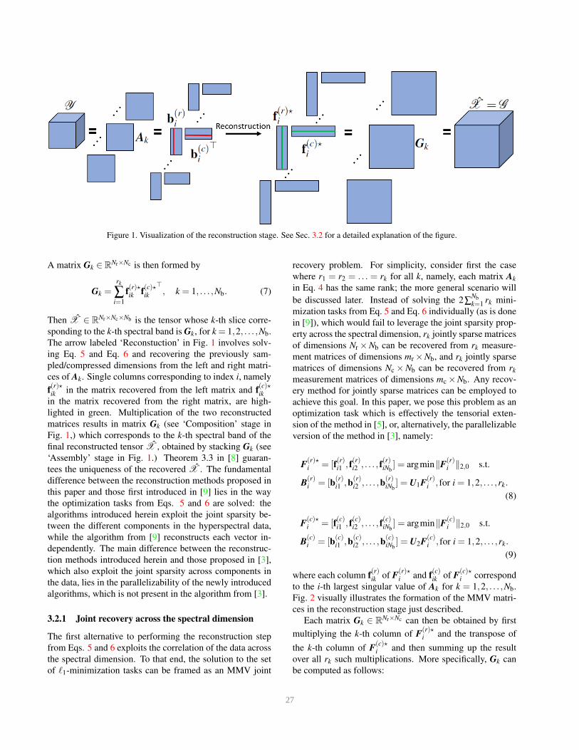
Figure 1. Visualization of the reconstruction stage. See Sec. 3.2 for a detailed explanation of the figure.

A matrix Gk ∈ RNr×Nc is then formed by

Gk =rk

∑i=1

f(r)⋆ik f

(c)⋆ik

⊤, k = 1, . . . ,Nb. (7)

Then X ∈ RNr×Nc×Nb is the tensor whose k-th slice corre-

sponding to the k-th spectral band is Gk, for k = 1,2, . . . ,Nb.

The arrow labeled ‘Reconstuction’ in Fig. 1 involves solv-

ing Eq. 5 and Eq. 6 and recovering the previously sam-

pled/compressed dimensions from the left and right matri-

ces of Ak. Single columns corresponding to index i, namely

f(r)⋆ik in the matrix recovered from the left matrix and f

(c)⋆ik

in the matrix recovered from the right matrix, are high-

lighted in green. Multiplication of the two reconstructed

matrices results in matrix Gk (see ‘Composition’ stage in

Fig. 1,) which corresponds to the k-th spectral band of the

final reconstructed tensor X , obtained by stacking Gk (see

‘Assembly’ stage in Fig. 1.) Theorem 3.3 in [8] guaran-

tees the uniqueness of the recovered X . The fundamental

difference between the reconstruction methods proposed in

this paper and those first introduced in [9] lies in the way

the optimization tasks from Eqs. 5 and 6 are solved: the

algorithms introduced herein exploit the joint sparsity be-

tween the different components in the hyperspectral data,

while the algorithm from [9] reconstructs each vector in-

dependently. The main difference between the reconstruc-

tion methods introduced herein and those proposed in [3],

which also exploit the joint sparsity across components in

the data, lies in the parallelizability of the newly introduced

algorithms, which is not present in the algorithm from [3].

3.2.1 Joint recovery across the spectral dimension

The first alternative to performing the reconstruction step

from Eqs. 5 and 6 exploits the correlation of the data across

the spectral dimension. To that end, the solution to the set

of ℓ1-minimization tasks can be framed as an MMV joint

recovery problem. For simplicity, consider first the case

where r1 = r2 = . . . = rk for all k, namely, each matrix Ak

in Eq. 4 has the same rank; the more general scenario will

be discussed later. Instead of solving the 2∑Nbk=1 rk mini-

mization tasks from Eq. 5 and Eq. 6 individually (as is done

in [9]), which would fail to leverage the joint sparsity prop-

erty across the spectral dimension, rk jointly sparse matrices

of dimensions Nr ×Nb can be recovered from rk measure-

ment matrices of dimensions mr ×Nb, and rk jointly sparse

matrices of dimensions Nc ×Nb can be recovered from rk

measurement matrices of dimensions mc ×Nb. Any recov-

ery method for jointly sparse matrices can be employed to

achieve this goal. In this paper, we pose this problem as an

optimization task which is effectively the tensorial exten-

sion of the method in [5], or, alternatively, the parallelizable

version of the method in [3], namely:

F(r)⋆i = [f

(r)i1 , f

(r)i2 , . . . , f

(r)iNb

] = argmin‖F(r)i ‖2,0 s.t.

B(r)i = [b

(r)i1 ,b

(r)i2 , . . . ,b

(r)iNb

] = U1F(r)i , for i = 1,2, . . . ,rk.

(8)

F(c)⋆i = [f

(c)i1 , f

(c)i2 , . . . , f

(c)iNb

] = argmin‖F(c)i ‖2,0 s.t.

B(c)i = [b

(c)i1 ,b

(c)i2 , . . . ,b

(c)iNb

] = U2F(c)i , for i = 1,2, . . . ,rk.

(9)

where each column f(r)ik of F

(r)⋆i and f

(c)ik of F

(c)⋆i correspond

to the i-th largest singular value of Ak for k = 1,2, . . . ,Nb.

Fig. 2 visually illustrates the formation of the MMV matri-

ces in the reconstruction stage just described.

Each matrix Gk ∈ RNr×Nc can then be obtained by first

multiplying the k-th column of F(r)⋆i and the transpose of

the k-th column of F(c)⋆i and then summing up the result

over all rk such multiplications. More specifically, Gk can

be computed as follows:

27

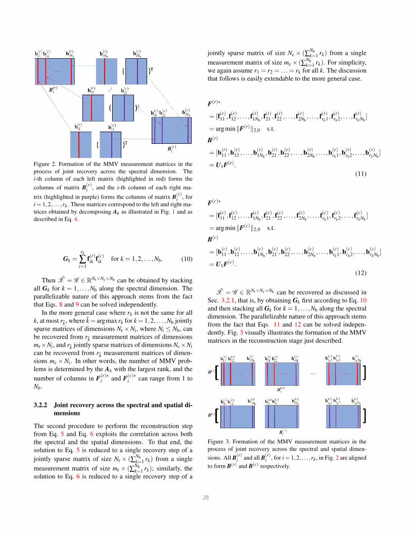
Figure 2. Formation of the MMV measurement matrices in the

process of joint recovery across the spectral dimension. The

i-th column of each left matrix (highlighted in red) forms the

columns of matrix B(r)i , and the i-th column of each right ma-

trix (highlighted in purple) forms the columns of matrix B(r)i , for

i = 1,2, . . . ,rk. These matrices correspond to the left and right ma-

trices obtained by decomposing Ak as illustrated in Fig. 1 and as

described in Eq. 4.

Gk =rk

∑i=1

f(r)ik f

(c)ik for k = 1,2, . . . ,Nb. (10)

Then X = G ∈ RNr×Nc×Nb can be obtained by stacking

all Gk for k = 1, . . . ,Nb along the spectral dimension. The

parallelizable nature of this approach stems from the fact

that Eqs. 8 and 9 can be solved independently.

In the more general case where rk is not the same for all

k, at most rk, where k= argmaxrk for k= 1,2, . . . ,Nb jointly

sparse matrices of dimensions Nr ×Ni, where Ni ≤ Nb, can

be recovered from rk measurement matrices of dimensions

mr×Ni, and rk jointly sparse matrices of dimensions Nc×Ni

can be recovered from rk measurement matrices of dimen-

sions mc ×Ni. In other words, the number of MMV prob-

lems is determined by the Ak with the largest rank, and the

number of columns in F(r)⋆i and F

(c)⋆i can range from 1 to

Nb.

3.2.2 Joint recovery across the spectral and spatial di-

mensions

The second procedure to perform the reconstruction step

from Eq. 5 and Eq. 6 exploits the correlation across both

the spectral and the spatial dimensions. To that end, the

solution to Eq. 5 is reduced to a single recovery step of a

jointly sparse matrix of size Nr × (∑Nbk=1 rk) from a single

measurement matrix of size mr × (∑Nbk=1 rk); similarly, the

solution to Eq. 6 is reduced to a single recovery step of a

jointly sparse matrix of size Nc × (∑Nbk=1 rk) from a single

measurement matrix of size mc × (∑Nbk=1 rk). For simplicity,

we again assume r1 = r2 = . . .= rk for all k. The discussion

that follows is easily extendable to the more general case.

F(r)⋆

= [f(r)11 , f

(r)12 , . . . , f

(r)1Nb

, f(r)21 , f

(r)22 , . . . , f

(r)2Nb

, . . . , f(r)rk1, f

(r)rk2, . . . , f

(r)rkNb

]

= argmin‖F(r)‖2,0 s.t.

B(r)

= [b(r)11 ,b

(r)12 , . . . ,b

(r)1Nb

,b(r)21 ,b

(r)22 , . . . ,b

(r)2Nb

, . . . ,b(r)rk1,b

(r)rk2, . . . ,b

(r)rkNb

]

= U1F(r).

(11)

F(c)⋆

= [f(c)11 , f

(c)12 , . . . , f

(c)1Nb

, f(c)21 , f

(c)22 , . . . , f

(c)2Nb

, . . . , f(c)rk1, f

(c)rk2, . . . , f

(c)rkNb

]

= argmin‖F(c)‖2,0 s.t.

B(c)

= [b(c)11 ,b

(c)12 , . . . ,b

(c)1Nb

,b(c)21 ,b

(c)22 , . . . ,b

(c)2Nb

, . . . ,b(c)rk1,b

(c)rk2, . . . ,b

(c)rkNb

]

= U1F(c).

(12)

X = G ∈ RNr×Nc×Nb can be recovered as discussed in

Sec. 3.2.1, that is, by obtaining Gk first according to Eq. 10

and then stacking all Gk for k = 1, . . . ,Nb along the spectral

dimension. The parallelizable nature of this approach stems

from the fact that Eqs. 11 and 12 can be solved indepen-

dently. Fig. 3 visually illustrates the formation of the MMV

matrices in the reconstruction stage just described.

Figure 3. Formation of the MMV measurement matrices in the

process of joint recovery across the spectral and spatial dimen-

sions. All B(r)i and all B

(r)i , for i = 1,2, . . . ,rk, in Fig. 2 are aligned

to form B(r) and B

(c) respectively.

28

4. Experimental results

We tested the performance of the proposed algorithms

both in terms of reconstruction accuracy and execution

time. We compare our results to those achieved by the

method introduced in [15], which we denote SL2,0, and be-

lieve to be state-of-the-art in terms of vectorial only MMV

reconstruction when only imposing the sparsity constraint

on the data to be sensed. In addition, we evaluate the pro-

posed parallelizable methods against the previously pro-

posed serial versions from [3], which we believe to be state-

of-the-art with regards to tensorial MMV reconstruction.

The legends in the figures in this section refer to the pro-

posed first (Sec. 3.2.1) and second (Sec. 3.2.2) variants

of the proposed algorithm as TMMV1P and TMMV2P re-

spectively, which stand for parallelizable Tensorial MMV

exploiting correlation across the spectral dimension, and

across the spectral and spatial dimensions, respectively. We

refer to the serial counterparts from [3] as TMMV1S and

TMMV2S respectively, which stand for serial Tensorial

MMV exploiting correlation across the spectral dimension,

and across the spectral and spatial dimensions, respectively.

In order to test the performance of the algorithms, acqui-

sition and reconstruction of hyperspectral images from the

AVIRIS Yellowstone dataset introduced in [12] was sim-

ulated. The AVIRIS data consists of five calibrated and

corresponding 16-bit raw images acquired over Yellow-

stone, WY in 2006, as well as two additional 12-bit uncal-

ibrated images. Each image is a 512-line scene containing

224 spectral bands. Reconstruction accuracy was measured

in terms of Normalized Mean Squared Error (NMSE) be-

tween the reconstructed and original image, and execution

time was measured in seconds on a Windows 10 machine

with 32GBytes of RAM and an Intel i7 2.60GHz processor.

The implementation of both algorithms was done in Matlab

R2016b. Each data point in every figure corresponds to an

average of ten runs.

In order to keep the computational complexity of the

problem manageable for the SL2,0 algorithm, the hyper-

spectral images were cropped to 32 × 32 pixels and 32

bands. Let n = mr = mc denote the number of measure-

ments along both spatial dimensions of the hyperspectral

image; the entries of the sampling matrices are drawn from

a Gaussian distribution with zero-mean and standard devi-

ation

√

1n. For simplicity, we set the number of measure-

ments for both spatial dimensions to be equal and use the

same sampling matrix for both dimensions (U1 = U2 = U);

that is, the randomly constructed Gaussian matrix U is of

size n× 32 for each mode. Therefore, the sampling ma-

trix for the method in [15] is equivalent to U⊗U of size

n2 × 322, which results in a total number of measurements

of 32n2 across the spectral bands. We refer to n2

322 as the

normalized number of measurements. We vary the normal-

ized number of measurements from 0.025 to 0.5 in steps of

0.025.

0 0.1 0.2 0.3 0.4 0.5Normalized number of measurements

0

0.2

0.4

0.6

0.8

1

1.2

NM

SE

TMMV1STMMV2SSL2,0TMMV1PTMMV2P


0

10

20

30

40

50

60

70

Rec

onst

ruct

ion

time

(sec

) TMMV1TMMV2SL2,0TMMV1PTMMV2P


0

0.2

0.4

0.6

0.8

1

1.2

NM

SE



10

20

30

40

50

60

70

Rec

onst

ruct

ion

time

(sec



0.2

0.4

0.6

0.8

1

1.2

NM

SE



10

20

30

40

50

60

70

80

Rec

onst

ruct

ion

time

(sec



0.6

0.7

0.8

0.9

1

1.1

1.2

NM

SE



10

20

30

40

50

60

70

80

Rec

onst

ruct

ion

time

(sec


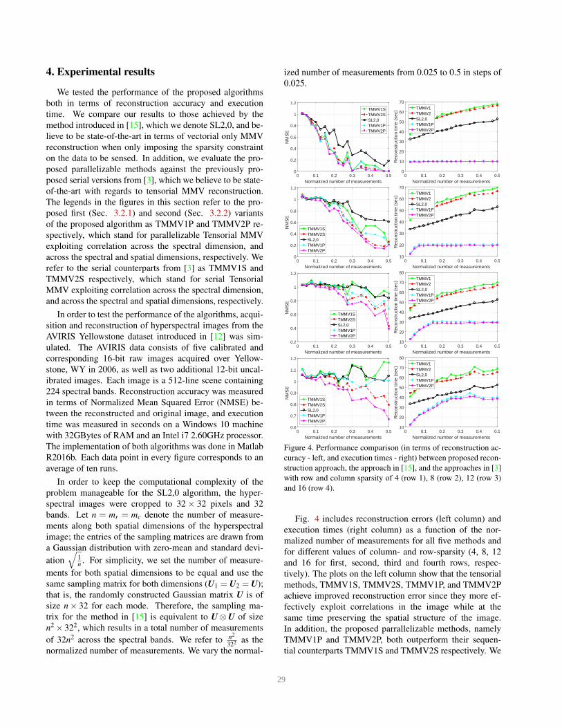
Figure 4. Performance comparison (in terms of reconstruction ac-

curacy - left, and execution times - right) between proposed recon-

struction approach, the approach in [15], and the approaches in [3]

with row and column sparsity of 4 (row 1), 8 (row 2), 12 (row 3)

and 16 (row 4).

Fig. 4 includes reconstruction errors (left column) and

execution times (right column) as a function of the nor-

malized number of measurements for all five methods and

for different values of column- and row-sparsity (4, 8, 12

and 16 for first, second, third and fourth rows, respec-

tively). The plots on the left column show that the tensorial

methods, TMMV1S, TMMV2S, TMMV1P, and TMMV2P

achieve improved reconstruction error since they more ef-

fectively exploit correlations in the image while at the

same time preserving the spatial structure of the image.

In addition, the proposed parrallelizable methods, namely

TMMV1P and TMMV2P, both outperform their sequen-

tial counterparts TMMV1S and TMMV2S respectively. We

29

believe the reasons for this performance improvement are

twofold. In terms of reconstruction error, the serial ver-

sion reconstructs two tensorial modes sequentially, which

transfers the reconstruction error in the first tensor mode to

the next stage, causing the errors to accumulate and possi-

bly magnify between stages. In contrast, the parallelizable

TMMV methods decouple the reconstruction of the two ten-

sor modes, so there is no error accummulation across the re-

constructed modes. In terms of computational complexity,

the proposed approach benefits from the reduced number

of reconstruction problems that are solved, which is deter-

mined by the rank of the measurement matrices. We note

that, as its name indicates, the parallelizable approach can

benefit from multi-threading; however, for comparison pur-

poses, we implemented and tested a non-parallelized ver-

sion of the algorithm. The results show that despite its su-

periority, there is significant room for improvement for the

parallelizable version of the algorithm when multiple pro-

cessing cores are available, regardless of the rank of the

original signal.

The fact that TMMV2P is generally superior to

TMMV1P shows that exploiting spatial and spectral corre-

lations together leads to a slight gain in both computational

efficiency and accuracy. Both TMMV1P and TMMV2P are

faster than SL2,0 and their sequential counterparts since the

measurement matrix for the tensorial approaches has lower

dimensionality than its vectorial counterpart. As expected,

as the number of measurements being acquired increases,

reconstruction error improves at a slight cost of computa-

tional complexity. We note that, in contrast with the re-

sults reported in [3], SL2,0 is more computationally effi-

cient than both TMMV1S and TMMV2S. We believe this

is because the experimental validation in [3] evaluated the

performance of the algorithms on the reconstruction of 3-

channel color images, which seems to indicate that SL2,0

scales better as the number of channels grows.

As stated, the NMSE reported in Fig. 4 for each data

point is an average across 10 trials; however, some tasks im-

pose constraints on the largest NMSE that can be allowed.

Consequently, additional insight into the reconstruction per-

formance of the algorithms can be gained from evaluat-

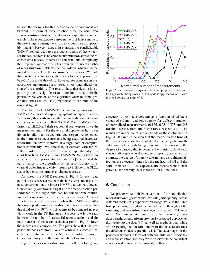
ing and comparing reconstruction success rates. A recon-

struction is deemed successful when the NMSE is smaller

than some predetermined threshold; in this case, we set that

threshold to 1× 10−3, which seems to be standard in pre-

vious work in the CS literature. Success rate is the ratio

between the number of successful reconstructions and the

total number of trials for each data point. Fig. 5 shows

the success rate comparison. The plots show that the pro-

posed methods are more likely to achieve a successful re-

construction that satisfies the NSP constraint according to

CS methodology with the same number of measurements.

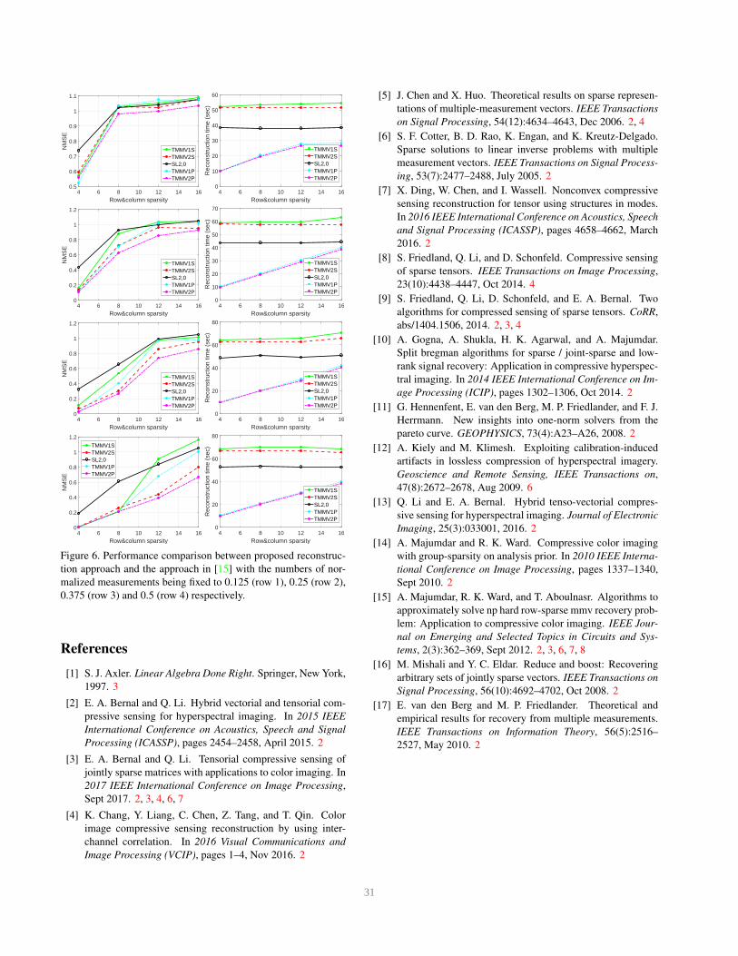
Fig. 6 includes reconstruction errors (left column) and


0

0.2

0.4

0.6

0.8

1

Rec

onst

ruct

ion

succ

ess

rate TMMV1S

TMMV2SSL2,0TMMV1PTMMV2P

Figure 5. Success rate comparison between proposed reconstruc-

tion approach, the approach in [15], and the approaches in [3] with

row and column sparsity of 4.

execution times (right column) as a function of different

values of column- and row-sparsity for different numbers

of normalized measurements (0.125, 0.25, 0.375 and 0.5

for first, second, third and fourth rows, respectively). The

results are indicative of similar trends as those observed in

Fig. 4. It can also be seen that the reconstruction time of

the parallelizable methods, while always being the small-

est among all methods being compared, increases with the

degree of sparsity; this is because the matrix rank of each

spectral slice grows as the degree of sparsity increases. In

contrast, the degree of sparsity doesnt have a significant ef-

fect on the execution times for the method in [15] and the

serial methods [3]. As expected, the reconstruction error

grows as the sparsity level increases for all methods.

5. Conclusion

We proposed two different variants of a parallelizable

reconstruction algorithm that exploits joint sparsity across

different modes of a hyperspectral image while at the same

time preserving its high-dimensional nature throughout the

sampling and reconstruction stages of a novel CS frame-

work. We demonstrated empirically that the newly intro-

duced methods outperform previously proposed approaches

that vectorize the data [15], as well as methods that, while

still respecting the tensorial nature of the data, reconstruct

the different modes sequentially [3]. The advantages of the

proposed methods in terms of both computational efficiency

and reconstruction accuracy were observed to be consistent

across a wide range of experimental settings.

30

4 6 8 10 12 14 16Row&column sparsity

0.5

0.6

0.7

0.8

0.9

1

1.1

NM

SE



0

10

20

30

40

50

60

Rec

onst

ruct

ion

time

(sec

)



0

0.2

0.4

0.6

0.8

1

1.2

NM

SE



0

10

20

30

40

50

60

70R

econ

stru

ctio

n tim

e (s

ec)



0

0.2

0.4

0.6

0.8

1

1.2

NM

SE



0

20

40

60

80

Rec

onst

ruct

ion

time

(sec

)



0

0.2

0.4

0.6

0.8

1

1.2

NM

SE



0

20

40

60

80

Rec

onst

ruct

ion

time

(sec

)


Figure 6. Performance comparison between proposed reconstruc-

tion approach and the approach in [15] with the numbers of nor-

malized measurements being fixed to 0.125 (row 1), 0.25 (row 2),

0.375 (row 3) and 0.5 (row 4) respectively.

References

[1] S. J. Axler. Linear Algebra Done Right. Springer, New York,

1997. 3

[2] E. A. Bernal and Q. Li. Hybrid vectorial and tensorial com-

pressive sensing for hyperspectral imaging. In 2015 IEEE

International Conference on Acoustics, Speech and Signal

Processing (ICASSP), pages 2454–2458, April 2015. 2

[3] E. A. Bernal and Q. Li. Tensorial compressive sensing of

jointly sparse matrices with applications to color imaging. In

2017 IEEE International Conference on Image Processing,

Sept 2017. 2, 3, 4, 6, 7

[4] K. Chang, Y. Liang, C. Chen, Z. Tang, and T. Qin. Color

image compressive sensing reconstruction by using inter-

channel correlation. In 2016 Visual Communications and

Image Processing (VCIP), pages 1–4, Nov 2016. 2

[5] J. Chen and X. Huo. Theoretical results on sparse represen-

tations of multiple-measurement vectors. IEEE Transactions

on Signal Processing, 54(12):4634–4643, Dec 2006. 2, 4

[6] S. F. Cotter, B. D. Rao, K. Engan, and K. Kreutz-Delgado.

Sparse solutions to linear inverse problems with multiple

measurement vectors. IEEE Transactions on Signal Process-

ing, 53(7):2477–2488, July 2005. 2

[7] X. Ding, W. Chen, and I. Wassell. Nonconvex compressive

sensing reconstruction for tensor using structures in modes.

In 2016 IEEE International Conference on Acoustics, Speech

and Signal Processing (ICASSP), pages 4658–4662, March

2016. 2

[8] S. Friedland, Q. Li, and D. Schonfeld. Compressive sensing

of sparse tensors. IEEE Transactions on Image Processing,

23(10):4438–4447, Oct 2014. 4

[9] S. Friedland, Q. Li, D. Schonfeld, and E. A. Bernal. Two

algorithms for compressed sensing of sparse tensors. CoRR,

abs/1404.1506, 2014. 2, 3, 4

[10] A. Gogna, A. Shukla, H. K. Agarwal, and A. Majumdar.

Split bregman algorithms for sparse / joint-sparse and low-

rank signal recovery: Application in compressive hyperspec-

tral imaging. In 2014 IEEE International Conference on Im-

age Processing (ICIP), pages 1302–1306, Oct 2014. 2

[11] G. Hennenfent, E. van den Berg, M. P. Friedlander, and F. J.

Herrmann. New insights into one-norm solvers from the

pareto curve. GEOPHYSICS, 73(4):A23–A26, 2008. 2

[12] A. Kiely and M. Klimesh. Exploiting calibration-induced

artifacts in lossless compression of hyperspectral imagery.

Geoscience and Remote Sensing, IEEE Transactions on,

47(8):2672–2678, Aug 2009. 6

[13] Q. Li and E. A. Bernal. Hybrid tenso-vectorial compres-

sive sensing for hyperspectral imaging. Journal of Electronic

Imaging, 25(3):033001, 2016. 2

[14] A. Majumdar and R. K. Ward. Compressive color imaging

with group-sparsity on analysis prior. In 2010 IEEE Interna-

tional Conference on Image Processing, pages 1337–1340,

Sept 2010. 2

[15] A. Majumdar, R. K. Ward, and T. Aboulnasr. Algorithms to

approximately solve np hard row-sparse mmv recovery prob-

lem: Application to compressive color imaging. IEEE Jour-

nal on Emerging and Selected Topics in Circuits and Sys-

tems, 2(3):362–369, Sept 2012. 2, 3, 6, 7, 8

[16] M. Mishali and Y. C. Eldar. Reduce and boost: Recovering

arbitrary sets of jointly sparse vectors. IEEE Transactions on

Signal Processing, 56(10):4692–4702, Oct 2008. 2

[17] E. van den Berg and M. P. Friedlander. Theoretical and

empirical results for recovery from multiple measurements.

IEEE Transactions on Information Theory, 56(5):2516–

2527, May 2010. 2

31

An Algorithm for Parallel Reconstruction of Jointly...

Documents

Transcript of An Algorithm for Parallel Reconstruction of Jointly...