1

An Agent-Based Test Bed Study ofWholesale Power Market Performance Measures

Abhishek Somani and Leigh Tesfatsion, Member, IEEE

Abstract—Wholesale power markets operating over trans-mission grids subject to congestion have distinctive featuresthat complicate the detection of market power and operationalinefficiency. This study uses a wholesale power market test bedwith strategically learning traders to experimentally test theextent to which market performance measures commonly usedfor other industries are informative for the dynamic operationof restructured wholesale power markets. Examined measuresinclude the Herfindahl-Hirschman Index (HHI), the LernerIndex, the Residual Supply Index, the Relative Market AdvantageIndex, and the Operational Efficiency Index. It is also shown thatthe objective function commonly used to manage these marketsdeviates systematically from the standard economic measure ofmarket efficiency when grid congestion is present.

Index Terms—AMES Wholesale Power Market Test Bed;Agent-based modeling; Restructured wholesale power markets;Dynamic market performance; HHI; Lerner Index; ResidualSupply Index; Relative Market Advantage Index; OperationalEfficiency Index

I. INTRODUCTION

THe U.S. electric power industry is currently undergoingsubstantial changes in both its structure (ownership and

technology aspects) and its architecture (operational and over-sight aspects). These changes involve attempts to move theindustry away from highly regulated markets with adminis-tered cost-based pricing and towards competitive markets inwhich prices more fully reflect supply and demand forces.

The goal of these changes is to provide industry participantswith better incentives to control costs and introduce innova-tions. The process of enacting and implementing policies andlaws to bring about these changes has come to be known asrestructuring.

This restructuring process has been controversial. The melt-down in the restructured California wholesale power marketin the summer of 2000 has shown what can happen whenmarket mechanisms with complicated incentive structures areimplemented without sufficient pre-testing. Following the Cal-ifornia crisis, numerous energy researchers have argued theneed to combine sound physical understanding of electricpower and transmission grid operation with economic analysisof incentives in order to develop electricity markets with goodreal-world performance characteristics.

Latest revision: 2 October 2008. This study is scheduled to appear in aspecial issue of the IEEE Computational Intelligence Magazine (Vol. 3, No. 4,November 2008, 56-72). It has been supported in part by the National ScienceFoundation under Grant NSF-0527460.

Ahishek Somani (somaniabhishek@yahoo.com) and Leigh Tesfatsion (cor-responding author: tesfatsi@iastate.edu), Economics Department, Iowa StateUniversity, Ames, IA 50011 USA.

Many commercially available packages for power systemanalysis now incorporate components critical for the simu-lation of restructured electricity markets (e.g. optimal powerflow solvers). However, these packages have three majordrawbacks.

First, the critical effect of incentives on human participantbehaviors is typically not addressed. Second, the proprietarynature of these packages generally prevents users from gaininga complete and accurate understanding of what has been im-plemented, restricts the ability of users to experiment with newsoftware features, and hinders users from tailoring software tospecific needs. Third, the concern for commercial applicabilityto large-scale real-world systems makes these packages cum-bersome to use for research, teaching, and training purposesrequiring intensive experimentation and sensitivity analyses.

In response to these concerns, a group of researchers atIowa State University has been working to develop the AMESWholesale Power Market Test Bed.1 AMES is an agent-basedcomputational laboratory suitable for studying the dynamicperformance of restructured wholesale power markets in amanner that addresses both economic and engineering con-cerns. A key aspect of the AMES project is the release ofAMES as open-source software to encourage interdisciplinarycommunication and cumulative enhancements.

AMES incorporates core elements of a wholesale powermarket design recommended by the U.S. Federal Energy Reg-ulatory Commission (FERC) in an April 2003 White Paper [6].This design recommends the operation of wholesale powermarkets by Independent System Operators (ISOs) or RegionalTransmission Organizations (RTOs) using locational marginalprices (LMPs) to price energy by the location and timing ofits injection into or withdrawal from the transmission grid.

As shown in Fig. 1, variants of FERC’s proposed wholesalepower market design have now been adopted in many regionsof the U.S. These regions include New England (ISO-NE),New York (NYISO), the mid-atlantic states (PJM), the mid-west (MISO), the southwest (SPP), and California (CAISO).According to Joskow [7], over 50% of generating capacityin the U.S. is now operating under some variant of FERC’smarket design.

AMES models electric power sellers (generation companies)with learning capabilities interacting over time with elec-

1Detailed descriptions of AMES can be found in refs. ([1], [2], [3], [4]).AMES is an acronym for Agent-based Modeling of Electricity Systems. Thefirst version of AMES was released as an open-source Java software packageat the IEEE PES General Meeting in June 2007. Downloads, manuals, andtutorial information for all AMES version releases to date can be accessed atthe AMES homepage [5].

2

Fig. 1. Energy regions operating under variants of FERC’s market design

tric power buyers (load-serving entities) in an ISO-managedwholesale power market. This market operates over an ACtransmission grid subject to congestion. The ISO managescongestion on the grid by means of LMPs derived fromoptimal power flow solutions.

This study explores the potential usefulness of test beds suchas AMES for practical energy policy concerns. Specifically, weuse AMES to experimentally test the extent to which marketperformance measures commonly used for other industriesare informative for the dynamic operation of restructuredwholesale power markets.

In particular, we focus on the measurement of “seller marketpower” and “market efficiency” relative to a “competitiveequilibrium ” benchmark. Competitive equilibrium is said tohold for a market when all traders take prices as given inthe formulation of their demands and supplies and the marketprice is then set to equate total market demand to total marketsupply. Seller market power refers to the ability of a seller toprofitably raise the market price of a good relative to compet-itive equilibrium conditions. Market efficiency measures thedegree to which the total net surplus (earnings) secured bysellers and buyers through actual market operations matchesthe maximum total net surplus that sellers and buyers wouldsecure under competitive equilibrium conditions.

The organization of this study is as follows. The mainfeatures of the AMES test bed are outlined in Section II.In Section III we elaborate on several special factors com-plicating the detection and prevention of seller market powerand the measurement and attainment of market efficiency inrestructured wholesale power markets. In particular, we showthat the standard ISO optimal power flow objective functionused to manage these markets deviates systematically fromthe standard economic measure for market efficiency whengrid congestion is present.

In Section IV we provide careful definitions for the spe-cific seller market power and market efficiency measuresto be experimentally examined in this study. We start withtwo commonly used measures for seller market power, theHerfindahl-Hirschman Index (HHI) and the Lerner Index. Wethen present the Residual Supply Index recently developedby CAISO researchers as a test for seller market power inwholesale power markets. We next explain the Relative MarketAdvantage Index, a market performance measure developed byNicolaisen et al. [8] as a necessary indicator for seller market

Fig. 2. AMES test bed architecture

Fig. 3. AMES GenCo: A cognitive agent with learning capabilities

power. Finally, we examine a measure for efficient marketoperations referred to as the Operational Efficiency Index.

Section V sets out a simple experimental design permittingcomparisons of the strengths and weaknesses of each of thesemeasures relative to its intended purpose. Section VI presentssome of our main experimental findings to date.

Power markets are critically important systems for nationalwelfare and security, but they are also inherently complicatedto understand. In keeping with the purposes of this specialissue, every effort is made below to keep equations to a min-imum. However, as an aid to interested readers, pointers aregiven to supporting works where more technical discussionscan be found.

II. THE AMES TEST BED (VERSION 2.01)

A. Overview

AMES(V2.01) incorporates, in simplified form, core fea-tures of the wholesale power market design proposed by theU.S. FERC [6]; see Fig. 2. A detailed description of thesefeatures can be found in materials provided at the AMEShomepage [5].

Below is a summary description of the logical flow of eventsin the AMES(V2.01) wholesale power market:• The AMES wholesale power market operates over an

AC transmission grid starting on day 1 and continuingthrough a user-specified maximum day (unless terminated

3

Fig. 4. AMES GenCos use stochastic reinforcement learning to determinethe supply offers they report to the ISO for the day-ahead market.

earlier in accordance with a user-specified stopping rule).Each day D consists of 24 successive hours H = 00,01,...,23.

• The AMES wholesale power market includes an Indepen-dent System Operator (ISO) and a collection of energytraders consisting of Load-Serving Entities (LSEs) andGeneration Companies (GenCos) distributed across thebusses of the transmission grid. Each of these entities isimplemented as a software program encapsulating bothmethods and data; see, e.g., the schematic depiction of aGenCo in Fig. 3

• The objective of the ISO is the reliable attainment ofappropriately constrained operational efficiency for thewholesale power market, i.e., the maximization of buyerand seller total net surplus (earnings) subject to genera-tion and transmission constraints.

• In an attempt to attain this objective, the ISO undertakesthe daily operation of a day-ahead market settled bymeans of locational marginal pricing (LMP), i.e., thedetermination of prices for electric power in accordancewith the location and timing of its injection into, orwithdrawal from, the transmission grid. Roughly stated,a locational marginal price at any particular transmissiongrid bus is the least cost to the system of servicingdemand for one additional megawatt (MW) of electricpower at that bus.2

• The objective of each LSE is to secure power for itsdownstream (retail) customers. During the morning ofeach day D, each LSE reports a demand bid to the ISOfor the day-ahead market for day D+1. Each demand bidconsists of two parts: a fixed demand bid (i.e., a 24-hourload profile); and 24 price-sensitive demand bids (one foreach hour), each consisting of a linear demand functiondefined over a purchase capacity interval. LSEs have no

2In reality, LMPs are shadow prices for “nodal balance constraints”constituting part of the constraint set of optimal power flow problems and arederived as derivatives of the optimized power flow objective function withrespect to particular types of perturbations of these constraints. Moreover,these nodal balance constraints are imposed at “pricing nodes” that mightnot correspond to actual physical bus locations on the grid. For expositionalsimplicity, throughout this study we use the standard engineering short-handdescription for LMPs as valuations for single-unit increases in demand andwe treat pricing nodes as coincident with transmission grid busses. For a morerigorous explanation and derivation of LMPs, see [2].

learning capabilities; LSE demand bids are user-specifiedat the beginning of each simulation run.

• The objective of each GenCo is to secure for itselfthe highest possible net earnings each day. During themorning of each day D, each GenCo i uses its currentaction choice probabilities to choose a supply offer fromits action domain ADi to report to the ISO for use in all24 hours of the day-ahead market for day D+1.3

• Each supply offer in ADi consists of a linear marginalcost function defined over an operating capacity interval.GenCo i’s ability to vary its choice of supply offersfrom ADi permits it to adjust the ordinate/slope of itsreported marginal cost function and/or the upper limit ofits reported operating capacity interval in an attempt toincrease its daily net earnings.

• After receiving demand bids from LSEs and supply offersfrom GenCos during the morning of day D, the ISOdetermines and publicly reports hourly power supplycommitments and LMPs for the day-ahead market forday D+1 as the solution to hourly bid/offer-based DCoptimal power flow (DC-OPF) problems. Transmissiongrid congestion is managed by the inclusion of congestioncost components in LMPs.

• At the end of each day D, the ISO settles all of thecommitments for the day-ahead market for day D+1 onthe basis of the LMPs for the day-ahead market for dayD+1.

• At the end of each day D, each GenCo i uses stochasticreinforcement learning to update the action choice proba-bilities currently assigned to the supply offers in its actiondomain ADi taking into account its day-D settlementpayment (“reward”). In particular, as depicted in Fig. 4, ifthe supply offer reported by GenCo i on day D results in arelatively good reward, GenCo i increases the probabilityof choosing this supply offer on day D+1, and conversely.

• There are no system disturbances (e.g., weather changes)or shocks (e.g., forced generation outages or line out-ages). Consequently, the binding financial contracts deter-mined in the day-ahead market are carried out as plannedand traders have no need to engage in real-time (spot)market trading.

• Each LSE and GenCo has an initial holding of moneythat changes over time as it accumulates earnings andlosses.

• There is no entry of traders into, or exit of tradersfrom, the wholesale power market. LSEs and GenCosare currently allowed to go into debt (negative moneyholdings) without penalty or forced exit.

The activities of the ISO on a typical day D are depictedin Fig. 5. The overall dynamical flow of activities in the

3In the MISO [9], GenCos each day are actually permitted to report aseparate supply offer for each hour of the day-ahead market. In order tosimplify the learning problem for GenCos, the current version of AMESrestricts GenCos to the daily reporting of only one supply offer for the day-ahead market. Interestingly, the latter restriction is imposed on GenCos bythe ISO-NE [10] in its particular implementation of FERC’s market design.Baldick and Hogan [11, pp. 18-20] conjecture that imposing such limits onthe ability of GenCos to report distinct hourly supply offers could reduce theirability to exercise seller market power.

4

Fig. 5. AMES ISO activities during a typical day D

Fig. 6. Illustration of AMES dynamics on a typical day D in the absenceof system disturbances or shocks for the special case of a 5-bus grid

wholesale power market on a typical day D in the absenceof system disturbances or shocks is depicted in Fig. 6.

III. MEASUREMENT CONUNDRUMS FOR POWER MARKETS

A. Detection of Seller Market Power

Although the exercise of seller market power in restructuredwholesale power markets can have substantial adverse effectson the efficiency, reliability, and fairness of market operations,it is difficult to construct measures for its reliable detection.Excellent discussions elaborating some of the reasons for thiscan be found in Borenstein et al. [12], Sheffrin et al. [13],Stoft [14, Chapter 4], and Twomey et al. [15]. Here we brieflyreview the key issues.

On the one hand, the complexity of the rules and regula-tions governing market operations in restructured wholesalepower markets creates opportunities for GenCos to game the

system to their advantage through strategic behaviors, eitherindividually or in tacit collusion. These strategic behaviors taketwo main forms: economic withholding of capacity througha reporting of higher-than-true marginal costs; and physicalwithholding of capacity.

Economic withholding of capacity can induce higher pricesfor cleared supply as well as out-of-merit-order dispatch,i.e., more expensive generation dispatched in place of lessexpensive generation. This results in inefficient (and politicallyimportant) transfers of wealth away from LSEs and theirdownstream (retail) consumers and towards GenCos.

Physical withholding of capacity can induce higher pricesfor the remaining offered capacity and hence higher netearnings for GenCos that withhold only a portion of theircapacities. It can also result in out-of-merit-order dispatch. Inaddition, however, physical withholding of capacity increasesthe chances of inadequacy events in which offered capacity isinsufficient to meet total fixed demand, forcing ISOs to takespecial actions to avoid the breakdown of power flow on thegrid.

In short, strategic withholding results in distorted pricesignals as well as the possible need for special non-marketdispatch. This hinders the efficient and fair use of existing re-sources as well as the proper assessment of future transmissionand generation investment needs.

On the other hand, the physical laws governing powerflow on transmission grids mean that these grids are stronglyconnected networks. Injections or withdrawals of power at onelocation on the grid can have substantial effects on branchflows and bus sensititivies at distant locations. In particular,if an injection of power at a particular grid location leads togrid congestion, this will cause at least some separation ofLMPs across the grid. Indeed, as explained more carefullyin Subsection III-B, under congested conditions LMPs canstrictly exceed the marginal cost of each marginal GenCo atthe system operating point, despite the complete absence ofany deliberate exercise of seller market power.

Alternatively, a change in the pattern of grid congestion cancause dramatic discontinous changes in LMP levels even if theoverall number of congested branches remains the same. Forexample, a load pocket can suddenly emerge in which a GenCoeffectively becomes a high-priced monopolist with respectto the demand for power in its local area because outsidepower cannot be transported into this local area. In standardeconomic terminology, the energy market has segmented intosubmarkets, and the electric power quantities offered for sale atlocations within distinct submarkets now effectively representdistinct goods supporting a distinct array of prices.

Standard economic measures for seller market power havenot been designed with these complex effects in mind. Con-sequently, their usefulness for the detection of seller marketpower in restructured wholesale power markets is not clear.

B. Measurement of Market Efficiency

The standard economic measurement of “market efficiency”also has to be carefully reconsidered for restructured wholesalepower markets. Market efficiency means there are no wasted

5

Fig. 7. Illustration of a competitive equilibrium (Q*,P*) = (5,$65) withcorresponding calculations for net buyer and seller surplus. The range of allpossible competitive equilibria is given by Q*=5 and $60 ≤ P ∗ ≤ $70.

resources. Economists identify two types of wastage: (1)physical wastage, in the sense that some valued units ofresource remain unused; and (2) wastage of value, in the sensethat some units of resource are not being used by those whovalue them most.

Economists measure the efficiency of a market in terms ofthe “total net surplus” attained by buyers and sellers. Netbuyer surplus is defined to be the maximum amount thata buyer would have been willing to pay for a quantity ofgoods q minus the actual payment that the buyer makes forq. Similarly, net seller surplus is defined to be the paymentreceived by a seller for the sale of a quantity of goods q minusthe minimum payment the seller would have been willing toaccept in payment for q. The total net surplus (TNS) attained ina market M during a specified time period T is then definedto be the sum of the net surplus attained by all buyers andsellers in M during T.

Market efficiency is said to be achieved in a market if TNSis maximized, since wastage of resources is then minimized.In standard textbook market settings, TNS is maximized incompetitive equilibrium, that is, when all buyers and sellersin the market take prices as given in the formulation of theirdemands and supplies and the market price P* equates totalmarket demand to total market supply at some common quan-tity level Q*. The equilibrium quantity Q* is the summation ofall of the cleared quantities q∗i supplied by individual sellersi, that is, the quantities q∗i that can be scheduled for purchasebecause for each successive quantity unit the market price liesbetween some buyer’s maximum willingness to pay and theseller’s minimum acceptable price.

See, for example, the depiction of a competitive equilibriumin Fig. 7 with accompanying calculations for net buyer andseller surplus. The demand curve D depicts buyer maximumwillingness to pay for each successive unit demanded, in de-scending order, and the supply curve S depicts seller minimumacceptable sale price for each successive unit supplied, inascending order. The eight quantity units offered for sale mightall belong to a single seller that is not capacity constrained.Alternatively, the eight units could represent units offeredfor sale by different capacity-constrained sellers—e.g., eightdifferent sellers, each capacity-constrained to supply at most

one unit. In either case only five of these units can be cleared incompetitive equilibrium because buyer maximum willingnessto pay drops below seller minimum acceptable sale price forany additionally offered quantity units.

Economists typically equate a seller’s minimum acceptablesale price with its marginal cost. Consequently, economistscommonly test for the maximization of TNS at a point (Q’,P’)by testing whether the market price P’ lies between MC−(Q’)and MC+(Q’), the left-hand and right-hand seller marginalcosts evaluated at the market output level Q’.4 If sellermarginal cost is a well-defined continuous function of Q atQ’, then left-hand and right-hand seller marginal costs coincideat Q’ and this requirement reduces to the standard conditionP’=MC(Q’).5 If P’ exceeds right-hand seller marginal costat Q’, this raises the possibility that additional buyer/sellersurplus could be extracted from the market by the sale ofadditional quantity units. It also raises the possibility thatsellers are exercising market power through the deliberatewithholding of capacity.

Due to network externalities, however, this P/MC test mustbe applied with great caution in restructured wholesale powermarkets operating over transmission grids with congestionmanaged by LMP pricing. To understand why, it is necessaryto consider carefully the constructive derivation of LMPs.

As noted in Section II, the LMP at each bus of thetransmission grid is defined as a right-hand system marginalcost: namely, the least cost to the system of servicing anadditional megawatt (MW) of electric power demand at thatbus. By definition, then, each LMP is determined only bythe marginal GenCos at the system operating point, i.e., bythe GenCos that are capable of supplying additional demandbecause they are currently operating strictly below their uppercapacity limits.

Consequently, as is well understood, the LMP receivedby each individual non-marginal (i.e., capacity-constrained)GenCo for each MW it sells at its operating point can strictlyexceed its left-hand marginal cost.6 The MWs supplied bythese non-marginal GenCos constitute “inframarginal” quan-tity units in the terminology of standard microeconomic theory,similar to the quantity units to the left of Q*=5 in Fig. 7.

What is not as well understood, however, is that an LMP canstrictly exceed the right-hand marginal cost of each marginalGenCo if grid congestion requires out-of-merit-order dispatch.For example, to service an additional MW of demand at some

4Assuming the seller minimum acceptable sale prices in Fig. 7 are marginalcosts, the depicted competitive equilibrium (Q*,P*)=(5,$65) satisfies preciselythis type of requirement, as follows: $60 = MC−(Q*) < P*=$65< MC+(Q*)= $80. A similar requirement can be formulated stating that the marketprice P’ should lie between the left-hand and right-hand expressions forbuyer maximum willingness to pay at Q’. Both of these requirements followfrom the following alternative geometrically-expressed form for the definitionof competitive equilibrium in standard market contexts: A technologicallyfeasible quantity-price combination (Q’,P’) is a competitive equilibrium ifand only if it is an intersection point of the market demand and supply curveswith all vertical and horizontal portions included.

5Marginal cost curves for power markets typically have jump points dueto generation capacity constraints. See Stoft [14, Chapter 1-6] for a carefuldiscussion of marginal cost calculations for power markets.

6The marginal cost curve of a capacity-constrained GenCo goes verticalat its upper capacity limit, implying that the right-hand marginal cost of aGenCo operating at its upper capacity limit is effectively infinite.

6

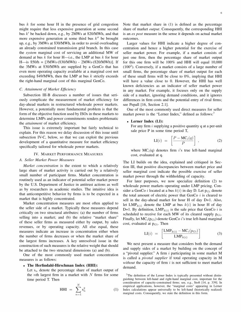
bus k for some hour H in the presence of grid congestionmight require that less expensive generation at some secondbus k′ be backed down, e.g., by 2MWs at $20/MWh, and thatmore expensive generation at some third bus k′′ be broughtup, e.g., by 3MWs at $30/MWh, in order to avoid overloadingan already constrained transmission grid branch. In this casethe system marginal cost of servicing an additional MW ofdemand at bus k for hour H—i.e., the LMP at bus k for hourH—is $50/h = [3MWs·($30/MWh) - 2MWs·($20/MWh)]. Ifthe 3MWs at $30/MWh are supplied by a GenCo that haseven more operating capacity available at a marginal cost notexceeding $49/MWh, then the LMP at bus k strictly exceedsthe right-hand marginal cost of this marginal GenCo.

C. Attainment of Market EfficiencySubsection III-B discusses a number of issues that seri-

ously complicate the measurement of market efficiency forday-ahead markets in restructured wholesale power markets.However, a potentially more fundamental problem is that theform of the objective function used by ISOs in these markets todetermine LMPs and power commitments renders problematicthe attainment of market efficiency.

This issue is extremely important but fairly technical toexplain. For this reason we delay discussion of this issue untilsubsection IV-C, below, so that we can exploit the previousdevelopment of a quantitative measure for market efficiencyspecifically tailored for wholesale power markets.

IV. MARKET PERFORMANCE MEASURES

A. Seller Market Power MeasuresMarket concentration is the extent to which a relatively

large share of market activity is carried out by a relativelysmall number of participant firms. Market concentration isroutinely used as an indicator of potential seller market powerby the U.S. Department of Justice in antitrust actions as wellas by researchers in academic studies. The intuitive idea isthat anticompetitive behavior by firms is to be expected in amarket that is highly concentrated.

Market concentration measures are most often applied tothe seller side of a market. Typically these measures dependcritically on two structural attributes: (a) the number of firmsselling into a market; and (b) the relative “market share”of these seller firms as measured either by output, by salesrevenues, or by operating capacity. All else equal, thesemeasures indicate an increase in concentration either whenthe number of firms decreases or when the market share ofthe largest firms increases. A key unresolved issue in theconstruction of such measures is the relative weight that shouldbe attached to the two structural dimensions (a) and (b).

One of the most commonly used market concentrationmeasures is as follows:• The Herfindahl-Hirschman Index (HHI):

Let sn denote the percentage share of market output ofthe nth largest firm in a market with N firms for sometime period T. Then

HHI =N∑

n=1

s2n (1)

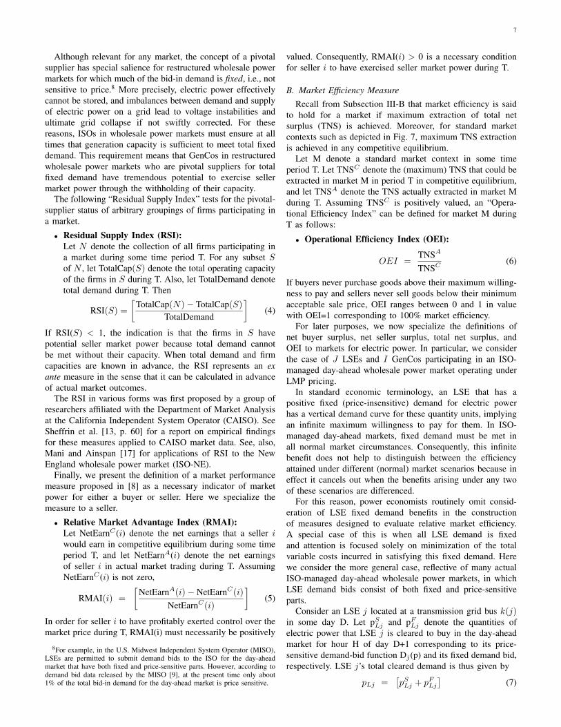
Note that market share in (1) is defined as the percentageshare of market output. Consequently, the corresponding HHIis an ex post measure in the sense it depends on actual marketoutcomes.

Larger values for HHI indicate a higher degree of con-centration and hence a higher potential for the exercise ofseller market power. For example, if a market consists ofjust one firm, then the percentage share of market outputfor this one firm will be 100% and HHI will equal 10,000(1002). Conversely, if a market consists of a large number ofsmall firms, the percentage share of market output for eachof these small firms will be close to 0%, implying that HHIwill have a value close to 0. However, the HHI has wellknown deficiencies as an indicator of seller market powerin any market. For example, it focuses only on the supplyside of a market, ignoring demand conditions, and it ignoresdifferences in firm costs and the potential entry of rival firms;see Pepall [16, Section 2.1].

One of the most commonly used direct measures for sellermarket power is the “Lerner Index,” defined as follows:7

• Lerner Index (LI):For any firm i supplying a positive quantity q at a per-unitsale price P in some time period T,

LI(i) =[P −MCi(q)

P

], (2)

where MCi(q) denotes firm i’s true left-hand marginalcost, evaluated at q.

The LI builds on the idea, explained and critiqued in Sec-tion III, that positive discrepancies between market price andseller marginal cost indicate the possible exercise of sellermarket power through the withholding of capacity.

For later purposes, we now specialize definition (2) towholesale power markets operating under LMP pricing. Con-sider a GenCo i located at a bus k(i) in day D. Let pGi denotethe total amount of electric power that GenCo i is cleared tosell in the day-ahead market for hour H of day D+1. Also,let LMPk(i) denote the LMP at bus k(i) in hour H of dayD+1. By definition, LMPk(i) is the sale price that GenCo i isscheduled to receive for each MW of its cleared supply pGi.Finally, let MCi(pGi) denote GenCo i’s true left-hand marginalcost, evaluated at pGi. Then

LI(i) =[

LMPk(i) −MCi(pGi)LMPk(i)

](3)

We next present a measure that considers both the demandand supply sides of a market by building on the concept ofa “pivotal supplier.” A firm i participating in some market Mis called a pivotal supplier if total operating capacity in Mwithout the capacity of firm i is not sufficient to meet marketdemand.

7The definition of the Lerner Index is typically presented without distin-guishing between left-hand and right-hand marginal cost, important for theconsideration of capacity-constrained firms; see, e.g., Stoft [14, p. 339]. Inempirical applications, however, the “marginal costs” appearing in LernerIndex calculations appear universally to be left-hand (historically realized)marginal costs. Consequently, we state the definition in this form.

7

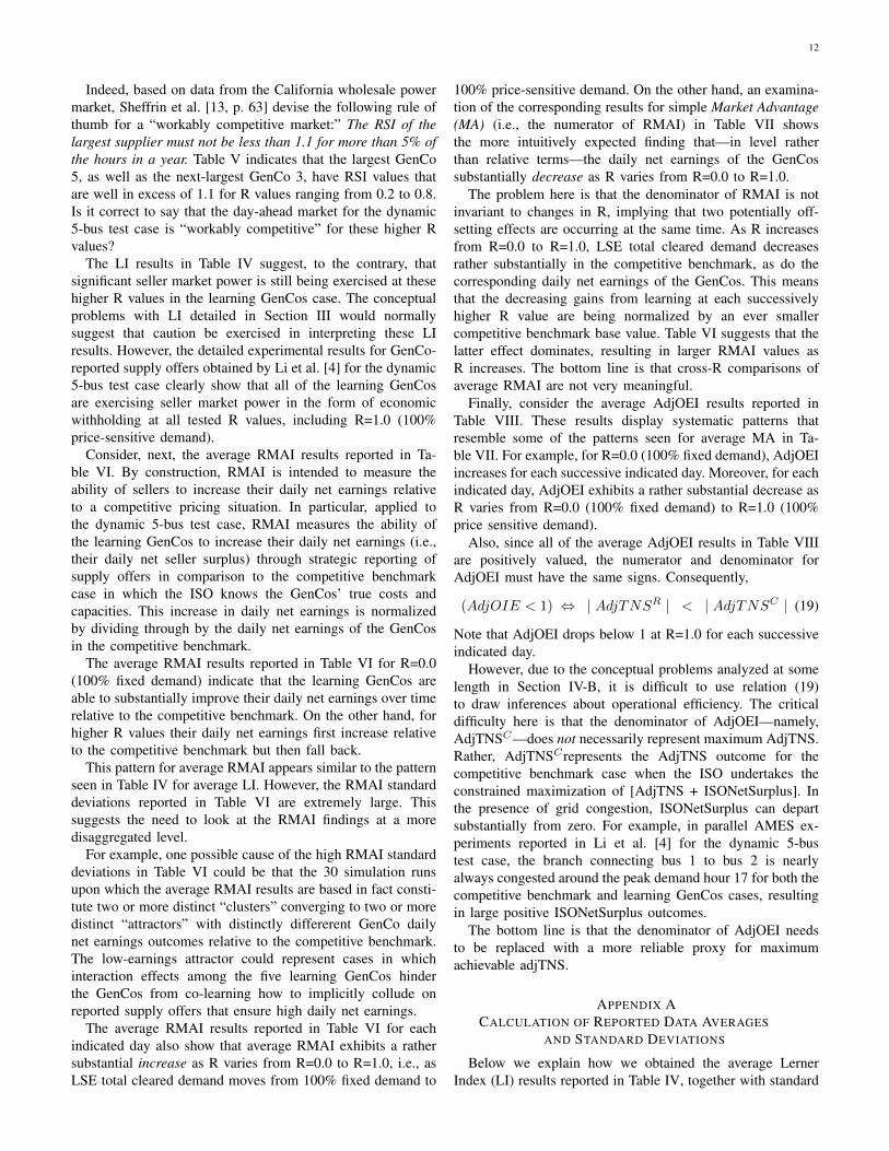
Although relevant for any market, the concept of a pivotalsupplier has special salience for restructured wholesale powermarkets for which much of the bid-in demand is fixed, i.e., notsensitive to price.8 More precisely, electric power effectivelycannot be stored, and imbalances between demand and supplyof electric power on a grid lead to voltage instabilities andultimate grid collapse if not swiftly corrected. For thesereasons, ISOs in wholesale power markets must ensure at alltimes that generation capacity is sufficient to meet total fixeddemand. This requirement means that GenCos in restructuredwholesale power markets who are pivotal suppliers for totalfixed demand have tremendous potential to exercise sellermarket power through the withholding of their capacity.

The following “Residual Supply Index” tests for the pivotal-supplier status of arbitrary groupings of firms participating ina market.

• Residual Supply Index (RSI):Let N denote the collection of all firms participating ina market during some time period T. For any subset Sof N , let TotalCap(S) denote the total operating capacityof the firms in S during T. Also, let TotalDemand denotetotal demand during T. Then

RSI(S) =[

TotalCap(N)− TotalCap(S)TotalDemand

](4)

If RSI(S) < 1, the indication is that the firms in S havepotential seller market power because total demand cannotbe met without their capacity. When total demand and firmcapacities are known in advance, the RSI represents an exante measure in the sense that it can be calculated in advanceof actual market outcomes.

The RSI in various forms was first proposed by a group ofresearchers affiliated with the Department of Market Analysisat the California Independent System Operator (CAISO). SeeSheffrin et al. [13, p. 60] for a report on empirical findingsfor these measures applied to CAISO market data. See, also,Mani and Ainspan [17] for applications of RSI to the NewEngland wholesale power market (ISO-NE).

Finally, we present the definition of a market performancemeasure proposed in [8] as a necessary indicator of marketpower for either a buyer or seller. Here we specialize themeasure to a seller.

• Relative Market Advantage Index (RMAI):Let NetEarnC(i) denote the net earnings that a seller iwould earn in competitive equilibrium during some timeperiod T, and let NetEarnA(i) denote the net earningsof seller i in actual market trading during T. AssumingNetEarnC(i) is not zero,

RMAI(i) =[

NetEarnA(i)− NetEarnC(i)NetEarnC(i)

](5)

In order for seller i to have profitably exerted control over themarket price during T, RMAI(i) must necessarily be positively

8For example, in the U.S. Midwest Independent System Operator (MISO),LSEs are permitted to submit demand bids to the ISO for the day-aheadmarket that have both fixed and price-sensitive parts. However, according todemand bid data released by the MISO [9], at the present time only about1% of the total bid-in demand for the day-ahead market is price sensitive.

valued. Consequently, RMAI(i) > 0 is a necessary conditionfor seller i to have exercised seller market power during T.

B. Market Efficiency Measure

Recall from Subsection III-B that market efficiency is saidto hold for a market if maximum extraction of total netsurplus (TNS) is achieved. Moreover, for standard marketcontexts such as depicted in Fig. 7, maximum TNS extractionis achieved in any competitive equilibrium.

Let M denote a standard market context in some timeperiod T. Let TNSC denote the (maximum) TNS that could beextracted in market M in period T in competitive equilibrium,and let TNSA denote the TNS actually extracted in market Mduring T. Assuming TNSC is positively valued, an “Opera-tional Efficiency Index” can be defined for market M duringT as follows:

• Operational Efficiency Index (OEI):

OEI =TNSA

TNSC(6)

If buyers never purchase goods above their maximum willing-ness to pay and sellers never sell goods below their minimumacceptable sale price, OEI ranges between 0 and 1 in valuewith OEI=1 corresponding to 100% market efficiency.

For later purposes, we now specialize the definitions ofnet buyer surplus, net seller surplus, total net surplus, andOEI to markets for electric power. In particular, we considerthe case of J LSEs and I GenCos participating in an ISO-managed day-ahead wholesale power market operating underLMP pricing.

In standard economic terminology, an LSE that has apositive fixed (price-insensitive) demand for electric powerhas a vertical demand curve for these quantity units, implyingan infinite maximum willingness to pay for them. In ISO-managed day-ahead markets, fixed demand must be met inall normal market circumstances. Consequently, this infinitebenefit does not help to distinguish between the efficiencyattained under different (normal) market scenarios because ineffect it cancels out when the benefits arising under any twoof these scenarios are differenced.

For this reason, power economists routinely omit consid-eration of LSE fixed demand benefits in the constructionof measures designed to evaluate relative market efficiency.A special case of this is when all LSE demand is fixedand attention is focused solely on minimization of the totalvariable costs incurred in satisfying this fixed demand. Herewe consider the more general case, reflective of many actualISO-managed day-ahead wholesale power markets, in whichLSE demand bids consist of both fixed and price-sensitiveparts.

Consider an LSE j located at a transmission grid bus k(j)in some day D. Let pS

Lj and pFLj denote the quantities of

electric power that LSE j is cleared to buy in the day-aheadmarket for hour H of day D+1 corresponding to its price-sensitive demand-bid function Dj(p) and its fixed demand bid,respectively. LSE j’s total cleared demand is thus given by

pLj =[pS

Lj + pFLj

](7)

8

Also, let LMPk(j) denote the LMP for bus k(j) in hour H ofday D+1. LMPk(j) is the price that LSE j is committed to payfor each MW of its total cleared demand (7).

The net buyer surplus of LSE j corresponding to its totalcleared demand (7), adjusted to omit the infinitely-valuedbenefit corresponding to its fixed demand, takes the followingform:

AdjNBSLj =∫ pS

Lj

0

[Dj(p)] dp− LMPk(j) · pLj (8)

In (8), Dj(p) denotes LSE j’s maximum willingness to payfor an increment dp of power, evaluated at the power level p.Consequently, the integral term measures the benefit gained byLSE j from the price-sensitive portion pS

Lj of its total cleareddemand pLj , whereas the far-right term denotes the cost toLSE j for its total cleared demand pLj .

Next consider a GenCo i located at a transmission grid busk(i) in some day D. Let pGi denote the quantity of electricpower that GenCo i is cleared to sell in the day-ahead marketfor hour H of day D+1. Also, let LMPk(i) denote the LMPfor bus k(i) in hour H of day D+1. LMPk(i) is the price thatGenCo i is committed to accept in payment for each MW ofits cleared supply pGi.

The net seller surplus of GenCo i corresponding to itscleared supply pGi is therefore given by

NSSGi = LMPk(i) · pGi −∫ pGi

0

[MCi(p)] dp (9)

In (9), MCi(p) denotes GenCo i’s true left-hand marginal cost(minimum acceptable sale price) for an increment dp of power,evaluated at the power level p. Consequently, the integralterm measures the true variable cost incurred by GenCo i forits cleared supply pGi, whereas LMPk(i) · pGi measures thepayments received by GenCo i for this cleared supply.

The total net surplus attained in the day-ahead market inhour H of day D+1, adjusted by omission of the infinite benefitcorresponding to LSE fixed demand, thus takes the followingform:

AdjTNS =J∑

j=1

AdjNBSLj +I∑

i=1

NSSGi (10)

We consider two different calculations of AdjTNS:• AdjTNSC : AdjTNS calculated under competitive bench-

mark conditions in which the ISO knows the true struc-tural attributes of all LSEs and GenCos;

• AdjTNSR: AdjTNS calculated under auction conditionsin which the ISO must depend on the reported demandbids and supply offers of potentially strategic LSEs and/orGenCos with learning capabilities.

In parallel with (6), we then define an “adjusted” operationalefficiency index as follows:

AdjOEI =AdjTNSR

AdjTNSC(11)

The Adjusted OEI (11) does not have as straightforward aninterpretation as the standardly defined OEI (6). For example,AdjTNS calculated under either competitive or auction condi-tions can be negatively valued in the presence of LSE fixed

demands since LSE fixed demand payments are included butLSE fixed demand benefits are not. Moreover, as elaborated inthe following section, the standardly assumed ISO objectivefunction for the day-ahead market does not guarantee thatAdjTNSC equals maximum possible AdjTNS. These issueswill be further addressed in Section VI, where we presentexperimental findings for AdjOEI.

C. ISO Objective Function and Market Efficiency

Economists typically assume that an appropriate marketobjective for policy makers is market efficiency interpretedto mean the maximization of the sum of net buyer and sellersurplus, i.e., total net surplus (TNS). As depicted in Fig. 7,TNS in standard market contexts can be expressed as thearea between the market demand curve and the market supplycurve, and maximum TNS is achieved where these curvesintersect.

The basic objective typically assumed for ISOs in day-ahead markets is the constrained maximization of the area be-tween the market price-sensitive demand curve and the marketsupply curve as constructed from the reported price-sensitivedemand bids and supply offers of the participant traders.9

Many researchers appear to be under the impression that theconstrained maximization of this ISO objective function isequivalent to the constrained maximization of adjusted TNSas constructed in (10) and hence comports well with standardeconomic policy prescriptions for the achievement of marketefficiency. See, for example, Crampton et al. [18, Appendix1.3, pp. 42-44]. However, it will now be shown that this is notnecessarily the case.

Consider, for example, an ISO-managed wholesale powermarket consisting of J LSEs and I GenCos. Let the objectivefunction of the ISO in day D for hour H of the day-aheadmarket in day D+1 be expressed as follows:

BR−CR =J∑

j=1

∫ pSLj

0

[DR

j (p)]dp−

I∑i=1

∫ pGi

0

[MCR

i (p)]dp

(12)In 12, DR

j (p) denotes LSE j’s reported price-sensitive demandfunction, hence the corresponding summed integral expressionBR denotes the reported total benefits to LSEs correspondingto their reported price-sensitive demand bids (i.e., the areaunder their reported price-sensitive demand functions up totheir cleared demands). MCR

i (p) denotes GenCo i’s reportedmarginal cost function, hence the corresponding summedintegral expression CR denotes the reported total variablecosts incurred by GenCos (i.e., the area under their reportedmarginal cost curves up to their cleared supplies).

The question is whether the objective function (12) isequivalent to AdjTNS as constructed in (10). To see why this isnot true in general, consider the following. The payments fromLSEs and to GenCos for the day-ahead market in day D+1 aresettled through the ISO at the end of day D. Let ISONetSurplusdenote the net payments collected by the ISO in the day-D

9Sometimes additional “unit commitment” costs are also included, such asno-load and start-up costs, but this does not affect the essential point of thissection.

9

settlement for hour H of the day-ahead market in day D+1.Using previously introduced terminology, ISONetSurplus canbe expressed as follows: J∑

j=1

LMPk(j) · pLj −I∑

i=1

LMPk(i) · pGi

(13)

Combining (8), (9), (10), (12), and (13), it is seen that

BR − CR =[AdjTNSR + ISONetSurplus

], (14)

where AdjTNSR denotes AdjTNS based on reported demandbids and supply offers.

Clearly the maximization of (14) subject to generationand transmission constraints will not typically ensure themaximization of AdjTNS subject to these same constraints. Itmight be argued that the inclusion of ISO net surplus in (14)along with net buyer and seller surplus is appropriate, sinceISOs are also market participants. However, ISOs are typicallyconstituted as non-profit organizations, meaning they have afiduciary responsibility to oversee energy market operationsfor the securement of social welfare rather than for thesecurement of maximum organizational profits.

Why not simply “correct” the objective function (14) byreplacing it with AdjTNS (or AdjTNSR)? The key difficultyhere is that the LMPs entering into the expression for AdjTNSin (10) are solved for endogenously within the ISO’s opti-mization problem as shadow prices on certain “nodal balanceconstraints” embodying an important physical constraint onpower flow (Kirchhoff’s Current Law). By construction, theseshadow prices measure the marginal cost to the system ofservicing marginal increments of demand at different gridlocations. Any explicit appearance of LMPs as endogenousvariables in the ISO’s optimization problem apart from theirrole as shadow prices on nodal balance constraints would de-stroy their interpretation as shadow prices for these constraintsand hence their valid interpretation as system marginal costs.

Sufficient conditions for equivalence between the con-strained maximization of [AdjTNSR + ISONetSurplus] in (14)and the similarly constrained maximization of AdjTNS in (10)are as follows: (1) LSEs and GenCos report non-strategicdemand bids and supply offers, implying that AdjTNSR =AdjTNS; and (2) grid congestion is absent, implying all LMPscollapse to a single uniform price level. Given condition (2),ISONetSurplus = 0 because the total quantity of electric powersold equals the total quantity of electric power bought.

How likely are these two conditions to hold? With regardto (1), Li et al. ([3], [4]) report AMES experiments indicatingthat strategic profit-seeking GenCos in restructured wholesalepower markets typically have an incentive to report supplyoffers to the ISO that systematically misrepresent their truenet surplus outcomes. This is the case whether or not gridcongestion is present and whether or not the bid-in demandof LSEs is fixed or price sensitive.

With regard to (2), grid congestion is quite common withinrestructured wholesale power markets in the U.S. and increas-ingly in other countries as well. In the presence of grid conges-tion, LMPs can dramatically separate across the grid, hencethe prices paid to the ISO by LSEs can differ substantially

Fig. 8. 5-bus transmission grid for the dynamic 5-bus test case

from the prices received from the ISO by GenCos. Li et al. [4]report consistently positive ISONetSurplus outcomes in a suiteof AMES experiments for a dynamic 5-bus test case in whichgrid congestion persistently arises. It is actually a bit disturbingto realize that maximization of an objective function such as(14) could have the unintended consequence of encouragingthe emergence and persistence of grid congestion.

What can be done, then, to ensure that the constrainedmaximization of [AdjTNSR + ISONetSurplus] at least ap-proximately achieves the similarly-constrained maximizationof AdjTNS? One possible way to help ensure AdjTNSR =AdjTNS would be for an ISO to engage in suitable monitoringof demand bids and supply offers to discourage strategicreporting. Indeed, ISOs in the U.S. now routinely have “marketmonitoring” units for just this purpose.

One possible way to ensure, in effect, that ISONetSur-plus=0 might be for an ISO to institute a policy under whichthe ISONetSurplus (whether positive or negative in sign)is distributed back to participants in “financial transmissionrights” markets as “congestion rent” payments. Alternatively,a positive ISONetSurpus might be used to enhance the wel-fare of market participants through direct ISO investment intransmission or generation. However, neither of these optionsguarantees market efficiency in the original day-ahead market.This issue requires further study.

V. EXPERIMENTAL DESIGN

All market performance experiments reported in this studywere carried out using the AMES test bed [5] developed byH. Li, J. Sun, and L. Tesfatsion. These experiments are basedon a dynamic 5-bus test case characterized by the followingstructural, institutional, and behavioral conditions:• The 5-bus transmission grid configuration is as depicted

in Fig. 8, with transmission grid, LSE, and GenCostructural attributes as presented in Li et al. [4].10

• In particular, the maximum operating capacities of thefive GenCos depicted in Fig. 8 are as follows: 110MW for

10The 5-bus transmission grid depicted in Fig. 8 is due to Lally [19]. Thisgrid configuration is now used extensively in ISO-NE/PJM training manualsto derive quantity and price solutions at a given point in time assuming ISOshave complete and correct information about grid, LSE, and GenCo structuralattributes.

10

Fig. 9. Daily LSE fixed demand (load) profiles for the dynamic 5-bus testcase

GenCo 1 (G1); 100MW for GenCo 2 (G2); 520MW forGenCo 3 (G3); 200MW for GenCo 4 (G4); and 600 MWfor GenCo 5 (G5). Note that the next-to-largest GenCo3 is favorably situated in a potential “load pocket” withrespect to the three LSEs.

• Also, GenCo 4 (the “peaking unit”) has the most costlygeneration. Next in line is GenCo 3. The three remainingGenCos 1, 2, and 5 have more moderate costs.

• The daily fixed demand (load) profiles for the three LSEsare the same from one day to the next. As depicted inFig. 9, each daily fixed demand profile peaks at hour 17.11

• The learning parameters for each of the five GenCos areset at “sweet spot” values shown in Li et al. [4] to bewhere the GenCos as a whole earn the highest averagedaily net earnings.12 The only factor that changes marketoutcomes from one day to the next is GenCo learning.

Since the GenCos rely on stochastic reinforcement learningto determine their supply offers, multiple runs need to beconducted for each experimental treatment to control forpurely random effects. As in Li et al. [4], we conduct thirtyruns for each treatment using thirty distinct random seedsgenerated via the standard Java “random” class.13

Moreover, only one of the five possible stopping rules inAMES(V2.01) was flagged for each experimental run: namely,the stopping rule requiring that each run terminate at a user-designated day DMax. The value set for DMax in each runwas 1000.

The key treatment factor used in our experimental design,originally developed by Li et al. [3], is the ratio R of maximumpotential price-sensitive demand to maximum potential totaldemand. More precisely, for each LSE j and each hour H, let

Rj(H) =SLMaxj(H)MPTDj(H)

. (15)

In (15) the expression SLMaxj(H) denotes LSE j’s maximumpotential price-sensitive demand in hour H as measured bythe upper bound of its purchase capacity interval, and

MPTDj(H) = [pFLj(H) + SLMaxj(H)] (16)

11These profile shapes are adopted from a case study presented in Shahideh-pour et al. [20, p. 296-297].

12In particular, we use the GenCo Case(1,1) learning parameter valuescharacterized by α = 1 and β = 100 in Li et al. [4].

13See Li et al. [4] for these 30 numerical seed values.

Fig. 10. Illustration of the construction of the R ratio for measuring relativedemand-bid price sensitivity for the special case R=0.5

denotes LSE j’s maximum potential total demand in hourH as the sum of its fixed demand pF

Lj(H) and its maximumpotential price-sensitive demand SLMaxj(H) in hour H. Theconstruction of the R ratio is illustrated in Fig. 10.

For our price-sensitive demand experiments we start bysetting all of the R values (15) for each LSE j and eachhour H equal to R=0.0 (the pure fixed-demand case). We thensystematically increase R by tenths, ending with the valueR=1.0 (the pure price-sensitive demand case). A positive Rvalue indicates that the LSEs are able to exercise at least somedegree of price resistance.

The maximum potential price-sensitive hourly demandsSLMaxj(H) for each LSE j are thus systematically increasedacross experiments. However, we control for confoundingeffects arising from changes in overall demand capacity asfollows: For each LSE j and each hour H, the denominatorvalue MPTDj(H) in (16) is held constant across experimentsby appropriate reductions in the fixed demand pF

Lj(H) asSLMaxj(H) is increased. Specifically, MPTDj(H) is set equalacross all experiments to BPF

Lj(H), the hour-H fixed-demandlevel BPF (H) for LSE j specified in Li et al. [4] for theirbenchmark dynamic 5-bus test case. Consequently, for eachtested R value,

pFLj(H) = [1-R] ∗ BPF

Lj(H) ; (17)

SLMaxj(H) = R ∗ BPFLj(H). (18)

Moreover, as R is incrementally increased from R=0.0to R=1.0, we control for confounding effects arising fromchanges in the LSEs’ price-sensitive demand bids by hold-ing fixed the ordinate and slope values {(cj(H),dj(H)):H=00,...,23} for each LSE j. A listing of the specific numericalvalues used can be found in Li et al. [4].

VI. EXPERIMENTAL FINDINGS

This section uses the experimental design outlined in Sec-tion V for the dynamic 5-bus test case to conduct comparativetests of the five market performance measures developed inSection IV.

In particular, we examine outcomes for the Herfindahl-Hirschman Index (HHI) as defined in (1), the Lerner Index (LI)as defined in (3), the Residual Supply Index (RSI) as defined in(4), the Relative Market Advantage Index (RMAI) as definedin (5), and the Adjusted Operational Efficiency Index (AdjOEI)

11

as defined in (11). Average results are reported for R valuesranging from R=0.0 (100% fixed demand) to R=1.0 (100%price-sensitive demand).

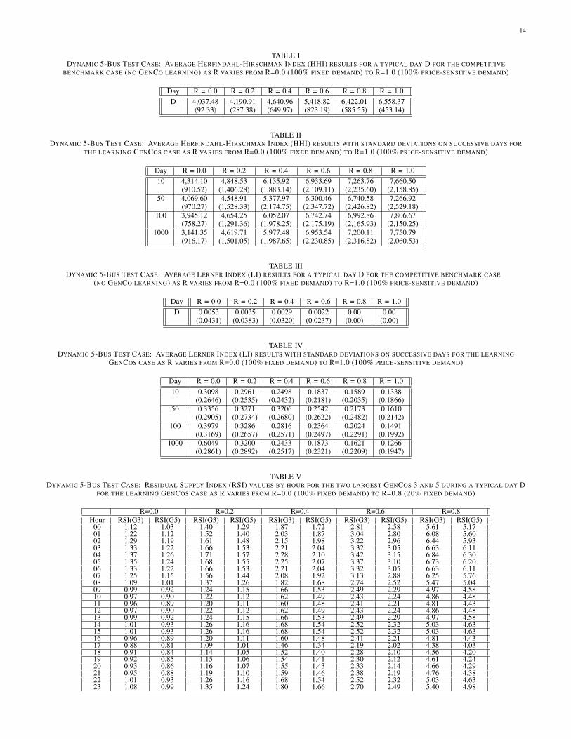
Average HHI and LI results are reported in Tables I throughIV for both the competitive benchmark case (no GenCo learn-ing) and the learning GenCos case. The averages are based on30 runs, each consisting of 1000 time periods (“days”).14 Theonly factor causing changes in market outcomes over time inthe dynamic 5-bus test case is GenCo learning, hence averagesare separately reported for days 10, 50, 100, and 1000 inTables II and IV to check the effects of GenCo learning onHHI and LI valuations over time.

As noted in Section IV-A, larger HHI values indicate ahigher degree of market concentration. Tables I and II showthat, for each tested R value, HHI is generally higher underGenCo learning. Moreover, for each indicated day, HHI sys-tematically increases as R increases. The latter occurs becauseLSE total cleared demand (fixed plus price sensitive) system-atically decreases as R increases, which results in the largerGenCos 3 and 5 supplying a larger share of the decreasingelectric power output. A key question, addressed below, iswhether this higher indicated concentration at higher R valuesin fact indicates a greater exercise of seller market power.

By design, LI is meant to vary directly with seller marketpower. That is, a higher LI value is meant to indicate a greaterexercise of seller market power.

The average LI results reported in Tables III and IV sys-tematically decrease with increases in R for each indicatedday, which suggests that seller market power decreases withincreases in the price sensitivity of LSE demand. The intuitionis that the greater price-sensitivity of demand at higher Rvalues gives LSEs a greater ability to resist higher pricesand hence results in a lowering of average LMP values.This intuition is supported by the LMP experimental findingsreported in Li et al. [4] for the dynamic 5-bus test case;average LMP systematically declines (along with LSE totalcleared demand) as R increases from R=0.0 to R=1.0. Thisdecline is observed both with and without GenCo learning,although average LMP is much higher with GenCo learningthan without for each tested R value.

Comparing these average LI results with the earlier dis-cussed findings for average HHI, it seems fair to say thatHHI is a misleading indicator of seller market power in thecontext of the dynamic 5-bus test case. A similar conclusionis reached by Borenstein et al. [12, Section 4] for othermarket contexts. Conversely, for all of its conceptual faults,the direction of change in average LI correctly indicates thedirection of change in seller market power.

On the other hand, note in Table IV that average LI for thelearning GenCos case systematically increases from day 10 today 1000 for R=0.0 (100% fixed demand), almost doublingby day 1000. However, average LI first increases and thendeclines back approximately to its original level for all positiveR values (i.e., all cases for which LSE total cleared demandis partially price sensitive). This suggests that price sensitivity

14See Appendix A for a more detailed explanation of these average outcomecalculations.

of demand is preventing the learning GenCos from reachingand sustaining the high seller market power levels achievedwith 100% fixed demand.

RSI values are reported in Table V for the two largestGenCos 3 and 5. The “total demand” term in RSI is calculatedto include only LSE fixed demands, hence attention is limitedto R values for which at least a portion of LSE demand isfixed. Since LSE fixed demand profiles and GenCo capacitiesare exogenously given and constant from one day to the next inthe dynamic 5-bus test case, RSI is an ex ante measure whosevalues are also exogenously determined and constant from oneday to the next, independently of whether the GenCos learn ornot. Consequently, it suffices to report RSI values for a typicalday D.

By design, RSI is meant to vary inversely with seller marketpower. That is, a higher RSI value for some GenCo is meantto indicate a smaller potential for the exercise of seller marketpower. Moreover, an RSI value less than 1 for some GenCoindicates a potentially substantial opportunity for this GenCoto exercise seller market power because LSE fixed demandcannot be met without this GenCo’s capacity.

All of the RSI results in Table V follow directly from thedefinition of RSI. In particular, the larger GenCo 5 has a lowerRSI value than the smaller GenCo 3 for each hour and eachtested R value. Moreover, for each hour, each GenCo’s RSIvalue systematically increases with increases in R (i.e., withdecreases in fixed demand), a direct reflection of the increasingease with which the smaller fixed demand can be met fromremaining GenCo capacity. Consequently, the implication fromthese RSI results is that seller market power decreases withincreases in R.

Moreover, RSI systematically dips down for both GenCos ina neighborhood of the peak demand hour 17 for each testedR value, with RSI falling below 1 in this time interval forR=0.0 (100% fixed demand). Consequently, the implication isthat the risk of seller market power is greatest around the peakdemand hour 17, particularly so for the case in which all LSEdemand is fixed.

How do the RSI results reported in Table V compare withthe LI results reported in Tables III and IV? Both sets of resultsindicate that seller market power decreases with increasesin R. Since LI is a direct indicator of seller market powerand RSI is an inverse indicator of seller market power, theseresults support the empirically-based finding of Sheffrin etal. [13, pp. 62-63] that the measures LI and RSI are negativelycorrelated.

Note, however, that RSI exceeds 1 for both GenCos in allhours as soon as R exceeds 0.0, i.e., as soon as a portion ofLSE total cleared demand is price sensitive. An unresolvedissue is the extent to which seller market power can beexercised by GenCos when their RSI values exceed 1.

As recognized by Sheffrin et al. [13], a potential weaknessof the RSI measure (and the pivotal supplier concept moregenerally) is that transmission grid congestion is not taken intoaccount. Consequently, RSI does not reflect the possibility thata load pocket situation can emerge that permits a GenCo toexercise substantial seller market power even though its RSIvalue exceeds 1.

12

Indeed, based on data from the California wholesale powermarket, Sheffrin et al. [13, p. 63] devise the following rule ofthumb for a “workably competitive market:” The RSI of thelargest supplier must not be less than 1.1 for more than 5% ofthe hours in a year. Table V indicates that the largest GenCo5, as well as the next-largest GenCo 3, have RSI values thatare well in excess of 1.1 for R values ranging from 0.2 to 0.8.Is it correct to say that the day-ahead market for the dynamic5-bus test case is “workably competitive” for these higher Rvalues?

The LI results in Table IV suggest, to the contrary, thatsignificant seller market power is still being exercised at thesehigher R values in the learning GenCos case. The conceptualproblems with LI detailed in Section III would normallysuggest that caution be exercised in interpreting these LIresults. However, the detailed experimental results for GenCo-reported supply offers obtained by Li et al. [4] for the dynamic5-bus test case clearly show that all of the learning GenCosare exercising seller market power in the form of economicwithholding at all tested R values, including R=1.0 (100%price-sensitive demand).

Consider, next, the average RMAI results reported in Ta-ble VI. By construction, RMAI is intended to measure theability of sellers to increase their daily net earnings relativeto a competitive pricing situation. In particular, applied tothe dynamic 5-bus test case, RMAI measures the ability ofthe learning GenCos to increase their daily net earnings (i.e.,their daily net seller surplus) through strategic reporting ofsupply offers in comparison to the competitive benchmarkcase in which the ISO knows the GenCos’ true costs andcapacities. This increase in daily net earnings is normalizedby dividing through by the daily net earnings of the GenCosin the competitive benchmark.

The average RMAI results reported in Table VI for R=0.0(100% fixed demand) indicate that the learning GenCos areable to substantially improve their daily net earnings over timerelative to the competitive benchmark. On the other hand, forhigher R values their daily net earnings first increase relativeto the competitive benchmark but then fall back.

This pattern for average RMAI appears similar to the patternseen in Table IV for average LI. However, the RMAI standarddeviations reported in Table VI are extremely large. Thissuggests the need to look at the RMAI findings at a moredisaggregated level.

For example, one possible cause of the high RMAI standarddeviations in Table VI could be that the 30 simulation runsupon which the average RMAI results are based in fact consti-tute two or more distinct “clusters” converging to two or moredistinct “attractors” with distinctly differerent GenCo dailynet earnings outcomes relative to the competitive benchmark.The low-earnings attractor could represent cases in whichinteraction effects among the five learning GenCos hinderthe GenCos from co-learning how to implicitly collude onreported supply offers that ensure high daily net earnings.

The average RMAI results reported in Table VI for eachindicated day also show that average RMAI exhibits a rathersubstantial increase as R varies from R=0.0 to R=1.0, i.e., asLSE total cleared demand moves from 100% fixed demand to

100% price-sensitive demand. On the other hand, an examina-tion of the corresponding results for simple Market Advantage(MA) (i.e., the numerator of RMAI) in Table VII showsthe more intuitively expected finding that—in level ratherthan relative terms—the daily net earnings of the GenCossubstantially decrease as R varies from R=0.0 to R=1.0.

The problem here is that the denominator of RMAI is notinvariant to changes in R, implying that two potentially off-setting effects are occurring at the same time. As R increasesfrom R=0.0 to R=1.0, LSE total cleared demand decreasesrather substantially in the competitive benchmark, as do thecorresponding daily net earnings of the GenCos. This meansthat the decreasing gains from learning at each successivelyhigher R value are being normalized by an ever smallercompetitive benchmark base value. Table VI suggests that thelatter effect dominates, resulting in larger RMAI values asR increases. The bottom line is that cross-R comparisons ofaverage RMAI are not very meaningful.

Finally, consider the average AdjOEI results reported inTable VIII. These results display systematic patterns thatresemble some of the patterns seen for average MA in Ta-ble VII. For example, for R=0.0 (100% fixed demand), AdjOEIincreases for each successive indicated day. Moreover, for eachindicated day, AdjOEI exhibits a rather substantial decrease asR varies from R=0.0 (100% fixed demand) to R=1.0 (100%price sensitive demand).

Also, since all of the average AdjOEI results in Table VIIIare positively valued, the numerator and denominator forAdjOEI must have the same signs. Consequently,

(AdjOIE < 1) ⇔ | AdjTNSR | < | AdjTNSC | (19)

Note that AdjOEI drops below 1 at R=1.0 for each successiveindicated day.

However, due to the conceptual problems analyzed at somelength in Section IV-B, it is difficult to use relation (19)to draw inferences about operational efficiency. The criticaldifficulty here is that the denominator of AdjOEI—namely,AdjTNSC—does not necessarily represent maximum AdjTNS.Rather, AdjTNSCrepresents the AdjTNS outcome for thecompetitive benchmark case when the ISO undertakes theconstrained maximization of [AdjTNS + ISONetSurplus]. Inthe presence of grid congestion, ISONetSurplus can departsubstantially from zero. For example, in parallel AMES ex-periments reported in Li et al. [4] for the dynamic 5-bustest case, the branch connecting bus 1 to bus 2 is nearlyalways congested around the peak demand hour 17 for both thecompetitive benchmark and learning GenCos cases, resultingin large positive ISONetSurplus outcomes.

The bottom line is that the denominator of AdjOEI needsto be replaced with a more reliable proxy for maximumachievable adjTNS.

APPENDIX ACALCULATION OF REPORTED DATA AVERAGES

AND STANDARD DEVIATIONS

Below we explain how we obtained the average LernerIndex (LI) results reported in Table IV, together with standard

13

deviations, for any specified day D and any specified R value.Average and standard deviation calculations for the remainingex post market performance measures are similarly obtained.

First, for each run r, for each hour H (of day D), andfor each GenCo i with a positive cleared power supply pGi

for run r during hour H, determine GenCo i’s Lerner IndexLI(i,r,H,D) as in (3). Second, for each hour H and for eachGenCo i, determine the average of GenCo i’s Lerner IndicesLI(i,r,H,D) across all of the runs r for which GenCo i hada positive cleared power supply for hour H. Third, for eachhour H, determine the average of these run-averaged LernerIndices across all GenCos i that have a positive cleared powersupply during hour H for at least one run r. Finally, determinethe average of these GenCo-averaged and run-averaged LernerIndices across all 24 hours H to get AvgLI(D).

For example, if all of the five GenCos have positive clearedsupplies for each hour H of day D in each run r, AvgLI(D)can be expressed as follows:

AvgLI(D) =

[∑23H=00

∑5i=1

∑30r=1[LI(i, r,H, D)]

]24 ∗ 5 ∗ 30

(20)

The corresponding standard deviation StDevLI(D) is thencalculated using the “N” definition (i.e., division by the totalnumber N=[24*5*30] of summed terms rather than N-1), asfollows:√√√√[∑23

H=00

∑5i=1

∑30r=1[LI(i, r,H, D)−AvgLI(D)]2

]24 ∗ 5 ∗ 30

(21)

ACKNOWLEDGMENT

The authors particularly thank Hongyan Li for many usefuldiscussions related to the topic of this study. We are also grate-ful to Ross Baldick and to Jim McCalley and other membersof our NSF energy project team for helpful comments.

REFERENCES

[1] J. Sun and L. Tesfatsion, “Dynamic testing of wholesale power mar-ket designs: An open-source agent-based framework,” ComputationalEconomics, vol. 30, no. 3, 2007, 291–327. Working paper available:www.econ.iastate.edu/tesfatsi/DynTestAMES.JSLT.pdf

[2] J. Sun and L. Tesfatsion, “DC optimal power flow formulation and so-lution using QuadProgJ,” Proceedings, IEEE Power and Energy SocietyGeneral Meeting, Tampa, Florida, June 2007. Working paper available:www.econ.iastate.edu/tesfatsi/DC-OPF.JSLT.pdf

[3] H. Li, J. Sun, and L. Tesfatsion, “Dynamic LMP response under al-ternative price-cap and price-sensitive demand scenarios,” Proceedings,IEEE Power and Energy Society General Meeting, Pittsburgh, PA, July2008.

[4] H. Li, J. Sun, and L. Tesfatsion, “Separation and volatility of locationalmarginal prices in restructured wholesale power markets,” WorkingPaper (in progress), Economics Department, Iowa State University, 2008.

[5] L. Tesfatsion, AMES Wholesale Power Market Test Bed Homepage,http://www.econ.iastate.edu/tesfatsi/AMESMarketHome.htm

[6] FERC, Notice of White Paper, U.S. Federal Energy Regulatory Com-mission, April 2003.

[7] P. Joskow, “Markets for power in the united states: An interim assess-ment,” The Energy Journal, vol. 27, no. 1, 2006, 1–36.

[8] J. Nicolaisen, V. Petrov, and L. Tesfatsion, “Market power and efficiencyin a computational electricity market with discriminatory double-auctionpricing,” IEEE Transactions on Evolutionary Computation, vol. 5, no. 5,2001, 504–523.

[9] MISO, Homepage, Midwest ISO, Inc., 2008. [Online]. Available:www.midwestiso.org/

[10] ISO-NE, Homepage, ISO New England, Inc., 2008. [Online]. Available:www.iso-ne.com/

[11] R. Baldick and W. Hogan,“Capacity constrained supply function equilib-rium models of electricity markets: Stability, non-decreasing constraints,and function space iterations,” Working Paper Series, Program onWorkable Energy Regulation (POWER), University of California EnergyInstitute, Revised August 2002.

[12] S. Borenstein, J. Bushnell, and C. R. Knittel, “Market power in elec-tricity markets: Beyond concentration measures,” The Energy Journal,vol. 20, no. 4, 1999, 65–88.

[13] A. Y. Sheffrin, J. Chen, and B.F. Hobbs, “Watching watts to preventabuse of power,” IEEE Power and Energy Magazine, July/August, 2004,58–65.

[14] S. Stoft, Power System Economics: Designing Markets for Electricity,Wiley-Interscience, IEEE Press, New York, NY, 2002.

[15] Paul Twomey, Richard Green, Karsten Neuhoff, and David Newbery, “Areview of the monitoring of market power: Possible roles of TSOs inmonitoring for market power issues in congested transmission systems,”05-002 WP, Center for Energy and Environmental Policy Research,March 2005.

[16] L. Pepall, D. J. Richards, and G. Norman, Industrial OrganizationTheory: Contemporary Theory and Practice, South-Western CollegePublishing, Cincinnati, OH, 1999.

[17] S. Mani and A. Ainspan, “Demand response as a tool to alleviate marketpower,” Proceedings, 24th Annual Conference of the USAEE/IAEE, July8-10, Washington, D.C., 2005.

[18] P. Cramton, H.-P. Chao, and R. Wilson, “Review of the proposedreserve markets in New England,” Market Design, Inc., January 2005.www.cramton.umd.edu/papers2005-2009/cramton-chao-wilson-review-of-proposed-reserve-markets.pdf

[19] J. Lally, “Financial transmission rights: Auction example,” in FinancialTransmission Rights Draft 01-10-02, m-06 ed, ISO New England, Inc.,January 2002, section 6.

[20] M. Shahidehpour, H. Yamin, and Z. Li, Market Operations in ElectricPower Systems. New York, NY: IEEE/Wiley-Interscience, John Wiley& Sons, Inc., 2002.

Abhishek Somani is a Ph.D. student in the Department of Economics, IowaState University. His areas of specialization include industrial organization,environmental economics, and computational economics.

Leigh Tesfatsion received her Ph.D. degree in Economics from the Uni-versity of Minnesota in 1975. She is currently Professor of Economics andMathematics at Iowa State University. Her principal research area is Agent-based Computational Economics (ACE), the computational study of economicprocesses modeled as dynamic systems of interacting agents, with a particularfocus on restructured electricity markets. She is an active participant in IEEEPower and Energy Society working groups and task forces focusing on powereconomics issues and serves as associate editor for a number of journals,including the Journal of Energy Markets.

14

TABLE IDYNAMIC 5-BUS TEST CASE: AVERAGE HERFINDAHL-HIRSCHMAN INDEX (HHI) RESULTS FOR A TYPICAL DAY D FOR THE COMPETITIVE

BENCHMARK CASE (NO GENCO LEARNING) AS R VARIES FROM R=0.0 (100% FIXED DEMAND) TO R=1.0 (100% PRICE-SENSITIVE DEMAND)

Day R = 0.0 R = 0.2 R = 0.4 R = 0.6 R = 0.8 R = 1.0D 4,037.48 4,190.91 4,640.96 5,418.82 6,422.01 6,558.37

(92.33) (287.38) (649.97) (823.19) (585.55) (453.14)

TABLE IIDYNAMIC 5-BUS TEST CASE: AVERAGE HERFINDAHL-HIRSCHMAN INDEX (HHI) RESULTS WITH STANDARD DEVIATIONS ON SUCCESSIVE DAYS FOR

THE LEARNING GENCOS CASE AS R VARIES FROM R=0.0 (100% FIXED DEMAND) TO R=1.0 (100% PRICE-SENSITIVE DEMAND)

Day R = 0.0 R = 0.2 R = 0.4 R = 0.6 R = 0.8 R = 1.010 4,314.10 4,848.53 6,135.92 6,933.69 7,263.76 7,660.50

(910.52) (1,406.28) (1,883.14) (2,109.11) (2,235.60) (2,158.85)50 4,069.60 4,548.91 5,377.97 6,300.46 6,740.58 7,266.92

(970.27) (1,528.33) (2,174.75) (2,347.72) (2,426.82) (2,529.18)100 3,945.12 4,654.25 6,052.07 6,742.74 6,992.86 7,806.67

(758.27) (1,291.36) (1,978.25) (2,175.19) (2,165.93) (2,150.25)1000 3,141.35 4,619.71 5,977.48 6,953.54 7,200.11 7,750.79

(916.17) (1,501.05) (1,987.65) (2,230.85) (2,316.82) (2,060.53)

TABLE IIIDYNAMIC 5-BUS TEST CASE: AVERAGE LERNER INDEX (LI) RESULTS FOR A TYPICAL DAY D FOR THE COMPETITIVE BENCHMARK CASE

(NO GENCO LEARNING) AS R VARIES FROM R=0.0 (100% FIXED DEMAND) TO R=1.0 (100% PRICE-SENSITIVE DEMAND)

Day R = 0.0 R = 0.2 R = 0.4 R = 0.6 R = 0.8 R = 1.0D 0.0053 0.0035 0.0029 0.0022 0.00 0.00

(0.0431) (0.0383) (0.0320) (0.0237) (0.00) (0.00)

TABLE IVDYNAMIC 5-BUS TEST CASE: AVERAGE LERNER INDEX (LI) RESULTS WITH STANDARD DEVIATIONS ON SUCCESSIVE DAYS FOR THE LEARNING

GENCOS CASE AS R VARIES FROM R=0.0 (100% FIXED DEMAND) TO R=1.0 (100% PRICE-SENSITIVE DEMAND)

Day R = 0.0 R = 0.2 R = 0.4 R = 0.6 R = 0.8 R = 1.010 0.3098 0.2961 0.2498 0.1837 0.1589 0.1338

(0.2646) (0.2535) (0.2432) (0.2181) (0.2035) (0.1866)50 0.3356 0.3271 0.3206 0.2542 0.2173 0.1610

(0.2905) (0.2734) (0.2680) (0.2622) (0.2482) (0.2142)100 0.3979 0.3286 0.2816 0.2364 0.2024 0.1491

(0.3169) (0.2657) (0.2571) (0.2497) (0.2291) (0.1992)1000 0.6049 0.3200 0.2433 0.1873 0.1621 0.1266

(0.2861) (0.2892) (0.2517) (0.2321) (0.2209) (0.1947)

TABLE VDYNAMIC 5-BUS TEST CASE: RESIDUAL SUPPLY INDEX (RSI) VALUES BY HOUR FOR THE TWO LARGEST GENCOS 3 AND 5 DURING A TYPICAL DAY D

FOR THE LEARNING GENCOS CASE AS R VARIES FROM R=0.0 (100% FIXED DEMAND) TO R=0.8 (20% FIXED DEMAND)

R=0.0 R=0.2 R=0.4 R=0.6 R=0.8Hour RSI(G3) RSI(G5) RSI(G3) RSI(G5) RSI(G3) RSI(G5) RSI(G3) RSI(G5) RSI(G3) RSI(G5)

00 1.12 1.03 1.40 1.29 1.87 1.72 2.81 2.58 5.61 5.1701 1.22 1.12 1.52 1.40 2.03 1.87 3.04 2.80 6.08 5.6002 1.29 1.19 1.61 1.48 2.15 1.98 3.22 2.96 6.44 5.9303 1.33 1.22 1.66 1.53 2.21 2.04 3.32 3.05 6.63 6.1104 1.37 1.26 1.71 1.57 2.28 2.10 3.42 3.15 6.84 6.3005 1.35 1.24 1.68 1.55 2.25 2.07 3.37 3.10 6.73 6.2006 1.33 1.22 1.66 1.53 2.21 2.04 3.32 3.05 6.63 6.1107 1.25 1.15 1.56 1.44 2.08 1.92 3.13 2.88 6.25 5.7608 1.09 1.01 1.37 1.26 1.82 1.68 2.74 2.52 5.47 5.0409 0.99 0.92 1.24 1.15 1.66 1.53 2.49 2.29 4.97 4.5810 0.97 0.90 1.22 1.12 1.62 1.49 2.43 2.24 4.86 4.4811 0.96 0.89 1.20 1.11 1.60 1.48 2.41 2.21 4.81 4.4312 0.97 0.90 1.22 1.12 1.62 1.49 2.43 2.24 4.86 4.4813 0.99 0.92 1.24 1.15 1.66 1.53 2.49 2.29 4.97 4.5814 1.01 0.93 1.26 1.16 1.68 1.54 2.52 2.32 5.03 4.6315 1.01 0.93 1.26 1.16 1.68 1.54 2.52 2.32 5.03 4.6316 0.96 0.89 1.20 1.11 1.60 1.48 2.41 2.21 4.81 4.4317 0.88 0.81 1.09 1.01 1.46 1.34 2.19 2.02 4.38 4.0318 0.91 0.84 1.14 1.05 1.52 1.40 2.28 2.10 4.56 4.2019 0.92 0.85 1.15 1.06 1.54 1.41 2.30 2.12 4.61 4.2420 0.93 0.86 1.16 1.07 1.55 1.43 2.33 2.14 4.66 4.2921 0.95 0.88 1.19 1.10 1.59 1.46 2.38 2.19 4.76 4.3822 1.01 0.93 1.26 1.16 1.68 1.54 2.52 2.32 5.03 4.6323 1.08 0.99 1.35 1.24 1.80 1.66 2.70 2.49 5.40 4.98

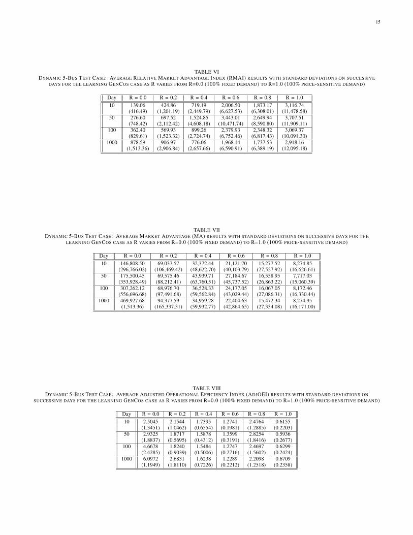
15

TABLE VIDYNAMIC 5-BUS TEST CASE: AVERAGE RELATIVE MARKET ADVANTAGE INDEX (RMAI) RESULTS WITH STANDARD DEVIATIONS ON SUCCESSIVE

DAYS FOR THE LEARNING GENCOS CASE AS R VARIES FROM R=0.0 (100% FIXED DEMAND) TO R=1.0 (100% PRICE-SENSITIVE DEMAND)

Day R = 0.0 R = 0.2 R = 0.4 R = 0.6 R = 0.8 R = 1.010 139.06 424.86 719.19 2,006.50 1,873.17 3,116.74

(416.49) (1,201.19) (2,449.79) (6,627.53) (6,308.01) (11,478.58)50 276.60 697.52 1,524.85 3,443.01 2,649.94 3,707.51

(748.42) (2,112.42) (4,608.18) (10,471.74) (8,590.80) (11,909.11)100 362.40 569.93 899.26 2,379.93 2,348.32 3,069.37

(829.61) (1,523.32) (2,724.74) (6,752.46) (6,817.43) (10,091.30)1000 878.59 906.97 776.06 1,968.14 1,737.53 2,918.16

(1,513.36) (2,906.84) (2,657.66) (6,590.91) (6,389.19) (12,095.18)

TABLE VIIDYNAMIC 5-BUS TEST CASE: AVERAGE MARKET ADVANTAGE (MA) RESULTS WITH STANDARD DEVIATIONS ON SUCCESSIVE DAYS FOR THE

LEARNING GENCOS CASE AS R VARIES FROM R=0.0 (100% FIXED DEMAND) TO R=1.0 (100% PRICE-SENSITIVE DEMAND)

Day R = 0.0 R = 0.2 R = 0.4 R = 0.6 R = 0.8 R = 1.010 146,808.50 69,037.57 32,372.44 21,121.70 15,277.52 8,274.85

(296,766.02) (106,469.42) (48,622.70) (40,103.79) (27,527.92) (16,626.61)50 175,500.45 69,575.46 43,939.71 27,184.67 16,558.95 7,717.03

(353,928.49) (88,212.41) (63,760.51) (45,737.52) (26,863.22) (15,060.39)100 307,262.12 68,976.70 36,528.33 24,177.05 16,067.05 8,172.46

(556,696.68) (97,491.68) (59,562.84) (43,029.44) (27,086.31) (16,330.44)1000 469,927.68 94,377.59 34,959.28 22,404.63 15,472.34 8,274.95

(1,513.36) (165,337.31) (59,932.77) (42,864.65) (27,334.08) (16,171.00)

TABLE VIIIDYNAMIC 5-BUS TEST CASE: AVERAGE ADJUSTED OPERATIONAL EFFICIENCY INDEX (ADJOEI) RESULTS WITH STANDARD DEVIATIONS ON

SUCCESSIVE DAYS FOR THE LEARNING GENCOS CASE AS R VARIES FROM R=0.0 (100% FIXED DEMAND) TO R=1.0 (100% PRICE-SENSITIVE DEMAND)

Day R = 0.0 R = 0.2 R = 0.4 R = 0.6 R = 0.8 R = 1.010 2.5045 2.1544 1.7395 1.2741 2.4764 0.6155

(1.3451) (1.0462) (0.6554) (0.1981) (1.2885) (0.2203)50 2.9325 1.8717 1.5878 1.3599 2.8254 0.5936

(1.8837) (0.5695) (0.4312) (0.3191) (1.8416) (0.2677)100 4.6678 1.8240 1.5484 1.2747 2.4697 0.6299

(2.4285) (0.9039) (0.5006) (0.2716) (1.5602) (0.2424)1000 6.0972 2.6831 1.6238 1.2289 2.2098 0.6709

(1.1949) (1.8110) (0.7226) (0.2212) (1.2518) (0.2358)