HAL Id: hal-02877620https://hal.archives-ouvertes.fr/hal-02877620

Submitted on 22 Jun 2020

HAL is a multi-disciplinary open accessarchive for the deposit and dissemination of sci-entific research documents, whether they are pub-lished or not. The documents may come fromteaching and research institutions in France orabroad, or from public or private research centers.

L’archive ouverte pluridisciplinaire HAL, estdestinée au dépôt et à la diffusion de documentsscientifiques de niveau recherche, publiés ou non,émanant des établissements d’enseignement et derecherche français ou étrangers, des laboratoirespublics ou privés.

AN ADAPTIVE N -FIDELITY METAMODEL FORDESIGN AND OPERATIONAL-UNCERTAINTY

SPACE EXPLORATION OF COMPLEXINDUSTRIAL PROBLEMS

A Serani, R. Pellegrini, R Broglia, J. Wackers, Michel Visonneau, M. Diez

To cite this version:A Serani, R. Pellegrini, R Broglia, J. Wackers, Michel Visonneau, et al.. AN ADAPTIVE N -FIDELITY METAMODEL FOR DESIGN AND OPERATIONAL-UNCERTAINTY SPACE EXPLO-RATION OF COMPLEX INDUSTRIAL PROBLEMS. VIII International Conference on Computa-tional Methods in Marine Engineering MARINE, 2019. �hal-02877620�

VIII International Conference on Computational Methods in Marine EngineeringMARINE 2019

R. Bensow and J. Ringsberg (Eds)

AN ADAPTIVE N-FIDELITY METAMODEL FOR DESIGNAND OPERATIONAL-UNCERTAINTY SPACE

EXPLORATION OF COMPLEX INDUSTRIAL PROBLEMS

A. SERANI∗, R. PELLEGRINI∗, R. BROGLIA∗,J. WACKERS†, M. VISONNEAU†, AND M. DIEZ∗

∗CNR-INM, National Research Council-Institute of Marine EngineeringVia di Vallerano 139, 00128 Rome, Italy

e-mail: {andrea.serani, riccardo.pellegrini}@inm.cnr.it, {riccardo.broglia, matteo.diez}@cnr.it

†LHEEA Lab, Ecole Centrale de Nantes, CNRS-UMR6598, 44321 Nantes Cedex 3, France

e-mail: {jeroen.wackers, michel.visonneau}@ec-nantes.fr

Key words: Multi-fidelity, adaptive metamodels, simulation-based design optimization, uncer-tainty quantification, adaptive-grid refinement, multi-grid acceleration

Abstract. An adaptive N -fidelity (NF) metamodel is presented for the solution of simulation-based design optimization and uncertainty quantification problems. A multi-fidelity approxima-tion is built by an additive correction of a low-fidelity metamodel with metamodels of hierarchicaldifferences (errors) between higher-fidelity levels. The metamodel is based on the expected valueof an ensemble of stochastic radial-basis functions, which also provides the uncertainty associ-ated to the prediction. New training points are added to the appropriate fidelity level, basedon the NF prediction uncertainty and the computational cost. The method is demonstrated foran analytical test function, the shape optimization of a NACA hydrofoil, and the operational-uncertainty quantification of a RoPax ferry. The fidelity levels are defined by adaptive-gridrefinement and multi-grid approach, for the NACA hydrofoil and the RoPax ferry, respectively.The generalization of the multi-fidelity concept to N fidelities shows promising results both interms of accuracy and computational cost.

1 INTRODUCTION

Ship performance depends on design and operational (including environmental) parame-ters. The accurate prediction of significant design metrics (such as resistance and poweringrequirements; seakeeping, maneuverability, and dynamic stability; structural response and fail-ure) requires prime-principle-based high-fidelity computational tools (e.g., for computationalfluid/structural dynamics, CFD/CSD), especially for innovative configurations and off-designconditions. These tools are generally computationally expensive, making the exploration of de-sign (such as in simulation-based design optimization, SBDO) and operational-uncertainty (such

1

Serani A., Pellegrini R., Broglia R., Wackers J., Visonneau M., and Diez M.

as in uncertainty quantification, UQ) spaces a technological challenge.To reduce the computational cost of SBDO and UQ processes, metamodeling methods have

been developed and successfully applied in several engineering fields [1]. Among other meta-models, radial basis functions (RBF) methods have demonstrated their accuracy and efficiencyin engineering design [2]. Further efficiency is gained using dynamic metamodels, for which thedesign of experiments (DoE) for metamodel training is not defined a priori but dynamicallyupdated, exploiting the information that becomes available during the analysis process. Thus,training points are added where it is most useful, reducing the number of function evaluationsrequired to properly represent the function. An adaptive sampling criterion based on the maxi-mum prediction uncertainty for dynamic radial basis functions (DRBF) has been presented by[3]. Other sampling approaches are based on the expected improvement [4] and multi-criteriaadaptive sampling [5].

In addition to dynamic metamodels, multi-fidelity approximation methods have been devel-oped to further reduce the cost of the SBDO procedure, combining the accuracy of high-fidelitysolvers with the computational cost of low-fidelity solvers. Multi-fidelity (MF) metamodels usemainly low-fidelity simulations and few high-fidelity (accurate, expensive) simulations are usedto preserve the accuracy of the overall model. Several metamodels have been used in the litera-ture with MF data, like non-intrusive polynomial chaos [6], co-kriging [7] and RBF [8]. In SBDObased on CFD computations, high- and low-fidelity evaluations may be obtained by varying thephysical model, the size of the computational grid, and/or combining experimental data withnumerical simulations [9]. Most MF approaches generally use two fidelity levels.

The objective of the present work is to formulate and assess an N -fidelity (NF) metamodelfor design and operational-uncertainty space exploration of complex industrial problems.

The NF metamodel is developed as an extension of the authors’ previous work [10]. Themethodology is tested on a 1-D analytical problem and then applied to: (i) the shape optimiza-tion of a NACA hydrofoil and (ii) the uncertainty quantification of a roll-on/roll-off passengers(RoPax) ferry. CFD computations are based on two unsteady Reynolds averaged Navier-Stokesequations (RANSE) solvers: (1) ISIS-CFD [11], developed at Ecole Centrale de Nantes/CNRSand integrated in the FINE/Marine simulation suite from NUMECA Int, for the SBDO problem;(2) χnavis [12], developed at CNR-INM, for the UQ problem. In ISIS-CFD, mesh deformationand adaptive grid refinement techniques are adopted to allow the automatic shape deformationof the hydrofoil. The fidelity levels are defined by the grid refinement ratio. In χnavis, differentfidelities are obtained using multi-grids.

2 N-FIDELITY METAMODEL

Consider x ∈ RD as the design and/or operational uncertainty vector of dimension D. Letthe true function f(x) be assessed by MF simulations: the highest-fidelity level is f1(x), thelowest-fidelity is fN (x), and arbitrary intermediate fidelity levels are {fi}N−1

i=2 (x). Let training

sets be available for each level: {Ti}Ni=1 = {xj , fi(xj)}Jij=1, with {Ji}Ni=1 the training set size.Then an intra-level error εi(x) = fi(x) − fi+1(x) can be defined with an associate training setEi = {(x, fi(x)− fi+1(x)) |x ∈ Ti ∩ Ti+1}.

Using these sets, metamodels fN and {εi}N−1i=1 are trained, where “∼” denotes metamodel

prediction based on a stochastic ensemble of radial basis functions, which also provides the

2

Serani A., Pellegrini R., Broglia R., Wackers J., Visonneau M., and Diez M.

prediction uncertainty U . Assuming the uncertainty associated to the prediction of the lowest-fidelity UfN and intra-level errors Uεi as uncorrelated, the NF approximation f(x) of f(x) andits uncertainty Uf reads

f(x) = fN (x) +

N−1∑i=1

εi(x) and Uf (x) =

√√√√U2fN

(x) +

N−1∑i=1

U2εi

(x) (1)

The contribution of each fidelity level to Uf is assessed and used to refine adaptively the training

sets as the sampling of the design/operational space progresses.

2.1 Adaptive sampling method

The NF metamodel is dynamically updated by iteratively adding a new training point fol-lowing a two-step procedure (see Fig. 1): firstly, the coordinates of the new training point x?

are identified based on the metamodel maximum uncertainty [10], solving the single-objectivemaximization problem:

x? = argmaxx

[Uf (x)]. (2)

secondly, once x? is identified, either TN or all the training sets from Tk to Tk+1 are refinedaccording to Eq. 3. Defining βi = ci+1/ci, i = 1, ..., N − 1, where ci is the computational costassociated to the i-th level, U ≡ {β1Uε1 , ..., βN−1UεN−1 , UfN } as the metamodel uncertaintyvector, and k = maxloc(U):{

If k = N add {x?, fN (x?)} to TN ,else, add {x?, fi(x?)} to Ti with i = k, k + 1

(3)

In the first case, only the lowest-fidelity evaluation is performed, whereas two evaluations arerequired at the same x? in the second case.

2.2 Stochastic radial basis functions

The metamodel prediction f (x) is computed as the expected value (EV) over a stochastictuning parameter of the RBF metamodel, τ ∼ unif[1, 3]:

f (x) = EV [g (x, τ)]τ , with g (x, τ) =

J∑j=1

wj ||x− xj ||τ , (4)

where wj are unknown coefficients, ||·|| is the Euclidean norm. The coefficients wj are determinedenforcing exact interpolation at the training points g (xj , τ) = f (xj) by solving Aw = f , withw = {wj}, alj = ||xl − xj ||τ and f = {f (xj)}.

The uncertainty Uf

(x) associated with the stochastic RBF metamodel prediction is quantified

by the 95%-confidence interval of g(x, τ), evaluated using a Monte Carlo sampling over τ [3].

3

Serani A., Pellegrini R., Broglia R., Wackers J., Visonneau M., and Diez M.

Given the initial training sets

Identify the errors

training sets

Compute the error metamodels

Compute the lowest-fidelitymetamodel

Evalute the global

uncertainty

Stopping criterionsatisfied?

End

Identify new

training point

Build the uncertainty

vector U

maxloc(U) = N

Add new sample

Add new sample

Yes

No

Yes

No

Figure 1: N -fidelity adaptive sampling procedure.

3 ANALYTICAL TEST

One analytical test problem is selected to assess the adaptive NF metamodel performance. Itis mono-dimensional and multi-modal. Figure 2a shows the highest-fidelity level (f1), whereasFigs. 2b and c show, respectively, the same analytical function along with one (f2) and two(f2,3) lower-fidelities and the corresponding errors (ε1,2). The analytical test is defined in Tab.1.

−10 −5 0

x [−]

0

10

20

f(x

)

f1

(a) N = 1

−10 −5 0

x [−]

0

10

20

f(x

)

f1

f2

ε1

(b) N = 2

−10 −5 0

x [−]

0

10

20

f(x

)

f1

f2

f3

ε1

ε2

(c) N = 3

Figure 2: Analytical test problem with different number of fidelities N .

4

Serani A., Pellegrini R., Broglia R., Wackers J., Visonneau M., and Diez M.

Table 1: Analytical test problem.

N Problem Domain

1 f1(x) = −0.5x(sin(0.25x) cos(0.5x) + 1− ex + 2.0) + 8 [−12, 2]

2 f1(x) = −0.5x(sin(0.25x) cos(0.5x) + 1− ex + 2.0) + 8[−12, 2]f2(x) = f1(x)− ε1(x)

ε1(x) = 0.075(x)2 + 3 cos(0.5x− 0.76) + 3

3 f1(x) = −0.5x(sin(0.25x) cos(0.5x) + 1− ex + 2.0) + 8

[−12, 2]f2(x) = f1(x)− ε1(x)f3(x) = f2(x)− ε2(x)ε1(x) = 0.075x2

ε2(x) = 3 cos(0.5x− 0.76) + 3

4 NACA HYDROFOIL SHAPE OPTIMIZATION PROBLEM

This problem addresses the drag minimization of a NACA four-digit airfoil. The followingminimization problem is solved

minimize CD(x)subject to CL(x) = 0.6

and to l ≤ x ≤ u(5)

where x is the design variable vector, CD and CL are respectively the drag and lift coefficient,and l and u are the lower and upper bound of x. The equality constraint on the lift coefficientis necessary in order to compare different geometries at the same lift force (typically equal tothe weight of the object), since the drag depends strongly on the lift.

The hydrofoil shape (see Fig. 3) is defined by the general equation for four-digit NACA foils.The upper (yu) and lower (yl) hydrofoil surfaces are computed as

ξu = ξ − yt sin θξl = ξ + yt sin θyu = yc + yt cos θyl = yc − yt cos θ

with yc =

m

p2

[2pξ

c−(ξ

c

)2], 0 ≤ ξ < pc

m

(1− p)2

[(1− 2p) + 2p

ξ

c−(ξ

c

)2], pc ≤ ξ ≤ c

(6)

where ξ is the position along the chord, c the chord length, yc the mean camber line, p thelocation of the maximum camber, m the maximum camber value, and yt the half thickness

0.0 0.2 0.4 0.6 0.8 1.0

x/c [−]

−0.05

0.00

0.05

0.10

0.15

y/c

[−]

NACA 4− digit

camber line

Figure 3: NACA 4-digit hydrofoil.

5

Serani A., Pellegrini R., Broglia R., Wackers J., Visonneau M., and Diez M.

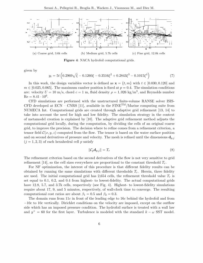
(a) Coarse grid, 3.6k cells (b) Medium grid, 5.7k cells (c) Fine grid, 12.8k cells

Figure 4: NACA hydrofoil computational grids.

given by

yt = 5t(

0.2969√ξ − 0.1260ξ − 0.3516ξ2 + 0.2843ξ3 − 0.1015ξ4

)(7)

In this work, the design variables vector is defined as x = {t,m} with t ∈ [0.030, 0.120] andm ∈ [0.025, 0.065]. The maximum camber position is fixed at p = 0.4. The simulation conditionsare: velocity U = 10 m/s, chord c = 1 m, fluid density ρ = 1, 026 kg/m3, and Reynolds numberRe = 8.41 · 106.

CFD simulations are performed with the unstructured finite-volume RANSE solver ISIS-CFD developed at ECN – CNRS [11], available in the FINETM/Marine computing suite fromNUMECA Int. Computational grids are created through adaptive grid refinement [13, 14] totake into account the need for high and low fidelity. The simulation strategy in the contextof metamodel creation is explained by [10]. The adaptive grid refinement method adjusts thecomputational grid locally, during the computation, by dividing the cells of an original coarsegrid, to improve the precision. The decision where to refine comes from a refinement criterion, atensor field C(x, y, z) computed from the flow. The tensor is based on the water surface positionand on second derivatives of pressure and velocity. The mesh is refined until the dimensions dp,j(j = 1, 2, 3) of each hexahedral cell p satisfy

‖Cpdp,j‖ = Tr (8)

The refinement criterion based on the second derivatives of the flow is not very sensitive to gridrefinement [14], so the cell sizes everywhere are proportional to the constant threshold Tr.

For NF optimization, the interest of this procedure is that different fidelity results can beobtained by running the same simulations with different thresholds Tr. Herein, three fidelityare used. The initial computational grid has 2,654 cells, the refinement threshold value Tr isset equal to 0.1, 0.2, and 0.4 from highest- to lowest-fidelity. The actual computational gridshave 12.8, 5.7, and 3.7k cells, respectively (see Fig. 4). Highest- to lowest-fidelity simulationsrequire about 17, 9, and 5 minutes, respectively, of wall-clock time to converge. The resultingcomputational cost ratios are about β1 = 0.5 and β2 = 0.3.

The domain runs from 11c in front of the leading edge to 16c behind the hydrofoil and from−10c to 10c vertically. Dirichlet conditions on the velocity are imposed, except on the outflowside which has an imposed pressure condition. The hydrofoil surface is treated with a wall lawand y+ = 60 for the first layer. Turbulence is modeled with the standard k − ω SST model.

6

Serani A., Pellegrini R., Broglia R., Wackers J., Visonneau M., and Diez M.

To maintain a constant lift (see Eq. 5), the angle of incidence α for the hydrofoil is adjusteddynamically during the simulations.

The budget is defined in terms of normalized computational cost and is equal to 22. Theinitial training set for the problem is a set of 2N + 1 points including the domain center andmin/max coordinates for each variable. All fidelities are sampled in these points.

5 ROPAX UNCERTAINTY QUANTIFICATION PROBLEM

This problem addresses the UQ of a RoPax ferry in terms of estimation of expected value(EV) and standard deviation (SD) of the (model-scale) resistance (RT ), subject to operationaluncertainty. Specifically, the uncertain parameter is the Froude number with a uniform proba-bility density function from 0.25 to 0.35. The RoPax ferry is characterized by: length betweenperpendicular LPP = 162.85 m, displacement (DWT) of 5, 000 t, block coefficient CB = 0.5677.The analysis is performed with a scale factor λ = 27.14. The parametric geometry of the RoPaxis produced with the computer-aided design (CAD) environment integrated in the CAESES R©

software, developed by FRIENDSHIP SYSTEMS AG, and made available in the framework ofthe H2020 EU Project Holiship.

The hydrodynamics performance of the RoPax is assessed by the unsteady RANSE codeχnavis developed at CNR-INM. It is based on finite volume scheme, with variable co-locatedat cell centers. Turbulent stresses are taken into account by the Boussinesq hypothesis, withSpallart-Almaras turbulence model. Free-surface effects are taken into account by a single-phaselevel-set algorithm. Wall-functions are not adopted, therefore y+ = 1 is ensured on the wall.On solid walls, the velocity is set equal to zero and zero normal gradient is enforced on thepressure field; at the (fictitious) inflow boundary, velocity is set to the undisturbed flow valueand the pressure is extrapolated from the inside; the dynamic pressure is set to zero at theoutflow, whereas the velocity is extrapolated from inner points. On the top boundary, whichremains always in the air region, fluid dynamic quantities are extrapolated from inside. Chimeraoverlapping grid capabilities are used, the numerical solutions are computed by means of a fullmulti grid–full approximation scheme (FMG–FAS), with four grid levels (from coarser to finer:G4, G3, G2, and G1), each obtained from the next finer grid with a refinement ratio equal to2, resulting in β1 = 0.125 and β2 = 0.0625. In the FMG–FAS approximation procedure, the

(a) CFD hull grid (b) Non-dimensional wave elevation, Fr =0.245

Figure 5: RoPax ferry.

7

Serani A., Pellegrini R., Broglia R., Wackers J., Visonneau M., and Diez M.

solution is computed on the coarsest grid level first. Secondly, it is approximated on the nextfiner grid and the solution is iterated by exploiting all the coarser grid levels available with aV-Cycle. The process is repeated up to the finest grid level. For the present UQ problem G1,G2, and G3 grids are used. Simulations are performed considering a water density ρ = 998.2kg/m3, cinematic viscosity ν = 1.105E-6 m2/s, gravitational acceleration g = 9.81 m/s. Thegrid is composed by 53 blocks, for a total of 4.88 M cells, see Fig. 5; the domain extends to2LPP in front of the hull, 3LPP behind, and 1.5LPP each side; a depth of 2LPP is imposed.

6 NUMERICAL RESULTS

The normalized computational cost is defined as 1 for each f1 evaluation and βi, i = 1, ..., N−1for each fi+1 evaluation. It is worth noting that, the normalized computational cost for the CFDproblems is defined, considering only the cost of the highest-fidelity level sampled. This is dueto the fact that, adaptive grid refinement and FMG–FAS compute the solution at grid level kusing solutions from grid level N to k.

The DPSO algorithm presented in [15] is used for the solution of Eqs. 2 and 5.

6.1 Analytical test problem

The performance of the adaptive NF metamodel is assessed in terms of convergence of thenormalized root mean square error (NRMSE), the objective function minimum, and the numberof highest-fidelity evaluations, as shown in Fig.6.

5.0 7.5 10.0 12.5 15.0

Computationl cost [−]

10−1

100

101

102

NR

MS

E%

N = 1

N = 2

N = 3

(a)

5.0 7.5 10.0 12.5 15.0

Computationl cost [−]

7.50

7.75

8.00

8.25

8.50

f min

[−]

N = 1

N = 2

N = 3

(b)

20 40 60 80 100

ANFM iteration [−]

20

40

60

80

100

No.h

igh

est

fid

elit

yev

alu

atio

ns

[−]

N = 1

N = 2

N = 3

(c)

Figure 6: Analytical test problem: convergences of (a) NRMSE, (b) objective function minimum, and(c) the number of the highest-fidelity evaluations versus the sampling procedure iterations.

It is worth noting that for N = 3 the NRMSE decreases faster than for N = 2 and N = 1,achieving an NRMSE = 0.01% with the lowest computational cost (see Fig.6a). Similarly, forN = 3 the minimum of the objective function is achieved with the lowest computational cost (seeFig. 6b). Finally, Fig. 6c shows the number of highest-fidelity evaluations versus the samplingiteration number. It is worth noting that adding intermediate-fidelity levels decreases the needfor highest-fidelity samples.

6.2 NACA hydrofoil shape optimization

Figure 7 shows the training sets at the last iteration of the MF metamodel training for N = 1,2, and 3. For N = 1 the training points are evenly distributed. For N = 2 the low-fidelity

8

Serani A., Pellegrini R., Broglia R., Wackers J., Visonneau M., and Diez M.

2.5

4.5

6.5

m(×

10−

2)

[−]

3.0 7.5 12.0

t(×10−2) [−]

2.5

4.5

6.5

m(×

10−

2)

[−]

3.0 7.5 12.0

t(×10−2) [−]

7.4

7.6

7.8

8.0

8.2

8.4

8.6

CD

[−]

3.0 7.5 12.0

t(×10−2) [−]

5

10

15

20

UCD

%R

Figure 7: NACA hydrofoil: N -fidelity metamodel prediction and associated uncertainty, with N = 1, 2,and 3 from left to right. Black squares, red circles, and green stars are the i = 1, 2, and 3 fidelity trainingsets. Yellow triangles is the minimum position.

evaluations are clustered in three corners. Furthermore, in the latter case the uncertainty of theprediction is significantly higher than for the N = 1 case, suggesting the presence of numericalnoise. Finally, for N = 3 the contour plot of the drag coefficient and the uncertainty looksmoother than for N = 2. This suggests a regularization effect stemming from the use of a mid-level fidelity. At each iteration the predicted minimum is verified through an highest-fidelitysimulation. Fig. 8 shows the convergence of the verified objective function. It is worth notingthat the NF metamodel converges faster for both N = 2 and 3. Table 2 summarizes, the trainingsets size, the normalized cost, the maximum uncertainty of the prediction, the coordinates ofthe predicted minimum of the CD, the predicted minimum, its verification, the prediction error,and the improvement with respect to the original configuration. It is worth noting that for

5 6 7 8 9 10

Normalized cost [−]

7.2

7.4

7.6

7.8

8.0

Op

tim

umCD

(×10−

3)

[−]

N = 1

N = 2

N = 3

Figure 8: NACA hydrofoil: verified optimum convergence versus the normalized computational cost.

9

Serani A., Pellegrini R., Broglia R., Wackers J., Visonneau M., and Diez M.

Table 2: Summary of the adaptive NF metamodel performance on the NACA hydrofoil SBDO problem.

Normalized minimum position minimum value

N |T1| |T2| |T3| cost max(Uf )% t [−] m [−] CD [−] CD [−] E% ∆CD%

1 22 22.0 3.70 6.743E-2 0.000E-2 7.209E-3 7.206E-3 0.1 9.232 8 46 21.8 23.7 5.515E-2 0.000E-2 7.064E-3 7.209E-3 2.0 9.193 5 9 55 20.8 8.78 5.367E-2 0.000E-2 7.094E-3 7.219E-3 1.7 9.07

N = 3 the number of highest-fidelity evaluations decreases compared to N = 1 and 2. Similarimprovements are achieved using N = 1, 2, and 3.

6.3 RoPax uncertainty quantification

The NF metamodel for UQ is assessed through statistical estimation of the expected value(EV) and standard deviation (SD) of the total resistance, RT . The training of the NF metamodelis performed considering at most 4 high-fidelity evaluations. The results are compared to theavailable highest-fidelity CFD data. Figure 9 shows the MF prediction of the total resistanceversus the Froude number, with N =1, 2, and 3. It is worth noting that the increase of Nimproves the MF prediction. Table 3 summarizes the training sets size, the expected value,standard deviation, and associate errors (E) for N = 1, 2, and 3. It is worth noting that theMF metamodel with N = 3 achieves better results than using N = 1 and 2. Furthermore, forN = 3 only three evaluations of the highest-fidelity are performed.

0.250 0.275 0.300 0.325 0.350

Fr [−]

40

50

60

70

RT

[N]

CFD

f (N = 1)

UfT1

0.250 0.275 0.300 0.325 0.350

Fr [−]

40

50

60

70

RT

[N]

CFD

f (N = 2)

Uf

T1

T2

0.250 0.275 0.300 0.325 0.350

Fr [−]

40

50

60

70R

T[N

]CFD

f (N = 3)

Uf

T1

T2

T3

Figure 9: RoPax ferry: model-scale total resistance versus operational uncertainty (Froude number).N = 1, 2, and 3 fidelity metamodels.

Table 3: Summary of the adaptive NF metamodel performance on the RoPax UQ problem.

N |T1| |T2| |T3| Normalized cost EV E(EV)% SD E(SD)%

1 4 4.0000 48.7053 1.8649 1.3904 -38.11792 4 5 4.2500 47.7304 -0.1739 2.1106 -6.06433 3 4 6 3.8125 47.7411 -0.1514 2.1953 -2.2977Reference 9 9 47.8136 - 2.2469 -

10

Serani A., Pellegrini R., Broglia R., Wackers J., Visonneau M., and Diez M.

7 CONCLUSIONS AND FUTURE WORK

The extension of a two-fidelity metamodel [8] to N -fidelity has been presented for the re-duction of the computational cost in solving complex problems by numerical simulations. Themethod has been tested for an analytical test problem, the simulation-based shape-optimizationof a NACA hydrofoil, and the operational-uncertainty quantification of the total resistance of aRoPax ferry at variable advancing speed. The methodology has demonstrated its effectivenessin reducing the computational cost in the problems proposed. For the analytical test problem,the NF method with N = 3 has achieved a greater reduction of the highest-fidelity evaluationsthan with N = 2. For the NACA shape-optimization, the NF method with N = 3 has achievedcomparable solutions to a single-fidelity metamodel, at reduced computational cost. For theoperational-uncertainty quantification, the NF method with N = 3 has achieved better resultsthan with N = 1 and 2, at reduced computational cost. The NACA shape-optimization is likelyaffected by non-negligible numerical noise for the coarser grids. Therefore, future work willaddress the presence of numerical noise [16].

ACKNOWLEDGMENTS

CNR-INM is grateful to Dr. Salahuddin Ahmed and Dr. Woei-Min Lin of the Office of NavalResearch, for their support through NICOP grant N62909-18-1-2033, and to the Italian Ministryof Education for its support through the Italian Flagship Project RITMARE. The HOLISHIPproject (HOLIstic optimisation of SHIP design and operation for life cycle, www.holiship.eu)is also acknowledged, funded by the European Union’s Horizon 2020 research and innovationprogramme under grant agreement N. 689074.

REFERENCES

[1] Viana, F. A. C., Simpson, T. W., Balabanov, V. and Vasilli, T. Special section on mul-tidisciplinary design optimization: Metamodeling in multidisciplinary design optimization:How far have we really come?, AIAA Journal , 52 (4), 670–690, (2014).

[2] Jin, R., Chen, W. and Simpson, T. W. Comparative studies of metamodelling techniquesunder multiple modelling criteria, Structural and Multidisciplinary Optimization, 23 (1),1–13, (2001).

[3] Volpi, S., Diez, M., Gaul, N. J., Song, H., Iemma, U., Choi, K. K., Campana, E. F. andStern, F. Development and validation of a dynamic metamodel based on stochastic radialbasis functions and uncertainty quantification, Structural and Multidisciplinary Optimiza-tion, 51 (2), 347–368, (2015).

[4] Jones, D. R., Schonlau, M. and Welch, W. J. Efficient global optimization of expensiveblack-box functions, Journal of Global Optimization, 13 (4), 455–492, (1998).

[5] Diez, M., Volpi, S., Serani, A., Stern, F. and Campana, E. F., (2019), Simulation-BasedDesign Optimization by Sequential Multi-criterion Adaptive Sampling and Dynamic RadialBasis Functions, pp. 213–228. Springer International Publishing.

11

Serani A., Pellegrini R., Broglia R., Wackers J., Visonneau M., and Diez M.

[6] Ng, L. W.-T. and Eldred, M. Multifidelity uncertainty quantification using non-intrusivepolynomial chaos and stochastic collocation, 53rd AIAA/ASME/ASCE/AHS/ASC Struc-tures, Structural Dynamics and Materials Conference, Structures, Structural Dynamics,and Materials and Co-located Conferences, (2012).

[7] Baar, J. d., Roberts, S., Dwight, R. and Mallol, B. Uncertainty quantification for a sailingyacht hull, using multi-fidelity kriging, Computers & Fluids, 123, 185 – 201, (2015).

[8] Pellegrini, R., Iemma, U., Leotardi, C., Campana, E. F. and Diez, M. Multi-fidelity adaptiveglobal metamodel of expensive computer simulations, 2016 IEEE Congress on EvolutionaryComputation (CEC), July, pp. 4444–4451, (2016).

[9] Kuya, Y., Takeda, K., Zhang, X. and Forrester, A. I. J. Multifidelity surrogate modeling ofexperimental and computational aerodynamic data sets, AIAA Journal , 49 (2), 289–298,(2011).

[10] Pellegrini, R., Serani, A., Diez, M., Wackers, J., Queutey, P. and Visonneau, M. Adap-tive sampling criteria for multi-fidelity metamodels in CFD-based shape optimization, 7thEuropean Conference on Computational Fluid Dynamics (ECFD 7), Glasgow, UK, 11-15June, (2018).

[11] Queutey, P. and Visonneau, M. An interface capturing method for free-surface hydrody-namic flows, Computers & Fluids, 36 (9), 1481–1510, (2007).

[12] Broglia, R. and Durante, D. Accurate prediction of complex free surface flow around ahigh speed craft using a single-phase level set method, Computational Mechanics, 62 (3),421–437, (2018).

[13] Wackers, J., Deng, G., Guilmineau, E., Leroyer, A., Queutey, P. and Visonneau, M. Com-bined refinement criteria for anisotropic grid refinement in free-surface flow simulation,Computers and Fluids, 92, 209 – 222, (2014).

[14] Wackers, J., Deng, G., Guilmineau, E., Leroyer, A., Queutey, P., Visonneau, M., Palmieri,A. and Liverani, A. Can adaptive grid refinement produce grid-independent solutions forincompressible flows?, Journal of Computational Physics, 344, 364 – 380, (2017).

[15] Serani, A., Leotardi, C., Iemma, U., Campana, E. F., Fasano, G. and Diez, M. Parameterselection in synchronous and asynchronous deterministic particle swarm optimization forship hydrodynamics problems, Applied Soft Computing , 49, 313 – 334, (2016).

[16] Wackers, J., Pellegrini, R., Serani, A., Diez, M. and Visonneau, M. Adaptive multifidelityshape optimization based on noisy cfd data, To be presented at 2019 International Confer-ence on Adaptive Modeling and Simulation (ADMOS 2019), El Campello (Alicante), Spain,27-29 May.

12