An Adaptive Mechanism for Full Coverage in Wireless Sensor Networks

Tzu-Ting Wu Kuo-Feng Ssu

Department of Electrical EngineeringNational Cheng Kung University

Tainan, Taiwan 701

Abstract

The coverage issue in wireless sensor networkshas already attracted numerous researchers. In or-der to lift the utility rate of sensors, it is importantto lessen the number of active sensors that performtasks. This paper describes a decentralized and self-configured mechanism for determining active nodes forthe complete coverage in various system environments.The adaptive mechanism examines the existence ofblind/overlapped area and activates/deactivates ap-propriate sensor nodes. The mechanism can furtherbe extended to location-free environment. Three otherapproaches, OTTAWA, PEAS, and OGDC, were alsoimplemented for performance comparisons. The sim-ulations measured the metrics in Tx/Rx control over-head, energy consumption, size of the active node set,and sensing coverage of the active node set. The re-sults show that the adaptive mechanism aids profits innetwork scalability, energy efficiency, and number ofactive sensor nodes.

Keywords: Wireless sensor networks, coverage, den-sity control, energy efficiency, redundancy elimination.

1 Introduction

Recently, wireless sensor networking (WSN) inte-grates environment sensing and data processing usinglow-cost, low-power and small-sized sensors. Withoutany pre-existing infrastructure or planned deployment,numerous sensors autonomously organize themselvesinto a large-scale sensor network to fulfill complextasks [1–5]. Since WSN is a highly density networkand the sensor nodes may be spread in an arbitrary man-ner, coverage problem thus becomes one of the fun-damental issues. The high density environment maybring both serious collision and overhearing problemthat can exhaust energy rapidly. The coverage mecha-

nism aims at keeping full system coverage ratio withoutthe unnecessary overhearing or the channel monitoringcost. Previous research can be roughly divided into twopatterns: (1) finding the minimum links among all sen-sor nodes to connect the networks [6–12]; (2) searchingfor the minimum set of sensors that can satisfy the sys-tem sensing coverage requirements [13–17]. To keepthe original system coverage ratio, the former pattern,also called topology controlling technology, usuallywould involve the power adjustment rather than turn-ing off redundant nodes. The power adjustment candecrease the connectivity degree and thus ease the over-hearing problem. Several approaches using the latterpattern provide solutions for the environment whereeach sensor’s location information is available. Thesize of active node set and the size of blind area aretwo main factors for the latter pattern. The smallersize of active node set may decrease the sensing ratiodue to some uncovered sensing area. The larger onemay suffer heavy idle listening or collision problems.Therefore, it is important to determine a proper set ofactive sensor nodes. Having a proper active node setnot only provides more efficient spatial reuse of thespectrum utilization but also increases the network ca-pacity. Previous solutions for selecting a set of activesensor node have three main categories, Voronoi-basedsolution [18–21], Bottom-up solution [13, 15, 16], andTop-down solution [14]. Although the first categorysometimes may lead in heavy traffic during buildingthe Voronoi diagram, it can acquire the smaller set ofactive sensor nodes by eliminating redundant sensornodes without the blind area. The bottom-up solutionstarts with the empty active node set. Each sensor nodeexams itself to decide whether to join the active nodeset or not. With location information, this categoryoften achieves light control overhead and a small setof the active node set. In high density wireless sensornetwork environment, the reliability of wireless com-munications may be decreased due to packet collisionsand difficult environments so the bottom-up solutionsmay result in redundant nodes. With the top-down so-

lution, all sensor nodes are in the active node set inthe beginning. The sensors then check whether theyshould be removed from the set. The category cansurely preserve the original coverage but it needs sig-nificant control overhead and a big size of active nodeset.

An adaptive full coverage mechanism with both thebottom-up and top-down features is developed in thepaper. The mechanism aims at not only determininga smaller set of active node set without any blind areabut also exploring the redundant node problem thatmay be caused by unreliable transmissions. The algo-rithm starts as the bottom-up way that enables inactivesensor nodes to join the active node set and activatesactive sensor nodes to eliminate the redundant nodedue to the collision. Using the enhanced adaptive fullcoverage algorithm, an inactive sensor node is capableof detecting the blind spot. A redundant node can alsobe determined by an active node executing the samealgorithm. Moreover, the extension of the location-free environment is introduced. The algorithm locallyexchanges one-hop active neighbor information so thenumber of control packets is limited. The algorithm isalso suitable for high-density networks.

The algorithm has been evaluated using the networksimulator ns-2. Three other node-selecting policies,PEAS, OGDC, and OTTAWA, were also implementedfor performance comparisons. PEAS is a coveragealgorithm for location-free environments. OGDC issimulated as a near optimal solution of the bottom-upsolution. The last one stands for top-down solution.The simulation results show that our algorithm out-performed PEAS in both the coverage and networkscalability. Comparing to OTTAWA, our algorithmhad the better detection ability for redundant activenodes. Moreover, the number of active nodes in ourmechanism was close to the number of active nodes inOGDC.

2 Related works

2.1 Top-down solutions

Some research solve the coverage problem in a top-down way. Each sensor node is in the active node set atthe initiate state and exchanges its location informationwith each other. The solutions try to find out everyredundant node and cut it from the active node set. Anode is a redundant node when its sensing area hasbeen covered by the union of its neighbors’ sensingarea. Li er. al proposed a Voronoi-based algorithmthat can precisely detect every redundant node [19].However, it is difficult to built a Voronoi diagram forthe solution. Tian and Georganas studied this problemin more efficient way that does not need the Voronoi

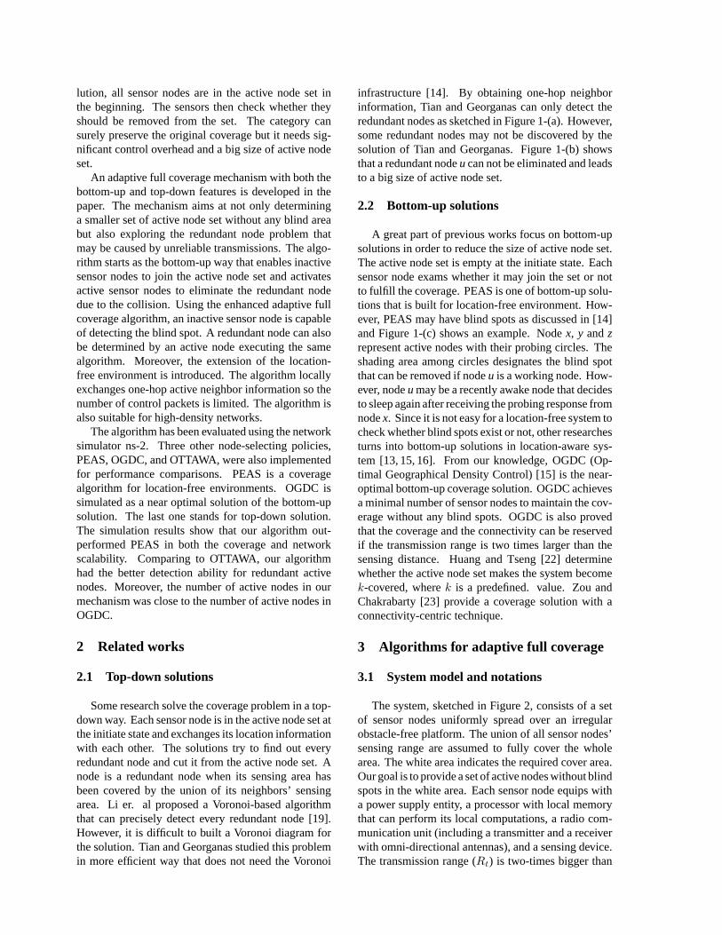
infrastructure [14]. By obtaining one-hop neighborinformation, Tian and Georganas can only detect theredundant nodes as sketched in Figure 1-(a). However,some redundant nodes may not be discovered by thesolution of Tian and Georganas. Figure 1-(b) showsthat a redundant nodeucan not be eliminated and leadsto a big size of active node set.

2.2 Bottom-up solutions

A great part of previous works focus on bottom-upsolutions in order to reduce the size of active node set.The active node set is empty at the initiate state. Eachsensor node exams whether it may join the set or notto fulfill the coverage. PEAS is one of bottom-up solu-tions that is built for location-free environment. How-ever, PEAS may have blind spots as discussed in [14]and Figure 1-(c) shows an example. Nodex, y andzrepresent active nodes with their probing circles. Theshading area among circles designates the blind spotthat can be removed if nodeu is a working node. How-ever, nodeu may be a recently awake node that decidesto sleep again after receiving the probing response fromnodex. Since it is not easy for a location-free system tocheck whether blind spots exist or not, other researchesturns into bottom-up solutions in location-aware sys-tem [13, 15, 16]. From our knowledge, OGDC (Op-timal Geographical Density Control) [15] is the near-optimal bottom-up coverage solution. OGDC achievesa minimal number of sensor nodes to maintain the cov-erage without any blind spots. OGDC is also provedthat the coverage and the connectivity can be reservedif the transmission range is two times larger than thesensing distance. Huang and Tseng [22] determinewhether the active node set makes the system becomek-covered, wherek is a predefined. value. Zou andChakrabarty [23] provide a coverage solution with aconnectivity-centric technique.

3 Algorithms for adaptive full coverage

3.1 System model and notations

The system, sketched in Figure 2, consists of a setof sensor nodes uniformly spread over an irregularobstacle-free platform. The union of all sensor nodes’sensing range are assumed to fully cover the wholearea. The white area indicates the required cover area.Our goal is to provide a set of active nodes without blindspots in the white area. Each sensor node equips witha power supply entity, a processor with local memorythat can perform its local computations, a radio com-munication unit (including a transmitter and a receiverwith omni-directional antennas), and a sensing device.The transmission range (Rt) is two-times bigger than

Figure 1. A sketch of redundant node and blind spot problem.

Figure 2. A sample of two-dimensionalobstacle-free platform.

the sensing range (Rs). In addition to sending and re-ceiving messages, the radio communication providesthe radio signal strength. With the signal strength ofreceived messages, each sensor node can measure thedistance to the sender, based on the following equa-tion [24].

Pr(d) =PtGtGr(ht)2(hr)2

d4L(1)

Several notations are defined for description conve-nience. Sensor nodes that named in capital letter arealways in active node set. Otherwise, the state is notspecified.P is a set that contains triangles endpointsare all belongs active node set.SD, SE , andSF arethree subset from active node set.d(x, y) is the Eu-clidean distance betweenx andy.

3.2 Algorithm

The algorithm is divided into four phases: an ac-tive neighbor electing phase, a blind-spot detectingphase, a redundant-node eliminating phase, and a sens-ing/sleeping phase. At the beginning, each node is setto be an inactive state and contend to be active node.The blind-spot detecting phase makes inactive nodes

Figure 3. An example for active neighborelecting period.

detect whether any blind spot is within their sensingranges and activate themselves if necessary. The re-dundant active nodes can be eliminated after the thirdphase is performed. After performing the first threephases, sensor nodes in the active node set keep on do-ing their sensing tasks while others turn into sleepingstate until next round. Each node maintains an ActiveNeighbor Table (ANT) to record active neighboringinformation.

3.2.1 Active neighbor electing phase

All sensor nodes enable a timer with random durationfor broadcasting HELLO messages in the beginning ofthe active neighbor electing phase. In this phase, aninactive sensor nodeu can be an active sensor nodeonly if its timer successfully expires. When the timerexpires, the inactive sensor node becomes active andbroadcasts the HELLO message that contains its IDand location information. Otherwise, it keeps listeningthe HELLO message from other active sensor nodesand refreshes the information in its ANT. The timeris canceled when an inactive sensor node receives aHELLO message sent by the active sensor node whoselocation is within its sensing range.

Table 1. ANTs for sensor node u, A, B, and C

u A B CNeighbor ID (x,y) Neighbor ID (x,y) Neighbor ID (x,y) Neighbor ID (x,y)

A (xa, ya) B (xa, ya) A (xa, ya) A (xb, yb)B (xb, yb) C (xb, yb) C (xc, yc) B (xc, yc)C (xc, yc)

Table 1 shows four different ANTs for senor nodeA, B, C, andu in Figure 3. Figure 3 indicatesA, B,C, and u contend to be an active sensor node att0.NodeA sends its HELLO message att1 when its timerexpires. Three other nodes,B, C, andu, receive thepacket and refresh their ANT.u cancels its timer dueto d(A, u) ≤ Rs. However, nodeB andC realize thatnodeA is not in its sensing range. Timer of nodeB andC then expires att2 andt3 respectively. An initial activenode set{A,B, C} is generated based on the electionphase. As described in previous section, the activenode set may have blind-spots and redundant-nodes.Thus, the blind-spot detecting phase and the redundantelimination phase will be introduced to discover blindspots and optimize the active node set.

3.2.2 Triangular self-test mechanism

The blind-spot detection phase is based on the trian-gular self-test mechanism where triangles is composedby active sensor nodes in a node’s ANT. Suppose ver-tex A, B, andC are three active sensor nodes in ANT.The broken circles represent the sensing range for eachvertices and are assumed to be identical. Figure 4 illus-trates two acute triangles with their circumcenter (O)whereOA = OB = OC. The circumcenterO(x,y)can be calculated by following equation. If the radius(OA) of the triangle’s circumscribed circle is largerthanRs, a blind spot exists and will be detected.

O(x, y) = (c1 − c2

m2 −m1,m1(

c1 − c2

m2 −m1) + c1) (2)

where m1 =xa − xb

yb − ya,m2 =

xa − xc

yc − ya,

c1 =ya + yb

2−m1(

xa + xb

2),

and c2 =ya + yc

2−m2(

xa + xc

2).

The rule works well when it examines the acute tri-angles. Although the rule also can be applied on obtusetriangles, the rule may work incorrectly and thus leadto lift the size of active node set. For example, in Fig-ure 5, the dotted circles represent sensing ranges forsensor nodeA, B, andC. The broken circle represents

Figure 4. Triangular blind-spot detectionfor acute triangles.

4ABC’s circumscribed circle. Since4ABC is an ob-tuse triangle, the circumcenter must be located outsideof 4ABC. The radius of circumscribed circle (Ro)is longer thanRs. However, the sensing area of theactive sensor nodes (A, B, and C) can fully cover thetriangles and4ABC has no blind spot within itself.This misjudgement may happen frequently so the ac-tive node set will contain numerous redundant nodes.Therefore, an extra examination is needed for the ob-tuse triangles. If an obtuse triangle has more than oneedge longer than 2Rs, the blind spot will appear. Oth-erwise, more analysis are required. Assume thatBCis the longest edge of the obtuse triangle4ABC. DandE are the intersections ofBC, circleB, and circleC. Since vertexD or E is the most farthest uncoveredpoint from vertexA, the coverage of4ABC can beguaranteed only if bothAD andAE are smaller and

Figure 5. Incorrect detection for blindspots in obtuse triangles.

equal toRs.

3.2.3 Blind-spot detecting phase

In blind-spot detecting phase, each inactive sensornode uses the triangular self-test mechanism to de-cide whether to join the active node set or not. Forefficiency and correctness of the blind-spot detection,the triangle should be selected meticulously. Figure 7shows the appropriate triangle setP that is selectedby inactive nodeu where verticesA, B, C, D, E,andF represent the part of active sensor nodes inu’sANT. The process starts with finding the triangle basis- 4ABC. The triangle basis has to encircleu. Atriangle can encircleu if ∠AuB + ∠AuC + ∠BuCis equal to2π. Let G is a set of triangle candidatesthat are formed by active sensor neighbors. TheG setcan be refreshed by pruning off the triangle that cannot satisfy∠AuB + ∠AuC + ∠BuC = 2π. ∠AuB,∠BuC, and∠AuC are defined in equation (3)-(5). Wewould like to choose4ABC that is completely cov-ered by vertexA, B, andC ’s sensing range. If such atriangle basis exists, theP then can be expanded. Oth-erwise, the inactive sensor nodeu finds a blind spot inits sensing range and starts to be an active sensor node.

\AuB = π − arccos(AB2+uA

2−uB2

2AB× 1

uB)

− arccos(AB2+uB

2−uA2

2AB× 1

uA) (3)

\BuC = π − arccos(BC2+uB

2−uC2

2BC× 1

uC)

− arccos(BC2+uC

2−uB2

2BC× 1

uB) (4)

\AuC = π − arccos(AC2+uA

2−uC2

2AC× 1

uC)

− arccos(AC2+uC

2−uA2

2AC× 1

uC) (5)

Since the blind spot may still occur within nodeu’s sensing range as shown in Figure 8. A blind spot

Figure 6. Triangular blind-spot detectionin an obtuse triangle.

exists outside of the triangle basis but withinu’s sens-ing range. Thus,P set must be expanded by adding4ADB, 4BEC, and4AFC that is shown in Fig-ure 7 based on each side of triangle basis. SupposethatLAB : aABx + bABy + cAB = 0, LBC : aBCx +bBCy+cBC = 0, andLAC : aACx+bACy+cAC = 0are line equations that form the triangle basis4ABC.Node u can obtain setSD, SE , andSF by separat-ing its active neighbors from ANT with the followingequations. Nodeu then calculates credits for eachnode in each set with the equation (6)-(8) and com-pares the credits within each set. The node with thebiggest credit from new triangle with other two pointsof4ABC that form the nearest side from itself so theP expanded.

SD =

v

∣∣∣∣∣∣∣∣∣∣∣∣

(vA ≤ 2Rs ∨ vB ≤ 2Rs)∧v 6= A ∧ v 6= B ∧ v 6= C∧

((aABxu + bAByu + cAB ≥ 0∧aABxv + bAByv + cAB ≥ 0)∨(aABxu + bAByu + cAB ≤ 0∧aABxv + bAByv + cAB ≤ 0))

SE =

v

∣∣∣∣∣∣∣∣∣∣∣∣

(vB ≤ 2Rs ∨ vC ≤ 2Rs)∧v 6= A ∧ v 6= B ∧ v 6= C∧

((aBCxu + bBCyu + cBC ≥ 0∧aBCxv + bBCyv + cBC ≥ 0)∨(aBCxu + bBCyu + cBC ≤ 0∧aBCxv + bBCyv + cBC ≤ 0))

Figure 7. An example of appropriate tri-angle set P of node u.

SF =

v

∣∣∣∣∣∣∣∣∣∣∣∣

(vA ≤ 2Rs ∨ vC ≤ 2Rs)∧v 6= A ∧ v 6= B ∧ v 6= C∧

((aACxu + bACyu + cAC ≥ 0∧aACxv + bACyv + cAC ≥ 0)∨(aACxu + bACyu + cAC ≤ 0∧aACxv + bACyv + cAC ≤ 0))

CreditD(v) =

8><>:

(vA×vB)vu if v ∈ SD ∧ uv ≤ 2Rs

(vA+vB)vu if v ∈ SD ∧ uv > 2Rs

(6)

CreditE(v) =

8><>:

(vB×vC)vu if v ∈ SD ∧ uv ≤ 2Rs

(vB+vC)vu if v ∈ SE ∧ uv > 2Rs

(7)

CreditF (v) =

8><>:

(vA×vC)vu if v ∈ SD ∧ uv ≤ 2Rs

(vA+vC)vu if v ∈ SD ∧ uv > 2Rs

(8)

Nodeu exams all the triangles inP by using triangularself-test mechanism for detecting the existence of blindspots. A triangle will be deleted fromP if it is fullycovered. Figure 9-(a) shows a blind spot erroneous di-agnosis whereP contains4ABC and4BEC. An unexistent blind spot is detected in4BEC by triangularself-test mechanism, so the nodeu contends to be anactive node. Nodeu looks over other active nodes inSD, SE , andSF for eliminating the erroneous diag-nosis. The goal is to find an active node that can alsocover the uncovered triangle inP . Figure 9-(b) showsan example where nodeE andW are inSD. Since4BEC can not be fully covered by nodeB, E, andC, nodeu finds nodeW in SD that forms4WEB,4WCB, and4WEC. Nodeu looks over the set un-til these three triangles are all fully covered or the setis employ. Finally,P will be an empty set or contain aset of triangles that has blind spots. IfP is not emptyand the distance from nodeu to each triangle endpointis less and equal to two times of sensing range, node

Figure 8. A blind-spot outside of the u’striangle basis.

u contends to be an active node for covering the blindspots. Otherwise, it computes the intersection pointsformed by the sensing range of the triangle endpoints.Since it is no help for nodeu to be an active node whenall endpoints are not in its sensing range, nodeu onlycontends to be active node when it finds an intersectionpoint in its sensing range.

3.2.4 Redundant-node eliminating phase

The redundant-node eliminating phase is performedby active nodes since wireless communication is anunreliable communication environment. An inactivenode with insufficient information caused by packetcollision or jamming of the channel could be possiblybecome an active node. The phase is similar to theblind-spot detection phase. An active node can off-duty when its sensing range has been fully coveredby its active sensor neighbors. The active node thensends SLEEP message to announce its off-duty. Activenodes contending to be inactive nodes reevaluate theeligibility after receiving the SLEEP messages fromother active nodes. Inactive nodes also reevaluate theeligibility rule for blind-spot detection when receivethe SLEEP messages from its active neighbors.

3.3 State transition

As shown in Figure10, each node can be in oneof three states: SLEEP, ACTIVE, and LISTEN. Thespecified rules of each state can be summarized asfollows:

• LISTEN: The LISTEN state is used for con-structing and refreshing ANT by receiving the

Figure 9. Eliminates the case of incorrectdetection.

HELLO or the SLEEP messages and performingblind-spot detection or redundant node elimina-tion. All nodes are in the LISTEN state and asinactive nodes when the network is initially de-ployed. A collecting timerT0 is triggered whena node turns into the LISTEN state. Each sensornodes decides its state withinT0 and turns intodifferent state whenT0 expires. An inactive nodein the LISTEN state performs blind-spot detect-ing phase and contends to be an active node byrunning join timerTj . Active nodes announcetheir existence in the LISTEN state by sendingthe HELLO messages and wait for a blind-spotdetecting durationTb. Active nodes then performthe redundant node eliminating phase to reevalu-ate its state. The redundant node announces itsnew inactive state by running the sleeping timer

Figure 10. State diagram for adaptivemechanism.

Ts and sensing the SLEEP messages. AfterT0 ex-pires, all active nodes turn into the ACTIVE stateand inactive nodes to the SLEEP state. Figure 11describes the algorithm that is executed byu inthe LISTEN state.

• ACTIVE: The active state is used for perform-ing sensing task and communication. A durationtimerT1 is triggered when the active sensor nodeturns into the ACTIVE state. The active nodeturns into the LISTEN state whenT1 expires.

• SLEEP: The SLEEP state is used to save powerfrom overhearing and performing sensing tasks.The inactive sensor node triggers a duration timerT1 when it changes to the SLEEP state. Whenthe T1 expires, the inactive node turns on its ra-dio, turns into LISTEN state and reevaluates itseligibility.

3.4 Algorithm correctness

Theorem. Given an arbitrary triangle4ABC andthe sensing rangeRs for each endpoint, the blind spotin 4ABC can be detected by the triangular self-testmechanism.

Proof. 4ABC is an acute or a right triangle: It istrivial to use the radius of circumscribed circle to checkthe possible blind spot.4ABC is an obtuse triangle:If two edges are greater than2Rs, the blind spot exists.If each side of4ABC is less than2Rs, no blind spotwill exist. Otherwise, only one edge is larger than2Rs.Suppose that the obtuse triangle is shown in Figure 6.AC is the longest edge and B is the endpoint withthe obtuse angle.D and E are the intersections ofAC, circle A, and circleC. AB andBC are less orequal to2Rs so D and E may be two possible blindspot in4ABC. If both the BD and BE are lessor equal toRs, 4ABC are fully covered by its threeendpoints.

Definition:CurrentState ={ACTIVE, INACTIVE}Initiated state:CurrentState = INACTIVE wait for sending HELLOGotoL1Rules:L1:While wait for sending HELLO

GotoL4EndWhileSending HELLOCurrentState = ACTIVE

L2:While waiting for sending SLEEPGotoL3

EndWhileSending SLEEPCurrentState = INACTIVE

L3:If receiving PACKETRefresh ANTCancel sending current sending SLEEPFind properP set from ANT-{u}GotoL7

EndIfL4:If receiving PACKET

Refresh ANTCancel sending current sending HELLOFind properP set from ANTGotoL7

EndIfL5:If CurrentState == INACTIVE

Prepareto sendHELLOGotoL1

ElseIf CurrentState == ACTIVEWhile CurrentState == ACTIVE

GotoL3EndWhile

EndIfL6:If CurrentState == ACTIVE

Prepareto sendSLEEPGotoL2ElseIf CurrentState == INACTIVE

While CurrentState == ACTIVEGotoL4

EndWhileEndIf

L7:For all4ABC ∈ PIf 4ABC ∈ acute triangle

find circumcenter(O) from4ABC

If max{OA, OB, OC} < Rs

P = P − {4ABC}Else

GotoL8EndIf

ElseIf (max{AB, BC, AC}) ≤ 2Rs

Let F be the endpoint which has the biggest angleDerive coordinates orD andE

If (DF ≤ Rs) ∧ (EF ≤ Rs)P = P − {4ABC}

ElseGotoL8

EndIfElse

GotoL8EndIf

EndForIf P = ∅

GoToL5Else

GoToL6EndIf

L8:For all κ ∈ (ANT − {A, B, C})If4ABκ,4ACκ, and4BCκarefullycoveredtriangles

P = P − {4ABC}Exit For

EndIfEndFor

Figure 11. The Triangular self-test algo-rithm executed by u.

Figure 12. An example demonstrates thecorrectness of the adaptive mechanism.

Definition. If each the sensor node is either an activenode or an inactive node that is covered by activenodes, we define the following phrases:(1) Interior: A sensor node is interior if it has at leastfour triangles in itsP set.(2) Exterior: A sensor node is exterior if it is not aninterior node.

Lemma. Given a fully covered original environment,an interior inactive node can detect all blind spotswithin its sensing range by our mechanism.

Proof. Suppose that nodeu is an inactive interior nodeand the4ABC is its triangle basis as shown in Fig-ure 12. The dotted circle represents theRt and theshadow circle represents the sensing range ofu whichis divided into three sectors:SuAB , SuBC , andSuAC .The sectors are defined byu and three other intersec-tion pointsPuA, PuB , andPuC on u’s sensing circle.For simplicity, we first prove that our mechanism candetect all blind spots withinSuBC by contradiction.Assume that a blind spotX exists within the areaSuBC

and can not be detected by our mechanism.L1 is theline which crosses pointC and the intersection point ofcircleA and circleC. L2 is the line that crosses pointB and the intersection point of circleA and circleB.L3 is the datum line foru to select a triangle forSuBC .Sinceu is an interior node andX is undetectable, theP must contains a fully covered triangle4EBC withbaseBC. A fully covered triangle can be only findwithin the area betweenBC andL1 or betweenBCandL2. Such a triangle is selected by our mechanismthat meansE is the only active node that is most closeto L3. If no other inactive sensor nodes are more closeto L3 in u’s communication range, the proposition that

the environment is fully covered is contradicted. Oth-erwise, such an inactive node may become an activenode when the blind spot aroundCuBC is detected.The new active node triggersu performing our mech-anism again so theX can be detected. Similar proofcan apply onSuAB andSuBC .

Theorem. Given a fully covered environment, the ac-tive node set of our mechanism can form a new topologywithout any interior blind spot.

Proof. Since an interior inactive node can detect allblind spots within its sensing range by our mechanism,the interior blind spot can be eliminated by interiorinactive nodes. The inactive node becomes a memberof active node set when it detects the blind spot. Theactive node set can form a new topology without anyinterior blind spot.

3.5 Discussion

3.5.1 Extension of Location-free environment

The triangular self-test mechanism can apply to thelocation-free environment ifRt ≥ 3Rs. By usingthe signal strength of received messages, sensor nodeu can measure the distance to the sensor based onthe Equation 1. Suppose thatu’s coordinates is (0,0).The endpoints’ locations for its triangle basis can becomputed as

(xb, yb) =

8><>:

xb = −BC2+uB2−uC2

2BC,

yb = − sin(arccos( BC2+uC2−uB2

2BC× 1

uB))× uB,

(9)

(xc, yc) =

8><>:

xc = BC2+uC2−uB2

2BC,

yc = − sin(arccos( BC2+uB2−uC2

2BC× 1

uB))× uC,

(10)

(xa, ya) =

8><>:

xa = xb + AB2+BC2−AC2

2BC,

ya = yb − sin(arccos( AB2+BC2−AC2

2BC×AB))× AB.

(11)

Similar endpoints’ coordinates for each triangle inPcan be derived based on the triangle basis’s coordinates,so the triangular method can be performed correctly.

In order to get sufficient neighboring information forderiving the coordinates, the HELLO message must ap-pend to sender’s ANT. Since ANT refreshes frequentlyat the beginning of the LISTEN state, the HELLO mes-sage must re-send after aTd timer to announce the newANT. The extra payload and the packets may increasethe control overhead while the protocol is executed.The evaluation of the control overhead is discussed inthe section 4.

3.5.2 Scalability and network connectivity

The algorithm is decentralized and executed on eachsensor node in the network. By receiving HELLOmessages from active nodes, inactive nodes can au-tonomously detect blind spots and active nodes canconfirm themselves are a redundant node or not. Thealgorithm will be terminated for an inactive node whenthere is no blind spot in theP set or theP set can not befound. Only active sensor nodes can broadcast HELLOmessages so the number of advertising messages arebounded and will not increase with extensions of thenetwork density. Therefor, the proposed algorithm isscalable to the large and dense networks. The con-nectivity for the output topology of our algorithm canbe also ensured. Based on the discussion of networkconnectivity in [15], the network connectivity can beguaranteed ifRt ≥ 2Rs

4 Simulation results

The algorithm was evaluated by network simulator -ns2 [25] with the CMU wireless extension. Three otherwell-known schemes, PEAS [13], OTTAWA [14], andOGDC [15], were also simulated for comparing toour mechanism with and without location information.PEAS stood for the bottom-up scheme that can ob-tain its active node set in location-free environments,but its coverage performance can not be guaranteed.OTTAWA stood for the top-down scheme within thelocation-aware environment and can guarantee the en-vironment coverage. OGDC is a bottom-up schemewithin the location-aware environment which can ac-quire the minimal active node set. A variety of networkdensities (100, 150, 200, 250, and 300 sensor nodes in a50m×50m square space) were simulated. Ten differentenvironment scenarios were generated using uniformdistribution for each network density.

Table 2 shows the parameters in each scheme. InPEAS, timerT was utilized for decreasing the collisionprobability for probing responses and the transmissionrange (Rt) is double of the sensing range (Rs). InOTTAWA, theRt is equal toRs. Parameters in OGDCwere set based on the values as described in [15]. Thelocation-free adaptive mechanism usedRs = 10 m andRt = 30 m. The five timers (T0, T1, Tj , Td andTs)were set to5, 10, 5 × 10−6, 5 × 10−6, and1 × 10−5

seconds, respectively. The parameters for location-aware mechanism are also listed on Table2.

Three criterions were chosen to evaluate the per-formance for each scheme: (1) Control overhead: itmeasures the total number of packets that transmit-ted/received by/from the sensors (Tx/Rx) and the en-ergy consumption for the protocol lifetime. (2) Cov-erage efficiency: it includes the size of active node set

Table 2. Parameter SettingsSchemes Parameter Settings

Transmission Range Sensing Range Timer Duration

PEAS 20 (m) 10 (m) T =200 (µs)OTTAWA 10 (m) 10 (m) -

OGDC 20 (m) 10 (m) Td =10 (µs),Ts =1 (s),Te =200(µs)

Adaptive 30 (m) 10 (m) T0 =3(s),T1 =10(s),Tj =5 (µs),(Location-free) Ts =5 (µs),Td =10 (µs)

Adaptive 20 (m) 10 (m) T0 =3(s),T1 =10(s),Tj =5 (µs),(Location-aware) Ts =5 (µs)

and the coverage percentage which shows the percent-age of area covered by the selected active node set. (3)Environment adaptability: it reveals the adaptability ofeach protocol with various initial environment states.

4.1 Control overhead

Figure 13 indicates the Tx control overhead foreach protocol where OGDCnoB represents the pro-tocol without any border information. The OT-TAWA ps and Adaptiveps curves represent the num-ber of SLEEP packets caused by executing OTTAWAand our location-aware adaptive protocol. Controloverhead growing with the network density decreasesthe protocol scalability due to the bandwidth limi-tation. There is an immediate sharp increase forPEAS due to the PROBE interaction from the wake-up sensors and the active sensors through its entirelifetime. OTTAWA, the Top-down scheme, also hasits Tx control overhead markedly growing with thenetwork density and its HELLO and SLEEP interac-tions. Since the SLEEP intersection control overheadis slowly increased with the extension of the networkdensity, the scalability limitation of the OTTAWA isthe HELLO intersection at the beginning of the initi-ate state. The location-free adaptive mechanism’s Txpackets is steady but double more than the location-aware one because the active nodes send their HELLOmessages twice to provide enough neighboring infor-mation. The reminder curves in Figure 13 were re-mained steady and were magnified in Figure 14. Thenumber of Tx packet for of OGDC equals to its size ofthe active node set. Since OGDCnoB lacks the bound-ary information, many inactive sensor nodes tend to be-come active nodes to cover the intersection points thatare not within the sensing field. The bottom curve is thenumber of transmitted SLEEP packet that triggered bythe redundant nodes caused by the collision problem.The total number of Tx control packets of triangularprotocol which does not need boundary informationlies in between OGDC and OGDCnoB.

Figure 13. Comparison of numbers of Txpackets versus network density underdifferent mechanisms.

Figure 15 and Figure 16 shows the overall Rx con-trol overhead which can reveal the influence of theoverhearing for each protocol. In Figure 15, all curvesare increased when the network density is enlarged.OTTAWA suffers serious overhearing problem due tiexchanging huge active neighboring information so thecurve grows rapidly. The bottom-up schemes, OGDCand PEAS, ease off such influence by collecting smallset of active neighboring information. Although theperformance of PEAS in Tx control overhead is notefficient, PEAS takes vantage of adaptive sleeping toavoid unnecessary idle listening. Therefore, the curveof PEAS is the same with the curve of OGDCnoB andeven better in high density environments. The curve oflocation-free adaptive mechanism is increased rapidlydue toRt = 3Rs. However, the curve of location-aware mechanism is between the curves of PEAS andOGDC. Figure 16 measures the normalized Rx controloverhead in bytes. The location-free adaptive mecha-nism appends by sender’s ANT to the control packets,the size of control packet is bigger than OGDC and

Figure 14. Detail comparison of numbersof Tx packets versus network density un-der OGDC and Adaptive mechanism.

Figure 15. Comparison of numbers of Rxpackets versus network density underdifferent mechanisms.

OTTAWA which only needs the sender’s location in-formation. Since the packet size of three protocols isbigger than PEAS and do not support adaptive sleepmechanism during its protocol execution time. Thenormalized Rx overhead of PEAS lies between the tri-angular and OGDC protocol. The curves for OGDC,OGDC noB, and the location-aware adaptive methodwere steady through various network density. ThePEAS slightly increased with the network density byusing its adaptive sleeping. The normalized Rx over-head seems huge for our location-free mechanism be-cause each payload must add the sender’s entire ANTand the sensors’ transmission range. However, theoverhead did not raise too much energy consumptionsince the energy consumption of receiving a packet ismuch smaller than that of transmitting a packet.

Figure 17 shows the overall energy consumption of

Figure 16. Comparison of normalizedbytes of Rx control overhead versusnetwork density under different mecha-nisms.

Figure 17. Comparison of energy con-sumption for different mechanisms.

idle listening, transmitting, and receiving. The energydispatching rates of battery power drain for these threestates were 660mW, 395mW, and 35mW, respectively.The actual energy consumption depends on the trans-mission time which is related to the size of the packet.Since the consumption of Tx is almost twice of Rx,Figure 17 matches the results to the Figure 13 to 16.

4.2 Coverage efficiency

The most efficient protocol forms the size of activenode set as small as possible but still has high coveragepercentage. Since the performance of our location-freeand location-aware mechanisms are similar in coverageefficiency and environment capability, the simulationonly lists the result of the latter pattern. Figure 18indicates the size of active node set for all protocols.Figure 19 shows the coverage percentage for each ac-

Figure 18. Comparison of active node setsize versus network density under differ-ent mechanisms.

Figure 19. Comparison of coverage per-centage versus sensing field under dif-ferent mechanisms.

tive node set. In Figure 19 and Figure 20, the x-axisrepresents the side length of the selected square area ofthe sensing field and decreases 2.5 (m) for each side ofthe sensing square. In Figure 19, the cover percentagefor PEAS with various network densities can not reach100% through the entire sensing field. Although theperformance of PEAS upgraded when the network den-sity increased, it is still unsatisfied and unstable. Thecoverage performance for OGDC and adaptive mech-anism are picked in Figure 20. OGDC can guaranteed100% coverage within 45×45 squared sensing field.The Triangular can guaranteed within 40×40 squaredsensing field. Even within sensing field (50×50), boththe OGDC and adaptive mechanisms guaranteed thecoverage over 99%. OTTAWA guaranteed 100% cov-erage though entire sensing field due to its top-downalgorithm. Although the cover percentage seems tosurpass any other protocol, its active node set is not

Figure 20. Detail comparison of cover-age percentage versus sensing field un-der OTTAWA, OGDC, and Adaptive mech-anisms.

Figure 21. Comparison of active node setsize versus various IASR under OTTAWA,OGDC, and Adaptive mechanisms.

stable and increases rapidly due to the serious colli-sion and the redundant node problem as discussed insection 2.1. The active node set for triangular is veryclose to OGDC and smaller than OGDCnoB (see Fig-ure 18). PEAS has a small size of the active nodeset and slowly extends with the increase of the net-work density. However, the coverage performance isunsatisfied.

4.3 Environment adaptability

Since the coverage protocol may be used for net-work topology repairing in different environments, thesimulations for environment adaptability assumed thatthe active node set is not empty at each start. The x-axis in Figure 21 represents the Initiated Active SensorRatio (IASR) which is the proportion from the num-

ber of active sensors to the total number of sensors.The y-axis represents the number of the final activenode set after the protocols are executed. The totalnumber of the sensor nodes is 200 and the referenceline (Ref Line) marks the number of initiated activesensor nodes. The performance of OTTAWA is stabledue to its Top-down executing fashion. The size ofactive node set of OGDC increased rapidly with theRef Line and loss its predominance of the protocol.However, our mechanism acquired the smallest activenode set from the 5% to 100% IASR by performing theredundant-node elimination. The curve for triangularkeeps stable when IASR is less than 20% but growsslowly among 25% to 100% IASR because some re-dundant nodes are not eliminated due to the packet lossproblem. Moreover, the size of active node set is stilltwice smaller than OTTAWA and three times smallerthan OGDC within 50% IASR.

5 Conclusion

The adaptive mechanism explored two challengesin the coverage issue. First, the unreliable wirelesscommunication environment may decrease the per-formance of traditional bottom-up coverage protocol.Second, the location information requirement is not al-ways available. The mechanism based on an adaptivetriangular self-test method not only efficiently patchesup blind-spots but also detects the redundant nodes.The adaptive mechanism has four main advantages.First, 100% cover ratio can be guaranteed in the inte-rior sensing field and the total sensing environment canreach over 99%. Second, the mechanism can be easilyextended to the location-free environment with toler-able control overhead. Third, our mechanism is scal-able for high density environments. Last, the mecha-nism can be applied to the blind-spot or the redundant-node detection so the impact of initial environmentalstates can be reduced. The simulations evaluated con-trol overhead, coverage efficiency, and environmentalscalability. Compared to PEAS, our mechanism guar-anteed the coverage with the lower control overhead.The size of the active set generated by our mechanismwas competitive to OGDC that required global loca-tion information and border information for all sensornodes. Our mechanism even performed better than theOGDC when the border information was unavailable.Moreover, the environmental scalability shows that ourprotocol outperformed both OTTAWA and OGDC with100% IASR.

6 Acknowledgment

This research was supported by the National ScienceCouncil (NSC) under contract NSC 93-2213-E-006-

019 and 94-2213-E-006-076.

References

[1] I. F. Akyildiz, W. Su, Y. Sankarasubramaniam,and E. Cayirci, “Wireless Sensor Networks:A Survey,” Elsevier Computer Communication,vol. 38, no. 4, pp. 393–422, March 2002.

[2] I. F. Akyildiz, W. Su, Y. Sankarasubramaniam,and E. Cayirci, “A Survey on Sensor Networks,”IEEE Communications Magazine, vol. 40, no. 8,pp. 102–114, August 2002.

[3] A. Mainwaring, J. Polastre, R. Szeqcayk, andD. Culler, “Wireless Sensor Networks for HabitatMonitoring,” Proceedings of ACM InternationalWorkshop on Wireless Sensor Networks and Ap-plications (WSNA), pp. 88–97, September 2002.

[4] D. Estrin, R. Govindan, J. Heidemann, and S. Ku-mar, “Next Century Challenges: Scalable Co-ordination in Sensor Networks,”Proceedingsof ACM/IEEE International Conference on Mo-bile Computing and Networking (MOBICOM),pp. 263–270, August 1999.

[5] J. M. Kahn, R. H. Katz, and K. S. J. Pister,“Next Century Challenges: Mobile Networkingfor “Smart Dust”,” Proceedings of ACM/IEEEInternational Conference on Mobile Computingand Networking (MOBICOM), pp. 271–278, Au-gust 1999.

[6] L. Hu, “Topology Control for Multihop PacketRadio Networks,”IEEE Transaction on Commu-nications, vol. 41, no. 10, pp. 1474–1481, Octo-ber 1993.

[7] R. Ramanathan and R. Rosales-Hain, “Topol-ogy Control of Multihop Wireless Networks Us-ing Transmit Power Adjustment,”Proceedingsof IEEE Joint Conference of the IEEE Com-puter and Communications Societies (INFO-COM), pp. 404–413, March 2000.

[8] T.-C. Hou and V. O. K. Li, “Transmission RangeControl in Multihop Packet Radio Networks,”IEEE Transaction on Communications, vol. 34,no. 1, pp. 38–44, January 1986.

[9] R. Wattenhofer, L. Li, P. Bahl, and Y.-M. Wang,“Distributed Topology Control for Power Effi-cient Operation in Multihop Wireless Ad HocNetworks,” Proceedings of IEEE Joint Confer-ence of the IEEE Computer and CommunicationsSocieties (INFOCOM), pp. 1388–1397, April2001.

[10] J. Liu and B. Li, “Distributed Topology Controlin Wireless Sensor Networks with AsymmetricLinks,” Proceedings of IEEE Global Telecommu-nications Conference (GLOBECOM), pp. 1257–1262, December 2003.

[11] A. Cerpa and D. Estrin, “ASCENT: AdaptiveSelf-Configuring sEnsor Networks Topologies,”Proceedings of IEEE Joint Conference of theIEEE Computer and Communications Societies(INFOCOM), pp. 1278–1287, June 2002.

[12] M. Cardei and J. Wu, “Energy-Efficient CoverageProblems in Wireless Ad Hoc Sensor Networks,”accepted to appear in Journal of Computer Com-munications on Sensor Networks, 2004.

[13] F. Ye, J. C. G. Zhong, S. Lu, and L. Zhang,“PEAS: A Robust Energy Conserving Protocolfor Long-lived Sensor Networks,”Proceedingsof IEEE International Conference on DistributedComputing Systems (ICDCS), pp. 28–37, May2003.

[14] D. Tian and N. D. Georganas, “A Coverage-preserving Node Scheduling Scheme for LargeWireless Sensor Networks,”Proceedings of ACMInternational Workshop on Wireless Sensor Net-works and Applications (WSNA), pp. 32–41,September 2002.

[15] H. Zhang and J. C. Hou, “Maintaining Sens-ing Coverage and Connectivity in Large SensorNetworks,” Tech. Rep. UIUCDCS-R-2003-2351,Department of Computer Science, University ofIllinois at Urbana-Champaign, June 2003.

[16] X. Wang, G. Xing, Y. Zhang, R. P. C. Lu, andC. Gill, “Integrated Coverage and Connectiv-ity Configuration in Wireless Sensor Networks,”Proceedings of the First ACM Conference on Em-bedded Networked Sensor Systems (SenSys’03).,pp. 28–38, November 2003.

[17] C.-F. Huang and Y.-C. Tseng, “A Survey of Solu-tions to the Coverage Problems in Wireless Sen-sor Networks,”Journal of Internet Technology,vol. 6, no. 1, pp. 1–8, January 2005.

[18] A. Ghosh, “Estimating Coverage Holes and En-hancing Coverage in Mixed Sensor Networks,”Proceedings of the 29th Annul IEEE Interna-tional Conference on Local Computer Networks(LCN’04)., pp. 68–76, November 2004.

[19] X.-Y. Li, P.-J. Wan, and O. Frieder, “Coverage inWireless Ad Hoc Sensor Network,”IEEE Trans-action on Computers, vol. 52, no. 6, pp. 753–763,November 2003.

[20] S. Meguerdichian, F. Koushanfar, M. Potkon-jak, and M. B. Srivastava, “Coverage problemsin Wireless Ad Hoc Sensor Network,”Proceed-ings of IEEE Joint Conference of the IEEEComputer and Communications Societies (INFO-COM)., pp. 1380–1387, April 2001.

[21] S. Meguerdichian, F. Koushanfar, G. Qu, andM. Potkorjak, “Exposure in wireless ad-hoc sen-sor networks,”Proceedings of ACM/IEEE In-ternational Conference on Mobile Computingand Networking (MOBICOM), pp. 139–150, July2001.

[22] C.-F. Huang and Y.-C. Tseng, “The CoverageProblem in a Wireless Sensor Network,”Proceed-ings of the 2nd ACM International Conferenceon Wireless Sensor Networks and Applications(WSNA), pp. 115–121, September 2003.

[23] Y. Zou and K. Chakrabarty, “A DistributedCoverage- and Connectivity-Centric Techniquefor Selecting Active Nodes in Wireless SensorNetworks,” IEEE Transactions on Computers,vol. 54, no. 8, pp. 978–991, August 2005.

[24] T. S. Rappaport,Wireless communications, prin-ciples and practive. Prentice Hall, 1996.

[25] “The Network Simulator - NS-2.” URLhttp://www.isi.edu/nsnam/ns/.