An Active Learning Approach to Hyperspectral Data Classification

IEEE TRANSACTIONS ON GEOSCIENCE AND REMOTE SENSING, VOL. 46, NO. 4, APRIL 2008 1231

An Active Learning Approach to HyperspectralData Classification

Suju Rajan, Joydeep Ghosh, Fellow, IEEE, and Melba M. Crawford, Fellow, IEEE

Abstract—Obtaining training data for land cover classificationusing remotely sensed data is time consuming and expensive es-pecially for relatively inaccessible locations. Therefore, designingclassifiers that use as few labeled data points as possible is highlydesirable. Existing approaches typically make use of small-sampletechniques and semisupervision to deal with the lack of labeleddata. In this paper, we propose an active learning techniquethat efficiently updates existing classifiers by using fewer labeleddata points than semisupervised methods. Further, unlike semi-supervised methods, our proposed technique is well suited forlearning or adapting classifiers when there is substantial changein the spectral signatures between labeled and unlabeled data.Thus, our active learning approach is also useful for classify-ing a series of spatially/temporally related images, wherein thespectral signatures vary across the images. Our interleaved semi-supervised active learning method was tested on both single andspatially/temporally related hyperspectral data sets. We presentempirical results that establish the superior performance of ourproposed approach versus other active learning and semisuper-vised methods.

Index Terms—Active learning, hierarchical classifier, multi-temporal data, semisupervised classifiers, spatially separate data.

I. INTRODUCTION

R ECENT advances in remote sensing technology havemade hyperspectral data with hundreds of narrow con-

tiguous bands more widely available. The hyperspectral datacan therefore reveal subtle differences in the spectral signaturesof land cover classes that appear similar when viewed bymultispectral sensors [1]. If successfully exploited, the hyper-spectral data can yield higher classification accuracies and moredetailed class taxonomies. However, the task of classifyinghyperspectral data also has unique challenges.

Supervised statistical methods require labeled training datato estimate parameters. It is expensive and time consuming toobtain labeled data, but the very high dimensionality of thehyperspectral data makes it difficult to design classifiers usingonly a few labeled data points.

The task of classifying hyperspectral images obtained overdifferent geographic locations or multiple times proportionately

Manuscript received November 9, 2006; revised April 9, 2007. This workwas supported by the National Science Foundation under Grant IIS-0312471.

S. Rajan and J. Ghosh are with the Department of Electrical and ComputerEngineering, The University of Texas at Austin, Austin, TX 78712 USA(e-mail: [email protected]; [email protected]).

M. M. Crawford is with the Schools of Civil and Electrical and ComputerEngineering, Purdue University, West Lafayette, IN 47907 USA (e-mail:[email protected]).

Color versions of one or more of the figures in this paper are available onlineat http://ieeexplore.ieee.org.

Digital Object Identifier 10.1109/TGRS.2007.910220

becomes more complex as factors such as atmospheric andlight conditions, topographic variations, etc., alter the spectralsignatures corresponding to the same land cover type acrossdifferent images. Rather than acquiring labeled data from eachof the spatially/temporally related images, it would be verydesirable to acquire labeled data from a single image andexploit that knowledge for constructing a new classifier for anew but related image. We refer to this concept of exploitinglabeled data from related images as the knowledge transferscenario [2].

The focus of this paper is on hyperspectral image clas-sification using very few labeled data points. Two popularmachine learning approaches for dealing with this problem aresemisupervised learning and active learning. Semisupervisedalgorithms incorporate the unlabeled data into the classifiertraining phase to obtain better decision boundaries. Some ofthe more popular semisupervised classification algorithms aretechniques based on Expectation Maximization (EM) [3] andtransductive support vector machines [4]. An overview of thesemisupervised classification techniques can be found in [5].In contrast, active learning [6] assumes the existence of arudimentary learner trained with a small amount of labeleddata. The learner has access to both the unlabeled data anda “teacher.” The learner then selects an unlabeled data pointand obtains its label from the teacher. The goal of the activelearner is to select the most “informative” data points so as toaccurately learn from the fewest such additionally labeled datapoints. Several active learning algorithms have been proposed,which differ in the way the unlabeled data points are chosen.

In this paper, we explore the efficacy of combining semi-supervision with a new active learning technique in buildinghyperspectral classifiers using very little labeled data. Our tech-nique is applicable to both tasks of single-image classificationand knowledge transfer. For single-image classification, weassume that we have very little labeled data from the image.We then use active learning to select unlabeled data points fromthe same image for retraining the classifier. In the knowledgetransfer scenario, we assume that we have several temporallyor spatially related images. The labeled data from one suchimage are used to build the initial classifier. The unlabeleddata points are then selected from the temporally or spatiallyseparate image to efficiently update the existing classifier forthis separate image.

Our proposed method works with any generative classifier.In this paper, we evaluate our technique using two such clas-sifiers, namely the Maximum-Likelihood (ML) classifier andthe Binary Hierarchical Classifier (BHC). We present results onseveral isolated and spatially/temporally related hyperspectral

0196-2892/$25.00 © 2008 IEEE

1232 IEEE TRANSACTIONS ON GEOSCIENCE AND REMOTE SENSING, VOL. 46, NO. 4, APRIL 2008

images. In all cases, our method of incorporating semisuper-vision with active learning is found to perform better than otheractive learning approaches (also interleaved with semisuper-vision) and classical semisupervised methods.

II. RELATED WORK

The classification of hyperspectral data using labeled data,including specialized techniques for dealing with small samplesizes [7], [8], has been well studied in the remote sensingcommunity, so we do not review this literature but refer to thespecial issue [9]. Rather, since the focus of this paper is onlearning classifiers when only a portion of the data is labeled,we focus on the existing literature on semisupervised learningand knowledge transfer for remotely sensed data. To our knowl-edge, there has been very little work in using active learning forthe classification of remotely sensed data. Hence, our review ofactive learning concentrates on the general theoretical frame-works developed in the machine learning community.

A. Semisupervised Learning for Single-Image Classification

Given a mixture of labeled and unlabeled data, semisuper-vised classification algorithms [5] try to improve the classifi-cation accuracy by making use of the unlabeled data to obtainbetter classification boundaries. Semisupervised methods thatmake use of EM have had considerable success in a numberof domains, especially that of text data analysis and remotesensing.

The advantages of using unlabeled data to aid the classifi-cation process in the domain of remote sensing data were firstidentified and exploited in [7]. In this paper, the authors madeuse of unlabeled data via EM to obtain better estimates of theclass-specific parameters. It was shown that using unlabeleddata enhanced the performance of the maximum a posterioriprobability classifiers, especially when the dimensionality ofthe data approached the number of training samples. Sub-sequent extensions to the EM approach include using “semi-labeled” data in the EM iterations [10], [11]. In these methods,the available labeled data are first used to train a supervisedclassifier to obtain tentative labels for the unlabeled data. Thesemilabeled data thus obtained are then used to retrain theexisting classifier, and the process is iterated until convergence.

In addition to the typical semisupervised setting, unlabeleddata have also been utilized for “partially supervised classifica-tion” [12], [13]. In partially supervised classification problems,training samples are provided only for a specific class of in-terest, and the classifier must determine whether the unlabeleddata belong to the class of interest. While Mantero et al. [13]attempt to model the distribution of the class of interest andautomatically determine a suitable “acceptance probability,”Jeon and Landgrebe [12] make use of the unlabeled data whilelearning an ML classifier to determine whether a data point isof interest or not.

B. Semisupervised Learning for Multi-Image Classification

The possibility that the class label of a pixel could changewith time was first explored in [14]. In this paper, the joint

probabilities of all the possible combinations of classes be-tween the multitemporal images were estimated and used inthe classification rule. However, the proposed “multitemporalcascade classifier” requires labeled data from all the imagesof interest. More recently, unsupervised algorithms have beenproposed whereby changes in the label of a particular pixelin a multitemporal sequence are automatically detected [15].Supervised methods that automatically try to model the classtransitions in multitemporal images have also been investigated[16]. Another supervised approach involves building a localclassifier for each image in the sequence and combining thedecisions, either via a joint-likelihood-based rule or a weightedmajority decision rule based on the reliabilities of the data setsand that of the individual classes, to yield a “global” decisionrule for the unlabeled data [17]. Still other spatial–temporalmethods utilize the temporal correlation of the classes betweenimages to help improve the classification accuracy [18], [19].

It is important to note that the standard formulation forsemisupervised classification techniques assumes that bothlabeled and unlabeled data have the same class-conditionaldistributions. This assumption is violated for the knowledgetransfer scenario considered in this paper. While applying aclassifier learned on a particular image to a spatially/temporallyseparated image, it is likely that the statistics of the data fromthe new images significantly differ from the original image. Thestandard semisupervised approach may not be the best option.

C. Knowledge Transfer for Classification of Related Images

A pioneering attempt at unsupervised knowledge transferfor multitemporal remote sensing images was made in [20].In this paper, the authors consider a fixed set of land coverclasses whose spectral signatures vary over time. Given animage t1 of a certain land area with a labeled training set, theproblem is to classify pixels of another image t2 of the sameland area obtained at a different time. An ML classifier is firsttrained on the labeled data from t1 assuming that the class-conditional density functions are Gaussian. The mean vectorand the covariance matrix of the classes from t1 are usedas initial approximations to the parameter values of the sameclasses from t2. These initial estimates to the classes from t2 arethen improved via EM using the corresponding unlabeled data.

A recent work exploited the “contextual” properties of aclassifier trained using data acquired from one area to helpclassify the data obtained from spatially and temporally dif-ferent areas [2]. A multiclassifier system called the BHC [21]was used for this purpose. The BHC automatically derives ahierarchy of the target classes based on their mutual affinities.This hierarchy, along with the features extracted at each nodeof the BHC tree, is used to transfer the knowledge from anexisting classification task to another related task. The availableunlabeled data are then used to update the existing BHC viasemisupervised learning techniques to better reflect the statis-tics of the data from new areas. It was shown that exploitingcontextual information yielded better classification accuraciesthan other powerful multiclassifier systems, such as the error-correcting output code [22], for the purposes of knowledgetransfer in hyperspectral data.

RAJAN et al.: ACTIVE LEARNING APPROACH TO HYPERSPECTRAL DATA CLASSIFICATION 1233

D. Active Learning

In a typical active learning setting, a classifier is first trainedfrom a small amount of labeled data. The classifier also hasaccess to the set of unlabeled data as well as a “teacher.” Theclassifier then selects a data point from the set of unlabeled datapoints and obtains the corresponding label from the teacher.The goal of the algorithm is to choose data points such thata more accurate classification boundary is learned using as fewadditional labeled data points as possible. Stated formally, letX ∈ �(n×m) be a random vector following a certain probabilitydistribution, for example, PX . Assume that the learner hasaccess to a set of random instances D = {xi}n

i=1 drawn fromPX . Let DL ⊂ D be the subset for which the true target value{yi}n

i=1 has been provided to train a classifier. Active learningalgorithms then select x from DUL = D\DL and retrain theclassifier with the appended training set D+

L = DL ∪ (x, y).Note that the learner does not have access to the label y priorto committing to a specific x. The process of identifying xand adding it to DL is repeated for a user-specified number ofiterations. The different active learning methods differ in thecriteria used to select x.

The only work that applies active learning for the classifica-tion of remotely sensed data that we are aware of at this timeis that of Mitra et al. [23], which restricts itself to multispectralimages. In [23], Mitra et al. make use of active learning whiletraining support vector machines, and identify x from DUL

based on the distance of the unlabeled data points from theexisting hyperplane. The dependence of the selection criterionfor x on the hyperplane limits the approach to Support VectorMachine (SVM) type classifiers.

A statistical approach to active learning for regression prob-lems was proposed by Cohn et al. [24], where bias-variancedecomposition of the squared error function is used to selectx. Assuming an unbiased learner, x is selected such that theresulting D+

L minimizes the expected variance in the output ofthe learner measured over X , where the expectation is takenover P (Y |x).

In a related work, MacKay [6] proposed an information-based objective function for active learning. In this setting,the true target function is characterized by a parameter vectorw over which a probability distribution P (W |D) is defined.Defining S as the entropy of P (W |DL) and S+ as the entropywith P (W |D+

L ), the goal is to select x such that the expectedchange in entropy of the distribution (S − S+) is maximum.The authors also show that maximizing the expected change inentropy is the same as maximizing the Kullback–Leibler (KL)divergence between P (W |D+

L ) and P (W |DL) [25]. Under theregression setting, it is shown that choosing x as the point forwhich the estimated target value (based on w) has the maximumvariance causes the maximum increase in mutual informationof the parameter vector. The authors also present a closed-form solution in the regression setting for identifying x withthe maximum information gain.

An active learning approach that makes use of thea posteriori probability density function (pdf) (P (Y |X)) wasproposed in [26]. Assuming there exists a true probabilitydistribution (Ptrue(Y |X)), a user-defined loss function L, and

the a posteriori probability distribution estimated from thetraining set (PDL

(Y |X)), the expected loss of the learner isdefined as

EDL(L) =

∫x

L (Ptrue(Y |x), PDL(Y |x)) P (x)dx. (1)

Active learning proceeds by selecting a data point such that theexpected error using the appended training set D+

L is the leastover all the possible x ∈ DUL. However, since Ptrue(Y |X) isunknown, the authors propose using PDL

(Y |X) itself as anestimate for the unknown true distribution. This substitutionrenders the expected loss function meaningless when L is cho-sen to be the Euclidean distance. When using the KL divergenceas the loss function, the equation reduces to the negative entropyof PDL

(Y |X) [26].Given a probabilistic binary classifier, the uncertainty sam-

pling technique proposed by Lewis and Gale [27] chooses thedata point whose a posteriori estimates PDL

(y|x) are closestto 0.5. Since the method focuses on examples closer to thedecision boundaries, it is not clear whether this method will beof much use for data sets with considerable overlap betweenclasses as data points close to the decision boundary willalways be chosen for labeling, which results in skewed class-conditional probability estimates.

Committee-based learners comprise another popular class of“multihypothesis” active learning algorithms. Of these meth-ods, the “query by committee” (QBC) approach in [28] is ageneral active learning algorithm that has theoretical guaranteeson the reduction in prediction error with the number of queries.Given an infinite stream of unlabeled examples, the QBC picksthe data point on which instances of the Gibbs algorithm, whichare drawn according to a probability distribution defined overthe version space, disagree. However, the algorithm assumesthe existence of a Gibbs algorithm and noise-free data. Severalvariations of the original QBC algorithm have been proposed,such as the Query by Bagging and Query by Boosting algo-rithms [29] and the adaptive resampling approach [30].

Saar-Tsechansky and Provost apply active learning principlesto obtain better class (a posteriori) probability estimates [31].Given a probabilistic classifier, the Bootstrap-LV attempts toselect x with the highest “local variance” assuming that theexample that has a high variance in its class probability estimateis more difficult to learn and hence should be queried. Anextension of the Bootstrap-LV algorithm to the multiclass case[32] makes use of the Jensen–Shannon divergence to measurethe uncertainty in the class probability estimates.

McCallum and Nigam [33] combine EM and active learn-ing for text classification. Based on the QBC approach, the“density-weighted pool-based sampling” uses the average KLdivergence between the a posteriori class distribution of eachclassifier and the mean a posteriori class distribution (i.e.,the Jensen–Shannon divergence with equal weights) to assigna disagreement score to each x in DUL. The disagreementmeasure is then combined with a density metric that ensuresthat the algorithm chooses an x that is similar to many otherdata points in D. Thus, each x is not only representative of other


data points but also causes significant disagreement among thecommittee members.

Active learning has also been applied in the multiview setting[34]. In the multiview problem, the features are partitioned intosubsets, each of which is sufficient for learning an estimateof the target function. In the co-testing family of algorithms,classifiers are constructed for each view of the data. Pro-vided the views are “compatible” and “uncorrelated,” the datapoints on which the classifiers disagree are likely to be mostinformative.

III. PROPOSED APPROACH

We propose a new active learning technique that can be usedin conjunction with any classifier that determines the decisionboundary via (an estimate of) a posteriori class probabilities,i.e., classifiers that are probabilistic/generative rather than dis-criminative [35].

Our approach strikes a middle ground between the methodsproposed in [6] and that in [26]. As in [26], we make useof the a posteriori probability distribution function P (Y |X)to guide our active learning process. The loss function wepropose is similar to that in [6] in that we attempt to increasethe information gain between PD+

L(Y |X) and PDL

(Y |X), i.e.,

the a posteriori pdfs estimated from D+L and DL, respectively.

Maximizing the expected information gain between P+DL

(Y |X)and PDL

(Y |X) is equivalent to selecting the data point xfrom DUL such that the expected KL divergence betweenP+

DL(Y |X) and PDL

(Y |X) is maximized. That is, we try toselect those data points that change the current belief in theposterior probability distribution the most.

Since the true label of x is initially unknown, we follow themethodology in [24] and [26] and estimate the expected KLdistance between P+

DL(Y |X) and PDL

(Y |X) by first selectingx ∈ DUL and assuming y to be its label. Let D+

UL = DUL\x,D+

L = DL ∪ (x, y), and |D+UL| be the number of data points

in the set D+UL. Estimating via sampling, the proposed KLmax

function can be written in terms of (x, y) as

KLmaxD+

L

(x, y)=1∣∣D+UL

∣∣ ∑x∈D+

UL

KL(P+

DL(Y |x)‖PDL

(Y |x)).

(2)

The KL divergence between the two probability distributions isdefined as

KL(P+

DL(Y |x)‖PDL

(Y |x))

=∑

x∈D+UL

P+DL

(Y |x) log

(P+

DL(Y |x)

PDL(Y |x)

). (3)

Note that simply assigning a wrong class label to y for x canresult in a large value of the corresponding KLmax

D+L

. Hence,

as in [24] and [26], we use the expected KL distance fromP+

DL(Y |x) and PDL

(Y |x), with the expectation estimated over

PDL(Y |x), and then select the x that maximizes this dis-

tance as

x = argmaxx∈DUL

∑y∈Y

KLmaxD+

L

(x, y)PDL(y|x). (4)

The efficacy of our method strongly depends on the cor-rectness of the posterior probability estimates. The very highdimensionality (>100 features) of the hyperspectral data cou-pled with the lack of sufficient quantities of labeled data couldresult in skewed estimates of the parameters of the probabilitydistributions. The dimensionality of the data is reduced viafeature selection/extraction techniques [36], and the EM algo-rithm is utilized with the active learning process to improve theestimates.

The following subsections describe our method in more de-tail for the two different application scenarios, i.e., classifyinga single hyperspectral image and knowledge transfer betweenmultiple temporally/spatially related images. We use an MLclassifier and our own BHC, in which each class is modeledby a multivariate Gaussian. However, it should be clear thatour technique can be used with any classifier that can produceestimates of a posteriori class probabilities.

A. Active Learning for Classifying a Single Image

Let us assume that we have a small amount of labeleddata from the hyperspectral image to be classified. The high-dimensional data are first projected into a reduced space usingfeature selection/extraction techniques. We choose the Fisher-mfeature extractor [37] for the following reasons: 1) the Fisherextractor produces a feature space that is most suitable fordiscriminating the different land cover classes; and 2) the Fisherdiscriminant makes use of the estimates of the class distribu-tions to determine the reduced space and can be continuallyupdated to reflect the changes in the estimates as the learningproceeds.

When using the ML classifier with multivariate Gaussiansto model the class-conditional probability distributions, theinitial parameters of the Gaussians are estimated using theavailable labeled data. The E-step of the algorithm determinesthe posterior probabilities of the unlabeled data based on theGaussians. The probabilities thus estimated are then used toupdate the parameters of the Gaussians (M-step). EM itera-tions are performed until the average change in the posteriorprobabilities between two iterations is smaller than a specifiedthreshold [20]. A new Fisher feature extractor is computed foreach EM iteration based on the statistics of the classes at thatiteration. The updated extractor can then be used to project thedata into the corresponding Fisher space prior to the estimationof the class-conditional pdfs.

Setting PDL(Y |X) as the posterior probability of the unla-

beled data DUL, which is obtained at the end of the EM iter-ations, (x, y) is selected from DUL such that the expected KLdivergence between P+

DL(Y |X) and PDL

(Y |X) is maximized,where D+

L = DUL ∪ (x, y). For reasons of computational ef-ficiency, (x, y) is selected from a randomly sampled subset ofDUL. A data point x is selected from the subset of DUL, and


the label y is assigned to it. This new data point (x, y) is thenused to update the existing class parameter estimates, and a newposterior probability distribution P+

DL(Y |X) is obtained. Using

(2) and (4), the expected value of KLmaxD+

L

(x, y) is computed

over D+UL = DUL\x for all possible y. The data point (x, y)

from DUL with the maximum expected KL divergence is thenadded to the set of labeled data points, where y is hereafterassumed to be the true label of x.

For the next iteration of active learning, the EM process isrepeated but with two differences: 1) the Gaussian parameterestimates from the previous iteration are used to initialize theEM process, and 2) constrained EM is employed, wherein theE-step only updates the posterior probabilities for the unlabeleddata while fixing the memberships of the labeled instancesaccording to the known class assignments.

B. Active Learning for Knowledge Transfer

Assume that the hyperspectral data are available from twospatially (or temporally) different areas, i.e., Areas 1 and 2, andthat there is an adequate amount of labeled data from Area 1 tobuild a supervised classifier. The Fisher-m feature extractor iscomputed from the Area 1 data to determine a low-dimensionaldiscriminatory feature space.

The one difference between active learning for the single-image case and that of the knowledge transfer scenario isthat in the latter the unlabeled data are drawn from spatially/temporally removed data. While the labeled data from Area 1are only used to initialize the very first EM iteration, subsequentEM iterations are guided by the posterior probabilities assignedto the unlabeled Area 2 data. Active learning proceeds asbefore with the posterior probability distributions of the Area 2data determining PDL

(Y |X) and guiding the active learningprocess. Thus, we ensure that we select “informative” Area 2data points that change the existing belief in the distributions ofthe Area 2 classes the most. Selecting such data points shouldresult in better learning curves than if the data are selectedat random. Constrained EM is then performed between activelearning iterations by using the estimates from the previous EMiteration for initialization and holding the known membershipsof the Area 2 data points as fixed.

IV. EXPERIMENTAL EVALUATION

Results were obtained to investigate the performance of ourproposed method. We compared the learning rates with those ofother classifiers that select data points either at random or viaanother related active learning method.

A. Data Sets

The active learning approaches described above were testedon hyperspectral data sets obtained from two sites: the John F.Kennedy Space Center (KSC), National Aeronautics and SpaceAdministration (NASA), Florida [38], and the Okavango Delta,Botswana [39]. The images of the data sets along with the

TABLE ICLASS NAMES AND NUMBER OF DATA POINTS FOR THE KSC DATA SET

spatial regions from which the labeled data were obtained areshown in [40].1) KSC: The NASA Airborne Visible/Infrared Imaging

Spectrometer acquired data at 18-m spatial resolution over theKSC on March 23, 1996. The bands that were noisy or impactedby water absorption were removed, which leaves 176 candidatefeatures for the study. The training data were selected usingland cover maps derived by the KSC staff from color infraredphotography, Landsat Thematic Mapper (TM) imagery, andfield checks. The discrimination of land cover types for thisenvironment is difficult due to the similarity of the spectralsignatures for certain vegetation types and the existence ofmixed classes. The 512 × 614 spatially removed data set islocated on a different portion of the flight line and exhibitssomewhat different characteristics [40]. While the number ofclasses in the two regions differs, we restrict the study to thoseclasses that are present in both regions. Details of the ten landcover classes considered in the KSC area are shown in Table I.2) Botswana: Hyperion data were acquired over a 1476 ×

256 pixel study area located in the Okavango Delta, Botswana.Fourteen different land cover types consisting of seasonalswamps, occasional swamps, and drier woodlands located inthe distal portion of the delta were identified for the study,which focused on the impact of flooding on vegetation. Un-calibrated and noisy bands that cover water absorption featureswere removed, which results in 145 features. The trainingdata were manually selected using a combination of vegeta-tion surveys located by the Global Positioning System, aerialphotography from the Aquarap (2000) project, and a 2.6-m res-olution IKONOS multispectral imagery. The spatially removedtest data for the May 31, 2001 acquisition were sampled fromspatially contiguous clusters of pixels that were within the samescene but disjoint from those used for the training data [40].Table II contains a list of classes and the number of class-specific labeled data.

Multitemporal data: To test the efficacy of the knowledgetransfer framework for multitemporal images, data were alsoobtained from the Okavango region in June and July 2001. TheMay data are characterized by the onset of the annual floodingcycle and some newly burned areas. The flood progressed inJune and July, and the burned vegetation recovered. It shouldalso be noted that only nine classes were identified in the Juneand July images as the data were acquired over a slightly differ-ent area due to a change in the satellite pointing. Additionally,some classes identified in the May 2001 image were excessivelyfine grained for this sequence, so the data in some classes were


TABLE IICLASS NAMES AND NUMBER OF DATA POINTS

FOR THE BOTSWANA DATA SET

TABLE IIICLASS NAMES AND NUMBER OF DATA POINTS FOR

THE MULTITEMPORAL BOTSWANA DATA SET

aggregated. The classes representing the various land covertypes that occur in this environment are listed in Table III.

B. Experimental Methodology

For the single-image scenario, the initial labeled data (tenrandomly chosen data points from each class) and the unlabeleddata were extracted from the same image. For the knowledgetransfer case, the labeled data are selected from a particularimage subset (referred to as Area 1), and the unlabeled data arechosen from spatially or temporally distinct image data(referred to as Area 2). In this case, 75% of the Area 1 datawere used for building the initial classifier, and the remaining25% were used as the validation set. All the experiments wererepeated over five different samplings of the initial labeled set.

Prior to active learning, the dimensionality of the input datawas reduced using a best bases feature extractor, which reducesthe feature space by recursively combining highly correlatedadjacent bands. The method has been shown to be better suitedfor feature extraction in hyperspectral data than other meth-ods such as Segmented Principal Components Transformation(SPCT) [36]. For the single-image scenario, the number of bestbases was fixed such that there are at least five times as manyinitial labeled samples as the number of extracted features. Inthe knowledge transfer scenario, because of the availability ofsufficient quantities of labeled data, from Area 1, the numberof best bases was determined using a validation set. The bestbases method was used as a preprocessing technique as ourexperiments showed this method to be less sensitive to theeffect of ill-conditioned covariance matrices than the Fisher-mextractor. As detailed in Section III, the Fisher-m feature ex-

tractor was then used to obtain a discriminatory feature spacefrom the more “stable” feature set produced by the best basesmethod.

The proposed active learning technique can be implementedwith any classifier that makes use of estimates of a posterioriclass probabilities for determining the decision boundaries. Inour experiments, we used the ML classifier and the BHC. TheML classifier was implemented as detailed in Section III. TheBHC is a multiclassifier system that was primarily developedto deal with multiclass hyperspectral data [21]. It recursivelydecomposes a multiclass (C-classes) problem into (C − 1)binary metaclass problems, which results in (C − 1) classifiersarranged as a binary tree. The partitioning of a parent set ofclasses into metaclasses is obtained through a deterministicannealing process that encourages similar classes to remain inthe same partition. The metaclasses at each node of the BHCare modeled using mixtures of Gaussians, with the number ofGaussians corresponding to the number of classes at that node.Each node also has a corresponding Fisher feature extractor.

The proposed active learning method (KL-Max) detailedin Section III was implemented. Our approach was evaluatedagainst two baseline methods, i.e., Random and Entropy. Thefirst method chooses the data points at random, one at a time,from the unlabeled set and uses constrained EM to update theestimates of the class parameters. The entropy-based activelearning approach of Roy and McCallum [26] is one of the morepopular methods of active learning that make use of a posterioriclass probabilities. As mentioned in Section II-D, this entropy-based method chooses the data points that result in an increasein the future expected entropy. Following the notation from (2)and (4), x is selected using the following equations:

ED+L(x, y)=

1|D+

UL|∑

x∈D+UL

∑y∈Y

PD+L(y|x) log PD+

L(y|x). (5)

The x ∈ DUL with the lowest expected loss is then selected forquerying and is added to DL as

x = argminx∈DUL

∑y∈Y

ED+L(x, y)PDL

(y|x). (6)

To have a fair comparison, as in our proposed method, semi-supervised EM was used to estimate the parameters of the class-conditional pdfs. For reasons of computational efficiency, thenew data point x was chosen from a randomly chosen subset(30 data points) of the unlabeled data for both the KL-Max andthe entropy method.

V. RESULTS AND DISCUSSION

Figs. 1–4 show the learning rates of the different activelearning methods. Each point on the x-axis represents thenumber of additional labeled samples used to train the classifier,while the y-axis represents the classification accuracies. The


Fig. 1. Classification accuracy versus active learning iterations on a single image with the ML + EM classifier. (a) KSC. (b) Botswana. (c) May. (d) June.(e) July.

Fig. 2. Classification accuracy versus active learning iterations on a single image with the BHC + EM classifier. (a) KSC. (b) Botswana. (c) May. (d) June.(e) July.

error bars for classification accuracies were obtained using thefive different samplings of the initial labeled data set, as detailedin Section IV-B.

A. Single-Image Classification

Figs. 1 and 2 show the learning rate curves for single-imageclassification over 100 active learning iterations for the different


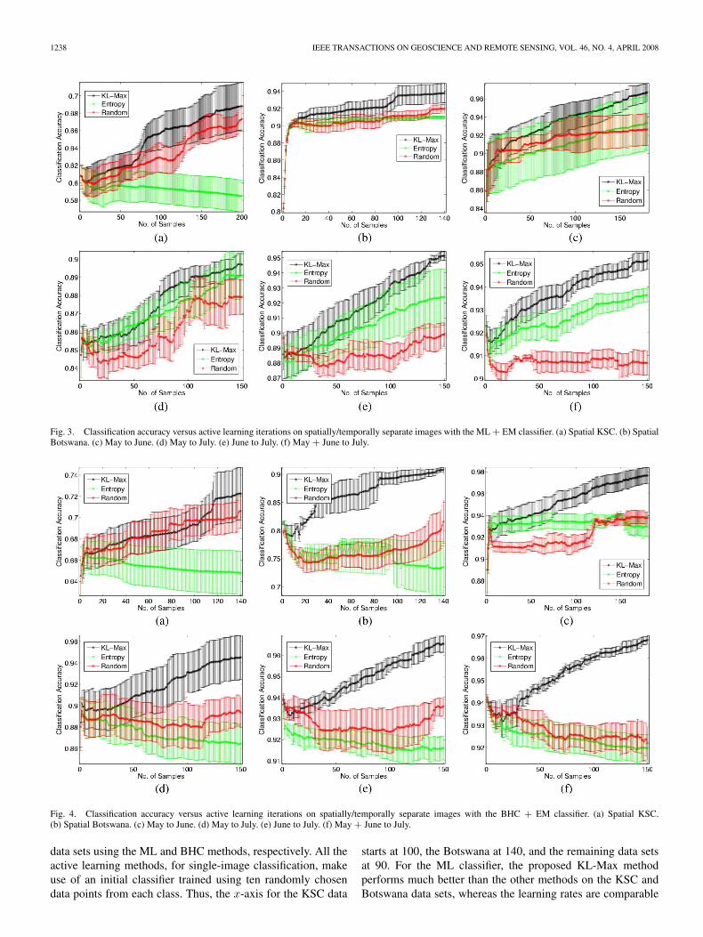
Fig. 3. Classification accuracy versus active learning iterations on spatially/temporally separate images with the ML + EM classifier. (a) Spatial KSC. (b) SpatialBotswana. (c) May to June. (d) May to July. (e) June to July. (f) May + June to July.

Fig. 4. Classification accuracy versus active learning iterations on spatially/temporally separate images with the BHC + EM classifier. (a) Spatial KSC.(b) Spatial Botswana. (c) May to June. (d) May to July. (e) June to July. (f) May + June to July.

data sets using the ML and BHC methods, respectively. All theactive learning methods, for single-image classification, makeuse of an initial classifier trained using ten randomly chosendata points from each class. Thus, the x-axis for the KSC data

starts at 100, the Botswana at 140, and the remaining data setsat 90. For the ML classifier, the proposed KL-Max methodperforms much better than the other methods on the KSC andBotswana data sets, whereas the learning rates are comparable


Fig. 5. Likelihood of classes being chosen by the active learning methods for the May-to-June knowledge transfer problem. (a) Per-class confusion.(b) ML entropy. (c) BHC entropy. (d) ML KL-Max. (e) BHC KL-Max.

to those of the entropy-based approach on the May, June, andJuly data sets. On data sets with a larger number of classes,the entropy-based method performs worse than even randomselection. The poor performance of the entropy-based methodcould be attributed to the fact that focusing on data points thatincrease the future expected entropy results in skewed estimatesof the class distributions.

Similar trends can be observed for the BHC method. Whenthe proposed active learning approach was applied, both BHCand ML classifiers exhibited comparable learning behavior.However, the entropy-based method performed even worse withthe BHC technique for these data sets. A possible reason forthis behavior is the greater dependence of the BHC on theadequacy of the estimated class distributions. Each node in theBHC hierarchy makes use of class distribution estimates for

determining the corresponding Fisher-m extractor and learningdecision boundaries. Hence, skewed class distribution estimateswould have an increasingly adverse effect on classificationaccuracies while traversing down the tree, which results in pooroverall classification accuracies.

B. Knowledge Transfer

The proposed approach seems to be particularly well suitedto the problem of knowledge transfer. Fig. 3 shows the learn-ing rates for the spatially/temporally separated data sets overthe active learning iterations. Note that unlike the single-imagecase, the x-axis for all the data sets in this case starts atzero. The KL-Max method yields higher overall classifica-tion accuracies than the other approaches. The results for the


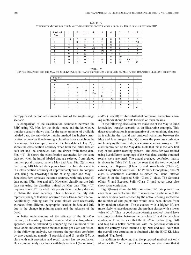
TABLE IVCONFUSION MATRIX FOR THE MAY-TO-JUNE KNOWLEDGE TRANSFER PROBLEM USING SEMISUPERVISED BHC

TABLE VCONFUSION MATRIX FOR THE MAY-TO-JUNE KNOWLEDGE TRANSFER PROBLEM USING BHC KL-MAX AFTER 180 ACTIVE LEARNING ITERATIONS

entropy-based method are similar to those of the single-imagescenario.

A comparison of the classification accuracies between theBHC using KL-Max for the single image and the knowledgetransfer scenario shows that for the same amounts of availablelabeled data, the knowledge transfer method has higher classi-fication accuracies than learning a classifier from scratch on thenew image. For example, consider the July data set. Fig. 2(e)shows the classification accuracy when both the initial labeleddata set and the unlabeled data are drawn from these data.Fig. 4(d)–(f) shows the classification accuracies for the samedata set when the initial labeled data are selected from relatedmultitemporal images, namely May and June. Fig. 2(e) showsthat using 140 labeled data points from the July data resultsin a classification accuracy of approximately 94%. In compar-ison, using the knowledge in the existing June and May +June classifiers achieves the same accuracy with only about 50data points [Fig. 4(e) and (f)]. However, classifying the Julydata set using the classifier trained on May data [Fig. 4(d)]requires about 120 labeled data points from the July data setto obtain the same accuracy. This is because the July datarepresent changes that have occurred over a two-month interval.Additionally, training data for some classes were necessarilyextracted from different geographic locations in June and Julydue to the change in pointing angle and the advance of theflood.

A better understanding of the efficacy of the KL-Maxmethod, for knowledge transfer, compared to the entropy-basedapproach, can be obtained by comparing the likelihood of theclass labels chosen by these methods to the per-class confusion.In the following analysis, we measure the per-class confusionby two quantities, namely (1-precision) and (1-recall) [37]. Aclass with unit precision and recall values has no confusion.Hence, in our analysis, classes with high values of (1-precision)

and/or (1-recall) exhibit substantial confusion, and active learn-ing methods should be able to focus on such classes.

In the following discussion, we make use of the May-to-Juneknowledge transfer scenario as an illustrative example. Thisdata set combination is representative of the remaining data setsas it exhibits the spatial and temporal variations between theMay and June images. Fig. 5(a) shows the per-class confusionin classifying the June data, via semisupervision, using a BHCclassifier trained on the May data. Note that this is the very firststep of the active learning process. The classifier was trainedusing five different samplings of the May data, and the obtainedresults were averaged. The actual averaged confusion matrixis shown in Table IV. It can be seen that the two woodlandclasses, i.e., Riparian (Class 3) and Woodlands (Class 6),exhibit significant confusion. The Primary Floodplain (Class 2)class is sometimes classified as either the Island Interior(Class 5) or the Exposed Soils (Class 9) class. The Savanna(Class 7) and Exposed Soils (Class 9) land cover types alsoshow some confusion.

Fig. 5(b)–(e) shows the lift in selecting 180 data points fromeach class. For each class, the lift is measured as the ratio of thenumber of data points chosen by the active learning method tothe number of data points that would have been chosen fromit by random selection. Those classes with a higher lift aremore likely to have data points chosen than classes with a lowervalue of lift. Thus, a good active learning method should havea strong correlation between the per-class lift and the per-classconfusion. It can be seen that the KL-Max method [Fig. 5(d)and (e)] has a better correlation with the per-class confusionthan the entropy-based method [Fig. 5(b) and (c)]. Note thatthe overall best correlation is obtained with the BHC KL-Maxmethod [Fig. 5(e)].

In addition to showing that the proposed method not onlyidentifies the “correct” problem classes, we also show that it


Fig. 6. Number of data points chosen from each class at different activelearning iterations for the May-to-June knowledge transfer problem.

selects the most informative data points from these classes.Table V shows the averaged confusion matrix obtained by theBHC KL-Max method after 180 active learning iterations. TheKL-Max method eliminates the confusion among all classes ex-cept that of Riparian (Class 3) and Woodlands (Class 6), whichare both tree classes. Fig. 5(e) shows that while the KL-Maxmethod is more likely to select data points from classes 3 and6, the two classes continue to exhibit some confusion. To un-derstand this behavior, consider Fig. 6 showing the distributionof class labels selected after 33, 66, and 100 iterations of asingle active learning run. Note that for classes 2 and 7, theincrease in the number of additional labeled data points, i.e.,between 33 and 100 iterations, is far less than that of classes 3and 6. Thus, one may conclude that for classes 2 and 7, themost informative data points are chosen early on in the activelearning process, which probably is the case for classes 3 and6 as well. However, as we force active learning to proceed,regardless of whether the estimates of class distributions changeacross subsequent iterations, the algorithm continues to selectdata points from the “more confusing” classes 3 and 6.

VI. CONCLUSION

We have proposed a new active learning approach for ef-ficiently updating classifiers built from small quantities oflabeled data. The principle of selecting data points that mostlychange the existing belief in class distributions seems to beparticularly well suited to the scenario in which the distributionsof the classes show spatial (or temporal) variations. The pro-posed method is empirically shown to have better learning ratesthan choosing data points at random and an entropy-based ac-tive learning method regardless of the underlying probabilisticclassifier. This paper can be expanded when more hyperspectraldata are available, especially to determine the effectiveness ofthe active learning-based knowledge transfer framework whenthe spatial/temporal separation of the data sets is systematicallyincreased.

ACKNOWLEDGMENT

The authors would like to thank A. Neunschwander andY. Chen for help in preprocessing the Hyperion data.

REFERENCES

[1] J. S. Pearlman, P. S. Berry, C. C. Segal, J. Shapanski, D. Beiso, andS. L. Carman, “Hyperion: A space-based imaging spectrometer,” IEEETrans. Geosci. Remote Sens., vol. 41, no. 6, pp. 1160–1173, Jun. 2003.

[2] S. Rajan, J. Ghosh, and M. M. Crawford, “An active learning approachto knowledge transfer for hyperspectral data analysis,” in Proc. IGARSS,Denver, CO, 2006, pp. 541–544.

[3] A. P. Dempster, N. M. Laird, and D. B. Rubin, “Maximum likelihoodfrom incomplete data via the EM algorithm,” J. R. Stat. Soc. Ser. B, Stat.Methodol., vol. 39, no. 1, pp. 1–38, 1977.

[4] T. Joachims, “Transductive inference for text classification using supportvector machines,” in Proc. 16th ICML, 1999, pp. 200–209.

[5] M. Seeger, “Learning with labeled and unlabeled data,” Inst. forAdaptive Neural Comput., Univ. Edinburgh, Edinburgh, U.K., Feb. 2001.Tech. Rep.

[6] D. MacKay, “Information-based objective functions for active data selec-tion,” Neural Comput., vol. 4, no. 4, pp. 590–604, Jul. 1992.

[7] B. M. Shahshahani and D. A. Landgrebe, “The effect of unlabeled samplesin reducing the small sample size problem and mitigating the Hughes phe-nomenon,” IEEE Trans. Geosci. Remote Sens., vol. 32, no. 5, pp. 1087–1095, Sep. 1994.

[8] J. T. Morgan, A. Henneguelle, M. M. Crawford, J. Ghosh, andA. Neuenschwander, “Adaptive feature spaces for land cover classifi-cation with limited ground truth,” in Multiple Classifier Systems,Lecture Notes in Computer Science, vol. 2364, F. Roli and J. Kittler, Eds.New York: Springer-Verlag, 2002, pp. 189–200.

[9] J. A. Richards, M. M. Crawford, J. P. Kerkes, S. B. Serpico, andJ. C. Tilton, “Foreword to the special issue on advances in techniquesfor analysis of remotely sensed data,” IEEE Trans. Geosci. Remote Sens.,vol. 43, no. 3, pp. 411–413, Mar. 2005.

[10] Q. Jackson and D. A. Landgrebe, “An adaptive classifier design for high-dimensional data analysis with a limited training data set,” IEEE Trans.Geosci. Remote Sens., vol. 39, no. 12, pp. 2264–2279, Dec. 2001.

[11] M. Dundar and D. A. Landgrebe, “A cost-effective semi-supervised clas-sifier approach with kernels,” IEEE Trans. Geosci. Remote Sens., vol. 42,no. 1, pp. 264–270, Jan. 2004.

[12] B. Jeon and D. A. Landgrebe, “Partially supervised classification usingweighted unsupervised clustering,” IEEE Trans. Geosci. Remote Sens.,vol. 37, no. 2, pp. 1073–1079, Mar. 1999.

[13] P. Mantero, G. Moser, and S. B. Serpico, “Partially supervised classifi-cation of remote sensing images through SVM-based probability densityestimation,” IEEE Trans. Geosci. Remote Sens., vol. 43, no. 3, pp. 559–570, Mar. 2005.

[14] P. H. Swain, “Bayesian classification in a time-varying environment,”IEEE Trans. Syst., Man, Cybern., vol. SMC-8, no. 12, pp. 879–883,Dec. 1978.

[15] Y. Bazi, L. Bruzzone, and F. Melgani, “An approach to unsupervisedchange detection in multi-temporal SAR images based on the general-ized Gaussian distribution,” in Proc. IGARSS, Anchorage, AK, 2004,pp. 1402–1405.

[16] S. B. Serpico, L. Bruzzone, F. Roli, and M. A. Gomarasca, “An automaticapproach for detecting land-cover transitions,” in Proc. IGARSS, Lincoln,NE, 1996, pp. 1382–1384.

[17] B. Jeon and D. A. Landgrebe, “Decision fusion approach for multitem-poral classification,” IEEE Trans. Geosci. Remote Sens., vol. 37, no. 3,pp. 1227–1233, 1999.

[18] B. Jeon and D. A. Landgrebe, “Spatio temporal contextual classificationof remotely sensed multispectral data,” in Proc. IEEE Int. Conf. Syst, Man,Cybern., Los Angeles, CA, 1990, pp. 342–344.

[19] N. Khazenie and M. M. Crawford, “Spatial–temporal autocorrelatedmodel for contextual classification,” IEEE Trans. Geosci. Remote Sens.,vol. 28, no. 4, pp. 529–539, Jul. 1990.

[20] L. Bruzzone and D. F. Prieto, “Unsupervised retraining of a maximumlikelihood classifier for the analysis of multitemporal remote sensingimages,” IEEE Trans. Geosci. Remote Sens., vol. 39, no. 2, pp. 456–460,Feb. 2001.

[21] S. Kumar, J. Ghosh, and M. M. Crawford, “Hierarchical fusion of multipleclassifiers for hyperspectral data analysis,” Pattern Anal. Appl., vol. 5,no. 2, pp. 210–220, 2002.

[22] T. G. Dietterich and G. Bakiri, “Solving multi-class learning problems viaerror-correcting output codes,” J. Artif. Intell. Res., vol. 2, pp. 263–286,1995.

[23] P. Mitra, B. U. Shankar, and S. K. Pal, “Segmentation of multispectralremote sensing images using active support vector machines,” PatternRecognit. Lett., vol. 25, no. 9, pp. 1067–1074, Jul. 2004.


[24] D. Cohn, Z. Gharamani, and M. Jordan, “Active learning with statisticalmodels,” Artif. Intell. Res., vol. 4, pp. 129–145, 1996.

[25] T. M. Cover and J. A. Thomas, Elements of Information Theory.Hoboken, NJ: Wiley, 1991.

[26] N. Roy and A. K. McCallum, “Toward optimal active learning throughsampling estimation of error reduction,” in Proc. 18th ICML, 2001,pp. 441–448.

[27] D. Lewis and W. A. Gale, “A sequential algorithm for training text clas-sifiers,” in Proc. 17th Int. ACM SIGIR Conf. Res. Develop. Inf. Retrieval,1994, pp. 3–12.

[28] H. S. Seung, M. Opper, and H. Smopolinsky, “Query by committee,” inProc. 5th Annu. ACM Workshop Comput. Learning Theory, Pittsburgh,PA, 1992, pp. 287–294.

[29] N. Abe and H. Mamitsuka, “Query learning strategies using boosting andbagging,” in Proc. 15th ICML, 1998, pp. 1–9.

[30] V. S. Iyengar, C. Apte, and T. Zhang, “Active learning using adaptiveresampling,” in Proc. 6th ACM SIGKDD Int. Conf. Knowl. Discovery andData Mining, 2000, pp. 92–98.

[31] M. Saar-Tsechansky and F. J. Provost, “Active learning for class proba-bility estimation and ranking,” in Proc. 17th Int. Joint Conf. Artif. Intell.,2001, pp. 911–920.

[32] P. Melville, S. M. Yang, M. Saar-Tsechansky, and R. J. Mooney, “Activelearning for probability estimation using Jensen–Shannon divergence,” inProc. 16th ECML, 2005, pp. 268–279.

[33] A. K. McCallum and K. Nigam, “Employing EM in pool-based activelearning for text classification,” in Proc. 15th ICML, 1998, pp. 350–358.

[34] I. Muslea, S. Minton, and C. Knoblock, “Active + semi-supervised learn-ing = robust muti-view learning,” in Proc. 19th ICML, Sydney, Australia,2002, pp. 435–442.

[35] Y. D. Rubinstein and T. Hastie, “Discriminative vs informative learning,”in Proc. Knowledge Discovery and Data Mining, 1997, pp. 49–53.

[36] S. Kumar, J. Ghosh, and M. M. Crawford, “Best-bases feature extractionalgorithms for classification of hyperspectral data,” IEEE Trans. Geosci.Remote Sens., vol. 39, no. 7, pp. 1368–1379, Jul. 2001.

[37] C. M. Bishop, Neural Networks for Pattern Recognition. New York:Oxford Univ. Press, 1995.

[38] J. T. Morgan, “Adaptive hierarchical classifier with limited training data,”Ph.D. dissertation, Dept. Mech. Eng., Univ. Texas, Austin, TX, 2002.

[39] J. Ham, Y. Chen, M. M. Crawford, and J. Ghosh, “Investigation of therandom forest framework for classification of hyperspectral data,” IEEETrans. Geosci. Remote Sens., vol. 43, no. 3, pp. 492–501, Mar. 2005.

[40] [Online]. Available: www.lans.ece.utexas.edu/˜rsuju/hyper.pdf

Suju Rajan received the B.E. degree in electronicsand communications engineering from the Univer-sity of Madras, Chennai, India, in 1997, and theM.S. and Ph.D. degrees from the University of Texas,Austin, in 2004 and 2006, respectively.

She is currently with the Department of Electricaland Computer Engineering, The University of Texas.Her research interests primarily lie in machine learn-ing, information retrieval, and data mining.

Joydeep Ghosh (S’87–M’88–SM’02–F’06) re-ceived the B.Tech. degree from the Indian Insti-tute of Technology, Kanpur, in 1983 and the Ph.D.degree from the University of Southern California,Los Angeles, in 1988.

Since 1988, he has been with the Universityof Texas (UT), Austin, where he is currently aSchlumberger Centennial Chair Professor of Elec-trical and Computer Engineering. He is the Founder–Director of the Intelligent Data Exploration andAnalysis Lab (IDEAL). He has published more than

200 refereed papers and 30 book chapters, and co-edited 18 books. His researchinterests primarily lie in intelligent data analysis, data mining and web mining,adaptive multilearner systems, and their applications to a wide variety ofcomplex engineering and AI problems.

Dr. Ghosh is the founding chair of the Data Mining Tech. Committee of theIEEE CI Society. He was the Conference Co-Chair from 1993 to 1996 andfrom 1999 to 2003 for the Artificial Neural Networks in Engineering (ANNIE),the Program Co-Chair for The 2006 SIAM International Conference on DataMining, and the Conference Co-Chair of the 2007 Computational Intelligenceand Data Mining. He was voted the Best Professor by the Software EngineeringExecutive Education Class of 2004 and has given keynote talks at severalinternational forums. He has received 12 best paper awards, including the 2005Best Research Paper from UT from the Co-op Society and the 1992 DarlingtonAward given for the best paper across all publications of the IEEE Circuits andSystems Society.

Melba M. Crawford (M’89–SM’05–F’07) receivedthe B.S. and M.S. degrees in civil engineering fromthe University of Illinois, Urbana, in 1970 and 1973,respectively, and the Ph.D. degree in systems engi-neering from The Ohio State University, Columbus,in 1981.

From 1990 to 2005, she was a faculty memberwith the University of Texas, Austin. She is currentlywith Purdue University, West Lafayette, IN, whereshe is the Director of the Laboratory for Applicationsof Remote Sensing and the Assistant Dean for Inter-

disciplinary Research in the Colleges of Agriculture and Engineering. Sheis the holder of the Purdue Chair of Excellence in Earth Observation. Shehas more than 100 publications in scientific journals, conference proceedings,and technical reports, and is internationally recognized as an expert in thedevelopment of statistical methods for the analysis of hyperspectral and LIDARremote sensing data.

Dr. Crawford was a Jefferson Senior Science Fellow at the U.S. Departmentof State from 2004 to 2005. She is a member of the IEEE Geoscience andRemote Sensing Society, where she is currently the Vice President for Meetingsand Symposia, and an Associate Editor of the IEEE TRANSACTIONS ON

GEOSCIENCE AND REMOTE SENSING. She has also served as a memberof the NASA Earth System Science and Applications Advisory Committee(ESSAAC) and was a member of the NASA EO-1 Science Validation team forthe Advanced Land Imager and Hyperion, which received a NASA OutstandingService Award. She is currently a member of the advisory committee to theNASA Socioeconomic Applications and Data Center at Columbia University,New York, NY.

An Active Learning Approach to Hyperspectral Data Classification

Documents

Transcript of An Active Learning Approach to Hyperspectral Data Classification