An Accelerated First-Order Method for Solving Unconstrained

Polynomial Optimization Problems

Dimitris Bertsimas∗ Robert M. Freund† Xu Andy Sun‡

March 2011

Abstract

Our interest lies in solving large-scale unconstrained polynomial optimization problems. Because

interior-point methods for solving these problems are severely limited by the large-scale, we are

motivated to explore efficient implementations of an accelerated first-order method to solve this class

of problems. By exploiting special structural properties of this problem class, we greatly reduce the

computational cost of the first-order method at each iteration. We report promising computational

results as well as a curious observation about the behavior of the first-order method for unconstrained

polynomial optimization.

1 Introduction

We are interested in solving the unconstrained polynomial optimization problem:

(P ) γ∗ = minx∈Rn

p(x),

where p(x) : Rn → R is a real-valued polynomial in n variables and of even degree d = 2m, where

m is an integer. Polynomial optimization has connections to many fields such as algebraic geometry

[14], the problem of moments [5, 11], and semidefinite programming (SDP) [17]. It has also been a

useful tool in control theory [21], optimized moment inequalities in probability theory [4], combinatorial

optimization [19], and stochastic modeling [7]. However, despite interesting theoretical properties and

rich modeling capabilities, polynomial optimization techniques have not been extensively used in real

∗Sloan School of Management, Massachusetts Institute of Technology, Cambridge, MA 02139, dbertsim@mit.edu.†Sloan School of Management, Massachusetts Institute of Technology, Cambridge, MA 02139, rfreund@mit.edu.‡Operations Research Center, Massachusetts Institute of Technology, Cambridge, MA 02139, sunx@mit.edu.

1

applications. One reason for this is the limitation of current computational schemes for solving large

instances of polynomial optimization problems. Using the most successful solution methodology — the

hierarchy of semidefinite programming ( SDP) relaxations [13][22], the resulting SDP problem involves

a (primal) matrix variable of order(

n+mn

)

×(

n+mn

)

= O(nm × nm) and a (dual) vector variable of

dimension(

n+2mn

)

= O(n2m), which grows exponentially in the degree of the polynomial. Currently,

the most widely used software (such as Gloptipoly [8] and SOSTOOLS [23]) solve the SDP relaxation

by interior-point methods, where the exponential growth in the SDP dimension severely limits the size

of solvable instances.

In this paper, we explore the possibility of improving the practical solvability of polynomial opti-

mization problems. Instead of using powerful but expensive interior-point methods (IPMs), we take

advantage of the recent progress on solving conic optimization problems with first-order algorithms. In

particular, we apply a variant of Nesterov’s accelerated first-order method [26, 1] to the SDP relaxation

of an unconstrained polynomial optimization problem, using a reformulation proposed in Lu [15]. The

key to the success of such an approach depends on the ability to exploit the special structure of the

reformulation in the context of the projection operators that are used in the accelerated first-order

method. To accomplish this, we identify a special property of the SDP reformulation, and we show that

this property enables very fast computation of projections onto a certain affine manifold that arises

in accelerated first-order method. The reduced computational cost of the first-order algorithm is then

demonstrated via numerical experiments, which show that the accelerated first-order method can solve

larger instances than the existing interior-point-method based software. For both 4-degree and 6-degree

polynomials, the first-order method solves instances of dimensions roughly twice as large (in terms of

the number of polynomial variables n) as existing IPM software (namely, the SOS package in SeDuMi)

can handle. The first-order method is also faster than the existing software for medium size problems

when solved to comparable accuracy.

Over the past several years, research on accelerated first-order methods has grown substantially,

especially on the computational frontier of applying such methods to solving large-scale problems (see,

e.g., compressed sensing [15, 3], covariance selection [6, 16], and image processing [2]). However, to

the best of our knowledge, such methods have not been applied to general unconstrained polynomial

optimization. Herein we study the behavior of accelerated first-order methods on solving this important

class of problems. We also discuss a curious observation on the convergence behavior of this method

that is not derivative of the usual convergence analysis.

The paper is organized as follows: In Section 2, we first briefly review the method of SDP relaxation

2

of unconstrained polynomial optimization problems and reformulations that are suitable for applying the

intended accelerated first-order method. We then demonstrate the special structure of the reformulation

that allows for fast computation of the affine manifold projection problem at each iteration. In Section

3 we report computational results and provide a comparison with existing interior-point based methods.

We also provide some interesting observations on the convergence behavior of the accelerated first-order

method.

1.1 Notation and Definitions

Let Sn denote the space of n × n real symmetric matrices, and S

n+ denote the cone of n × n positive

semidefinite matrices. Let � denote the standard ordering on Sn induced by the cone Sn+. For X,Y ∈ S

n,

let X • Y denote the Frobenius inner product, and ‖X‖F denote the induced matrix norm, namely

‖X‖F =√X •X =

√

∑ni=1

∑nj=1

X2ij . For x, y ∈ R

n, let xT y denote the standard Euclidean inner

product, and ‖x‖2 denote the Euclidean norm. More generally, for a finite dimensional inner product

space U, let ‖ · ‖ denote the induced norm. For a compact convex set C ∈ U, define a distance function

dC(u) := min{‖u − v‖| v ∈ C} for all u ∈ U. Define ΠC(u) := argmin{‖u − v‖| v ∈ C}. The “prox”

or squared distance function d2C(u) is a Lipschitz differentiable convex function with Lipschitz constant

L = 2, whose gradient operator is given by ∇ud2C(u) = 2(u−ΠC(u)), see [10].

Let N denote the set of nonnegative integers, and Nnd := {α ∈ N

n| |α| :=∑ni=1

αi ≤ d} for n, d ∈ N

and n > 0. For α = (α1, . . . , αn) ∈ Nn, and x = (x1, . . . , xn) ∈ R

n, let xα denote the monomial

xα11xα22· · · xαn

n of degree |α|. For d = 2m, let

v2m(x) := {1, x1, x2, . . . , xn, x21, x1x2, . . . , x1xn, x22, x2x3, . . . , x2mn } (1.1)

be a basis for the n-variable and degree d = 2m real-valued polynomial, so that we can write

p(x) =∑

α∈Nn

2m

pαxα = pTv2m(x) . (1.2)

Let M denote the number of components of v2m(x), namely M =(

n+2mn

)

. Let N :=(

n+mn

)

. For each

α ∈ Nn2m, let Aα ∈ S

N denote the matrix corresponding the following operator:

Aα(X) := Aα •X =∑

δ

∑

ν=α−δ

Xδν , for all X ∈ SN , (1.3)

where X is indexed by δ, ν ∈ Nnm. The matrices Aα are called the basic moment matrices, which

are used to define the moment matrix M2m(y) of the finite moment sequence y ∈ RM as M2m(y) :=

∑

α∈Nn

2myαAα.

3

A polynomial p(x) is called a sum of squares (SOS) polynomial if p(x) can be written as p(x) =∑s

i=1q2i (x) for some polynomials q1(x), . . . , qs(x).

2 SOS Formulation, Reformulation, and Accelerated First-Order Method

2.1 SOS relaxation

For a given n-variable d = 2m-degree polynomial p(x), we consider the unconstrained polynomial

optimization problem:

(P ) γ∗ = minx∈Rn

p(x),

and there is no loss of generality in assuming that p(x) has zero constant term. Problem (P ) admits

the following SOS relaxation:

γ∗sos = maxγ∈R

γ

s.t. p(x)− γ is SOS. (2.1)

In general, we have γ∗sos ≤ γ∗. When p(x)− γ∗ is an SOS polynomial, then γ∗sos = γ∗ [13, Theorem 3.2].

The SOS constraint can be written as:

p(x)− γ =

s∑

i=1

q2i (x) =

s∑

i=1

vm(x)T qiqTi vm(x) = vm(x)T

(

s∑

i=1

qiqTi

)

vm(x) = vm(x)TXvm(x),

for some polynomials qi(x) of degree at most m, and X ∈ SN+ . Matching monomial coefficients on both

sides above, it follows that X must satisfy:

X00 = −γ,∑

δ

∑

ν=α−δ Xδν = pα for α ∈ Nn2m, |α| > 0,

(2.2)

which yields the following SDP formulation of (2.1):

γ∗p = minX∈SN

A0 •X

s.t. Aα •X = pα for α ∈ Nn2m, |α| > 0, (2.3)

X � 0.

4

The dual of (2.3) is:

γ∗d = maxy∈RM−1,S∈SN

∑

α∈Nn

2m,|α|>0

pαyα,

s.t.∑

α∈Nn

2m,|α|>0

yαAα + S = A0, (2.4)

S � 0.

We have γ∗p = −γ∗sos. If (2.3) has a feasible solution, then there is no duality gap between (2.3) and

(2.4), i.e., γ∗p = γ∗d , see [13, Proposition 3.1].

2.2 Reformulations of the SDP problem

In order to apply an accelerated first-order method to solve (2.3) and (2.4), one needs to reformulate these

problems so that the resulting reformulated feasible region is a simple convex set for which computation

of projections can be done very efficiently. Several such reformulations have been proposed in the

recent literature, see for example [12, 9, 15]. In particular, Lu [15] has derived a detailed worst-case

complexity analysis and comparison of the cited proposals, and successfully applied one recommended

scheme to solve a class of linear programs, MaxCut SDP relaxation, and the Lovasz capacity problem.

For completeness, we present these reformulations and choose a scheme (different from that in [15]) here

that is most suited for computing solutions of (2.3)-(2.4).

Herein we are concerned with those instances of (P ) for which p(x)− γ∗ is SOS. Hence we presume

that (2.3) is feasible, in which case strong duality holds in (2.3) and (2.4). We then write the optimality

conditions for the primal-dual pair as follows:

Aα •X = pα, for all α ∈ Nn2m, |α| > 0, (2.5)

∑

α∈Nn

2m,|α|>0

yαAα + S = A0, (2.6)

A0 •X = pT y, (2.7)

X,S ∈ SN+ , y ∈ R

M−1. (2.8)

Note that any solution of (2.5)-(2.8) is an optimal primal-dual solution of (2.3) and (2.4), and vice versa.

Define the finite dimensional space U := SN × S

N × RM−1. For u = (X,S, y), u = (X, S, y) ∈ U, define

the inner product u • u := X • X + S • S + yT y. The solution set of equations (2.5)-(2.7) define an

affine subspace L ⊂ U, and the inclusion (2.8) defines a convex cone K := SN+ × S

N+ × R

M−1 ⊂ U. We

5

represent L in a more compact form by introducing a linear operator A : SN → RM−1 and its adjoint

A∗ : RM−1 → SN defined as follows:

z = A(X) where zα := Aα •X, for all α ∈ Nn2m, |α| > 0, (2.9)

v = A∗(y) where v :=∑

α∈Nn

2m,|α|>0

yαAα . (2.10)

Here the matrices Aα are the basic moment matrices defined in Section 1.1. Similarly, consider another

linear operator A0 : SN → R defined as A0(X) := A0 •X for all X ∈ S

N . We also denote I1 : SN → SN

as the identity operator. Using all of this notation, the subspace L defined above as the solution of the

equations (2.5)-(2.7) can be conveniently represented as L := {u ∈ U : Eu = q} where

E =

A 0 0

0 I1 A∗

A0 0 −pT

, u =

X

S

y

, q =

p

A0

0

. (2.11)

Note of course that solving (2.5)-(2.8) (and hence solving (2.3) and (2.4)) is equivalent to finding a

point u ∈ L ∩K, for which any of the following reformulations are possible candidates for computing a

solution via an accelerated first-order method:

min{f1(u) := ‖Eu− q‖22 : u ∈ K}, (2.12)

min{f2(u) := d2L(u) + d2K(u) : u ∈ U}, (2.13)

min{f3(u) := d2L(u) : u ∈ K}, and/or (2.14)

min{f4(u) := d2K(u) : u ∈ L}. (2.15)

Here dL and dK are the distance functions defined in Section 1.1. Formulation (2.12) was first proposed

in [9], (2.13) was studied in [12], and (2.14) and (2.15) were proposed in [15]. Scheme (2.15) is the most

efficient from the vantage point of worst-case complexity analysis, especially when ‖E‖ is large, see [15].However, when applied to the class of polynomial optimization problems under consideration herein,

we have observed that (2.14) converges faster than (2.15), as we look at a converging sequence different

from the one in the theoretical analysis (see Section 3.3 for more discussion). We therefore have chosen

scheme (2.14) for implementation and extensive computational experiments, which we report in Section

3 with further discussion.

6

2.3 An Accelerated First-Order Method

We wish to solve problem (2.14), namely:

min f(u) := d2L(u)

s.t. u ∈ K ,(2.16)

which, under the presumption that p(x) − γ∗ is SOS, is an equivalent reformulation of (2.5)-(2.8) and

hence of (2.3)-(2.4). Here the objective function is the squared distance function of a point to the affine

subspace L. As introduced in Section 1.1, d2L(u) has Lipschitz continuous derivative with Lipschitz

constant L = 2. We use the following accelerated first-order method (AFOM), which was first presented

and analyzed in [1] in a more general setting, but is stated here as presented for the specific setting of

solving (2.16) treated in [15]:

Accelerated First-Order Method (AFOM):

(0) Choose u0 = u0 ∈ K, k ← 0.

(1) Compute uk := 2

k+2uk +

kk+2

uk.

(2) Compute (uk+1, uk+1) ∈ K ×K as follows:

uk+1 := ΠK(uk − k+2

2(uk −ΠL(uk))),

uk+1 :=2

k+2uk+1 +

kk+2

uk.

(3) k ← k + 1, and go to (1).

Note that each iteration of AFOM requires the computation of two projections: ΠL(u) which projects u

onto the affine subspace L, and ΠK(u) which projects u = (X,S, u) onto the cone K := SN+×SN+×RM−1.

Computing ΠK(u) requires computing an eigenvalue decomposition of the two symmetric matrices X

and S; fortunately existing numerical packages are quite efficient for this task, see for example the

eig function in Matlab, which works very effectively for matrices with several thousand rows/columns.

Computing the projection ΠL(u) is typically quite costly, but as we show herein in Section 2.4, the special

structure of the unconstrained polynomial optimization problem can be exploited to substantially speed

up the computation of this projection.

Algorithm AFOM has the following convergence guarantee, originally proved in [1] but stated below

from [15] in the context of problem (2.16):

Theorem 1. [1], [15]. Let {uk} be the sequence generated by algorithm AFOM applied to (2.16) and

let u∗ be any optimal solution of (2.16). For any given ε > 0, dL(uk) ≤ ε can be obtained in at most⌈

2‖u∗ − u0‖ε

⌉

iterations.

7

2.4 Special Structure of (P ) and Improved Efficiency of Projection onto L

In this subsection, we identify and then exploit special structure of the SDP formulation of the un-

constrained polynomial optimization problem, namely the orthogonality property of the basic moment

matrices. This special structure enables a significant speed-up of the projection ΠL used in the acceler-

ated first-order method. We demonstrate easily computable formulas for ΠL and we demonstrate that

this computation uses O(N2), which represents a speed-up of O(M2) operations over the traditional

cost (namely O(M2N2)) for computing the projection.

Lemma 1. For all α ∈ Nn2m, the basic moment matrices Aα are orthogonal to one another. The linear

operator D := AA∗ : RM−1 → RM−1 is diagonal, whose α-th diagonal component is Dα = Aα •Aα and

satisfies 1 ≤ Dα ≤ N for all α ∈ Nn2m satisfying |α| > 0. Therefore

1. A(A0) = 0, equivalently AA∗0 = 0,

2. (AA∗)−1 = D−1

3. (I1 +A∗A)−1 = I1 −A∗(I2 +D)−1A,

4. A(I1 +A∗A)−1 = (I2 +D)−1A, and A(I1 +A∗A)−1(A0) = 0,

5. (I1 +A∗A)−1A∗ = A∗(I2 +D)−1,

6. A(I1 +A∗A)−1A∗ = D(I2 +D)−1, and

7. I2 −A(I1 +A∗A)−1A∗ = (I2 +D)−1,

where the identity operators are defined as I1 : SN → SN and I2 : RM−1 → R

M−1.

Proof. Recall the definition of the basic moment matrix Aα: for all δ, ν ∈ Nnm, the (δ, ν)-entry of Aα is

Aα(δ, ν) =

1 if δ + ν = α,

0 otherwise.

(2.17)

Therefore, the basic moment matrices are orthogonal to each other, i.e., for all α, β ∈ Nn2m,

Aα • Aβ =

0 α 6= β,

nα ≥ 1 α = β,

(2.18)

8

where nα is the number of 1’s in the matrix Aα. Let z := AA∗(y), then the α-entry of z is given by:

zα =∑

ν

yνAν • Aα = nαyα. (2.19)

Therefore D := AA∗ is a diagonal operator, in which the α-entry on the diagonal is Dα = nα. Since

nα = Aα •Aα, it follows that nα is equal to the number of different ways that α can be decomposed as

α = δ+ ν for δ, ν ∈ Nnm. Since there are in total N different δ’s in N

nm, it also follows that 1 ≤ nα ≤ N .

Item (1.) follows from the orthogonality of the basic moment matrices, and (2.) follows since Dα =

nα ≥ 1 for all α ∈ Nn2m. Item (3.) follows from the Sherman-Morrison-Woodbury identity:

(I1 +A∗A)−1 = I1 −A∗(I2 +AA∗)−1A (2.20)

and then substituting in (2.). To prove the first part of (4.) we premultiply (3.) by A and derive:

A(I1 +A∗A)−1 = A(I1 −A∗(I2 +D)−1A) = A−D(I2 +D)−1A = (I2 +D)−1A,

and the second part of (4.) follows the first part using AA∗0 = 0 from (1.). Item (5.) is simply the adjoint

of the first identity of (4.). Item (6.) follows from (5.) by premultiplying (5.) by A, and (7.) follows

from (6.) by rearranging and simplifying terms.

Remark 1. The orthogonality of basic moment matrices is implied by an even stronger property of

these matrices involving their support indices. Let Sα denote the support of Aα, namely Sα := {(δ, ν) ∈Nnm × N

nm : Aα(δ, ν) 6= 0}. Then it follows that Sα ∩ Sβ = ∅ for α 6= β, which in turn implies the

orthogonality of basic moment matrices.

Lemma 1 allows improved computation of the projection ΠL, as we now show.

Lemma 2. Let u = (X,S, y) ∈ U be given, and let (X, S, y) := ΠL(u). Then the following is a valid

method for computing (X, S, y). First compute the scalars:

ξ ← 1 + pT (I2 +D)−1p, (2.21)

η ← A0 •X − pT (I2 +D)−1y + pT (I2 +D)−1A(S), (2.22)

r← η/ξ. (2.23)

Then compute ΠL(u) as follows:

X = X −A∗D−1(A(X) − p)− rA0, (2.24)

S = A∗(I2 +D)−1(A(S)− y − rp) +A0, (2.25)

y = (I2 +D)−1(−A(S) + y + rp). (2.26)

9

Proof. Recalling the definition of E in (2.11), we note that u = (X, S, y) along with Lagrange multipliers

λ = (w, V , r) ∈ RM−1 × S

N × R are a solution of the following normal equations:

E(u) = q and u− u = E∗λ. (2.27)

Indeed, it is sufficient to determine λ that solves:

EE∗λ = Eu− q, (2.28)

and then to assign

u = u− E∗λ. (2.29)

Using (2.11) and the results in Lemma 1, we obtain:

EE∗ =

AA∗ 0 AA∗0

0 I1 +A∗A −A∗(p)

A0A∗ −pTA A0A∗0 + pTp

=

AA∗ 0 0

0 I1 +A∗A −A∗(p)

0 −pTA 1 + pT p

, (2.30)

therefore the system (2.28) can be written as:

AA∗ 0 0

0 I1 +A∗A −A∗(p)

0 −pTA 1 + pTp

w

V

r

=

A(X)− p

S +A∗(y)−A0

A0 •X − pT y

. (2.31)

It is straightforward to check that the following computations involving auxiliary scalars ξ and η yield

a solution to (2.31):

w ← (AA∗)−1(A(X)− p) (2.32)

ξ ← 1 + pT p− pTA(I1 +A∗A)−1A∗(p) (2.33)

η ← A0 •X − pT y + pTA(I1 +A∗A)−1(S +A∗(y)−A0) (2.34)

r ← η/ξ (2.35)

V ← (I1 +A∗A)−1(S +A∗y −A0 +A∗(p)r). (2.36)

We then use (2.29) to compute u = (X, S, y) as follows:

X ← X −A∗w − rA0 = X −A∗(AA∗)−1(A(X)− p)− rA0 (2.37)

S ← S − V = S − (I1 +A∗A)−1(S −A0 +A∗(y + rp)) (2.38)

y ← y −AV + rp = y + rp−A(I1 +A∗A)−1(S +A∗(y + rp)−A0) (2.39)

10

Summarizing, we have shown that (2.32)-(2.39) solve the normal equations (2.27) and hence (2.37)-

(2.39) are valid formulas for the projection ΠL(u). We now show that these formulas can alternatively

be computed using (2.21)-(2.26). To derive (2.21), we have from (2.33) and (7.) of Lemma 1:

ξ = 1 + pT [I2 −A(I1 +A∗A)−1A∗]p = 1 + pT (I2 +D)−1p .

To derive (2.22), we have from (2.34) and (7.) and (4.) of Lemma 1:

η = A0•X−pT [I2−A(I1+A∗A)−1A∗]y+pTA(I1+A∗A)−1(S−A0) = A0•X−pT (I2+D)−1y+pT (I2+D)−1A(S).

Equations (2.23) and (2.35) are identical, and to derive (2.24), we have from (2.37) and (2.) of Lemma

1:

X = X −A∗D−1(A(X)− p)− rA0.

To derive (2.25), we have from (2.38) and (5.), (3.), and (1.) of Lemma 1:

S = S − (I1 +A∗A)−1(S −A0 +A∗(y + rp))

= [I1 − (I1 +A∗A)−1](S) − (I1 +A∗A)−1A∗(y + rp) + (I1 +A∗A)−1(A0)

= A∗(I2 +D)−1A(S)−A∗(I2 +D)−1(y + rp) +A0.

To derive (2.26), we have from (2.39) and (7.) and (4.) of Lemma 1:

y = [I2 −A(I1 +A∗A)−1A∗](y + rp)−A(I1 +A∗A)−1(S) +A(I1 +A∗A)−1(A0)

= (I2 +D)−1(y + rp)− (I2 +D)−1A(S).

Remark 2. The above computations are numerically well-behaved. To see this, note that there are

no explicit matrix solves, so the issue of solving simultaneous equations is avoided. Second, note that

divisors involve either ξ or the (diagonal) components Dα of D. From (2.21) we see that ξ is bounded

from above and below as

1 ≤ ξ ≤ 1 +1

2‖p‖2 , (2.40)

whereby division by ξ is well-behaved relative to the data p. It also follows from Lemma 1 that

1 ≤ Dα ≤ N, (2.41)

whereby working with D−1 and/or (I2 + D)−1 are also well-behaved relative to the dimension N of the

SDP.

11

The computational cost of computing ΠL(u) using Lemma 2 is bounded from above using the

following lemma.

Lemma 3. The computation of ΠL(u) requires O(N2) arithmetic operations.

Proof. From Lemma 2, the computation of ΠL(u) involves computations with A(·), A∗(·), D−1(·),(I2 + D)−1(·), matrix additions, and vector inner products. These last two involve O(N2) and O(M)

arithmetic operations, respectively. From Remark 1, we observe that A(X) adds the entries of X and

accesses each entry exactly once, so is O(N2) additions. Similarly, A∗(y) forms an N × N matrix by

assigning the entries of y to specific locations, and involves O(N2) operations. Since D is diagonal and

has M positive diagonal elements, D−1(·) and (I2 + D)−1(·) involve M multiplications. Finally, since

N2 ≥ M (this can be seen from the fact that A∗(y) maps exclusive components of y into entries of an

N ×N matrix), the computation of ΠL(u) requires O(N2) arithmetic operations.

Let us now contrast the above bound with the more general case. Consider a general SDP problem

with primal-and-dual decision variables in SN × S

N ×RM−1. From (2.28), computing ΠL involves (at a

minimum) solving systems of equations with the operator AA∗, which requires O(M2N2) operations to

form and O(M3) operations to solve, so the total computational effort is O(M3 +M2N2) = O(M2N2)

operations. Here we see that by identifying and exploiting the structure of the SDP for unconstrained

polynomial optimization, we reduce the computational cost of computing ΠL(u) by a factor of O(M2).

This saving is substantial especially for high degree polynomials, since M =(

n+dn

)

= O(nd) grows

exponentially in the degree d of the polynomial.

3 Computational Results, and Discussion

In this section, we present computational results for the accelerated first-order method AFOM and

compare these results to those of the SeDuMi sossolve interior-point method (IPM) on unconstrained

polynomial optimization problems of degree d = 4 and d = 6. The AFOM is implemented in Matlab

R2008, and the SeDuMi package is version 1.1. The computational platform is a laptop with an Intel

Core(TM) 2Duo 2.50GHz CPU and 3GB memory.

3.1 Generating instances of polynomials

We generated instances of polynomials p(x) in n variables and of degree d = 2m for m = 2 and

m = 3. Each instance was generated randomly as follows. We first chose a random point x∗ uniformly

12

distributed in [−1, 1]n, and then generated the coefficients of k polynomials qi(x) in n variables and

degree m for i = 1, 2, . . . , k, using a uniform distribution on [0, 3]. We then set γ∗ := −∑ki=1

qi(x∗)2

and p(x) =∑k

i=1(qi(x)− qi(x

∗))2 + γ∗. The resulting polynomial p(x) satisfies γ∗ = minx∈Rn p(x) and

p(x) − γ∗ is an SOS polynomial, and furthermore p(x) has zero constant term since p(0) = 0. We set

k = 4 for all instances. The resulting instances have fully dense coefficient vectors p ∈ RM−1. When

generating the 6-degree polynomials, we wanted the polynomials to have a density of coefficients of

10% on average. This was accomplished by suitably controlling the density of the coefficients of the

polynomials qi(x) for i = 1, 2, . . . , k.

3.2 Algorithm Stopping Rules

Both AFOM and the SeDuMi IPM seek to solve the primal/dual SDP instance pair (2.3)-(2.4). We use

SeDuMi’s stoppping rule, see [25], which we briefly review herein. Using the notation of conic convex

optimization, we re-write the primal and dual (2.3)-(2.4) in the standard linear conic optimization

format:

(P ) minx

cTx s.t. Ax = b, x ∈ C ,

(D) maxy,z

bT y s.t. A∗y + z = c, z ∈ C∗ ,

with correspondence b ≡ p, Ax ≡ A(X), cTx ≡ A0 •X, and C,C∗ ≡ SN+ . SeDuMi solves a homogeneous

self-dual (HSD) embedding model until the primal infeasibility, dual infeasibility, and the duality gap

of the current trial iterate (x, y, z) (which automatically satisfies the cone inclusions x ∈ C, z ∈ C∗) are

small. More specifically, define:

rp := b−Ax (primal infeasibility gap)

rd := AT y + z − c (dual infeasibility gap)

rg := cT x− bT y (duality gap) .

SeDuMi’s stopping criterion is:

2‖rp‖∞

1 + ‖b‖∞+ 2

‖rd‖∞1 + ‖c‖∞

+(rg)

+

max(|cT x|, |bT y|, 0.001τ ) ≤ ε .

Here ε is the specified tolerance. The denominator of the third term above depends on the value τ of a

scaling variable τ in the HSD model, see [25]. Since the AFOM does not have any such scaling variable,

we modify the above stopping rule when applied to AFOM to be:

2‖rp‖∞

1 + ‖b‖∞+ 2

‖rd‖∞1 + ‖c‖∞

+(rg)

+

max(|cT x|, |bT y|) ≤ ε.

13

Note that the stopping criterion for AFOM is (marginally) more conservative than that of IPM due to

the absence of the component involving τ in the denominator of the third term above. The stopping

rule tolerance ε is set to 10−4 for all of our computational experiments. Returning to the notation

of the SDP primal and dual problems (2.3)-(2.4) and letting u = (X,S, y) ∈ K be a current iterate

of either AFOM or IPM, then our output of interest is Objective Gap := |pT y + γ∗|, which measures

the objective function value gap between the current dual (near-feasible) solution, namely (−pT y), andthe true global optimal value of the polynomial γ∗. For AFOM, according to Theorem 1, the iterate

sequence uk satisfies the convergence bound, which suggests we should compute Objective Gap using

|pT yk + γ∗|. However, we have observed that dL(uk) also consistently obeys the theoretical convergence

rate of Theorem 1, and that both dL(uk) and |pT yk+γ∗| converge to zero much faster than does dL(uk)

and |pT yk + γ∗|. For this reason we compute Objective Gap using |pT yk + γ∗| and report our results

using the uk = (Xk, Sk, yk) sequence.

Our computational results for 4-degree and 6-degree polynomials are presented in Tables 1 and

Table 2, respectively. In each of these tables, the left-most column displays the dimension n of the

optimization variable x, followed by the size dimensions N and M for the SDP instances (2.3)-(2.4).

The fourth column shows the number of sample instances that were generated for each value of n,

where of necessity we limited the number of sample instances when the dimension n of the problems

(and hence the dimensions N and M of the SDP problems (2.3)-(2.4)) were larger.

For small size problems, IPM runs faster than AFOM. However, AFOM computation time dominates

IPM computation time for n ≥ 12 and n ≥ 8 for 4-degree polynomials and 6-degree polynomials,

respectively. More importantly, since AFOM has much lower memory requirements, AFOM is able to

solve problems in much larger dimension n than IPM (about twice as large for both 4-degree and 6-

degree polynomials). This extends the practical solvability of the SDP representation of the polynomial

optimization problems. For 4-degree polynomials, IPM produces slightly better Objective Gap values,

but no such difference is discernable for 6-degree polynomials. Figure 1 and Figure 2 illustrate the

computation time results in graphical form for 4-degree and 6-degree polynomials, respectively.

One of the generic advantages of interior-point methods is the very low variability in the number of

iterations, and hence in computational burden. By contrast, AFOM has higher variability in terms of

both computation time and Objective Gap values. Such variability is illustrated in the histogram plots

in Figure 3. The histograms in subfigures (a) and (b) show AFOM computation time and Objective

Gap values for the s = 50 sample instances of 4-degree polynomials in dimension n = 19, respectively.

The histograms in subfigures (c) and (d) show AFOM computation time and Objective Gap values for

14

AFOM Performance IPM Performance

SDP Size Time (seconds) Objective Gap Iterations Time (seconds) Objective Gap Iterations

n N M s Median Average Median Average Median Average Median Average Median Average Median

2 6 15 100 2.96E-1 3.9E-1 1.77E-3 1.62E-3 820.0 1068.2 1.13 1.14 1.83E-4 3.98E-4 7

3 10 35 100 1.04 1.66 2.57E-3 2.17E-3 2113.5 3276.9 1.17 1.18 5.70E-4 7.50E-4 8

4 15 70 100 6.35 7.29 4.93E-3 5.15E-3 8416.0 9599.5 1.22 1.22 8.51E-4 1.35E-3 9

5 21 126 100 52.69 36.92 9.10E-3 1.36E-3 19955.5 13661.5 1.40 1.40 4.20E-4 8.63E-4 10

6 28 210 100 11.09 30.22 1.36E-2 8.10E-3 2432.5 6662.8 1.53 1.52 4.45E-4 9.38E-4 10

7 36 330 100 11.31 28.06 8.12E-3 1.18E-2 1624.0 3974.4 1.83 1.84 4.06E-4 9.35E-4 10

8 45 495 100 12.56 23.42 3.09E-3 8.19E-3 1223.5 2311.9 2.57 2.59 6.46E-4 1.09E-3 11

9 55 715 100 14.56 23.22 1.41E-3 4.13E-3 952.0 1151.3 6.86 6.85 6.06E-4 1.36E-3 11

10 66 1001 100 21.42 27.61 1.42E-3 2.93E-3 970.0 1282.1 13.19 13.10 5.21E-4 1.06E-3 11

11 78 1365 100 33.24 40.55 1.74E-3 3.05E-3 1139.5 1401.5 27.40 27.38 5.12E-4 1.28E-3 11

12 91 1820 100 55.17 60.18 1.76E-3 2.76E-3 1240.0 1389.7 64.07 63.54 7.32E-4 1.25E-3 11

13 105 2380 100 82.70 91.12 1.49E-3 2.37E-3 1398.0 1530.0 139.11 138.90 4.09E-4 1.34E-3 12

14 120 3060 100 128.08 141.19 3.90E-3 2.83E-3 1609.0 1781.5 287.70 294.00 8.06E-4 2.53E-3 12

15 136 3876 50 168.99 184.77 3.66E-3 4.63E-3 1693.5 2225.6 575.60 592.70 5.42E-4 2.63E-3 12

16 153 4845 50 263.76 312.94 3.09E-3 6.09E-3 1963.0 2325.8 \ \ \ \ \

17 171 5985 50 385.48 414.21 3.03E-3 5.70E-3 2170.5 2357.6 \ \ \ \ \

18 190 7315 50 586.72 664.94 4.35E-4 6.48E-3 2521.0 2912.0 \ \ \ \ \

19 210 8855 50 833.10 923.29 5.45E-3 9.45E-3 2741.5 3002.7 \ \ \ \ \

20 231 10626 20 1083.90 1125.41 4.60E-3 9.93E-3 3011.0 3097.5 \ \ \ \ \

25 351 23751 15 4682.34 5271.75 8.32E-3 2.13E-2 4595.0 5116.7 \ \ \ \ \

30 496 46376 15 21323.53 21837.43 3.96E-5 5.28E-5 6466.7 6351.5 \ \ \ \ \

Table 1: Computational results for degree-4 polynomials. n is the dimension of the variable x, and s is

the number of sample instances. The stopping rule tolerance is ε = 10−4 for both AFOM and IPM. For

n > 15, IPM fails due to memory requirements.

AFOM Performance IPM Performance

SDP Size Time (seconds) Objective Gap Iterations Time (seconds) Objective Gap Iterations

n N M s Median Average Median Average Median Average Median Average Median Average Median

2 10 28 100 0.47 2.00 3.94E-5 1.14E-4 753.0 3398.9 1.76 1.76 2.14E-5 6.94E-5 7

3 20 84 100 5.09 8.63 8.50E-5 1.72E-4 2384.5 4053.3 1.75 1.75 1.21E-4 2.40E-4 9

4 35 210 100 29.23 37.74 5.41E-4 6.24E-4 5227.5 6719.8 1.93 1.94 4.23E-4 5.98E-4 10

5 56 462 100 78.15 101.38 1.38E-3 1.35E-3 5924.5 7691.5 3.23 3.79 1.89E-4 3.59E-4 10

6 84 924 100 48.76 79.28 1.45E-3 1.36E-3 1529.0 2420.5 10.19 10.13 1.26E-4 2.47E-4 10

7 120 1716 100 48.23 67.14 1.67E-4 8.96E-4 709.5 995.2 49.94 47.90 2.26E-4 3.62E-4 10

8 165 3003 100 67.01 78.35 9.0E-5 3.81E-4 429.5 506.7 231.50 231.53 2.56E-4 5.42E-4 10

9 220 5005 100 123.34 137.42 1.03E-4 3.13E-4 372.5 427.6 1048.44 1063.78 2.64E-4 6.07E-4 11

10 286 8008 60 229.26 250.46 1.50E-4 3.96E-4 404.6 373.0 \ \ \ \ \

11 364 12376 50 471.12 478.16 1.38E-4 3.73E-4 439.5 448.3 \ \ \ \ \

12 455 18564 50 778.63 835.25 1.83E-4 6.49E-4 478.0 516.0 \ \ \ \ \

13 560 27132 10 1380.52 1404.66 9.83E-5 2.16E-4 521.5 538.7 \ \ \ \ \

14 680 38760 10 2944.96 3002.31 8.31E-4 1.01E-3 707.5 725.5 \ \ \ \ \

15 816 54264 10 5393.01 5754.98 5.64E-4 7.91E-4 799.5 859.2 \ \ \ \ \

16 969 74613 10 10041.98 10703.34 6.91E-4 1.40E-3 962.0 1017.3 \ \ \ \ \

Table 2: Computational results for degree-6 polynomials. n is the dimension of the variable x, and s is

the number of sample instances. The stopping rule tolerance is ε = 10−4 for both AFOM and IPM. For

n > 9, IPM fails due to memory requirements.

15

5 10 15 20 25 30

100

101

102

103

104

105

Dimension n

Run

ning

Tim

e (s

econ

ds)

Median and Average Running Time for Degree−4 Polynomials

AFOM−medianAFOM−averageIPM−medianIPM−average

Figure 1: Graph of the median and average running times (in seconds) of AFOM and IPM for degree-4

polynomials in n variables. The values for IPM end in the middle of the graph where IPM fails due to

excessive memory requirements.

2 4 6 8 10 12 14 16

100

101

102

103

104

105

Dimension n

Run

ning

Tim

e (s

econ

ds)

Median and Average Running Time for Degree−6 Polynomials

AFOM−medianAFOM−averageIPM−medianIPM−average

Figure 2: Graph of the median and average running times (in seconds) of AFOM and IPM for degree-6

polynomials in n variables. The values for IPM end in the middle of the graph where IPM fails due to

excessive memory requirements.

16

the s = 50 sample instances of 6-degree polynomials in dimension n = 12, respectively. Observe that

tails and outliers contribute to the higher variation in the performance AFOM in these two metrics.

600 800 1000 1200 1400 1600 1800 2000 2200 24000

0.05

0.1

0.15

0.2

0.25

0.3

0.35

0.4

0.45

0.5

Running Time (seconds)

Fre

quen

cy

(a) Histogram of AFOM running times for

4-degree polynomials in dimension n = 19.

0 0.01 0.02 0.03 0.04 0.050

0.05

0.1

0.15

0.2

0.25

0.3

0.35

0.4

0.45

Objective Gap

Fre

quen

cy

(b) Histogram of AFOM Objective Gap

values for 4-degree polynomials in dimen-

sion n = 19.

600 800 1000 1200 1400 1600 1800 2000 2200 2400 26000

0.1

0.2

0.3

0.4

0.5

0.6

Running Time (seconds)

Fre

quen

cy

(c) Histogram of AFOM running time for

6-degree polynomials in dimension n = 12.

0 0.002 0.004 0.006 0.008 0.01 0.012 0.014 0.016 0.0180

0.1

0.2

0.3

0.4

0.5

0.6

0.7

0.8

0.9

1

Objective Gap

Fre

quen

cy

(d) Histogram of AFOM Objective Gap

values for 6-degree polynomials in dimen-

sion n = 12.

Figure 3: Histograms illustrating variability in running times (Subfigures (a) and (c)) and Objective

Gap values (Subfigures (b) and (d)) of AFOM for 4-degree polynomials and 6-degree polynomials.

3.3 A curious observation

In its simplest form, a traditional first-order (gradient) algorithm produces one sequence of points, where

the next point is determined from the current point by taking a step in the direction of the negative

of the gradient of the current point, according to some specified step-size rule. A crucial difference

between the modern class of accelerated first-order methods and the traditional algorithm is that the

accelerated first-order methods involve more than one sequence in the gradient descent scheme. In

[27, page 80], Nesterov devised a very simple accelerated first-order method with two sequences. The

17

method used in this paper is a variant of Nesterov’s original algorithm, and constructs three sequences–

namely {uk}, {uk}, and {uk}. The convergence analysis establishes the O(1/ε) convergence rate of the

objective function in terms of the sequence values of {uk}. From our computational experiments, we

observe that both dL(uk) and dL(uk) closely follow the theoretical rate O(1/ε).

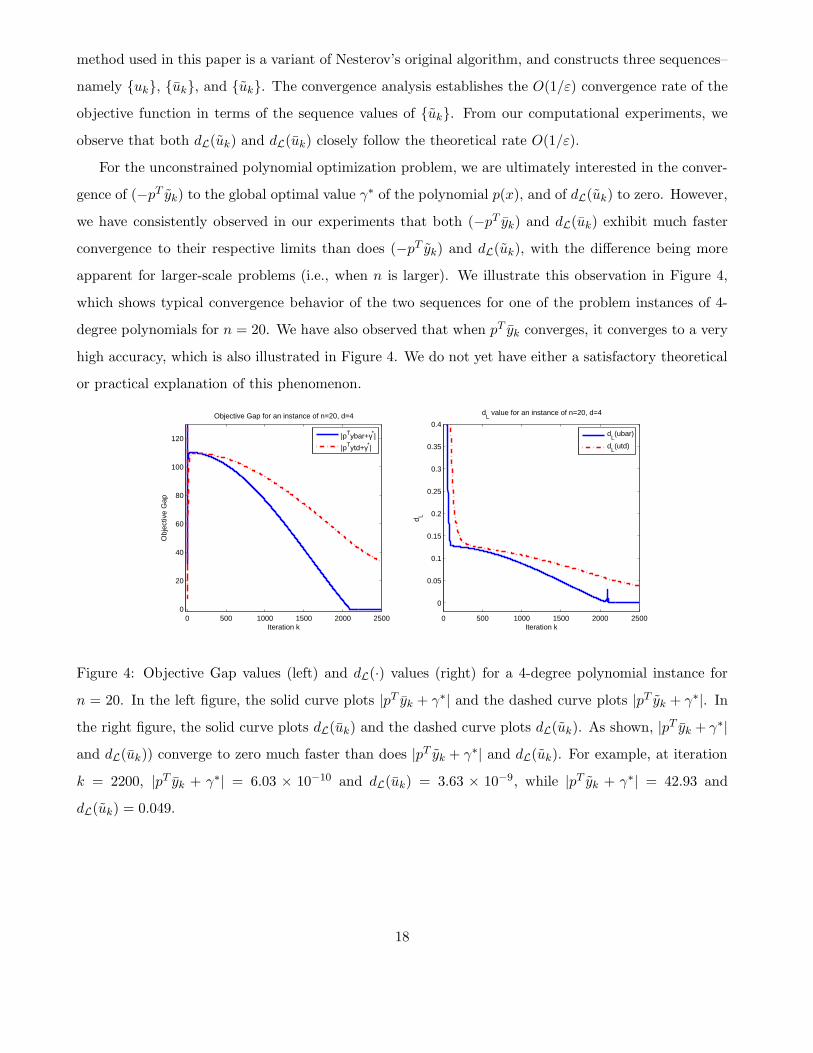
For the unconstrained polynomial optimization problem, we are ultimately interested in the conver-

gence of (−pT yk) to the global optimal value γ∗ of the polynomial p(x), and of dL(uk) to zero. However,

we have consistently observed in our experiments that both (−pT yk) and dL(uk) exhibit much faster

convergence to their respective limits than does (−pT yk) and dL(uk), with the difference being more

apparent for larger-scale problems (i.e., when n is larger). We illustrate this observation in Figure 4,

which shows typical convergence behavior of the two sequences for one of the problem instances of 4-

degree polynomials for n = 20. We have also observed that when pT yk converges, it converges to a very

high accuracy, which is also illustrated in Figure 4. We do not yet have either a satisfactory theoretical

or practical explanation of this phenomenon.

0 500 1000 1500 2000 25000

20

40

60

80

100

120

Iteration k

Obj

ectiv

e G

ap

Objective Gap for an instance of n=20, d=4

|pTybar+γ*|

|pTytd+γ*|

0 500 1000 1500 2000 2500

0

0.05

0.1

0.15

0.2

0.25

0.3

0.35

0.4

Iteration k

d Ld

L value for an instance of n=20, d=4

d

L(ubar)

dL(utd)

Figure 4: Objective Gap values (left) and dL(·) values (right) for a 4-degree polynomial instance for

n = 20. In the left figure, the solid curve plots |pT yk + γ∗| and the dashed curve plots |pT yk + γ∗|. In

the right figure, the solid curve plots dL(uk) and the dashed curve plots dL(uk). As shown, |pT yk + γ∗|and dL(uk)) converge to zero much faster than does |pT yk + γ∗| and dL(uk). For example, at iteration

k = 2200, |pT yk + γ∗| = 6.03 × 10−10 and dL(uk) = 3.63 × 10−9, while |pT yk + γ∗| = 42.93 and

dL(uk) = 0.049.

18

4 Discussion

We have applied an accelerated first-order method to solve unconstrained polynomial optimization

problems. By exploiting special structural properties of the problem, namely the orthogonality of

the moment matrices, the computational cost of the accelerated first-order method is greatly reduced.

Numerical results on degree-4 and degree-6 polynomials demonstrate that the accelerated first-order

method is capable of solving polynomials with at least twice as many variables as existing interior-point

method software (SeDuMi) can handle. We have observed some curious convergence behavior of the

iterate sequences of the accelerated first-order method that does not follow from the usual convergence

analysis of such methods. This observation bears further study.

In the last several years, several researchers have worked on algorithms for solving large-scale SDPs,

see, for example, [18] and [28]. In the recent work of [20], these algorithms were applied to solve

large-scale unconstrained polynomial optimization problems. The main algorithmic framework in these

recent algorithms is the augmented Lagrangian method, where the linear system at each iteration is

solved by a combination of a semismooth Newton method and a conjugate gradient algorithm. The

computational experiments recently reported for applying these methods to polynomial optimization

in [20] are very promising, for instance they solve 4-degree polynomial optimization problems in up to

n = 100 variables with high precision. These methods utilize second-order Hessian information but have

low memory requirements inherited from the conjugate gradient algorithm. However, the augmented

Lagrangian method in general does not have a global convergence rate guarantee; and indeed, the results

in [24] and [28] show global convergence and local convergence rates only under regularity conditions.

In comparison, the accelerated first-order method has virtually no regularity requirement and admits

an explicit global convergence rate. The parameters in the convergence rate can be derived or bounded

a priori in some cases (for instance, if we know that the optimal solution is contained in a given ball).

As a future research direction, it would be very interesting to merge these two types of algorithms, i.e.,

to use an accelerated first-order method in the initial phase to quickly compute solutions that are in a

neighborhood of the optimal solution, and then switch over to a low-memory second-order method to

compute highly accurate solution iterates thereafter.

19

References

[1] A. Auslender and M.Teboulle. Interior gradient and proximal methods for convex and conic opti-

mization. SIAM J. Optim., 16:697–725, 2006.

[2] Amir Beck and Marc Teboulle. A fast iterative shrinkage-thresholding algorithm for linear inverse

problems. SIAM J. Img. Sci., 2:183–202, March 2009.

[3] S. Becker, J. Bobin, and E. J. Cands. Nesta: a fast and accurate first-order method for sparse

recovery. SIAM J. on Imaging Sciences, 4(1):1–39, 2009.

[4] D. Bertsimas and I. Popescu. Optimal inequalities in probability theory: A convex optimization

approach. SIAM Journal on Optimization, 15:780–804, 2004.

[5] D. Bertsimas and J. Sethuraman. Handbook on Semidefinite Programming, volume 27 of Inter-

national Series in Operations Research and Management Science, chapter Moment problems and

semidefinite programming, pages 469–509. Kluwer, 2000.

[6] Alexandre D’aspremont, Onureena Banerjee, and Laurent El Ghaoui. First-order methods for

sparse covariance selection. SIAM J. Matrix Anal. Appl., 30(1):56–66, 2008.

[7] D.Bertsimas and K.Natarajan. A semidefinite optimization approach to the steady-state analysis

of queueing systems. Queueing Systems and Applications, 56(1):27–40, 2007.

[8] D.Henrion and J.B.Lasserre. Gloptipoly: Global optimization over polynomials with matlab and

sedumi. ACM Transactions on Mathematical Software, 29(2):165–194, June 2003.

[9] Z. Lu G. Lan and R.D.C.Monteiro. Primal-dual first-order methods with O(1/ǫ) iteration-

complexity for cone programming. Technical report, School of Industrial and Systems Engineering,

Georgia Institute of Technology, December 2006.

[10] J.-B. Hiriart-Urruty and C. Lemarechal. Convex Analysis and Minimization Algorithms I, volume

305 of Comprehensive Study in Mathematics. Springer-Verlag, New York, 1993.

[11] I.J.Landau. Moments in Mathematics. AMS, Providence, RI, 1987.

[12] F. Jarre and F. Rendl. An augmented primal-dual method for linear conic programs. SIAM Journal

on Optimization, 19(2):808–823, 2008.

20

[13] J.B.Lasserre. Global optimization with polynomials and the problem of moments. SIAM J. Opti-

mization, 11:796–816, 2001.

[14] M.Coste J.Bochnak and M-F.Roy. Real Algebraic Geometry. Springer, 1998.

[15] Z. Lu. Primal-dual first-order methods for a class of cone programming. submitted, 2009.

[16] Zhaosong Lu. Smooth optimization approach for sparse covariance selection. SIAM J. on Opti-

mization, 19:1807–1827, February 2009.

[17] L.Vandenberghe and S.Boyd. Semidefinite programming. SIAM Rev., 38:49–95, 1996.

[18] J. Malick, J. Povh, F. Rendl, and A. Wiegele. Regularization methods for semidefinite program-

ming. SIAM J. Optim., 20(1):336–356, 2009.

[19] M.Laurent. Semidefinite programming in combinatorial and polynomial optimization. NAW,

5/9(4), December 2008.

[20] J. Nie. Regularization methods for sum of squares relaxations in large scale polynomial optimiza-

tion. Technical report, Department of Mathematics, University of California, 9500 Gilman Drive,

La Jolla, CA 92093, 2009.

[21] P. Parrilo. Structured Semidefinite Programs and Semialgebraic Geometry Methods in Robustness

and Optimization. PhD thesis, California Institute of Technology.

[22] P.Parrilo. Semidefinite programming relaxations for semialgebraic problems. Math. Prog., 96(2,

Ser. B):293–320, 2003.

[23] S. Prajna, A. Papachristodoulou, P. Seiler, and P. A. Parrilo. SOSTOOLS: Sum of squares op-

timization toolbox for MATLAB, 2004. Available from http://www.cds.caltech.edu/sostools

and http://www.mit.edu/~parrilo/sostools.

[24] R. T. Rockafellar. Augmented lagrangians and applications of the proximal point algorithm in

convex programming. Math. Oper. Res., 1:97–116, 1976.

[25] J.F. Sturm. Using sedumi 1.02, a matlab toolbox for optimization over symmetric cones. Opti-

mization Methods and Software, (11-12):625–653, 1999. Special issue on Interior Point Methods.

[26] Y.Nesterov. A method for unconstrained convex minimization problem with the rate of convergence

o(1/k2). Doklady, 269:543–547, 1983. translated as Soviet Math. Docl.

21

[27] Y.Nesterov. Introductory Lectures on Convex Optimization: A Basic Course. Kluwer, Boston,

2004.

[28] X. Zhao, D. Sun, and K. Toh. A newton-cg augmented lagrangian method for semidefinite pro-

gramming. SIAM J. Optim., 20(4):1737–1765, 2010.

22