
An Abstract of the Thesis of Douglas J. Geller for the ...
142
An Abstract of the Thesis of Douglas J. Geller for the Master of Science Degree in Physical Sciences (Earth Science with Hydrogeology Emphasis) presented May 2011. Title: An Evaluation of Three Methods for Assessing Long-Term Well Yield Abstract approved: __________________________________________________ Safe yield and sustainable yield are highly relevant topics in the fields of hydrogeology and water management. Most published information on safe yield has focused on aquifer systems, while relatively little attention has been paid to the safe yield of individual wells, termed here the long-term well capacity (LTWC). The little-studied long-term well capacity is typically viewed as a fixed value, although it might change over the life of any production well. To test the hypothesis that methods to estimate LTWC may be more broadly applied, three LTWC estimation methods, all based on the theory of radial flow to wells, are tested in a comparative analysis. The methods are tested along with traditional analytical approaches for interpreting pumping tests to determine both hydraulic properties and LTWC. To gain insights into how individual well capacity may be related to the larger context of groundwater management, pumping test data from ten wells completed in a variety of hydrogeologic settings with yields ranging from 2 gpm to 3,500 gpm are assessed using the three LTWC methods, which allow the analyst to estimate either a 100-day (Q 100d ) or a 20-year (Q 20 ) LTWC. The subject wells, completed in confined, unconfined and fractured bedrock aquifers located in Kansas, Oregon and British Columbia Canada, are analyzed using pressure derivative analysis to determine radial flow conditions, interpreted using conventional pumping test analysis to estimate aquifer properties, and then further
Transcript of An Abstract of the Thesis of Douglas J. Geller for the ...

An Abstract of the Thesis of Douglas J. Geller for the Master of Science Degree in
Physical Sciences (Earth Science with Hydrogeology Emphasis) presented May 2011.
Title: An Evaluation of Three Methods for Assessing Long-Term Well Yield
Abstract approved: __________________________________________________
Safe yield and sustainable yield are highly relevant topics in the fields of
hydrogeology and water management. Most published information on safe yield has
focused on aquifer systems, while relatively little attention has been paid to the safe yield
of individual wells, termed here the long-term well capacity (LTWC). The little-studied
long-term well capacity is typically viewed as a fixed value, although it might change
over the life of any production well.
To test the hypothesis that methods to estimate LTWC may be more broadly
applied, three LTWC estimation methods, all based on the theory of radial flow to wells,
are tested in a comparative analysis. The methods are tested along with traditional
analytical approaches for interpreting pumping tests to determine both hydraulic
properties and LTWC. To gain insights into how individual well capacity may be related
to the larger context of groundwater management, pumping test data from ten wells
completed in a variety of hydrogeologic settings with yields ranging from 2 gpm to 3,500
gpm are assessed using the three LTWC methods, which allow the analyst to estimate
either a 100-day (Q100d) or a 20-year (Q20) LTWC.
The subject wells, completed in confined, unconfined and fractured bedrock
aquifers located in Kansas, Oregon and British Columbia Canada, are analyzed using
pressure derivative analysis to determine radial flow conditions, interpreted using
conventional pumping test analysis to estimate aquifer properties, and then further
evaluated using the three methods. From each set of results ratios of projected long-term
specific capacity to actual measured short-term specific capacity are derived. A
sensitivity analysis performed on the results involved systematically varying pumping
time and a default safety factor applied in each LTWC equation. For two wells completed
in the Ogallala aquifer in Kansas, the effects of aquifer depletion on LTWC are
investigated, and the effects of well interference on two confined aquifer wells in Oregon
are assessed.
The first of the three methods tested (Farvolden) was found to produce the least
reliable results due to the assumption that drawdown during the first minute of pumping
is negligible. This may lead to either an over- or under-estimation of LTWC. The Moell
and CPCN methods were found to produce consistent results. Specific capacity ratios
derived from each calculated data set helped validate results, and showed that four
Farvolden calculations were questionable, projecting a long-term specific capacity that
surpassed the measured or observed value during the test. The specific capacity ratios
also facilitate qualitative assessment of sensitivity to changes in pumping time or safety
factor. For most wells, the results showed similar sensitivity to order-of-magnitude
changes in pumping time or 0.1 adjustment in safety factor, with either adjustment
changing the resulting LTWC value by approximately 15%, although the LTWC values
for the Moell method varied over a wider range when pumping time was varied by an
order of magnitude, with the variation depending on whether the well had a low,
moderate or high specific capacity ratio.
Effects of aquifer depletion in the High Plains / Ogallala aquifer significantly
reduce the LTWC of production wells. This is due to reduced available drawdown
(saturated thickness), and decreased aquifer transmissivity from progressive dewatering
of permeable aquifer materials. Observed declines in two areas of Groundwater
Management District 3 over the past 30 years resulted in an estimated 25 to 30%
reduction in transmissivity, and a corresponding decrease in LTWC ranging from 40 to
75 % in the two wells studied. The assessment suggests that by 2030 one of the wells
studied could have a LTWC value approaching zero.
It is relatively easy to estimate LTWC values for virtually any well subjected to a
pumping test without altering the standard procedure for the pumping test. Such an
approach coupled with a calculation of the applicable specific capacity ratio supplements
the understanding that may be derived from traditional pumping test interpretation.
Pumping test data from the time of original well construction are applicable to
assessments of current or future LTWC using information on groundwater levels, well
specific capacity, pump performance, and other pertinent data.
The evaluation of individual well long-term capacities is recommended when a
water source is of particularly high value and there is a need to understand the long-term
operational characteristics. Such assessment may be of value in supporting water balance
studies in the groundwater systems and the “safe” or “sustainable” yield of aquifers. A
Q20 analysis is probably better-suited to municipal wells or other sources used year-round
on a perennial basis, while a Q100d analysis may be better suited to wells used
intermittently or seasonally for irrigation and other purposes.

AN EVALUATION OF THREE METHODS FOR ASSESSING
LONG-TERM WELL YIELD
________
A Thesis
Presented to
The Departments of Physical Sciences
EMPORIA STATE UNIVERSITY
________
In Partial Fulfillment
of the Requirements for the Degree
Master of Science
________
By
Douglas J. Geller
May 2011

Thesis approved by:
__________________________________
Dr. Marcia Schulmeister, Committee Chair
__________________________________
Dr. James Aber, Committee Member
__________________________________
Dr. Carl McElwee, Committee Member
___________________________________
Dr. DeWayne Backhus, Department Chair
___________________________________
Dr. Kathy Ermler, Dean of the Graduate
School

i
ACKNOWLEDGEMENTS
I conceived of this project while running the trails at Helliwell Provincial Park on
Hornby Island off the British Columbia coast in the summer of 2010. B.C. calls itself the
“most beautiful place on Earth” and it is hard to argue with such a claim when experiencing a
place like Helliwell. When I think back on this project, I know I will fondly recall the Garry
Oaks, the Bald Eagles, and the crags, beaches and trails of Hornby Island.
Many individuals contributed to this project, first and foremost I want to acknowledge
the support and guidance provided throughout by my advisor Dr. Marcia Schulmeister,
Associate Professor of Hydrogeology at Emporia State University, and also thank my
committee members Dr. James Aber, Earth Science Professor at ESU and Dr. Carl McElwee
of Professor Emeritus at Kansas University for their valuable input during thesis preparation.
Appreciation is also extended to my wife Mary Ann, and children, Ethan, Gabe, and Lucas
for putting up with many evening sessions glued to the computer. This work was funded in
part by the Kansas Water Office and Emporia State University and this support is appreciated.
Jeff Binder of Burns and McDonnell engineers and Mike Dealy of KGS provided the
Ogallala well data analyzed herein, and ESU Earth Science student Sarah Pick assisted with
some of the spreadsheet data entry for the Ogallala wells.
Lastly, a word of thanks is extended to Dr. Garth van der Kamp of the National Water
Research Institute of Environment Canada, who provided copies of the publications he co-
authored that are cited herein, and whose work provided some of the impetus for pursuing
this research study.

ii
NOTES ON UNITS OF MEASUREMENT
The water well industry in North America continues to use imperial units of
measurement, such as gallons per minute (gpm), feet (ft), and so on. The original data used
in this study were also measured and recorded in these units. Therefore, imperial units of
measurement are used throughout. Selected conversions from U.S. imperial to metric units of
measurement appear in the table below.
Value U.S. imperial units Metric equivalent
Flow rate Gallons per minute (gpm) 1 gpm = 3.78 liters per minute
Flow rate Gallons per minute (gpm) 1 gpm = 5.4 m3/day
Distance Inches (in) 1 in = 2.54 cm
Distance or depth Feet (ft) 1 ft = 30 cm
Distance or depth Feet (ft) 1,000 ft = 305 m
Distance Miles (mi) 1 mi = 1,610 m (1.6 km)
Aquifer transmissivity Gallons-per-day per ft (gpd/ft)
1 gpd/ft = 1.2 E-02 m2/day
Aquifer transmissivity Square-feet per day (ft2/day)
1 ft2/day = 9.2 E-02 m2/day
Hydraulic conductivity Feet per day (ft/day) 1 ft/day = 30 cm/day = 3.6E-06 m/sec
Notes: cm = centimeters; m = meters; m3 = cubic meters; km = kilometer; m = minute only when used in gpm
iii
TABLE OF CONTENTS
ACKNOWLEDGEMENTS ....................................................................................................... i
NOTES ON UNITS OF MEASUREMENT ............................................................................. ii
TABLE OF CONTENTS ......................................................................................................... iii
LIST OF APPENDICES ........................................................................................................... v
LIST OF TABLES ................................................................................................................... vi
LIST OF FIGURES ................................................................................................................ vii
CHAPTER 1 INTRODUCTION ............................................................................................. 1 1.1 Well and Aquifer Yield Concepts and Definitions .................................................. 3 1.2 Problem Statement and Study Objectives .............................................................. 10
CHAPTER 2 AQUIFER AND PUMPING TEST OVERVIEW AND CONCEPTS ............ 12 2.1 Purposes of Pumping Tests .................................................................................... 12 2.2 Analytical Methods to Determine Hydraulic Properties ........................................ 14
2.2.1 Theis method of curve-matching ........................................................................ 15 2.2.2 Cooper-Jacob straight-line method ..................................................................... 17 2.2.3 Unconfined aquifers – delayed yield and surface water recharge effects ........... 19 2.2.4 Linear and fracture flow models ......................................................................... 21 2.2.5 Pressure derivative analysis ................................................................................ 23 2.2.6 Step pumping tests .............................................................................................. 27
CHAPTER 3 PREVIOUS WORK ON WELL YIELD DETERMINATION METHODS .. 31 3.1 Quantitative Methods Based on Radial Flow Theory ............................................ 32
3.1.1 Theoretical background to the quantitative methods .......................................... 32 3.1.2 Method “A”: Farvolden (1959) ......................................................................... 38 3.1.3 Method “B”: Moell (1975) ................................................................................. 40 3.1.4 Method “C”: B.C. Ministry of Environment (1999) .......................................... 40 3.1.5 Modified Moell method of Maathuis and van der Kamp (2006) ........................ 42
3.2 Other Methods ........................................................................................................ 44 3.2.1 Pumping test analytical simulation ..................................................................... 44 3.2.2 Flow modeling .................................................................................................... 45 3.2.3 Volumetric and other pumping test-based methods ............................................ 46 3.2.4 Equilibrium (stabilized drawdown) .................................................................... 49
CHAPTER 4 DATA SOURCES AND METHODOLOGY .................................................. 50 4.1 Description of Pumping Test Data Sets and Test Conditions ................................. 50
4.1.1 Criteria for and process of selecting pumping test data sets ............................... 50 4.1.2 Description of test well data ............................................................................... 52 4.1.3 Pumping test and data collection procedures ...................................................... 54 4.1.4 Data set summaries ............................................................................................. 63
4.2 Data Processing and Analysis Methods .................................................................. 76 4.2.1 Specific capacity ratios ....................................................................................... 77 4.2.2 Sensitivity analysis .............................................................................................. 79
CHAPTER 5 RESULTS ........................................................................................................ 81

iv
5.1 Pumping Test Interpretation ................................................................................... 81 5.2 Long Term Well Capacity Results .......................................................................... 82 5.3 Sensitivity Analysis Results .................................................................................... 86
5.3.1 Method A Farvolden sensitivity .......................................................................... 86 5.3.2 Method B Moell method sensitivity results ........................................................ 89 5.3.3 Method C CPCN sensitivity results .................................................................... 92
5.4 Summary ................................................................................................................. 94
CHAPTER 6 DISCUSSION ON SELECTED TECHNICAL ISSUES ............................... 97 6.1 Well Construction Factors Influencing Long Term Capacity ................................ 97 6.2 Seasonal or Annual Water Level fluctuation ......................................................... 99 6.3 Factoring in Changes in Well Performance (Specific Capacity) ........................... 99 6.4 Pump Performance Considerations ........................................................................ 99 6.5 Investigation of Well Interference Effects ........................................................... 100 6.6 Investigation of Long Term Mining Yield ........................................................... 102
6.6.1 LTMY of UC3 and UC4 using current HA ....................................................... 103 6.6.2 Effect of reduced aquifer transmissivity on long-term well capacity ............... 105
6.7 Use of Analytical and Numerical Models ............................................................ 113
CHAPTER 7 CONCLUSIONS .......................................................................................... 115 7.1 Findings on the Q20 Methods A and B of Farvolden and Moell .......................... 115 7.2 Findings on the Q100d Method C (CPCN) ............................................................ 117 7.3 Implications for Groundwater Management ........................................................ 117
7.3.1 Municipal and other semi-continuously used wells ........................................... 118 7.3.2 Irrigation and other seasonally used wells ......................................................... 118 7.3.3 Wells in groundwater decline situations based on the Ogallala case ................. 119
7.4 Opportunities for further research ........................................................................ 120
REFERENCES ..................................................................................................................... 123

v
LIST APPENDICES
Appendix A Well test data worksheets and interpreted hydrographs…………………….130
Appendix B Well capacity calculation worksheets and sensitivity analysis results…….. 201
Appendix C Well construction information………………………………………………211

vi
LIST OF TABLES
Table 4.1. Well construction summary ................................................................................ 57
Table 4.2 Pumping test summaries ..................................................................................... 76
Table 5.1 Aquifer Test Interpretation Summary ................................................................. 82
Table 5.2 Method A (Farvolden) well capacity estimation results ..................................... 83
Table 5.3 Method B (Moell) well capacity estimation results ............................................ 84
Table 5.4 Method C (CPCN) well capacity estimation results ........................................... 84
Table 5.5 Comparison of all methodologies results ............................................................ 85
Table 6.1 Analysis of Wells CF1 and CF2 well interference effects ................................ 102
Table 6.2 Estimated long-term mining yield of High Plains / Ogallala wells UC3 and UC4 .......................................................................................................................... 103

vii
LIST OF FIGURES
Figure 2.1 Characteristic Theis type time-drawdown response curve generated with the software program AqtesolvTM ......................................................................... 18
Figure 2.2 Typical semi-log straight line plot of drawdown versus log of time .............. 19
Figure 2.3 Hydrograph of a well exhibiting a strong surface water recharge effect ........ 22
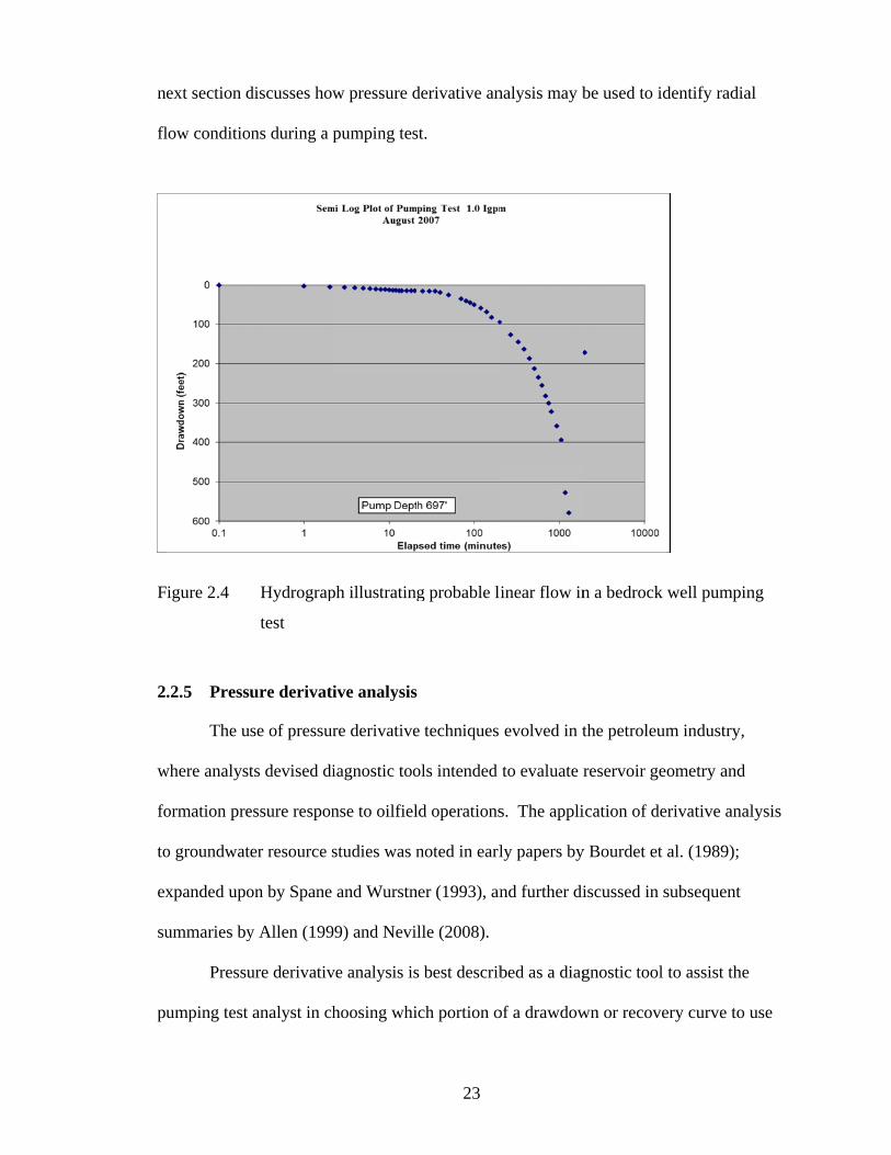
Figure 2.4 Hydrograph illustrating probable linear flow in a bedrock well pumping test 23
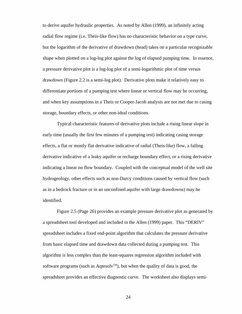
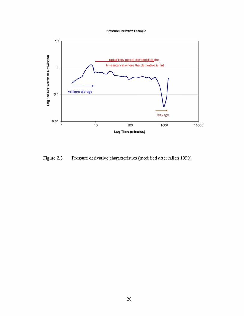
Figure 2.5 Pressure derivative characteristics (modified after Allen 1999) ..................... 26
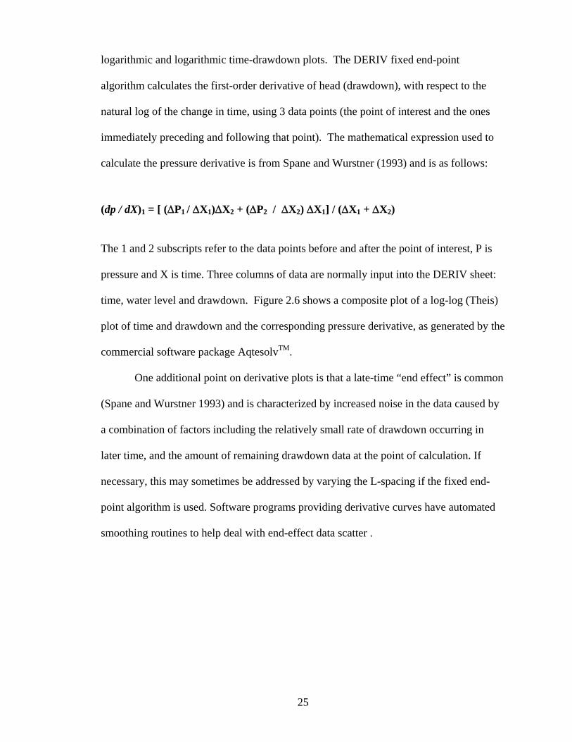
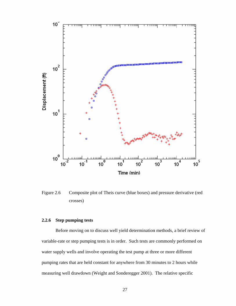
Figure 2.6 Composite plot of Theis curve (blue boxes) and pressure derivative (red crosses)........................................................................................................... 27
Figure 2.7 Example step test s/Q versus Q plot and laminar head loss calculation ......... 30
Figure 3.1 Semi-logarithmic plot of time on log scale and water level or drawdown on linear (y axis) scale .......................................................................................... 35
Figure 3.2 Semi-logarithmic plots showing S and HA values, and a straight-line drawdown projection ....................................................................................... 37
Figure 4.1 General location of field sites in Oregon, British Columbia, and Kansas ...... 51
Figure 4.2 Typical test well configuration showing well sounder, sounding tube (red arrow), sampling tap (A), control valve (B) .................................................... 58
Figure 4.3 Test pumping well head with well sounder (A), flow meter (B) and control valve (C) .......................................................................................................... 59
Figure 4.4 Flow measurement using circular orifice plate and manometer ..................... 60
Figure 4.5 Typical High Plains / Ogallala aquifer irrigation well, Scott County, KS ...... 61
Figure 4.6 Preparing submersible test pump for installation. Note dual PVC sounding tubes (arrow).................................................................................................... 62
Figure 4.7 General location of Ogallala wells UC3 and UC4 .......................................... 73
Figure 5.1 Method A time-of-pumping sensitivity graphs ............................................... 88
Figure 5.2 Method A Q20 safety factor sensitivity graph for CF1 .................................... 89
Figure 5.3 Method B time of pumping sensitivity graphs ................................................ 91
Figure 5.4 Method B Q20 safety factor sensitivity graph for CF1 and UC1 ..................... 92
Figure 5.5 Method C time of pumping sensitivity graphs ................................................ 94
Figure 6.1 Hydrograph of Annual Water Level Well T24S, R33W, 34CAC ................ 104
Figure 6.2 Hydrograph of Annual Water Level Well T28S, R21W, 23DBC ................ 105
Figure 6.3 Base case (1979) predicted drawdown curve for UC3 ................................. 108
Figure 6.4 Year 2010 predicted drawdown response for UC3 ....................................... 109
Figure 6.5 Base-case (1977) predicted drawdown curve for UC4 ................................. 110

viii
Figure 6.6 Year 2010 predicted drawdown curve for UC4 ............................................ 111
1
CHAPTER 1
INTRODUCTION
Well yield is the measured volume of water produced per a unit of time (Driscoll
1986), usually expressed as gallons per minute (gpm). While the instantaneous discharge
rate from a well can be readily measured, the determination of a reasonable or “safe” rate
of production over the long-term is not so straightforward. Just as the discharge of a
surface stream may vary over time, the same is true for groundwater well production, and
yet water managers and the public at large tend to view well yield as a fixed value.
Further complicating matters is the fact that there is no broadly applied or universally
accepted approach within the field of hydrogeology to quantitatively estimate long-term
well yield. Sophocleous (2000) noted that concepts of well yield, aquifer “safe yield”
and “sustainable yield” have different meanings but are sometimes used interchangeably,
and without sufficient context.
Just as there has historically been more published literature on aquifer hydraulics
than papers focused on well hydraulics (Williams 1981), the literature on methods to
quantitatively determine the yield of individual wells is sparse when compared to those
assessing the safe or sustainable yield of an aquifer system, or a connected groundwater-
surface water system.
The ultimate yield of an aquifer or aquifer system depends on several fixed and
variable factors, including; the amount of water in storage, how readily water is
transmitted through the aquifer pore spaces, the natural water input and output processes,
the location, frequency, the location, duration and magnitude of groundwater pumping,
and the effects that pumping has on the pre-development aquifer’s state of dynamic
equilibrium (groundwater balance).

2
In turn, the long term yield of an individual well is governed by the hydraulic
properties of the well, how it was constructed, the duration of pumping, as well as the
hydraulic and hydrodynamic properties of the aquifer. Thus a seemingly simple question
such as “how much water should I count on from this well”, while reasonable enough, is
exceedingly difficult to answer, especially at the time of initial well installation when key
regulatory and operational decisions about a well’s long-term use are typically made.
Maathuis and van der Kamp (2006) point out that the consequences of
groundwater development are rarely predicted reliably, and only become apparent
following a considerable period of time (usually years, or decades). And yet, there is a
need to quantify an individual well’s yield for many reasons that are of immediate
concern, such as choosing a well pump, planning for other wells, and assessing near-term
impacts that may be caused by or inflicted upon a new groundwater source. Therefore, it
follows that a sound approach to assessing an individual well yield forms an important
step in the process of understanding how wells, and the aquifer in which they are
completed, respond to long term groundwater withdrawals.
Concepts of aquifer “safe yield” and “sustainability” in groundwater resource
management have been active discussion and research topics in the recent literature (e.g.
Sophocleous [2000], Kendy [2003], Kalf and Wooley [2005]). Recognizing that the
question of individual well yield has received less attention in the literature, and
application of methodologies has been quite limited, this study intends to bridge gaps
between the concepts of aquifer safe yield, sustainable groundwater development, and the
long-term production capacity of individual wells (or yield). The goal of this thesis is to
develop a framework for broader application of quantitative methods to estimate long-

3
term well capacity (LTWC), and to provide recommendations for use of these methods in
groundwater management. The two-part hypothesis to be tested in this study comprises
the following:
1. That promising and yet under-utilized methods to assess LTWC could be applied
more broadly and beyond the localities where they were first developed; and
2. By subjecting each method to a quantitative comparative analysis involving
multiple data sets, the relative strengths, weaknesses and applicability of each
method might be better understood.
To test the hypothesis that these methods could be applied more broadly than they
are at present, the research compares three promising but understudied methods used to
estimate the long-term capacity of individual pumping wells. LTWC predicted by the
three methods were determined in multiple aquifer types based on eleven (11) sets of
pumping test data from ten (10) wells. The results are evaluated in a discussion of the
methods used for management of wells and aquifer systems for safe or sustainable yield.
This first chapter introduces important concepts and definitions, outlines the research
problem, and the study objectives.
1.1 WELL AND AQUIFER YIELD CONCEPTS AND DEFINITIONS
Within the practice of hydrogeology, the concept of safe yield has been in use
since the early 1900s (Lee 1915) and in common use since about the mid-1900s (Baker
1955), while the key concepts began to be explored by Theis (1940) in what remains a
vital contribution on the topic, titled “The source of water derived from wells.” Other
terms such as Safe Well Yield, Safe Aquifer Yield, Sustainable Yield, and Long-Term Well
Capacity have also been introduced and used in the literature and in general practice.
These terms attempt to describe and quantify values that are only be approximated or
4
estimated with what is usually a considerable degree of uncertainty. As noted by
Maathuis and van der Kamp (2006), because the long term response of aquifer systems to
groundwater development is difficult to predict, the effects of withdrawal should be
monitored, identified and dealt with as pumping proceeds. This statement is also true for
individual wells within an aquifer system.
Despite the theoretical limitations in doing so, it remains a practical necessity to
make predictions of well yield, and such assessments form a basis for water management
decisions that have far-reaching implications. A U.S.G.S. report on a sustainable yield
estimation tool for the state of Massachusetts (Archfield et al. 2009) noted that the “safe
yield” term as it is most often used in water resource management typically implies that a
single fixed value represents the water available for withdrawal given some singular
limiting factor (or constraint), such as a predicted drought recurrence or (for surface
water) a minimum instream flow threshold.
The following are a few definitions of the various safe yield terms, adapted from a
number of sources including Driscoll (1986), Sophocleous (1998), Fetter (2001), Rivera
(2006), Maathuis and van der Kamp (2006), and proposed for use in this study.
Well Yield (WY): Generally, well yield is defined as the flow rate that can be maintained
over a given time period, such as gallons per minute (gpm). In practice, well yield may
be estimated by a well driller or measured during a pumping test.
Safe Well Yield (SWY): While well yield is a measured flow rate, safe well yield is an
estimated value and is the volume (or rate) of water that can reliably be produced by an
individual well for a pre-determined length of time, usually based on one or more defined
constraints. Typical safe well yield time factors range from 1 day to 20 years. SWY will
be termed herein as the Long-Term Well Capacity (LTWC), so as to specifically avoid
5
using the term “Safe.” This convention thus makes a clear distinction between individual
well capacity and aquifer system safe yield. The LTWC value may be calculated
independently of any water-budget analysis or modeling; but should be a value that is less
than the following two terms, if they are estimated. As noted by Rivera (2006), SWY is
more of a local-scale concept determined primarily on the basis of a pumping test, with
uncertainty addressed through the use of safety factors (see page 7) and other adjustments
to the well yield.
Safe Aquifer Yield (SAY): This is the volume of water than can theoretically be removed
from an aquifer based on the water budget. The water budget is the summation of all
inputs to and outputs from the aquifer. The budget is usually derived from a combination
of measured and estimated values, such as climate and runoff data, measured or estimated
evapotranspiration, with the groundwater recharge calculated as a residual in the water
balance equation. The water budget may also be expanded and refined by incorporating
terms such as artificial recharge, groundwater pumping, irrigation return flow, inflow
from adjacent aquifers and so on. Based on a water budget, SAY is commonly thought of
as equal to groundwater recharge or discharge, although Sophocleous (2000) and others
have noted that safe aquifer yield cannot be equal to the recharge (see further discussion
below). As noted by Fetter (2001), over the years, the SAY definition has been modified
by adding qualifiers such as:
The amount of water that can be pumped regularly and permanently without
dangerous depletion of the storage reserve (Lee 1915);
The amount of water that can be pumped economically (Meinzer 1923); and
The amount of water that can be pumped without causing undesirable water
quantity or quality changes (Todd 1959).
6
A composite “modern” definition, from Alley et al. (1999) and Fetter (2001) is
that SAY is the amount of naturally-occurring groundwater that can be withdrawn from
an aquifer on a sustained basis, economically and legally, without impairing the native
groundwater quality or creating an undesirable effect, such as land subsidence, or drying
up of wetlands or other groundwater-dependent ecosystems. [It is worth noting that this
SAY definition is what Sophocleous (2000) would probably consider to represent
Sustainable Yield].
Regardless of the exact terminology used (safe or sustainable), there is relative
consensus in recent literature that SAY is best represented conceptually as a percentage
of the natural groundwater discharge (or a combination of discharge and induced
recharge) that can be effectively captured (by wells) without causing undesirable effects.
This percentage is not fixed in space or time, and should be governed by what and who
are dependent on continued discharge from the aquifer system, and what economic,
societal and environmental values are placed on continuation of such discharge. In parts
of Australia, a default value of 30% of natural groundwater discharge may be captured
and assumed to be safe (or sustainable), until proven otherwise in detailed studies (Kalf
and Woolley, 2005).
Sustainable Groundwater Yield (SGY): The volume of water than can be removed from
the aquifer based on the water budget, including water that must be reserved for
ecological or other non-consumptive purposes.
Sustainable Development (SD): This is a regional-scale concept for a whole aquifer
system, including interconnected stream-aquifer systems and groundwater-dependent
ecosystems functioning in a watershed.

7
Safety Factor (Sf): Methods to determine LTWC may include a safety factor in the
equation. The safety factor reduces the calculated LTWC value by an arbitrary amount,
and is a means to account for natural variation in groundwater systems and/or
uncertainties in the data analysis. The safety factor is explained further in Chapter 4.
The concepts of safe aquifer yield, and sustainable yield, in general, have been
widely debated and discussed in the literature. An early cited reference to the concept of
safe yield is the paper by Lee (1915). In a recent commentary, Keddy (2003) highlighted
how the fundamental safe yield concepts, first introduced by Theis in 1940, have been
actively reiterated and expanded upon by Bredehoeft et al. (1982), Bredehoeft (1997;
2002), Sophocleous (1997), and Alley et al. (1999), to name a few of the better-known
papers. Many of these writers note how the simplification of safe yield concepts led to a
practice, by some hydrogeologists, of determining safe yield on the basis of a water
budget where the natural groundwater recharge rate is estimated, usually as a residual in a
general water balance equation, and then this recharge rate is taken to be the upper safe
limit of groundwater development. This approach fails because it ignores the fact that
without inflow from recharge, natural or artificial groundwater discharge ultimately
depletes the resource. Pumping up to 100% of the recharge reduces discharge to surface
water, which has environmental consequences.
Lohman (1972) noted that the term “safe yield” has many definitions, as many
have attempted to define it, and also noted that it is questionable as to who should
determine safe yield (however it is defined) – hydrogeologists or those who manage a
groundwater resource. Lohman settled on a definition that is easy for anyone to
understand: “The amount of groundwater one can withdraw without getting into trouble”
(p. 62).
8
The core of these literature “discussions” on what has been variously described as
the “elusive" concept of safe yield (Sophocleous 1998) or the “paradox” of safe yield
(Fetter 2001) is that prior to any groundwater development, there is a natural water
balance such that recharge is equal to natural discharge (plus or minus any natural change
in groundwater storage). Bredehoeft, Papadopolus and Cooper’s “Water Budget Myth”
paper (Bredehoeft et al. 1982) argued that the common practice of estimating the natural
recharge rate and setting this as the limit of safe yield is not scientifically correct, going
on to point out that the natural recharge rate is in fact irrelevant to the question of safe
yield. Deconstructing the safe yield myth further, Alley et al. (1999) pointed out that the
total pumping rate is also irrelevant, arguing that the net groundwater extraction (after
correcting for return flows) must be differentiated in any detailed water balance analysis,
as only the actual consumption should be included in the water balance equation.
Theis (1940) was the first to point out that any groundwater pumping must be
balanced by one or more of the following:
An increase in the recharge rate;
A decrease in the natural discharge rate; and/or
A reduction of water stored in the aquifer.
The above concepts were thoroughly reiterated later by Alley et al. (1999), Sophocleous
(2000), and others. Theis (1940) also introduced the concept of “capture”, which is the
water derived from the combined decrease in natural (undeveloped) discharge and the
increase in (undeveloped) recharge (Bredehoeft and Durbin 2009). Pumping that exceeds
the system’s capture capability destabilizes the system, and results in groundwater level
declines.
9
The Okanagan Basin Water Board (OBWB 2009) in western Canada completed a
basin-scale surface and groundwater balance study and model. This study incorporated
the results of a detailed groundwater balance analysis that differentiated net consumptive
groundwater use from return flows. This is but one of many examples of how these
principles are now being applied. An annual water budget for a given land area of
interest used in the OBWB (2009) study comprises the following terms:
P = SR + AET + GWR
where
P = average annual precipitation
SR = average annual surface runoff
AET = average annual actual evapotranspiration
GWR = average annual groundwater recharge
Long-term mining yield: Sophocleous (1998) also proposed a term for non-sustainable
groundwater yield, termed the mining yield. This is the amount of water that can
realistically be withdrawn from an aquifer that is in decline, such as is the case with parts
of the High Plains Aquifer in western Kansas and other nearby states. This could take the
form of planned or unplanned depletion. Projected groundwater level declines brought on
by the progressive removal of groundwater in storage means that at some point in the
future, if declines continue unmitigated, that aquifer or well yield approaches a null
value. Decline in water levels impacts the yield of individual wells due to the loss of
available drawdown and transmissivity. This has already been observed in irrigated
agricultural regions reliant upon the High PlainsAquifer, including the portion of this
aquifer system hosted in the Ogallala Formation in western Kansas, herein termed the
Ogallala aquifer. Large groundwater level declines due to heavy pumping have reduced
saturated thickness in some areas to the extent that farmers have abandoned their wells

10
(Groundwater Management District 3 2004). This study describes a predicted future well
capacity based on forecasted decline rates as the Long Term Mining Yield (LTMY).
Other key concepts specific to aquifer and well pumping tests, including well test
variables and abbreviations are introduced and defined in Chapter 2.
1.2 PROBLEM STATEMENT AND STUDY OBJECTIVES
As already noted, the topic of individual well safe yield (termed here long-term
well capacity) has not been studied as much as the yield of aquifer systems through
investigations of the “groundwater budget” and “safe yield.” This study proposes that
methods to estimate LTWC could be applied more broadly without altering the procedure
for conducting a well pumping test and the ensuing data analysis. As a practical matter,
most well pumping tests are of relatively short duration, and extract a smaller volume of
water from the aquifer system being developed relative to the probable long-term
withdrawal pattern. This requires pumping test data to be extrapolated, an exercise that is
fraught with uncertainty (van der Kamp and Maathuis 2005). The problem of
extrapolation is not unique to pumping test analysis, it is of fundamental concern to many
groundwater studies, for example, in groundwater flow modeling (Anderson and
Woessner 1992).
A thorough understanding of the assumptions, advantages and shortcomings of
the various methods used to derive long-term well capacity estimates supports ongoing
groundwater management and aquifer yield research. Furthermore, a more systematic
approach to deriving well capacity from pumping test data contributes to more confident
predictions of the groundwater extraction component of a water budget, and also allow
for comparisons between predicted yield and actual groundwater usage. This is achieved
by completing the following steps:
11
1. Compile and test a number of existing methods that are used to estimate long-term
well capacity. Select quantitative methods for evaluation and testing.
2. Compare the methods by utilizing multiple data sets derived from controlled
pumping tests on wells of varying depth and yield, and representing a variety of
hydrogeologic settings.
3. Assess the temporal sensitivity of each method to different assumed pumping
durations and whether results are sensitive to changes in other variables, for
example safety factors.
4. For the test scenarios evaluated, draw out the relationships between individual
well yield (capacity) and aquifer capacity and the implications for groundwater
management. Investigate the implications of issues such as well interference, and
groundwater level decline.
5. Determine if an adapted version of one or more of the long-term yield estimation
methods evaluated would be valid for use in broader groundwater resource
evaluation applications and how application of the methods ties in with
groundwater resource management.
6. Provide the theoretical and empirical basis for the recommended methodology,
and identify areas for further research.
Of the various methods known to be applied in North America to estimate the
long-term capacity of individual wells, three were found to be promising and selected for
detailed investigation involving a quantitative analysis using eleven pumping test data
sets. These are the methods of Farvolden (1959), Moell (1975) and B.C. Ministry of
Environment (CPCN; 1999) herein referred to as Methods A, B and C. These methods,
while established, are under-utilized beyond the localities where they were developed,
and in need of further study.
12
CHAPTER 2
AQUIFER AND PUMPING TEST OVERVIEW AND CONCEPTS
This chapter provides an overview of aquifer and well pumping tests starting with
a discussion on the many purposes of pumping tests, and followed by a review of
important analytical methods applied to pumping test data in order to determine aquifer
and well properties. In any evaluation of well yield, it is necessary to have a solid
understanding of aquifer properties and the conceptual hydrogeologic model. It is only
with such understanding that the data derived from a pumping test may be used with
confidence to predict future well performance and yield.
2.1 PURPOSES OF PUMPING TESTS
Numerous texts and papers, for example, Walton (1970), Stallman (1976), Freeze
and Cherry (1979), Driscoll (1986), Fetter (2001), Weight and Sonderegger (2001), and
Neville (2008) describe the many purposes of pumping tests, and speak to the importance
of pumping tests to the practice of hydrogeology in general.
A recent technical commentary in the journal Ground Water by Butler (2009)
reviewed the long-standing practice of conducting pumping tests in water supply and
contaminated site investigations. While confirming the validity of pumping tests as a tool
in water supply studies, Butler pointed out that hydrogeologists should be aware of the
limitations of conventional pumping test approaches that yield bulk or averaged aquifer
property values, especially in regard to contaminant site characterizations, where high-
resolution information (both spatial and temporal) on aquifer properties and contaminant
concentrations is often required. Such techniques have evolved in the past 10 years to
include investigative approaches that may incorporate the use of direct-push technology
(McCall et al. 2002; Schulmeister et al. 2003; Schulmeister et al. 2004). However, for

13
evaluating water supply wells, the constant rate pumping test combined with the variable
rate step test (with and without observation wells), remains the method of choice by most
hydrogeologists, although high-resolution direct-push techniques hold considerable
promise for use in solving site-specific groundwater supply problems, especially in
highly stratified heterogeneous formations.
The hydraulic testing of wells forms an essential component of the hydrogeologic
evaluation process (Weight and Sonderegger 2001), and enables assessment of
groundwater supplies, wellhead protection areas, and groundwater remediation measures
at contaminated sites. The purpose of a pumping test conducted on a water supply well
may include one of more of the following:
To provide insight into well performance such as specific capacity or well
efficiency so that a properly-sized pump may be chosen;
To enable aquifer hydraulic properties to be calculated;
To provide a means to collect and analyze groundwater samples to assess general
water quality, or geochemical changes in water quality due to pumping;
To fulfill a regulatory requirement for completion of a well or reporting of well
yield;
To provide an indication of the potential yield of a well or a group of wells in an
aquifer; to assess the effect of pumping on other wells and/or surface water;
To assess the hydraulic response or connectivity of different hydrogeologic units,
or relationships between groundwater and surface water; and
To provide a calibration data set used in the development and testing of a
groundwater flow model.
14
Depending on the situation, the specific objectives of a pumping test govern the
design and implementation of the testing program. For example, a test with a primary
purpose focused on “proving up” the short-term yield of a well so that an appropriate
pump size can be supplied, is likely to be different from a test conducted in order to
assess well-to-well interference, or to assess suspected aquifer boundaries located at
considerable distances from the pumping well. We are concerned here primarily with
“well tests”- i.e. those pumping tests carried out in order to assess an individual well’s
hydraulic capacity (its yield), although certain external factors affecting well capacity are
addressed later (in Chapter 6). While the use of observation well arrays and multiple-
well pumping tests provide further (and often critically important) insights into the
question of well hydraulic capacity as well as aquifer hydraulic and geometric properties,
the analytical approaches applied to observation well data are not discussed in detail, as
the scope of this study focuses on single pumping well analytical approaches. The use of
analytical and numerical modeling tools to adjust long-term well capacity estimates to
account for well interference is discussed in Chapter 6.
2.2 ANALYTICAL METHODS TO DETERMINE HYDRAULIC PROPERTIES
The process of designing, carrying out and interpreting pumping tests (especially
by hydrogeologists) should ideally be grounded in a conceptual understanding (i.e. a
conceptual model) of how the well and the aquifer in which it is completed responds to
pumping over the long term (Weight and Sonderegger 2001). Although by no means an
exhaustive review of aquifer / pumping test analytical approaches, this section presents
some of the important concepts and reviews the most common analytical approaches used
to interpret pumping tests. In addition to the original scientific publications cited here,

15
useful summaries may be found in Driscoll (1986), Kruseman and de Ridder (1990),
Allen (1999), Neville (2008), and Maathuis and van der Kamp (2006), to name a few.
When there is no change in drawdown with respect to time after a sufficient
amount of time has passed in a pumping test, this constitutes an equilibrium or steady-
state condition. True equilibrium (steady-state) conditions are rarely encountered in
pumping tests and consequently are not covered here in any detail. Although not
reviewed here, useful summaries of equilibrium analytical methods including those of
Theim (1906) and constant drawdown analysis (Jacob and Lohman 1952) may be found
in Lohman (1972) and in Kruseman and de Ridder (1990).
Most pumping tests are of the non-steady state type, which means drawdown
continues to increase (sometimes quite slowly) until the end of the test. Probably the two
most widely-used methods to analyze non-steady, radial flow to a pumping well in a
confined aquifer are those of Theis (1935) and Cooper and Jacob (1946). Through
careful diagnosis of the pumping test response augmented by pressure derivative analysis,
these methods may also be used for certain portions of pumping tests performed on wells
completed in other types of aquifers, including fractured bedrock and unconfined
systems.
Selected other analytical approaches for interpreting non-steady flow to wells are
reviewed briefly, including models for linear and fracture flow, variable-rate (step) test
analysis, and unconfined aquifer response.
2.2.1 Theis method of curve-matching
Theis’ 1935 paper forms much of the basis for today’s understanding of non-
steady radial flow to wells. The hydrogeologic conceptual model on which this analytical

16
approach is based makes the following major assumptions about the tested aquifer and
the pumping test:
Aquifer assumptions:
confined and of a large areal extent;
isotropic and homogeneous, and of constant thickness;
overlain by a low-permeability confining layer, which in turn is overlain
by a water-table (unconfined) aquifer;
the confining layer is impermeable and has a specific storage of zero; and
all water removed from the aquifer is derived from storage.
Pumping test assumptions:
The well has an infinitesimal diameter and fully penetrates the aquifer;
Flow rate is constant;
The only water level (head) changes measured are due to the subject
pumping well;
There are no inertial effects occurring in the wellbore; and
Head in the aquifer remains above the stratigraphic top of the aquifer.
As noted by Neville (2008), the Theis solution and its underlying assumptions are
highly idealized and rarely observed in the field. However, with proper interpretation,
some parts of many well pumping test response data may be analyzed with this method.
Because the Theis method is so widely used and well-known, it provides a useful
“benchmark” (Neville, 2008, Ch. 2, p. 3) against which other conceptual and analytical
models may be compared. The basic Theis formula for determining transmissivity is
given as follows:
17
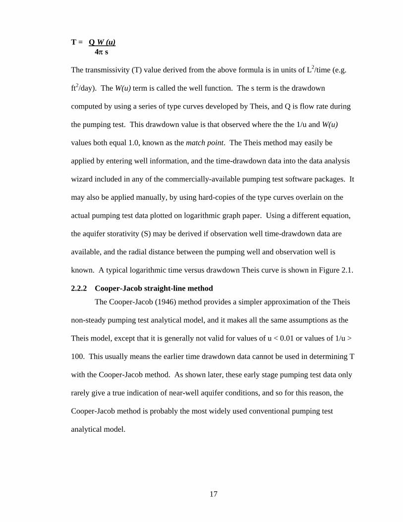
T = Q W (u) 4s The transmissivity (T) value derived from the above formula is in units of L2/time (e.g.
ft2/day). The W(u) term is called the well function. The s term is the drawdown
computed by using a series of type curves developed by Theis, and Q is flow rate during
the pumping test. This drawdown value is that observed where the the 1/u and W(u)
values both equal 1.0, known as the match point. The Theis method may easily be
applied by entering well information, and the time-drawdown data into the data analysis
wizard included in any of the commercially-available pumping test software packages. It
may also be applied manually, by using hard-copies of the type curves overlain on the
actual pumping test data plotted on logarithmic graph paper. Using a different equation,
the aquifer storativity (S) may be derived if observation well time-drawdown data are
available, and the radial distance between the pumping well and observation well is
known. A typical logarithmic time versus drawdown Theis curve is shown in Figure 2.1.
2.2.2 Cooper-Jacob straight-line method
The Cooper-Jacob (1946) method provides a simpler approximation of the Theis
non-steady pumping test analytical model, and it makes all the same assumptions as the
Theis model, except that it is generally not valid for values of u < 0.01 or values of 1/u >
100. This usually means the earlier time drawdown data cannot be used in determining T
with the Cooper-Jacob method. As shown later, these early stage pumping test data only
rarely give a true indication of near-well aquifer conditions, and so for this reason, the
Cooper-Jacob method is probably the most widely used conventional pumping test
analytical model.
F
ar
If
li
tr
T
W
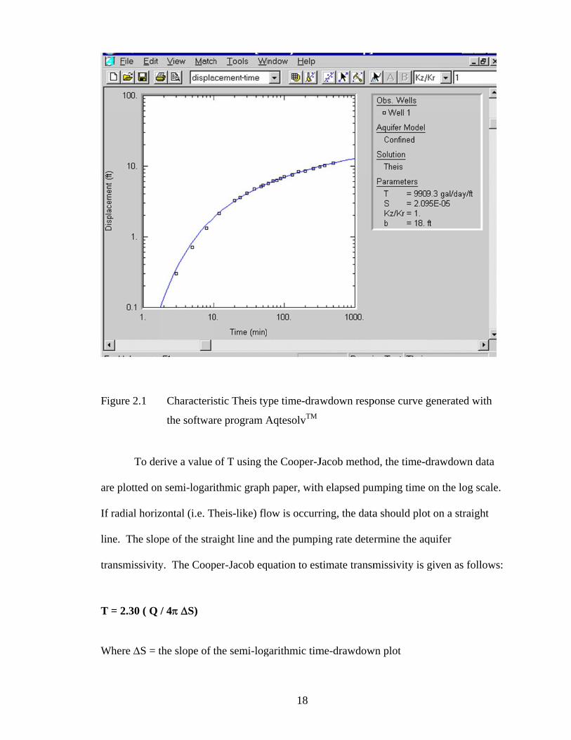
igure 2.1
To der
re plotted on
f radial horiz
ne. The slop
ransmissivity
T = 2.30 ( Q
Where S = t
Characteri
the softwar
rive a value
n semi-logari
zontal (i.e. T
pe of the stra
y. The Coop
/ 4 S)
the slope of t
stic Theis ty
re program A
of T using t
ithmic graph
Theis-like) flo
aight line an
per-Jacob eq
the semi-log
18
ype time-draw
AqtesolvTM
he Cooper-J
h paper, with
ow is occurr
nd the pumpi
quation to est
garithmic tim
wdown resp
Jacob metho
h elapsed pu
ring, the data
ing rate deter
timate transm
me-drawdow
ponse curve g
d, the time-d
umping time
a should plo
rmine the aq
missivity is g
wn plot
generated wi
drawdown d
on the log sc
t on a straigh
quifer
given as foll
ith
data
cale.
ht
lows:
19
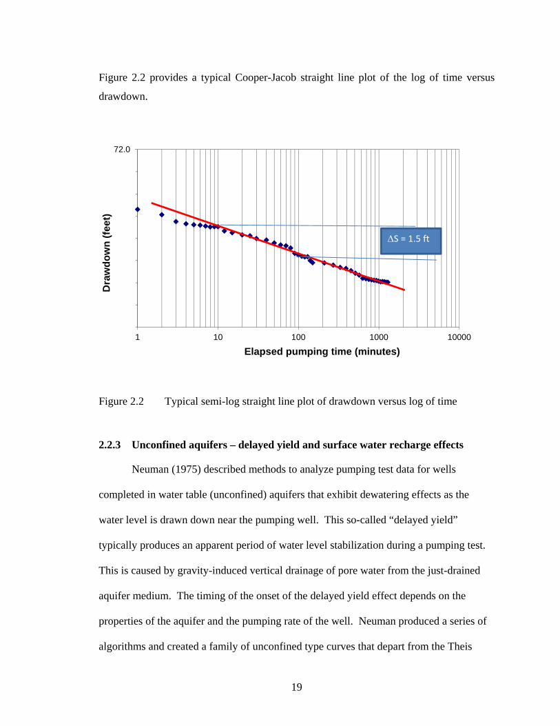
Figure 2.2 provides a typical Cooper-Jacob straight line plot of the log of time versus
drawdown.
Figure 2.2 Typical semi-log straight line plot of drawdown versus log of time
2.2.3 Unconfined aquifers – delayed yield and surface water recharge effects
Neuman (1975) described methods to analyze pumping test data for wells
completed in water table (unconfined) aquifers that exhibit dewatering effects as the
water level is drawn down near the pumping well. This so-called “delayed yield”
typically produces an apparent period of water level stabilization during a pumping test.
This is caused by gravity-induced vertical drainage of pore water from the just-drained
aquifer medium. The timing of the onset of the delayed yield effect depends on the
properties of the aquifer and the pumping rate of the well. Neuman produced a series of
algorithms and created a family of unconfined type curves that depart from the Theis
72.0
1 10 100 1000 10000
Dra
wd
ow
n (
feet
)
Elapsed pumping time (minutes)
S = 1.5 ft

20
curve in the middle part of the pumping test, but converge with the Theis curve late in the
test (assuming the test is run long enough). This convergence with ideal confined-like
behavior occurs when the bulk of the pore water drainage has been exhausted and the
cone of depression continues to slowly expand under radial flow conditions.
One of the shortcomings of the Neuman method, and modifications of the
Neuman method, summarized in Kruseman and de Ridder (1990) is that it does not
account for the additional drawdown that occurs near the pumping well and the
consequent reduction in near-well aquifer transmissivity due to dewatering. However,
the Neuman method is useful for observation wells located a distance from the tested well
that is at least greater than one unit of pre-pumping aquifer thickness (Allen 1999).
Neuman’s method is less useful in predicting the drawdown behavior in the pumping
well, which may be why some guidelines, including for example the CPCN Guidelines in
British Columbia and texts such as Driscoll (1986), recommend a minimum 72 hour
pumping test on wells in unconfined aquifers. After 2 or 3 days of pumping, the delayed
yield effect has usually run its course, and radial flow conditions exist enabling
conventional aquifer test analysis using, for example, the Cooper-Jacob method. The
aquifer coefficient of storage (specific yield in unconfined systems) is notoriously
difficult to estimate accurately with pumping test data, even when observation wells are
used in unconfined systems, with software programs giving unrealistic values, that may
be either too high (i.e. greater than 1) or too low (i.e. 1E-04). Many analysts simply
assume a value on the order of 1E-01 based on a typical effective porosity value.
Sometimes delayed yield is difficult to differentiate from leaky aquifer response
(Weight and Sonderegger 2001), and so an understanding of local geology and hydrology
is required to make such interpretation possible. In addition, it is common for unconfined
21
aquifers to be found and developed in close proximity to surface water sources. The
author’s experience in conducting pumping tests in shallow unconfined aquifers located
in such settings has found that the delayed yield effect may be difficult to differentiate
from surface water recharge boundary effects, because both delayed yield and induced
surface water recharge effects may produce a period of apparent water level stabilization,
and then as pumping continues, the cone of depression expands beyond the location of
the surface water recharge source, and the aquifer continues to behave as an ideal,
confined aquifer experiencing radial flow (i.e. a flat pressure derivative and a straight line
on a semi-log plot). This phenomenon has been observed to occur in situations where a
creek partially penetrates an unconfined aquifer and observation wells on the far side of
the creek from the pumping well experience drawdown during a pumping test. When the
source of surface water recharge is strong, then the well water level during a pumping test
may be observed to stabilize quickly (sometimes within a minute or two), and then does
not change unless the surface water level changes (Figure 2.3).
2.2.4 Linear and fracture flow models
Allen (1999) and Kruseman and de Ridder (1990) provide summaries of fracture
flow and linear flow analytical models. The response of observation wells to pumping
tests conducted in fractured bedrock aquifers with steeply-dipping (vertical) fractures is
also explored in an earlier paper by Gingarten and Witherspoon (1972). The linear flow
period is characterized as a straight-line on a log-log plot of time versus drawdown; and
has a 0.5 slope (Allen 1999). If pumping continues long enough and if the vertical
fracture behaves as a confined aquifer (i.e. is not significantly dewatered), then usually
the later time drawdown data may be analyzed by the Cooper – Jacob (1946) method.
According to Allen (1999), pumping tests in fractured bedrock wells exhibiting linear
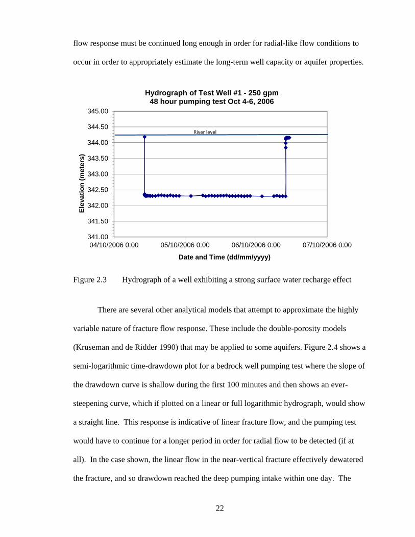
22
flow response must be continued long enough in order for radial-like flow conditions to
occur in order to appropriately estimate the long-term well capacity or aquifer properties.
Figure 2.3 Hydrograph of a well exhibiting a strong surface water recharge effect
There are several other analytical models that attempt to approximate the highly
variable nature of fracture flow response. These include the double-porosity models
(Kruseman and de Ridder 1990) that may be applied to some aquifers. Figure 2.4 shows a
semi-logarithmic time-drawdown plot for a bedrock well pumping test where the slope of
the drawdown curve is shallow during the first 100 minutes and then shows an ever-
steepening curve, which if plotted on a linear or full logarithmic hydrograph, would show
a straight line. This response is indicative of linear fracture flow, and the pumping test
would have to continue for a longer period in order for radial flow to be detected (if at
all). In the case shown, the linear flow in the near-vertical fracture effectively dewatered
the fracture, and so drawdown reached the deep pumping intake within one day. The
341.00
341.50
342.00
342.50
343.00
343.50
344.00
344.50
345.00
04/10/2006 0:00 05/10/2006 0:00 06/10/2006 0:00 07/10/2006 0:00
Ele
vati
on
(m
eter
s)
Date and Time (dd/mm/yyyy)
Hydrograph of Test Well #1 - 250 gpm 48 hour pumping test Oct 4-6, 2006
River level
ne
fl
F
2
w
fo
to
ex
su
pu
ext section d
low conditio
igure 2.4
.2.5 Pressu
The u
where analyst
ormation pre
o groundwat
xpanded upo
ummaries by
Pressu
umping test
discusses how
ns during a p
Hydrograp
test
ure derivati
se of pressur
ts devised di
essure respon
er resource s
on by Spane
y Allen (199
ure derivativ
analyst in ch
w pressure d
pumping tes
ph illustrating
ive analysis
re derivative
iagnostic too
nse to oilfiel
studies was n
and Wurstn
99) and Nevi
ve analysis is
hoosing whi
23
derivative an
st.
g probable l
e techniques
ols intended
ld operations
noted in earl
ner (1993), an
lle (2008).
s best describ
ich portion o
nalysis may b
inear flow in
evolved in t
to evaluate r
s. The appli
ly papers by
nd further di
bed as a diag
of a drawdow
be used to id
n a bedrock
the petroleum
reservoir ge
ication of de
y Bourdet et
iscussed in s
gnostic tool
wn or recove
dentify radia
well pumpin
m industry,
ometry and
rivative anal
al. (1989);
subsequent
to assist the
ery curve to u
al
ng
lysis
use
24
to derive aquifer hydraulic properties. As noted by Allen (1999), an infinitely acting
radial flow regime (i.e. Theis-like flow) has no characteristic behavior on a type curve,
but the logarithm of the derivative of drawdown (head) takes on a particular recognizable
shape when plotted on a log-log plot against the log of elapsed pumping time. In essence,
a pressure derivative plot is a log-log plot of a semi-logarithmic plot of time versus
drawdown (Figure 2.2 is a semi-log plot). Derivative plots make it relatively easy to
differentiate portions of a pumping test where linear or vertical flow may be occurring,
and when key assumptions in a Theis or Cooper-Jacob analysis are not met due to casing
storage, boundary effects, or other non-ideal conditions.
Typical characteristic features of derivative plots include a rising linear slope in
early time (usually the first few minutes of a pumping test) indicating casing storage
effects, a flat or mostly flat derivative indicative of radial (Theis-like) flow, a falling
derivative indicative of a leaky aquifer or recharge boundary effect, or a rising derivative
indicating a linear no flow boundary. Coupled with the conceptual model of the well site
hydrogeology, other effects such as non-Darcy conditions caused by vertical flow (such
as in a bedrock fracture or in an unconfined aquifer with large drawdowns) may be
identified.
Figure 2.5 (Page 26) provides an example pressure derivative plot as generated by
a spreadsheet tool developed and included in the Allen (1999) paper. This “DERIV”
spreadsheet includes a fixed end-point algorithm that calculates the pressure derivative
from basic elapsed time and drawdown data collected during a pumping test. This
algorithm is less complex than the least-squares regression algorithm included with
software programs (such as AqtesolvTM), but when the quality of data is good, the
spreadsheet provides an effective diagnostic curve. The worksheet also displays semi-
25
logarithmic and logarithmic time-drawdown plots. The DERIV fixed end-point
algorithm calculates the first-order derivative of head (drawdown), with respect to the
natural log of the change in time, using 3 data points (the point of interest and the ones
immediately preceding and following that point). The mathematical expression used to
calculate the pressure derivative is from Spane and Wurstner (1993) and is as follows:
(dp / dX)1 = [ (P1 / X1)X2 + (P2 / X2) X1] / (X1 + X2)
The 1 and 2 subscripts refer to the data points before and after the point of interest, P is
pressure and X is time. Three columns of data are normally input into the DERIV sheet:
time, water level and drawdown. Figure 2.6 shows a composite plot of a log-log (Theis)
plot of time and drawdown and the corresponding pressure derivative, as generated by the
commercial software package AqtesolvTM.
One additional point on derivative plots is that a late-time “end effect” is common
(Spane and Wurstner 1993) and is characterized by increased noise in the data caused by
a combination of factors including the relatively small rate of drawdown occurring in
later time, and the amount of remaining drawdown data at the point of calculation. If
necessary, this may sometimes be addressed by varying the L-spacing if the fixed end-
point algorithm is used. Software programs providing derivative curves have automated
smoothing routines to help deal with end-effect data scatter .
F
igure 2.5 Pressure dderivative ch
26
aracteristics (modified aafter Allen 1999)
F
2
va
w
pu
m
igure 2.6
.2.6 Step p
Before
ariable-rate
water supply
umping rate
measuring we
Composite
crosses)
pumping tes
e moving on
or step pump
wells and in
s that are he
ell drawdow
e plot of The
sts
n to discuss w
ping tests is
nvolve opera
ld constant f
wn (Weight an
27
eis curve (blu
well yield de
in order. Su
ating the test
for anywhere
nd Sondereg
ue boxes) an
etermination
uch tests are
pump at thr
e from 30 m
gger 2001).
nd pressure d
n methods, a
e commonly
ree or more d
minutes to 2 h
The relative
derivative (re
brief review
performed o
different
hours while
e specific
ed
w of
on
28
capacity (flow rate divided by drawdown) of the well at the end of each pumping step is
then determined. Besides giving a general indication of the well’s performance, the step
test provides potentially critical information having implications on the long term
capacity of the well.
The concept of well efficiency is sometimes used to assess the results of step tests
(Driscoll 1986). What this actually means is the proportion of drawdown in the well
caused by laminar (Darcian) flow relative to the proportion of drawdown caused by non-
laminar (turbulent) flow. When most of the drawdown (or well loss) is caused by laminar
flow, then the drawdown in the well varies in proportion to flow rate and the well is
considered hydraulically efficient. Significant drawdown caused by turbulent flow means
that some of the drawdown varies in proportion to some exponent of the flow rate. The
basic equation, developed by Jacob (1946) and given by Driscoll (1986) is as follows:
s (drawdown) = BQ + CQ2 where
B = the laminar well loss coefficient
C = the turbulent well loss coefficient
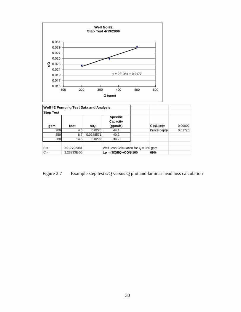
When step test data are plotted on a linear graph with the ratio of drawdown to flow rate
(s/Q, which is the inverse of specific capacity) plotted on the y axis and the flow rate (Q)
on the horizontal axis, the slope of the line is C and the y intercept is B. The exponent
applied to the CQ term is for convenience taken to be 2 (Driscoll 1986) but actually
varies depending on the hydraulics of the well. The BQ term can be inferred as the
drawdown occurring due to laminar flow in the aquifer near the well and the CQ2 term is
inferred to be the head loss due to turbulent flow as groundwater enters the well through
the well screen openings or in bedrock wells, fracture openings. One expression of the
29
empirical “well efficiency” is derived with the following equation (Driscoll 1986;
Kruseman and de Ridder 1990):
Lp = (BQ/BQ+CQ2) x 100 (expressed as a percentage)
The Lp term is the percentage of well drawdown due to laminar flow loss and Figure 2.7
provides a s/Q versus Q plot and a sample calculation. For a reasonably efficient well
that is not being over-pumped, the data should plot on a straight line as shown. If the
higher flow rate s/Q values do not plot on the straight line, then this could indicate
increased turbulent head loss (non-laminar flow) at higher pumping rates.
As shown later, some of the empirical equations for determining safe well yield
(LTWC) may produce a theoretical value that far exceeds the test pumping rate. Because
it is possible that a non-linear relationship between pumping rate and drawdown could
exist at higher pumping rates, it is generally not a good idea to extrapolate a calculated
well capacity beyond the rate at which a pumping test or step test has confirmed a
laminar flow condition.
F
BC
W
S
igure 2.7
gpm200350500
B = 0.0C = 2.2
Well #2 Pumpin
Step Test
Example s
feet s4.58.7 0.0
14.6
01770238123333E-05
ng Test Data a
step test s/Q
s/Q
SpCa(g
0.02250248571
0.0292
Well Lo
Lp = (B
and Analysis
30
versus Q plo
pecific apacity pm/ft)44.440.234.2
oss Calculation fo
BQ/BQ +CQ2)*10
ot and lamin
C (sloB(inte
or Q = 350 gpm
00 69%
nar head loss
ope)= 0.ercept)= 0.
s calculation
0000201770
31
CHAPTER 3
PREVIOUS WORK ON WELL YIELD DETERMINATION METHODS
As noted in the introduction concepts of Safe Aquifer Yield and Sustainable
Groundwater Yield have been widely described, analyzed and debated in the literature,
while by comparison, the Long Term Well Capacity (i.e. the safe yield of individual
wells) has received relatively little attention. This is probably due to the fact that SAY
and SGY involve theoretical approaches, whereas LTWC requires application of
empirical methodologies, although these may be based on basic groundwater theory, such
as radial flow to a well (e.g., Theis, 1935).
A search of literature sources including those available via internet search engines
such as Google, as well as the publication search functions of the National Ground Water
Association (NGWA); and International Association of Hydrogeologists (IAH); and
numerous U.S. State and Canadian Provincial data bases and government websites
revealed that there are a number of published methodologies or guidelines that are used to
determine the long-term “safe” capacity or yield of a well. Some of these are categorized
here as “quantitative” in that they use traditional analytical pumping test analysis (for
example, determination of the slope of a drawdown curve on a semi-logarithmic plot) and
use some type of numerical equation to determine well capacity as a function of pumping
time and available drawdown in the well.
Other methods include those that consist of variations on volume-based
determinations, which are relatively simplistic, and provide a means to estimate well
capacity with little or no hydrogeologic expertise needed. Some guidelines appear to
leave the question of determining the well yield to the judgement of a well driller or a
hydrogeologist, without providing any suggested or required methodology. Examples of
32
the various types of well capacity determination methodologies known to be in use in
North America follow in the next two subsections. It is not known why numerous
government jurisdictions having some form of regulatory control over groundwater use
seem to have avoided the adoption of a standard methodology to estimate well capacity,
or why most of the methods that do exist are from western Canada (Maathuis and van der
Kamp 2006). This is true even for jurisdictions such as Ontario (2005a; 2005b) that have
published fairly detailed (and sometimes prescriptive) well pumping test procedures, but
have no quantitative methodology to determine long-term well capacity using pumping
test data.
3.1 QUANTITATIVE METHODS BASED ON RADIAL FLOW THEORY
Several quantitative (equation-based) methods exist for the estimation of long-
term well capacity or “safe well yield.” Although empirical, these methods are founded in
the fundamental scientific principles of radial flow to pumping wells, as originally
described by Theis (1935). This section describes the three methods evaluated in detail in
this study which are herein described as Methods A, B and C. Other empirical,
volumetric or professional judgement-based methods are described in Chapter 3.2.
3.1.1 Theoretical background to the quantitative methods
There are several quantitative well yield estimation methods that are based on
fundamental well and aquifer hydraulic principles, such as the Theis formula. The
methods determine LTWC primarily as a function of the aquifer transmissivity and the
pumping duration. Implicit in the use of these methods is the assumption (which should
be confirmed with step tests) that drawdown in well varies linearly with the flow rate, and
that the proportion of drawdown due to turbulent flow is relatively small.
33
The most widely used of the quantitative methods known in North America were
all developed in western Canada. These include methods first used in the prairie
provinces of Alberta and Saskatchewan (Farvolden and Moell); and more recent methods
developed in British Columbia (B.C. Ministry of Environment). van der Kamp and
Maathuis (2005) provided a review of the background on the first two methods, and also
recommended adoption of a new method to replace the older methods, which in a
subsequent publication (Maathuis and van der Kamp 2006) they termed the modified
Moell method.
As described in detail by van der Kamp and Maathuis (2005) the so-called Q20
methods (Q20 standing for the safe or sustainable 20 year well yield) is for the case when
the water level continues to decline during a pumping test, which indicates that the well is
drawing water from storage. Presumably, 20 years is selected as the time horizon
because this is sufficiently far in the future to allow for more study of the aquifer system
and more planning for water supply infrastructure; it may also be tied to the groundwater
licensing procedure in Alberta, where most groundwater use permits are typically up for
renewal after 20 years. The rationale of the Q20 methods, then, is that if the well needs to
last at least 20 years (which is about 10 million minutes), the drawdown curve when
projected should not exceed the total available drawdown in the well (less a safety
factor). In addition to the practical consideration of needing to allow for some minimum
submergence of the well pump below the pumping water level, the use of a safety factor
accounts for natural variability in groundwater and well systems, and also is a way to
address uncertainty in the data analysis. Practitioners have somewhat arbitrarily selected
a 70% (0.7) safety factor for use in calculating LTWC values.

34
When applied in the context of actual hydrogeologic conditions and groundwater
use, the Q20 method could be conservative, because wells are generally not pumped
continuously, and storage depletion is not the only source of water since aquifers may
receive some amount of natural or induced recharge at some point each year. However,
in cases where aquifer depletion is possible, such as highly confined aquifers, aquifers in
dry climates, or situations of known groundwater decline (e.g. the High Plains Aquifer
system in the U.S.), then the Q20 method might provide either a realistic or even an
optimistic estimation of long-term well yield. Any method of determining LTWC could
lead to overestimates when the combined effects of multiple well withdrawals lead to
yearly declines in groundwater levels. In such cases, a Q20 determination would need to
be adjusted (downward) to account for cumulative and progressive aquifer depletion.
Relating well capacity to loss of available drawdown (or saturated thickness) has been
explored in Kansas (Hecox et al. 2002) for the specific case of the Ogallala aquifer
portion of the High Plains aquifer system.
The fundamental assumption in making long-term projections of well drawdown
from pumping test data is that the drawdown trend is predictable, and importantly,
conforms to the line predicted by the Theis (1935) and/or Cooper-Jacob (1946) methods
for non-equilibrium pumping tests. This is conveniently taken to be in the form of a
straight line when the time-versus-drawdown data are plotted on semi-logarithmic graph
paper as shown in the example in Figure 3.1. van der Kamp and Maathuis (2005; 2006)
noted that the idealized aquifer model of homogeneity and infinite extent is not always
met, which might cause predictive uncertainty.
For a Q20 determination, there are eight log cycles of time between 1/10th of a
minute and 10 million minutes. So for a total available drawdown of HA, 1/8th of that

am
ap
m
3
19
an
da
ob
C
F
mount is ava
pproximatio
may then be d
.2 illustrates
For a
999; see 3.1
n aquifer bou
ays, and then
btaining a pe
Convenience
igure 3.1
ailable durin
n is valid for
determined a
s some of the
100-day yie
.4) projects t
undary cond
n applies a 0
ermit to oper
and Necessi
Semi-logar
linear (y ax
ng each log c
r the entire 2
as described
e terms used
ld determina
the latest con
dition) to 100
0.7 safety fac
rate a water
ity (CPCN) i
rithmic plot
xis) scale
35
cycle of time
20 year perio
by the equa
in the LTW
ation, the Br
nfirmed draw
0 days, calcu
ctor. This ap
utility, whic
in B.C.
of time on l
e. Assuming
od, the “safe
ations in the
WC methods.
ritish Columb
wdown trend
ulates the we
pproach is b
ch is called a
og scale and
g the Cooper
e pumping ra
following se
bia method (
d (even if it
ell specific c
ased on guid
a Certificate
d water level
r-Jacob
ate” of the w
ections. Figu
(Allen et al.
is a trend du
capacity at 10
delines for
of Public
l or drawdow
well
ure
ue to
00
wn on

36
The CPCN method does not explicitly require the hydrogeologist to assume that
Theis-like conditions (i.e. radial flow) persist for 100 days of pumping, since by
definition a boundary condition is indicative of either a no-flow boundary, a recharge
boundary, or a significant change in aquifer properties at some distance from the
pumping well such that the key assumptions of the Theis and Cooper-Jacob methods are
not being met (e.g., horizontal aquifer, homogenous properties, infinite in areal extent,
and so on). However, the CPCN method does require that the later time data fall on a
straight line and so the method cannot be applied if multiple boundary effects are noted in
the test data, or if the data plot on a straight line on an arithmetic hydrograph or exhibit an
ever-steepening trend on a semi-logarithmic time-drawdown plot (see Figure 2.4). Like
the Q20 methods, the CPCN method is conservative in that it assumes no recharge and
that the well is drawing water from storage (in cases where the data plot on a straight line
with no boundary conditions).

37
Figure 3.2 Semi-logarithmic plots showing S and HA values, and a straight-line
drawdown projection
60.0
70.0
80.0
90.01 10 100 1000 10000 100000
Dep
th t
o W
ater
(fe
et)
Elapsed time (minutes)
1 daystatic water level = 64.5 ft
HA = 25.5 ft
60.0
70.0
80.0
90.01 10 100 1000 10000 100000
Dep
th t
o W
ater
(fe
et)
Elapsed time (minutes)
1 daystatic water level = 64.5 ft
HA = 25.5 ft
S = 1.8 ft
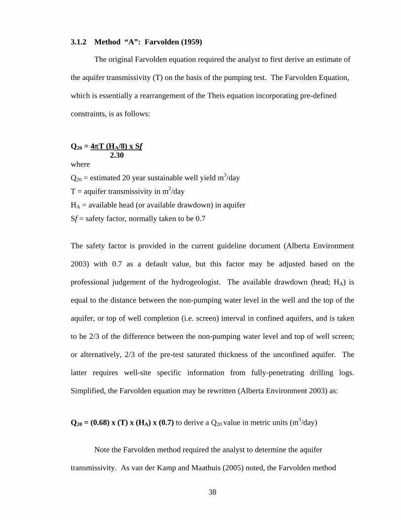
38
3.1.2 Method “A”: Farvolden (1959)
The original Farvolden equation required the analyst to first derive an estimate of
the aquifer transmissivity (T) on the basis of the pumping test. The Farvolden Equation,
which is essentially a rearrangement of the Theis equation incorporating pre-defined
constraints, is as follows:
Q20 = 4T (HA/8) x Sf 2.30 where
Q20 = estimated 20 year sustainable well yield m3/day
T = aquifer transmissivity in m2/day
HA = available head (or available drawdown) in aquifer
Sf = safety factor, normally taken to be 0.7
The safety factor is provided in the current guideline document (Alberta Environment
2003) with 0.7 as a default value, but this factor may be adjusted based on the
professional judgement of the hydrogeologist. The available drawdown (head; HA) is
equal to the distance between the non-pumping water level in the well and the top of the
aquifer, or top of well completion (i.e. screen) interval in confined aquifers, and is taken
to be 2/3 of the difference between the non-pumping water level and top of well screen;
or alternatively, 2/3 of the pre-test saturated thickness of the unconfined aquifer. The
latter requires well-site specific information from fully-penetrating drilling logs.
Simplified, the Farvolden equation may be rewritten (Alberta Environment 2003) as:
Q20 = (0.68) x (T) x (HA) x (0.7) to derive a Q20 value in metric units (m3/day)
Note the Farvolden method required the analyst to determine the aquifer
transmissivity. As van der Kamp and Maathuis (2005) noted, the Farvolden method

39
assumes radial flow conditions, which means the long-term drawdown would follow the
trend predicted by the Theis (1935) equation or the Cooper-Jacob (1946) approximation
to the Theis equation for a confined aquifer. If this is the case, then the Farvolden
equation may be rewritten as suggested by van der Kamp and Maathuis (2005) as:
Q20 = 0.7 x HA x Qt/8Sp
where:
Qt = test pumping rate
8Sp = eight log cycles of drawdown (i.e. 0.1 to 10E+06 minutes, which equals 6,944
days or about 19 years and 9 days, which for convenience is apparently rounded to 20
years).
HA and Sf as defined above
A key assumption of the Farvolden method is that the earliest drawdown, in
particular the drawdown in the first 6 seconds and even the first minute (i.e. the first log
cycle of time in most tests) is infinitesimally small compared to the total drawdown
during the pumping test. When this is not the case, the Farvolden method might lead to
an underestimation of the projected 20 year drawdown, and consequently, an overly-
optimistic well capacity estimate. The effect of under-predicting the initial log cycle of
drawdown is to displace the drawdown curve vertically upward such that all of the future
drawdown values are underestimated. Published information on the Farvolden method
does not provide a way to check the validity of the results when applied to a specific well
test.

40
3.1.3 Method “B”: Moell (1975)
Recognizing that in some cases, large drawdowns may occur early in the pumping
test, Moell (1975) derived an alternative formula that projects the drawdown trend as
observed 100 minutes into the test out to 20 years. The Moell equation provided in
Alberta Environment (2003) is as follows:
Q20 = Sf (0.7) x HA x Qt / (S100min + 5S)
This method does not require the analyst to derive an aquifer transmissivity value to
estimate the theoretical long-term well yield (though elsewhere in Alberta Environment
2003, this is required for hydrogeological reports).
3.1.4 Method “C”: B.C. Ministry of Environment (1999)
Whereas the Q20 methods were developed in part to standardize safe well yield
calculations for the purposes of groundwater licensing (water right permitting), British
Columbia has to date not required a water right permit or license to extract groundwater.
However, there is some regulation of groundwater use extraction through water utility
legislation. This legislation and associated regulations and guidelines require private
water utilities to license their water system by obtaining a CPCN permit.
Following enactment of the water utility regulation, the B.C. government in the
1990s developed guidelines for the regulated water utilities to follow. These guidelines
included standards for groundwater well assessments, including design, analysis and
reporting of aquifer pumping tests. Allen et al. (1999) prepared a report for the B.C.
Ministry of Environment that became the basis for the CPCN groundwater evaluation
guidelines. These guidelines include a specified method for determining a 100-day well
capacity, termed the long term well capacity, for wells proposed to serve water utilities.

41
The scientific basis of the equation used is similar to the Q20 methods in that it
requires a determination of the slope of the time-drawdown curve on a semi-logarithmic
plot and directs the analyst to project the late-time drawdown trend to 100 days, from
which the theoretical 100-day specific capacity is calculated. The CPCN method applies a
70 percent (i.e. 0.70) safety factor, and also requires minimum 24-hour pumping tests,
and calls for 72-hour pumping tests in unconfined aquifers and in fractured bedrock
formations. The CPCN well capacity formula for a 100-day LTWC (Q100d) is provided
below:
Q100d = Sf (0.7) x HA x (Qt/S100)
The available drawdown term, which for consistency with the previous Q20
methods is abbreviated here by the term HA, is defined in the CPCN guidelines. For
fractured bedrock formations, this is taken to be the difference between the non-pumping
(static) water level and the uppermost water-bearing fracture if one is noted on the well
driller’s log. In lower-yielding bedrock wells, where fractures are difficult to detect
during drilling, normally a depth of 10 to 20 feet from the bottom of the hole is taken to
be the fracture depth, based on the presumption that with low-yielding wells, the driller
stopped soon after encountering a water-bearing fracture.
In other types of confined and unconfined aquifers, for example alluvial or glacial
sedimentary systems, the available drawdown is the difference between the static water
level and the top of the confined aquifer, or the top of the well screen, whichever is
shallower. The 70% safety factor (0.7) is intended to allow for seasonal variations in
water levels, well interference (unless this causes major additional drawdown), adequate
submergence for the well pump, and possible declines in well performance.
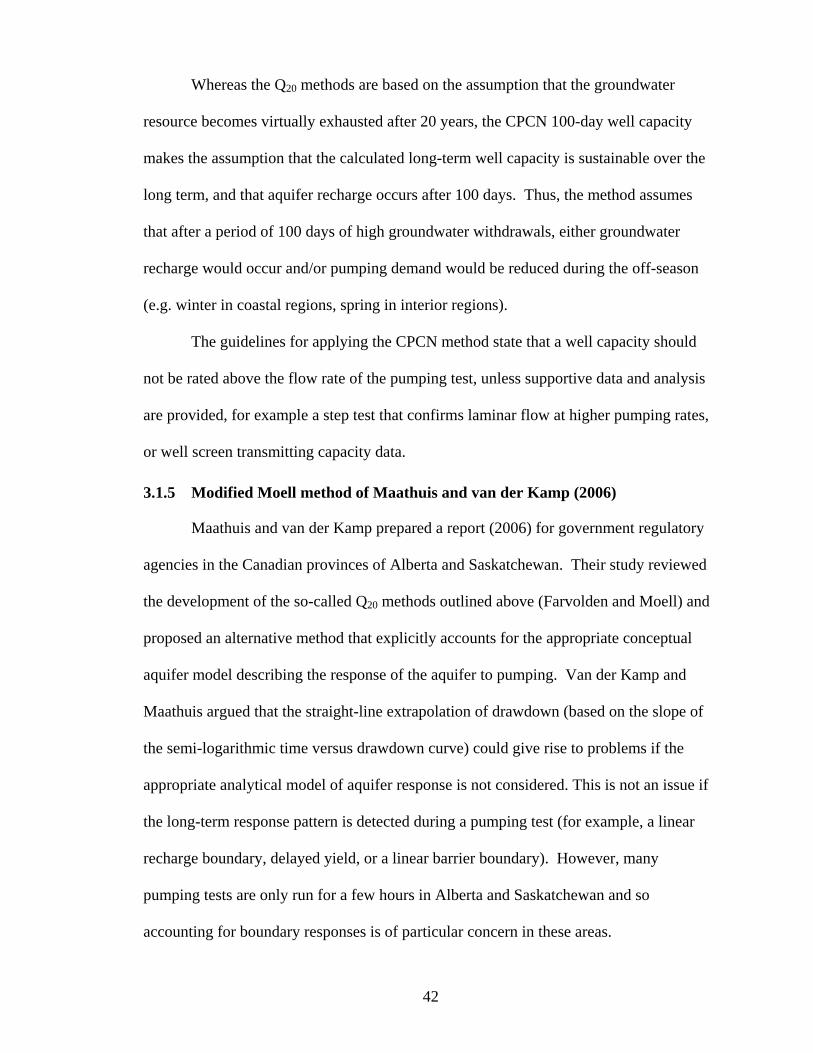
42
Whereas the Q20 methods are based on the assumption that the groundwater
resource becomes virtually exhausted after 20 years, the CPCN 100-day well capacity
makes the assumption that the calculated long-term well capacity is sustainable over the
long term, and that aquifer recharge occurs after 100 days. Thus, the method assumes
that after a period of 100 days of high groundwater withdrawals, either groundwater
recharge would occur and/or pumping demand would be reduced during the off-season
(e.g. winter in coastal regions, spring in interior regions).
The guidelines for applying the CPCN method state that a well capacity should
not be rated above the flow rate of the pumping test, unless supportive data and analysis
are provided, for example a step test that confirms laminar flow at higher pumping rates,
or well screen transmitting capacity data.
3.1.5 Modified Moell method of Maathuis and van der Kamp (2006)
Maathuis and van der Kamp prepared a report (2006) for government regulatory
agencies in the Canadian provinces of Alberta and Saskatchewan. Their study reviewed
the development of the so-called Q20 methods outlined above (Farvolden and Moell) and
proposed an alternative method that explicitly accounts for the appropriate conceptual
aquifer model describing the response of the aquifer to pumping. Van der Kamp and
Maathuis argued that the straight-line extrapolation of drawdown (based on the slope of
the semi-logarithmic time versus drawdown curve) could give rise to problems if the
appropriate analytical model of aquifer response is not considered. This is not an issue if
the long-term response pattern is detected during a pumping test (for example, a linear
recharge boundary, delayed yield, or a linear barrier boundary). However, many
pumping tests are only run for a few hours in Alberta and Saskatchewan and so
accounting for boundary responses is of particular concern in these areas.
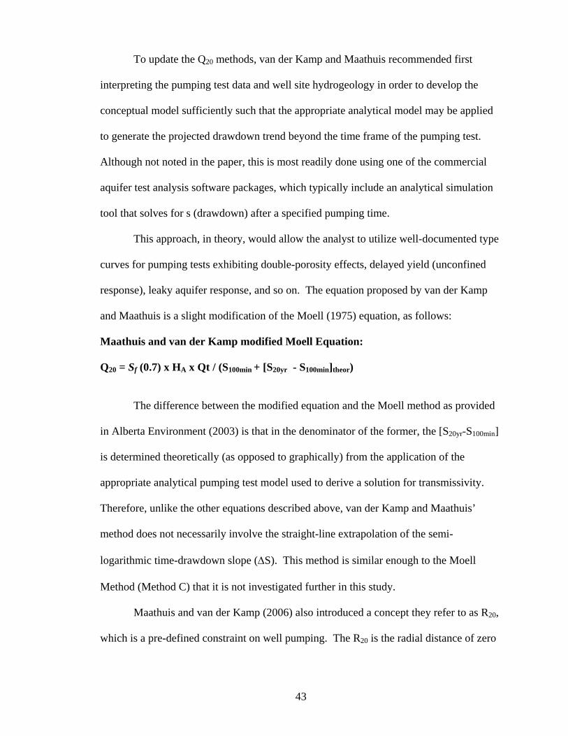
43
To update the Q20 methods, van der Kamp and Maathuis recommended first
interpreting the pumping test data and well site hydrogeology in order to develop the
conceptual model sufficiently such that the appropriate analytical model may be applied
to generate the projected drawdown trend beyond the time frame of the pumping test.
Although not noted in the paper, this is most readily done using one of the commercial
aquifer test analysis software packages, which typically include an analytical simulation
tool that solves for s (drawdown) after a specified pumping time.
This approach, in theory, would allow the analyst to utilize well-documented type
curves for pumping tests exhibiting double-porosity effects, delayed yield (unconfined
response), leaky aquifer response, and so on. The equation proposed by van der Kamp
and Maathuis is a slight modification of the Moell (1975) equation, as follows:
Maathuis and van der Kamp modified Moell Equation:
Q20 = Sf (0.7) x HA x Qt / (S100min + [S20yr - S100min]theor)
The difference between the modified equation and the Moell method as provided
in Alberta Environment (2003) is that in the denominator of the former, the [S20yr-S100min]
is determined theoretically (as opposed to graphically) from the application of the
appropriate analytical pumping test model used to derive a solution for transmissivity.
Therefore, unlike the other equations described above, van der Kamp and Maathuis’
method does not necessarily involve the straight-line extrapolation of the semi-
logarithmic time-drawdown slope (S). This method is similar enough to the Moell
Method (Method C) that it is not investigated further in this study.
Maathuis and van der Kamp (2006) also introduced a concept they refer to as R20,
which is a pre-defined constraint on well pumping. The R20 is the radial distance of zero

44
drawdown (or some other defined value of drawdown) that may be used to constrain the
pumping rate or to identify a suitable radius from the tested well where other
groundwater uses should be considered in a groundwater management framework.
Application of the R20 concept may be used to make more conservative estimates of Q20
when, for example, it is desired to minimize drawdown at another well, or under a
sensitive stream. Maathuis and van der Kamp suggest that wells with R20 values
extending out considerable distances and encompassing many other wells or surface
water features could require further analysis beyond a simple well test Q20 calculation.
3.2 OTHER METHODS
In the absence of guidelines or regulations governing how a well’s long term
capacity is determined, in some jurisdictions hydrogeologists may use professional
judgement combined with analytical or numerical methods to assess well or aquifer
capacity. Some examples of these various techniques follow, included here for
completeness but not evaluated against Methods A, B and C.
3.2.1 Pumping test analytical simulation
This approach involves calculation of transmissivity and storativity from a
pumping test, and then using these derived constants to model well drawdown trend at
varying pumping rates, and extrapolating the drawdown trend out to a future point of time
of interest (e.g. 120 days for a full irrigation or peak demand season). This is
conceptually similar to the method advocated by Maathuis and van der Kamp (2006). If
the projected drawdown at a given pumping rate remains above the pump intake or the
top of the aquifer (with an appropriate safety factor applied), then the modeled pumping
rate is deemed sustainable. This technique also lends itself to relatively straightforward
application of the principle of superposition, from which the effects of multiple well
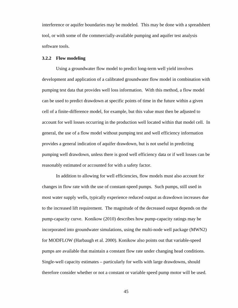
45
interference or aquifer boundaries may be modeled. This may be done with a spreadsheet
tool, or with some of the commercially-available pumping and aquifer test analysis
software tools.
3.2.2 Flow modeling
Using a groundwater flow model to predict long-term well yield involves
development and application of a calibrated groundwater flow model in combination with
pumping test data that provides well loss information. With this method, a flow model
can be used to predict drawdown at specific points of time in the future within a given
cell of a finite-difference model, for example, but this value must then be adjusted to
account for well losses occurring in the production well located within that model cell. In
general, the use of a flow model without pumping test and well efficiency information
provides a general indication of aquifer drawdown, but is not useful in predicting
pumping well drawdown, unless there is good well efficiency data or if well losses can be
reasonably estimated or accounted for with a safety factor.
In addition to allowing for well efficiencies, flow models must also account for
changes in flow rate with the use of constant-speed pumps. Such pumps, still used in
most water supply wells, typically experience reduced output as drawdown increases due
to the increased lift requirement. The magnitude of the decreased output depends on the
pump-capacity curve. Konikow (2010) describes how pump-capacity ratings may be
incorporated into groundwater simulations, using the multi-node well package (MWN2)
for MODFLOW (Harbaugh et al. 2000). Konikow also points out that variable-speed
pumps are available that maintain a constant flow rate under changing head conditions.
Single-well capacity estimates – particularly for wells with large drawdowns, should
therefore consider whether or not a constant or variable speed pump motor will be used.
46
The above approaches allow for considerable flexibility in the technique applied
by the analyst using professional judgement in the process of determining well yield.
This means that potentially, significantly different findings are possible based on
independent analysis of a given pumping test data set by two or more hydrogeologists.
Some government regulatory agencies, particularly in western Canada, in an effort to
achieve more consistency in the interpretation of well yield characteristics from pumping
tests have developed approaches that comprise the focus of the comparative analysis
portion of this research project.
3.2.3 Volumetric and other pumping test-based methods
Examples of other methods of determining well yield may be found in many
government regulatory and guidance documents. These may consist of non-prescriptive
directives, calling for a pumping test and a determination of well yield by a qualified
individual, such as a hydrogeologist (Ontario Ministry of Environment, 2005a, 2005b) or
a guidance document for private wells that provides only a cursory overview of well
testing (State of Connecticut 2009). Other jurisdictions provide a prescriptive volumetric
methodology for determining well yield.
For example, the Los Angeles County (California) Department of Public Health
(2005) guidelines for determining well yield stipulate a pumping test followed by a
recovery test, and state that the yield of the well is the recovery rate following pumping
cessation if less than full recovery occurs after a period of time equal to the pumping
duration. Thus, typically, a pro-rated portion of the pumping test withdrawal rate is taken
to be the long-term well yield. This method does not require the analyst to determine
whether or not radial flow conditions occurred, or whether or not aquifer boundary
conditions, well interference, or other effects are apparent in the pumping test data. For
47
these reasons, this type of volumetric method is probably too simplistic for broad
application, especially in complex settings where there are numerous wells, where there
is potential for well interference, large seasonal changes in water levels, and where longer
term pumping may induce changes in the system.
The volume test used in L.A. County requires a 24-hour pumping test, with the
flow rate and the total volume pumped recorded along with water levels before, during
and after the pumping test. The permitted long term yield of the well is the total gallons
pumped for 24 hours provided that full recovery occurs within 24 hours of pumping
cessation. If full recovery does not occur, the allowable yield is equal to the flow rate for
the 24 hour test, divided by the total number of minutes required to achieve full recovery.
If full recovery does not occur within five days, then the well is considered non-
sustainable. Full recovery is defined as 90 percent of the initial pre-test static water level.
Application of hydrogeological principles is not required. An example application of this
method for a well completed in a confined aquifer follows:
Hypothetical well volume test
A. Total well depth: 200 ft.
B. Depth to top of aquifer: 170 ft
C. Initial static water level: 15.0 ft
D. Test duration: 24 hours
E. Maximum water level: 94.6 ft. (at time t equal to 24 hrs)
F. Pumping rate (gpm) 100
G. Final recovery reading 16.1 ft (at time t’ equal to 48 hrs from start
of pumping test)
H. Maximum drawdown (E-C ): 79.6 ft
I. Amount of recovery: (G-B) 78.5 ft
J. Percent recovery (I / H) 99 %
K. Volume pumped = 144,000 gallons / day (100 gpm) = allowable yield
48
The Township of Langley, British Columbia has a bylaw (Township of Langley
2010) regulating private domestic wells and prescribes a four-hour pumping test method
to determine well yield. The well test must be performed at a minimum flow rate of 9
liters per minute (about 2.4 US gallons per minute) and uses the drawdown recorded after
10 minutes and 240 minutes of pumping to verify that the well can yield at least 1.74
liters per minute if pumped continuously for 30 days. The method plots the drawdown
data on a semi-logarithmic hydrograph of drawdown versus the log of elapsed pumping
time. A straight line projection is made by connecting the 10-minute and 240-minute
drawdown and extending this line to 30 days (43,200 minutes).
The static depth to water, plus the 30-day projected drawdown, plus an assumed
seasonal water level decline and a safety factor (usually 1 meter) must not exceed the
depth to the well pump intake. The local hydrogeology in the Langley area is such that
private domestic wells are completed in a stratified glacial-drift aquifer that is usually
productive relative to the requirements of a private household well. This method may be
useful locally, but is not considered to be adequate for higher capacity wells or wells that
would be pumped continuously for long periods, such as municipal, industrial or
irrigation wells.
A last example is found in the State of Vermont Water Supply Rules (2010),
which provide a definition of safe yield for pumped groundwater sources serving
community water systems. This flow rate can be no greater than the pumping test rate
and must be able to be met by public water supply well sources for a period of 180 days
at the projected water system average day demand, followed by a 3 or 7-day period of
pumping at the projected system maximum day demand. The Vermont rules, however,
do not provide a means to calculate the safe well yield other than the well source’s total
49
available drawdown must not be exceeded during the specified 183 or 187-day pumping
period. In practice, this is typically demonstrated using conventional pumping test
analysis. No safety factor or equation is provided for in the Vermont rules, but the rules
do provide detailed procedures for conducting both step rate and constant rate pumping
tests (72 to 120 hours in duration), and also detailed requirements for assessing potential
well interference.
3.2.4 Equilibrium (stabilized drawdown)
Occasionally, it is possible to determine the long-term well capacity if true
equilibrium conditions are encountered during a pumping test. This may occur if the
flow rate of the well is small relative to the transmissivity of the aquifer, or more
commonly, when the well is completed in an aquifer with a strong connection to a surface
water recharge source (Figure 2.3). The key technical issues to consider in making the
analysis of well capacity on the basis of equilibrium are: a) confirming that a stabilized
drawdown level continued long enough (i.e. more than a few hours), b) that the pumping
rate be held constant, and c) that the conceptual hydrogeological model supports the
stabilized well response. Farvolden (1959) provided a simple formula to estimate safe
well yield (Q20) for stabilized pumping tests:
Q20 = (Qt/s) * (HA) * ( Sf ) (Sf usually = 0.7), where s is the stabilized value of
drawdown.
The safety factor applied to the equilibrium well test data could be more
conservative (e.g. 0.5 or 0.6) if the HA value is small or if seasonal variation in water
level (groundwater or surface water) is unknown or believed to be significant relative to
available drawdown. The sensitivity of Q20 values to adjustments in the safety factor is
assessed in Chapter 5.
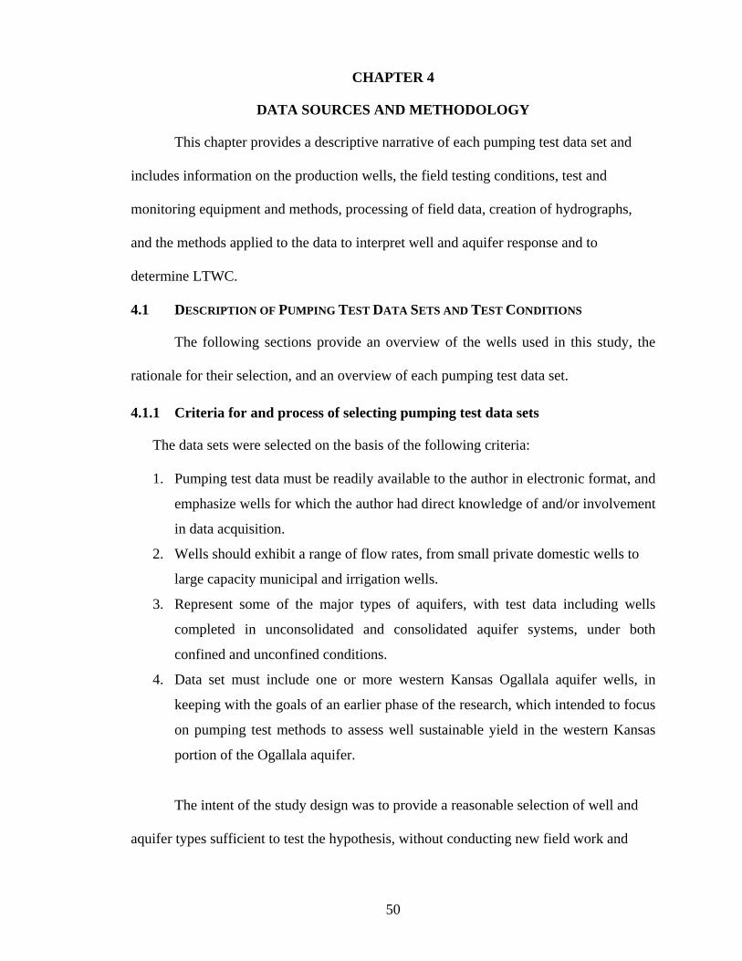
50
CHAPTER 4
DATA SOURCES AND METHODOLOGY
This chapter provides a descriptive narrative of each pumping test data set and
includes information on the production wells, the field testing conditions, test and
monitoring equipment and methods, processing of field data, creation of hydrographs,
and the methods applied to the data to interpret well and aquifer response and to
determine LTWC.
4.1 DESCRIPTION OF PUMPING TEST DATA SETS AND TEST CONDITIONS
The following sections provide an overview of the wells used in this study, the
rationale for their selection, and an overview of each pumping test data set.
4.1.1 Criteria for and process of selecting pumping test data sets
The data sets were selected on the basis of the following criteria:
1. Pumping test data must be readily available to the author in electronic format, and
emphasize wells for which the author had direct knowledge of and/or involvement
in data acquisition.
2. Wells should exhibit a range of flow rates, from small private domestic wells to
large capacity municipal and irrigation wells.
3. Represent some of the major types of aquifers, with test data including wells
completed in unconsolidated and consolidated aquifer systems, under both
confined and unconfined conditions.
4. Data set must include one or more western Kansas Ogallala aquifer wells, in
keeping with the goals of an earlier phase of the research, which intended to focus
on pumping test methods to assess well sustainable yield in the western Kansas
portion of the Ogallala aquifer.
The intent of the study design was to provide a reasonable selection of well and
aquifer types sufficient to test the hypothesis, without conducting new field work and
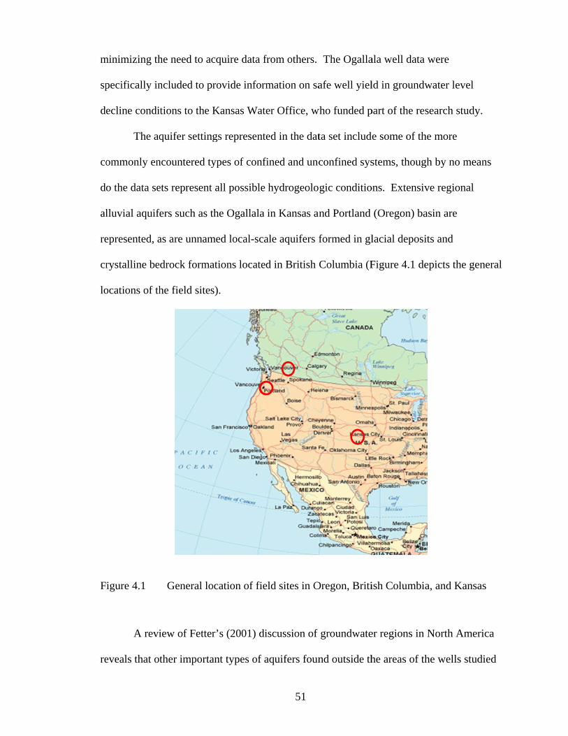
m
sp
de
co
do
al
re
cr
lo
F
re
minimizing th
pecifically in
ecline condi
The aq
ommonly en
o the data se
lluvial aquif
epresented, a
rystalline be
ocations of th
igure 4.1
A revi
eveals that o
he need to ac
ncluded to pr
itions to the K
quifer setting
ncountered ty
ets represent
fers such as t
as are unnam
edrock forma
he field sites
General lo
iew of Fetter
ther importa
cquire data f
rovide inform
Kansas Wat
gs represent
ypes of conf
all possible
the Ogallala
med local-sca
ations locate
s).
ocation of fie
r’s (2001) di
ant types of a
51
from others.
mation on sa
er Office, w
ed in the dat
fined and unc
hydrogeolo
in Kansas an
ale aquifers f
d in British
eld sites in O
iscussion of
aquifers foun
The Ogalla
afe well yiel
who funded p
ta set includ
confined sys
gic conditio
and Portland
formed in gl
Columbia (F
Oregon, Briti
groundwate
nd outside th
ala well data
ld in groundw
part of the re
e some of th
stems, thoug
ons. Extensiv
(Oregon) ba
lacial deposi
Figure 4.1 de
ish Columbi
er regions in
he areas of th
were
water level
search study
he more
gh by no mea
ve regional
asin are
its and
epicts the ge
a, and Kansa
North Amer
he wells stud
y.
ans
eneral
as
rica
died
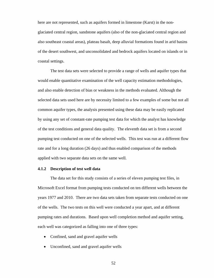
52
here are not represented, such as aquifers formed in limestone (Karst) in the non-
glaciated central region, sandstone aquifers (also of the non-glaciated central region and
also southeast coastal areas), plateau basalt, deep alluvial formations found in arid basins
of the desert southwest, and unconsolidated and bedrock aquifers located on islands or in
coastal settings.
The test data sets were selected to provide a range of wells and aquifer types that
would enable quantitative examination of the well capacity estimation methodologies,
and also enable detection of bias or weakness in the methods evaluated. Although the
selected data sets used here are by necessity limited to a few examples of some but not all
common aquifer types, the analysis presented using these data may be easily replicated
by using any set of constant-rate pumping test data for which the analyst has knowledge
of the test conditions and general data quality. The eleventh data set is from a second
pumping test conducted on one of the selected wells. This test was run at a different flow
rate and for a long duration (26 days) and thus enabled comparison of the methods
applied with two separate data sets on the same well.
4.1.2 Description of test well data
The data set for this study consists of a series of eleven pumping test files, in
Microsoft Excel format from pumping tests conducted on ten different wells between the
years 1977 and 2010. There are two data sets taken from separate tests conducted on one
of the wells. The two tests on this well were conducted a year apart, and at different
pumping rates and durations. Based upon well completion method and aquifer setting,
each well was categorized as falling into one of three types:
Confined, sand and gravel aquifer wells
Unconfined, sand and gravel aquifer wells

53
Fractured bedrock aquifer wells (may behave as confined)
The data set includes
a) Three relatively low-yielding wells completed in fractured crystalline bedrock
formations, ranging in depth from 180 to 720 feet;
b) Three confined to semi-confined aquifer wells, of moderate to high yield, ranging
in depth from 91 to 623 feet; and
c) Four moderate to high yielding wells completed in unconfined or semi-confined
aquifers, ranging in depth from 76 to 450 feet.
Confined wells are numbered CF1, CF2, CF3, while the unconfined wells are numbered
UC1, UC2, UC3, UC4, and the three bedrock wells are numbered BR1, BR2 and BR3 in
this study. Overall test pumping flow rates ranged from 1.75 to 3,520 gpm. Test
durations ranged from less than one day to 26 days, and most of the tests ran between
approximately 48 to 72 hours (2 to 3 days). Observation wells were monitored during
many of the tests, but the data collected are not presented or analyzed here in any detail.
Wells included in this study are located in Kansas (2), Oregon (2), and British Columbia,
Canada (6).
Prior to use in this study, corrections were made to the pumping test data as
needed to account for barometric pressure changes affecting the readings of unvented
pressure transducers and/or confined aquifer water levels. The exceptions to this are the
data sets for the two Ogallala wells, which were taken from the respective reports and
deemed sufficiently accurate to use for the purposes of this study. In general, when
relatively large drawdowns occur as seen during most pumping tests, the measurement or
data correction error is relatively small compared to the head changes during the test.
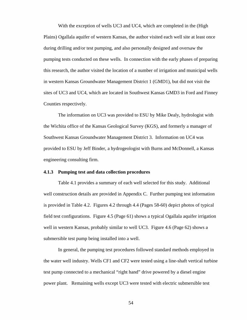
54
With the exception of wells UC3 and UC4, which are completed in the (High
Plains) Ogallala aquifer of western Kansas, the author visited each well site at least once
during drilling and/or test pumping, and also personally designed and oversaw the
pumping tests conducted on these wells. In connection with the early phases of preparing
this research, the author visited the location of a number of irrigation and municipal wells
in western Kansas Groundwater Management District 1 (GMD1), but did not visit the
sites of UC3 and UC4, which are located in Southwest Kansas GMD3 in Ford and Finney
Counties respectively.
The information on UC3 was provided to ESU by Mike Dealy, hydrologist with
the Wichita office of the Kansas Geological Survey (KGS), and formerly a manager of
Southwest Kansas Groundwater Management District 3. Information on UC4 was
provided to ESU by Jeff Binder, a hydrogeologist with Burns and McDonnell, a Kansas
engineering consulting firm.
4.1.3 Pumping test and data collection procedures
Table 4.1 provides a summary of each well selected for this study. Additional
well construction details are provided in Appendix C. Further pumping test information
is provided in Table 4.2. Figures 4.2 through 4.4 (Pages 58-60) depict photos of typical
field test configurations. Figure 4.5 (Page 61) shows a typical Ogallala aquifer irrigation
well in western Kansas, probably similar to well UC3. Figure 4.6 (Page 62) shows a
submersible test pump being installed into a well.
In general, the pumping test procedures followed standard methods employed in
the water well industry. Wells CF1 and CF2 were tested using a line-shaft vertical turbine
test pump connected to a mechanical “right hand” drive powered by a diesel engine
power plant. Remaining wells except UC3 were tested with electric submersible test
55
pumps, connected to a temporary power source and a temporary discharge line. Well
UC3 is a Ford County, Kansas irrigation well and was likely tested with its lineshaft
vertical turbine irrigation pump in place (see Figure 4.4 for a typical Ogallala / western
Kansas irrigation well), with temporary equipment installed to enable flow and water
level measurement. Well UC4 was installed in 1977 as a test-production well for a
proposed coal-fired generating plant and was likely tested with a lineshaft vertical turbine
test pump. Detailed presentation and analysis of the UC4 test data is provided in Burns
and McDonnell (1977) but the report lacks details on pumping test equipment and data
collection procedures.
In general, the discharge line for each tested well was equipped with at least one
valve used to control the flow, a flow measuring device, such as a flow meter or an
orifice tube (Figure 4.4), or an open discharge (in the case of the low yielding wells) that
facilitated direct measurement of discharge into a calibrated container using a stopwatch.
Water levels were measured using a temporary “sounding tube” placed inside the well
casing with the test pump. The sounding tubes provided a safe housing into which
electronic water level sensors were lowered. Some wells included two sounding tubes
(Figure 4.6), one housing a pressure transducer connected to a data logger and the other
for the electronic water level meter.
As is standard in the industry, water levels were measured in the wells prior to the
tests in order to establish the non-pumping water level, and in some cases, multiple
readings were made to ascertain any possible rising or falling water level trends. During
the pumping phase of the tests, water level and flow were recorded at high frequency
during the first 100 minutes of the test, and less frequently for the remainder of the tests.
The data sheets in Appendix A provide detailed information. Each test ran at a steady or
56
constant flow rate, generally not varying by more than 5% (often less). Several of the
tests followed the recovery period of variable – rate (step) tests performed prior to the
constant rate testing in order to assess well hydraulics and well specific capacity.
Following the cessation of pumping, the recovery of water levels was typically recorded
until full recovery occurred or until the rate of water level recovery as indicated on a
graph, was following a clear trend. According to Dealy (pers. comm 2011), the flow rate
of the 1979 test on UC3 was measured with a calibrated flow meter, and water levels
were measured with an air line.
The pumping test on UC4 included down-hole velocity surveys (spinner surveys),
used to identify specific production zones within a fairly long (160 ft) well screen
assembly. This data set is considered high quality: there were 13 readings of drawdown
in the first 60 minutes of the test, followed by hourly readings for the next 167 hours of
pumping at a rate of 2,000 gpm. See Appendix C for copies of relevant well construction
data.
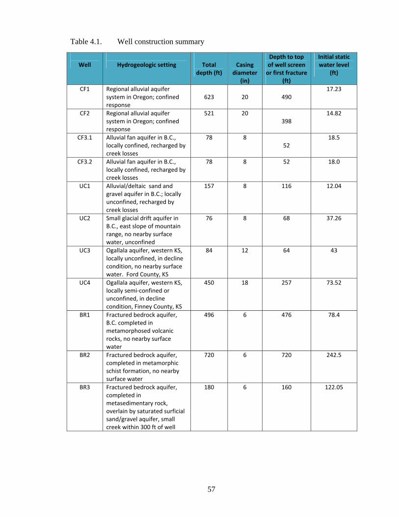
57
Table 4.1. Well construction summary
Well
Hydrogeologic setting Total
depth (ft) Casing
diameter (in)
Depth to top of well screen or first fracture
(ft)
Initial static water level
(ft)
CF1 Regional alluvial aquifer system in Oregon; confined response
623 20
490 17.23
CF2 Regional alluvial aquifer system in Oregon; confined response
521 20 398
14.82
CF3.1 Alluvial fan aquifer in B.C., locally confined, recharged by creek losses
78 8 52
18.5
CF3.2 Alluvial fan aquifer in B.C., locally confined, recharged by creek losses
78 8 52 18.0
UC1 Alluvial/deltaic sand and gravel aquifer in B.C.; locally unconfined, recharged by creek losses
157 8 116 12.04
UC2 Small glacial drift aquifer in B.C., east slope of mountain range, no nearby surface water, unconfined
76 8 68 37.26
UC3 Ogallala aquifer, western KS, locally unconfined, in decline condition, no nearby surface water. Ford County, KS
84 12 64 43
UC4 Ogallala aquifer, western KS, locally semi‐confined or unconfined, in decline condition, Finney County, KS
450 18 257 73.52
BR1 Fractured bedrock aquifer, B.C. completed in metamorphosed volcanic rocks, no nearby surface water
496 6 476 78.4
BR2 Fractured bedrock aquifer,completed in metamorphic schist formation, no nearby surface water
720 6 720 242.5
BR3 Fractured bedrock aquifer,completed in metasedimentary rock, overlain by saturated surficial sand/gravel aquifer, small creek within 300 ft of well
180 6 160 122.05

F
igure 4.2 Typical tes
arrow), sa
st well confi
mpling tap (
58
guration sho
(A), control v
A
owing well s
valve (B)
B
ounder, soun
Photo by
nding tube (
y author
(red

F
igure 4.3 Test pump
valve (C)
A
ping well hea
59
ad with well
B
sounder (A)), flow meter
C
Photo by
r (B) and con
y author
ntrol

F
igure 4.4 Flow meassurement usi
60
ing circular orifice platee and manom
Photo by
meter
y author

F
igure 4.5 Typical Hiigh Plains / O
61
Ogallala aquuifer irrigatioon well, Sco
Photo by
ott County, K
y author
KS

F
igure 4.6 Preparing
sounding
g submersibl
g tubes (arrow
62
le test pump
w)
for installat
Photo by autho
tion. Note d
or
dual PVC
63
4.1.4 Data set summaries
The following sections summarize the hydrogeologic setting and test conditions
for each of the eleven well test data sets from the ten wells used in this study. Because
many of the wells are public-water supply wells and the well owners may have concerns
around disclosure of specific well location information in external documents, the
specifics on the actual name or number of some wells and locations are purposefully
omitted. This excluded information is not critical to the central purpose of this study.
Copies of well logs and other pertinent information from the time of well construction are
provided in Appendix C.
The two Kansas High Plains Aquifer (Ogallala) wells (UC3 and UC4) included in
the study are identified as to location by conventional township, section and range
coordinates. Analysis of the pumping tests completed on these wells more than 30 years
ago coupled with current High Plains water level information enables examination of
well yield estimation methodologies in situations where an aquifer is in a decline
condition, thus providing an opportunity examine long-term mining yield utilizing
pumping test information. Because of its fairly extensive data set, proportionally more
detailed treatment is given to the UC4 data set, with further analysis on the implications
of these data provided in Chapter 6.
Wells CF1 and CF2
Wells CF1 and CF2 are high-capacity 20-inch diameter municipal production
wells completed within a confined to semi-confined alluvial aquifer. The wells are
screened within the third and deepest of three aquifers developed in the vicinity of the
production wellfield completed in a regionally extensive layered alluvial aquifer system.
The two wells are part of a large production wellfield that serves a metropolitan area and

64
has been extensively studied. A steady-state and transient-calibrated regional-scale
multi-layer numerical groundwater flow model exists for the aquifer system, with a
detailed model grid covering the vicinity of the production wells.
The CF1 and CF2 aquifer is hosted by an alluvial sand and gravel formation
interpreted to be fluvial in origin and is composed largely of sand and gravel that is
partially indurated, with calcium carbonate indicated to be the primary cementing agent.
The most productive zones within the aquifer are typically the non-cemented layers,
composed of clean medium-to coarse grained sand with minor gravel. Confining
pressure is such that the non-pumping (static) water level rises some 250 feet or more
above the top of the aquifer. The confining unit is composed of silt and clay, with inter-
bedded thin zones of water-bearing sand. At the location of Well CF1, the confining unit
behaves as an aquitard, and no leaky aquifer effects are notable in pumping tests
performed on wells completed in this part of the aquifer system. The location of well
CF2, about one mile to the east of CF1, is closer to the interpreted source of recharge to
the aquifer system (the aquifer and overlying aquitard are interpreted to sub-crop against
a saturated river channel deposit), and where the confining unit exhibits leaky aquitard
effects.
The author’s knowledge of well tests conducted in the general area of CF2
suggest a boundary condition response indicative of either recharge or leaky aquifer
effects. Because the top of the aquifer is shallower at CF2, however, there is less
available drawdown and consequently, well yields are generally lower. A poorly
understood negative boundary response was evident in the hydraulic response of
observation wells monitored during the CF1 pumping test.
65
For both tests, non-pumping water levels at the time of testing were generally
within 20 feet of ground surface and thus these wells had significant available drawdown
(HA). Both wells have long-string production assemblies consisting of approximately
100 feet of well screen, completed with an artificial sand pack in a sand-dominated
formation. Each well was test pumped by first conducting a four hour step test, followed
by a recovery period of approximately 24 hours, and then followed by a 1-2 day constant
rate pumping test and then recovery measurements. Nearby wells were not operating
during either of the pumping tests. During both tests, flow was measured with a
calibrated totalizing flow meter and water levels were monitored with pressure
transducers and manual water level meters using dual sounding tubes.
Well CF3
Well CF3 is an eight-inch diameter test-production well completed in a layered
alluvial fan aquifer system located in the interior region of British Columbia, Canada.
The aquifer at the well location is locally confined by a fine-grained silt and silty clay
layer found between the ground surface and the top of the aquifer. A wellfield is being
developed at the site to supply a planned fish hatchery operation. The well is located
approximately 100 feet from a perennial creek. The conceptual model of the aquifer is
that close to the apex of the alluvial fan (about 1 mile above the CF3 well site), the
alluvial sediments are thinner and in direct hydraulic communication with the creek. It is
in this upgradient location near the apex of the alluvial fan that the aquifer likely receives
considerable recharge through infiltrative creek bed losses.
At the CF3 site, the aquifer is composed of coarse-grained sand, with interbedded
fine gravel, and at the time of testing, the non-pumping static water level was within 20
feet of ground surface. CF3 was initially test pumped by conducting a step test, followed
66
by a recovery period and then a 48 hour constant rate pumping test at 350 gpm (data set
CF3.1). The following year, the well was test pumped again, this time at 145 gpm and
for 26 days (data set CF3.2). During both tests flow was recorded with an orifice and
manometer, and water levels were monitored with pressure transducers and manual water
level meters. A barometer transducer was also employed in order to enable correction of
the transducer data for atmospheric pressure variations.
Well UC1
Well UC1 is constructed similarly to CF3, but is completed in an unconfined
alluvial fan / deltaic sand and gravel aquifer, also in the interior region of British
Columbia, Canada. It is an 8-inch diameter well, constructed to supply a municipal water
supply system, and completed in a productive aquifer that has seen minimal historic
development (limited to two wells drilled for a park campground about 4,000 feet away).
The aquifer is recharged principally by infiltrative losses from a creek that passes
approximately 300 feet to the north of the well. A large valley-bottom lake is located 300
feet to the east of the well and is the natural discharge point for the alluvial aquifer. Well
UC1 was subjected to 670 minute constant-rate discharge test at 500 gpm (the well was
not tested longer due to the anticipated high capacity of the well relative to the yield
requirement of the well owner). Flow rate was measured using an orifice plate and
manometer (Figure 4.3). Water levels were measured with an electronic pressure
transducer and data logger and supplemented with manual water level readings collected
with electric well sounder using dual sounding tubes.
Well UC2
Well UC2 is a relatively shallow (76 ft) well screened in a small (less than 1 mi2)
stratified glacial drift aquifer system located in an upland area, composed of a large
67
terrace that fronts the eastern rampart of the Purcell Mountain Range in the Rocky
Mountains of British Columbia. The aquifer is of limited areal extent and was delineated
through a process of exploratory test drilling as its surface expression is minimal and
blends in with the surrounding landscape where only non-water-bearing glacial till and
moraine dominate the surficial geology. Due to the small size of the aquifer and the
relatively limited saturated thickness, Well UC2 was completed with just 8 feet of well
screen. Despite the apparent limited nature of the resource, the well was successfully
test-pumped for 72 hours at a constant rate of 159 gpm and exhibited strong recovery.
During the test, flow rate was measured with a totalizing flow meter, and water levels
were collected manually with an electric water level meter inserted into a single sounding
tube. Care was taken to discharge the test water at a considerable distance from the well,
to minimize short-circuiting of test water back into the aquifer during the test. No
evidence of short-circuiting (i.e. recharge) was noted.
Well UC3
UC3 is located in the NW 1/4 , SE ¼, NE ¼ of Section 17, Township 28S, Range
21W in Ford County Kansas. The well was chosen because of the quality of well test
documentation available: it was subjected to a 2.85-day (68-hr; 4,000 minute) constant
rate pumping test under the supervision of KGS staff in 1979 (Dealy and Jenkins 1980).
A plot of the pumping test data was used to generate time-drawdown data for use in this
study. Well UC3 is an irrigation well that was drilled in 1974 for the Ford Land and
Cattle Co. located near the community of Bucklin in Ford County, Kansas as few miles
west of the Ford and Kiowa county line, which forms the boundary between GMD5 and
GMD3. Groundwater resources in Ford County are presently managed by GMD3. The
UC3 well is completed in the unconfined Ogallala aquifer, which unconformably overlies

68
older bedrock units. Dealy and Jenkins (1980) noted that in Ford County, the
undifferentiated Pleistocene deposits may be in direct contact with the Tertiary Ogallala
Formation sediments, but where saturated, these units form a single aquifer. See
Appendix C for further well information obtained from the Dealy and Jenkins report. The
southeast Ford County area was noted by Dealy and Jenkins (1980) as having relatively
low aquifer saturated thickness and as of 1979 was declining at a rate of about 0.6 ft/year.
KGS maps indicate that the Ogallala aquifer saturated thickness in Haskell County (west
of Ford County) reaches 200 ft in some locations and exceeds 300 ft in parts of Finney
and Kearney counties further west (see UC4 description below for further discussion on
saturated thickness). The UC3 static water level at the time of the 1979 test was 43 feet
and at the well location, the Ogallala saturated thickness was a relatively thin 41 feet.
The current saturated thickness at the well site is not known but from nearby WIMAS
data, it is probably on the order of 27-29 feet, indicating a 12-14 ft decline since 1979.
Annual water level measurements at selected water level monitoring wells (KGS 2010) in
T28S R21W indicate a water level decline ranging between approximately 10 and 25 feet
near UC3 over the past 30 years, or approximately 0.3 to 0.8 ft per year.
Well UC4
UC4 is an 18-inch diameter production well located at a coal-fired power
generating plant located in Finney County a few miles west of Garden City near the
community of Holcomb, and like UC3 is within Southwest Kansas GMD3. UC4 is
located in the SW ¼ of Section 31, Township 24S, Range 33W and is completed within
one of the thicker portions of the Ogallala aquifer in western Kansas, and significantly
thicker than at UC3, which is located in an area where the predevelopment saturated
thickness was relatively small. However, groundwater declines over the past three

69
decades in Finney County near UC4 are considerably greater than in much of Ford
County. For a full discussion of changes in depth to water and saturated thickness in
GMD 3 refer to Macfarlane and Schneider (2007).
The well data set provided in the Burns and McDonnell (1977) report contains the
following data pertinent to this study:
Detailed well construction log for the test-production well;
Detailed formation (geologic) logs for the test borehole adjacent to the completed
well; and similar logs for several observation wells used during the pumping test;
Step-rate pumping test data for pumping at rates between 500 and 2,500 gpm on
UC4;
Constant rate pumping test data for pumping at rate of 2,000 gpm for 7 days,
followed by approximately 1 day of water level recovery measurement;
Graphical plots of pumping test data for the pumping well and observation wells;
and transmissivity estimates based on interpretation of the pumping test data;
Downhole velocity (spinner) survey data, collected during the step rate and
constant rate pumping tests; and
An electrical resistivity log, presumably conducted on the test hole prior to well
casing installation.
The saturated thickness (ST) of the Ogallala as defined by Macfarlane et al.
(2005) is the total thickness of saturated sediments between the water table (as measured
in the winter following an irrigation season) and the top of the bedrock surface. A
concept developed by Macfarlane and others at KGS, the practical saturated thickness
(PST) is a fraction of ST and represents only those layers identified as permeable and
productive, and is based on KGS staff interpretation of driller’s log formation
descriptions. At the time of its construction in 1977, the well exhibited a total Ogallala
ST of approximately 360 ft., whereas Macfarlane and Schneider (2007) estimated the pre-

70
development (ca. 1950) practical (permeable) saturated thickness (PST) of the Ogallala in
T24S, R33W in the range of 200 to 250 ft, and a 2006 PST of approximately 100 to 150
ft, with an overall PST/ST ratio of 50 to 75 percent.
The characteristic vertical stacking of contributing (water-bearing) and non-
contributing zones within the Ogallala hydrostratigraphic section has been observed
(Macfarlane and Schneider 2007) to produce a stair-step pattern of water level decline,
with higher decline rates occurring when the phreatic surface falls through non-
contributing zones and slower decline rates as the surface falls through permeable
contributing zones. Macfarlane’s method applies a defined set of “rules” that assign
logged formation materials as either non-contributing, 30% contributing, 70%
contributing, and 100% contributing, with complex mixtures assigned proportional PST
values based on the major and minor lithologies.
Recognizing the limitations of applying PST estimates based only on well log
information, Schulmeister and Geller (2009) developed an approach that uses downhole
spinner surveys and geophysical logs (similar to the tests conducted on UC4 in 1977) to
further refine the PST value at the scale of an individual well site. This technique could
serve as an alternative method to assess PST and long-term well yield when a formation
log is not available or is of poor quality, and could prove especially useful when
groundwater decline threatens high-value water supplies, for example, municipal supplies
or other individual water sources deemed important to the local economy.
The value of spinner logs is that they provide a direct measurement of
contributing and non-contributing zones, but can only be applied within the well screen
interval, so the productivity of the saturated Ogallala present above or below the well
screen cannot be assessed with this technique.
71
Combining spinner surveys with pumping tests increases the relative cost of
pumping tests, although the small diameter of some tools makes it possible to use them
without removing the well pump. In spite of the associated cost of well-specific testing
involving spinner surveys and other tools, the time may come when these become
necessary in order for well owners to make decisions about whether or not changes in the
well design could be made to optimize the ability of the source to extract groundwater
from a diminishing resource.
Appendix C contains the UC4 well log along with selected data from the original
pumping tests, the spinner surveys, and the electrical resistivity log. The spinner survey
and electric log data for UC4 suggest a PST value close to 50 percent of ST at this
location. According to the well diagram provided in the Burns and McDonnell (1977)
report, the UC4 screen assembly including blank sections spans approximately 180 feet
between depths 257 and 437 ft. The UC4 spinner data indicate relatively little production
was derived from the screen section below a depth of 370 ft. With the bottom of the well
screen at 437 ft, this suggests approximately 65 ft of low-producing Ogallala. There was
also relatively little contribution to the well from the upper 30 ft of screen between
approximately 257 and 290 ft. The latter suggests that the well pump could be lowered
by approximately 30 ft without compromising production from the intervals below. The
majority of the well production appeared to have been derived from the screen interval
between 295 and 370 ft, or about 45 percent of the 180 ft screen assembly interval. The
electrical resistivity log showed good correlation (i.e. high resistivity) with the well log
and zones of major inflow indicated on the spinner log, and also indicated a permeable
fraction of the Ogallala within the screen zone of about 50 percent.

72
Well drillers logs for the production well and three observation wells located
within 1,000 ft of UC4 interpreted using the technique of Macfarlane et al. (2005) also
suggest current PST (assuming a year 2010 depth to non-pumping water level of
approximately 175 ft) ranging from approximately 115 to 150 feet near UC4. If current
ST is approximately 260 ft, then the PST/ST ratio in the vicinity of UC4 likely ranges
from 45 to 58% with the most productive materials occurring in the approximate middle
of the remaining saturated Ogallala section.
In summary, based on a review of the data, it appears that the PST/ST fraction at
UC4 was approximately 50 percent when it was tested in 1977. A nearby annual water
level observation well (T24S, R33W, 34CAC), indicates a decline of approximately 100
ft since 1977, which would put the static water level at 175 ft, which is approximately 75
to 80 feet above the top of the well screen and 110 ft above the top of the main producing
zone. The 100 ft decline is likely affecting the long term capacity of UC4 and other
similar wells in GMD3 where large declines are evident. Such effects are further assessed
in Chapter 6.6. Figure 4.7 depicts the general well locations of the UC3 and UC4 as
related to 2003-2005 KGS-mapped saturated thickness of the Ogallala aquifer.
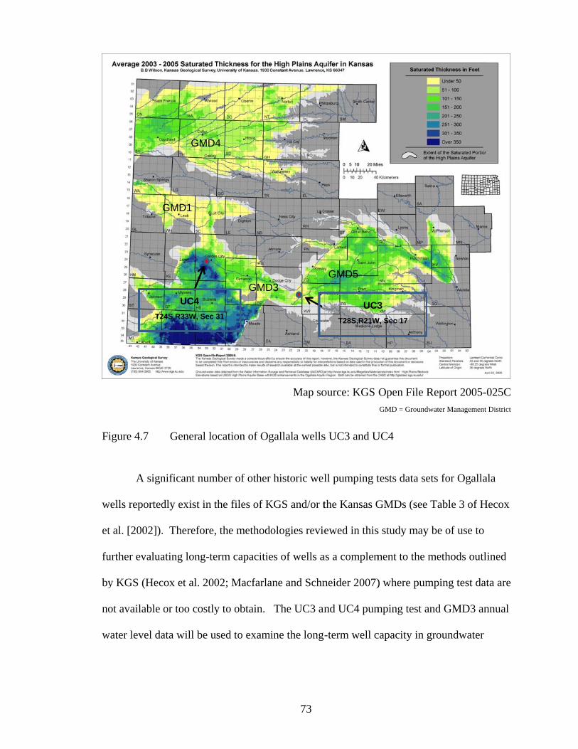
F
w
et
fu
by
no
w
igure 4.7
A sign
wells reported
t al. [2002]).
urther evalua
y KGS (Hec
ot available
water level da
T2
General lo
nificant num
dly exist in t
. Therefore,
ating long-te
cox et al. 200
or too costly
ata will be u
UC4
24S,R33W, Sec 3
GMD4
GMD1
ocation of Og
mber of other
the files of K
the method
erm capacitie
02; Macfarla
y to obtain.
sed to exam
31
4
GMD
73
Map so
gallala wells
r historic wel
KGS and/or t
ologies revie
es of wells a
ane and Schn
The UC3 an
ine the long-
D3
ource: KGS
s UC3 and U
ll pumping t
the Kansas G
ewed in this
as a complem
neider 2007)
nd UC4 pum
-term well c
UC3
T28S,R21W
GMD5
Open File R
GMD = Groundw
UC4
tests data set
GMDs (see T
s study may b
ment to the m
) where pum
mping test an
capacity in gr
3
W, Sec 17
Report 2005-
water Management
ts for Ogalla
Table 3 of H
be of use to
methods outl
mping test dat
nd GMD3 an
roundwater
025C
District
ala
Hecox
ined
ta are
nnual

74
decline situations (see Chapter 6.6). This analysis explores the concept of long-term
mining yield introduced in Chapter 2.
Well BR1
BR1 is a private domestic water well completed in a fractured bedrock aquifer
located in the interior of British Columbia, Canada. The well is approximately 500 feet
deep with an initial non-pumping static water level of 80 feet. As is typical of lower
yielding bedrock wells, the well driller estimated the well flow rate by conducting a short
airlift test using the drill rig. No water-bearing fracture information is provided on the
well log. On the basis of the driller’s estimated yield of 3 gpm, the well was test pumped
for 48 hours at a rate of 1.75 gpm. The flow rate was regulated with a control valve on the
discharge line and measured using the method of recording the time needed to fill a
container of known volume (the “bucket and stopwatch” method). The flow
measurements were made throughout the test at similar intervals to the water level
measurements, which were recorded using a manual electric water level meter inserted
into a single sounding tube.
Well BR2
BR2 is a proposed small community well source, completed in a deep fractured
bedrock aquifer situated along the margins of a large valley. The valley is filled with
relatively thick accumulations of glacial and alluvial sediment, while the adjoining
hillsides are mantled with a relatively thin veneer of glacial till, and underlain by
fractured bedrock. At a depth of 720 ft the deepest well used in this study, BR2 was test
pumped for 72 hours at a rate of 15 gpm. In the early minutes of the test, the flow rate
was initially 16.5 gpm and was then adjusted to 15 gpm. The flow rate was regulated
with a control valve on the discharge line, and water levels were measured with an

75
electric water level meter. Flow rate was measured with a magnetic flow meter; these
measurements were supplemented with periodic “bucket and stopwatch” readings. No
water-bearing fracture data are provided on the well log and so it is assumed that the
production is derived from the lower part of the borehole.
Well BR3
This well, at 180 ft, the shallowest of the three bedrock wells selected for this
analysis, is located in an upland setting, about halfway between the top of a broad
mountainous plateau and the Okanagan Valley bottom in the interior of British Columbia.
It is a proposed private domestic well and is situated within a proposed residential
subdivision comprised of lots ranging in size from approximately 2 to 5 acres, all
serviced by private wells. Although it has only about 35 feet of available drawdown, the
fractured formation appeared capable of supplying enough water to sustain flow rates of 1
to 2 gpm (the driller estimated 4 gpm based on an airlift test). The fractures are thought
to be steeply-dipping (i.e. vertical) and in hydraulic communication with an adjacent
saturated surficial formation composed of sand, silt and gravel. There is also a small
year-round creek passing through the area. BR3 was test pumped for 48 hours at a rate of
2.1 gpm. Flow rate was regulated with a control valve on the discharge line, and
measured with a calibrated bucket and stopwatch. Water levels were measured with an
electric water level meter inserted into a single well sounding tube.
Table 4.2 summarizes the pumping tests conducted on each of the ten wells
selected for the comparative analysis.

76
Table 4.2 Pumping test summaries
Well
Test flow rate (gpm)
Test duration (minutes)
Available drawdown
HA (ft)
Drawdown at end of test (ft)
1 hour specific capacity (Q/s;
gpm/ft)
CF1 3,520 2880 463 130.77 28.2
CF2 3,000 1680 375 103.79 29.2
CF3.1 350 2880 33 6.02 59.1
CF3.2 145 37000 33.5 3.6 63.0
UC1 500 670 67.3 9.65 50.0
UC2 159 4320 22.8 3.56 54.8
UC3 670 4050 27 10.0 67.0
UC4 2,000 10098 122.3 135 17.7
BR1 1.75 2880 407 193.51 .01
BR2 15 4320 467 186.0 .09
BR3 2.1 2880 48 21.09 .11
Note: HA for unconfined wells = 2/3 of total available drawdown
4.2 DATA PROCESSING AND ANALYSIS METHODS
In order to provide a suitable comparative analysis, each of the eleven well test
data sets was subjected to a consistent data processing and analytical procedure, which is
summarized below. The described sequence was followed in order to enable an initial
diagnostic step using the pressure derivative analysis, followed by calculation of aquifer
transmissivity and assignment of values needed to apply the Method A, B, and C
equations, calculation of LTWC, followed by assessment of sensitivity and other factors.
1. First, time, flow rate and water-level data were entered into two different
spreadsheets. The first spreadsheet was used to create standard hydrographs of
time versus drawdown and the drawdown versus the log of time (semi-log). This
spreadsheet provided three basic columns of data (plus the pumping rate): time,
depth to water, and drawdown, with depths in feet either to the nearest 0.01 or .1
feet depending on the data source. Then, these same data were copied and pasted
77
into the second ‘DERIV’ spreadsheet per the instructions for its use provided in
Allen (1999).
2. Second, the pressure derivative graph was created and interpreted for evidence of
radial flow (Theis-like) conditions. This test interval was then noted on the graph
by the analyst.
3. Based on the radial flow period (if one was identified), an estimate of aquifer
transmissivity was derived using mainly the Cooper-Jacob (1946) equation as
outlined in Chapter 4.1.
4. Any wells exhibiting non-radial flow response were flagged for further analysis
according to the appropriate analytical model, if one could be discerned in the
data. If not, the “best fit” analytical solution assuming Theis or Cooper-Jacob was
used, or a recovery analysis was done if sufficient recovery data were available.
5. For each well, input values for use in each of the three Long-Term Well Capacity
estimation spreadsheets were then culled from the data set (e.g. S, HA, S100, and
so on). If the later time drawdown trend formed a straight line on a semi-log plot
and could be explained by the general conceptual model, then this trend was used
to assign the S value.
6. Well capacity calculation spreadsheets were completed for each LTWC method,
and are summarized in the next Chapter.
7. Three specific-capacity ratios were calculated, as further described in Chapter
4.2.1 below.
8. A sensitivity analysis was done on the well capacity calculation worksheets as
summarized in Chapter 4.2.2 below.
9. Wells suspected or known to be influenced by external factors such as well
interference or groundwater decline were flagged for further analysis as described
in Chapter 6.
4.2.1 Specific capacity ratios
Three specific capacity ratios, an empirical technique developed by the author, are
proposed to aid in comparison of the well capacity calculation results, and to give an

78
indication of the temporal sensitivity of the calculated LTWC. These ratios are as
follows:
Ratio 1: is the Farvolden-method predicted 20 year specific capacity divided by
the actual one-day specific capacity.
Ratio 2: is the Moell-method predicted 20 year specific capacity divided by the
actual 100 minute specific capacity.
Ratio 3: is the CPCN-method predicted 100 day specific capacity divided by the
actual one-day specific capacity.
There is no way to directly relate aquifer transmissivity to well capacity. Because there is
a recognized empirical relationship between specific capacity and transmissivity (Driscoll
1986), the rationale for developing the specific capacity ratios is that the time-dependent
drawdown behavior of wells (which is a function of both transmissivity and pumping
rate) will be reflected by comparing a projected long-term specific capacity to a measured
short-term specific capacity. Except in the case of true equilibrium conditions, all wells
should have a specific capacity ratio less than 1.0. Wells with lower specific capacity
ratios experience a greater amount of drawdown per log cycle of time, and so capacity
calculations for such wells would tend to have greater temporal sensitivity.
Given the empirical relationship between pumping duration and drawdown in
non-equilibrium situations, it follows that for a particular LTWC analysis to be valid, the
specific capacity ratio should have a value less than 1.0 (i.e. the long-term drawdown is
greater than the shorter term drawdown at the same pumping rate). When this condition
(< 1.0 ratio) is not met, then this is a “flag” that the derived Q20 or Q100d value(s) may not
be valid, or indicative that further analysis is warranted.

79
4.2.2 Sensitivity analysis
In assessing groundwater problems where there are several variables, it is useful
to perform a sensitivity analysis to assess how a particular mathematical solution changes
when certain variables are systematically altered. For example, in groundwater flow
modeling assessments, assigned aquifer properties such as hydraulic conductivity are
typically varied in sensitivity analysis (Anderson and Woessner 1992). For pumping test
evaluations, while there are examples of sensitivity analysis on results from the literature
(Cobb, McElwee and Butt 1982), there are none for analyses of well capacity. However,
given the known relationships between pumping rate, pumping duration, and drawdown,
the pumping time (duration) for which a value of theoretical capacity is derived is
considered a significant factor and so this was varied for each method by one order of
magnitude of elapsed time. For example, the pumping time for the Method C (CPCN)
was varied by running the analysis for a 10-day and a 1,000-day projected drawdown. As
noted above, the specific capacity ratios were used as a starting point as indicators of the
relative temporal sensitivity of each well test result. The sensitivity of the variables in
each LTWC equation may also be demonstrated mathematically. The safety factor
changes the resulting LTWC by an amount that is in exact proportion to the change in the
safety factor; however, the magnitude of this change in terms of its effect on well
capacity depends on the characteristics of the well and the aquifer. Temporal effects due
to extending or reducing pumping time on calculated LTWC is more complex; the change
in the calculated value resulting from varying pumping time does not vary in exact
proportion to the change in pumping time.
For Method A (Farvolden), besides pumping time the only variable that could be
altered was the safety factor since it is arbitrarily assigned and could reasonably be higher
80
or lower. This was varied up and down by 0.1. For Method B (Moell) method, both the
safety factor (+/- 0.1) and the 100 minute drawdown value were varied in addition to
pumping time (increased and decreased by one order of magnitude). The 100 minute
drawdown used in the Moell formula was varied by +/- 10% as this field-measured value
could be subject to error caused by measurement inaccuracy or fluctuations in pumping
rate early in the test. For Method C (CPCN), in addition to the time of pumping the safety
factor was varied per the other methods.

81
CHAPTER 5
RESULTS
In this Chapter the principal findings of the investigation are presented including
the pumping test data interpretations, the calculations of aquifer properties, and the
resulting estimates of long term well capacity using the three principal methodologies.
Finally, the results and implications of the specific capacity ratios and sensitivity analysis
are presented.
5.1 PUMPING TEST INTERPRETATION
Pumping test data tables, hydrographs, derivative plots and aquifer parameter
estimations are provided in Appendix A. Table 5.1 summarizes the interpreted results of
the pumping test data, including the assessment of the pressure derivative, the drawdown
response (either semi-logarithmic or logarithmic), and the estimated aquifer
transmissivity (and method[s] employed).

82
Table 5.1 Aquifer Test Interpretation Summary
Well test data set
Pressure derivative:
apparent time interval of radial flow (minutes)
Observed drawdown response
Estimated transmissivity T in gpd/ft and ft2/day
Method(s) used to estimate T
CF1 10‐1000 Flat derivative middle of test, late time negative
boundary effect
42,200 / 5,600 Cooper‐Jacob; Theis
CF2 5‐800 Declining derivative; late time recharge effect
49,000 / 6,500 Cooper‐Jacob
CF3.1 10‐300 Mostly flat derivative; straight line on semi‐log
84,000 / 11,200 Cooper‐Jacob
CF3.2 10‐2300 Barrier boundary evident after ~2600 minutes
95,000 / 12,800 Cooper‐Jacob
UC1 10‐80? Apparent short period of radial flow
330,000 / 44,000 Cooper‐Jacob
UC2 15‐500 Apparent negative boundary at ~500 minutes
38,000 / 5,000 Cooper‐Jacob
UC31 10‐4000 Mostly flat derivative 160,000 / 21,300 1979 T value per Dealy and Jenkins 1980 (used Cooper‐
Jacob)
UC42 30‐1300 Mostly flat derivative, with rising derivative in late time (possible variable
pumping rate)
45,000 / 6,000 1977 T value per Burns and McDonnell report (used Cooper‐
Jacob)
BR1 100‐800 Radial flow after early borehole storage effects
5.4 / 0.71 Cooper‐Jacob
BR2 70‐2000+ Radial flow after early borehole storage effects
115 / 15.3 Cooper‐Jacob
BR3 100‐2000+ Radial flow after early borehole storage effects
37.0 / 4.9 Cooper‐Jacob
Notes: 1. Year 2010 effective transmissivity is less due to groundwater decline of approximately 14 feet; see Chapter
6.6. 2. Year 2010 effective transmissivity is less due to groundwater decline of approximately 100 ft; see Chapter
6.6. 3. + denotes radial flow may have continued beyond the value given, but this is uncertain due to end effects 4. ? denotes that radial flow may have lasted slightly less or more than the time interval indicated.
5.2 LONG TERM WELL CAPACITY RESULTS
Tables 5.2 through 5.4 provide the summary long term well capacity calculations
for the three principal methods assessed in this study. Each table shows the basic input
data and also provides predicted and actual specific capacity values and the respective

83
specific capacity ratio (i.e. Ratio 1, 2 or 3). Table 5.5 provides a comparative view of the
results for all three of the methods. Refer to Chapter 3 for explanation of the variables
HA, Qt, 8S and S.
Table 5.2 Method A (Farvolden) well capacity estimation results
Boxed cells in red show specific capacity ratio value > 1.0 indicating invalid result
HA = available drawdown (ft)
S = change in drawdown in one log cycle of time (ft)
Well # Test flow rate HA
static water
level
water level
end of test
drawdown per log
cycle of time 8 S
Predicted 20 year
specific capacity
Q/s Q20
Actual 1 day
specific
capacity Q/s
Ratio 1: 20 year
to 1 day specific
capacity
(gpm) (ft) (ft) (ft) S (ft) (ft) (gpm/ft) (gpm) (gpm/ft)
CF1 3,520 463 17.23 148 22 176 20.0 6,482 28.2 0.71
CF2 3,046 375 14.82 118.61 16.5 132 23.1 6,057 29.2 0.79
CF3.1 350 33 18.5 24.62 0.6 4.8 72.9 1,684 59.1 1.23
CF3.2 145 33.5 18 21.6 0.6 4.8 30.2 708 63 0.48
UC1 500 67.3 12.04 21.69 0.4 3.2 156.3 7,361 50 3.13
UC2 159 22.8 33.7 37.26 2.2 17.6 9.0 144 54.8 0.16
UC3 670 27 43 53 1.2 9.6 69.8 1319 67 1.04
UC4 2,000 122.3 73.52 208.6 11.7 93.6 21.37 1,829 15.6 1.37
BR1 1.75 407 78.4 271.91 85.5 684 2.56E‐03 0.73 0.01 0.26
BR2 15 467 242.5 428.5 45 360 4.17E‐02 13.62 0.09 0.46
BR3 2.1 48 122.05 143.14 15 120 1.75E‐02 0.59 0.11 0.16
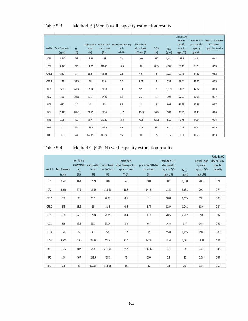
84
Table 5.3 Method B (Moell) well capacity estimation results
Table 5.4 Method C (CPCN) well capacity estimation results
Well # Test flow rate HA
static water
level
water level
end of test
drawdown per log
cycle
100 minute
drawdown 5 S Q20
Actual 100
minute
specific
capacity
Predicted 20
year specific
capacity
Ratio 2: 20 year to
100 minute
specific capacity
(gpm) (ft) (ft) (ft) S (ft) S100 min (ft) (ft) (gpm) (gpm/ft) (gpm/ft)
CF1 3,520 463 17.23 148 22 100 110 5,433 35.2 16.8 0.48
CF2 3,046 375 14.82 118.61 16.5 92 82.5 4,582 33.11 17.5 0.53
CF3.1 350 33 18.5 24.62 0.6 4.9 3 1,023 71.43 44.30 0.62
CF3.2 145 33.5 18 21.6 0.6 1.64 3 733 88.41 31.25 0.35
UC1 500 67.3 12.04 21.69 0.4 9.9 2 1,979 50.51 42.02 0.83
UC2 159 22.8 33.7 37.26 2.2 2.2 11 192 72.27 12.05 0.17
UC3 670 27 43 53 1.2 8 6 905 83.75 47.86 0.57
UC4 2,000 122.3 73.52 208.6 11.7 115.67 58.5 983 17.29 11.48 0.66
BR1 1.75 407 78.4 271.91 85.5 71.6 427.5 1.00 0.02 0.00 0.14
BR2 15 467 242.5 428.5 45 120 225 14.21 0.13 0.04 0.35
BR3 2.1 48 122.05 143.14 15 11 75 0.82 0.19 0.02 0.13
Well # Test flow rate
available
drawdown
HA
static water
level
water level
end of test
projected
drawdown per log
cycle of time
projected 100 day
drawdown
Predicted 100‐
day specific
capacity Q/s Q100
Actual 1 day
specific
capacity Q/s
Ratio 3: 100
day to 1 day
specific
capacity
(gpm) (ft) (ft) (ft) S (ft) (ft) (gpm/ft) (gpm) (gpm/ft)
CF1 3,520 463 17.23 148 22 180 20.1 6,338 28.2 0.71
CF2 3,046 375 14.82 118.61 16.5 141.5 21.5 5,651 29.2 0.74
CF3.1 350 33 18.5 24.62 0.6 7 50.0 1,155 59.1 0.85
CF3.2 145 33.5 18 21.6 0.6 2.74 52.9 1,241 63.0 0.84
UC1 500 67.3 12.04 21.69 0.4 10.3 48.5 2,287 50 0.97
UC2 159 22.8 33.7 37.26 2.2 6.4 24.8 397 54.8 0.45
UC3 670 27 43 53 1.2 12 55.8 1,055 69.8 0.80
UC4 2,000 122.3 73.52 208.6 11.7 147.5 13.6 1,161 15.56 0.87
BR1 1.75 407 78.4 271.91 85.5 361.6 0.0 1.4 0.01 0.48
BR2 15 467 242.5 428.5 45 250 0.1 20 0.09 0.67
BR3 2.1 48 122.05 143.14 15 35 0.1 2.0 0.11 0.55

85
Table 5.5 Comparison of all methodologies results
Boxed cells with red values indicate Ratio 1 being greater than 1.0, which means Q20 values are likely over-predicted by Method A.
As indicated in Tables 5.1 to 5.4, the wells selected for this study exhibit a range
of transmissivities, LTWC values, and specific capacity ratios. Regarding the ratios,
there are three groupings of wells: those with lower specific capacity ratios (i.e. less than
0.50), wells with generally higher specific capacity ratios (> 0.50) and one well (UC1)
with high Ratio 2 and 3 values that approach unity. The Farvolden method ratios (Ratio
1, shown in boxed cells with red numbers in Table 5.5) help explain the high LTWC
values for these four wells, which are considered significant over-predictions. The higher
the Ratio 1 values indicate a strong under-prediction of early time drawdown and an
over-prediction of Q20.
Well # Test flow rate
Method A
Q20
(Farvolden)
Method B
Q20 (Moell)
Method C
Q100
(CPCN) Ratio 1 Ratio 2 Ratio 3 Remarks(gpm)
CF1 3,520 6,482 5,433 6,338 0.71 0.48 0.71
CF2 3,046 6,057 4,582 5,651 0.8 0.5 0.74
CF3.1 350 1,684 1,023 1,155 1.23 0.62 0.85 Farvolden over‐predicts
CF3.2 145 708 733 1,241 0.48 0.35 0.84
UC1 500 7,361 1,979 2,287 3.13 0.83 0.97 Farvolden over‐predicts
UC2 159 144 192 397 0.16 0.17 0.45 100 day capacity>> 20 yr
UC3 670 1,319 905 1,055 1.04 0.57 0.80 Farvolden over‐predicts
UC4 2,000 1,829 983 1,161 1.37 0.66 0.87 Farvolden over‐predicts
BR1 1.75 0.73 1.00 1.4 0.26 0.14 0.48
BR2 15 13.62 14.21 19.6 0.46 0.35 0.67
BR3 2.1 0.59 0.82 2.0 0.16 0.13 0.55
Method A Farvolden appears
to be conservative in low‐
yielding bedrock wells. Also
note that 100 day capacity is
greater than the Q20
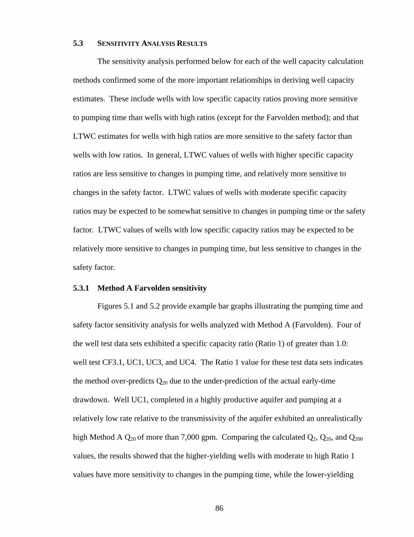
86
5.3 SENSITIVITY ANALYSIS RESULTS
The sensitivity analysis performed below for each of the well capacity calculation
methods confirmed some of the more important relationships in deriving well capacity
estimates. These include wells with low specific capacity ratios proving more sensitive
to pumping time than wells with high ratios (except for the Farvolden method); and that
LTWC estimates for wells with high ratios are more sensitive to the safety factor than
wells with low ratios. In general, LTWC values of wells with higher specific capacity
ratios are less sensitive to changes in pumping time, and relatively more sensitive to
changes in the safety factor. LTWC values of wells with moderate specific capacity
ratios may be expected to be somewhat sensitive to changes in pumping time or the safety
factor. LTWC values of wells with low specific capacity ratios may be expected to be
relatively more sensitive to changes in pumping time, but less sensitive to changes in the
safety factor.
5.3.1 Method A Farvolden sensitivity
Figures 5.1 and 5.2 provide example bar graphs illustrating the pumping time and
safety factor sensitivity analysis for wells analyzed with Method A (Farvolden). Four of
the well test data sets exhibited a specific capacity ratio (Ratio 1) of greater than 1.0:
well test CF3.1, UC1, UC3, and UC4. The Ratio 1 value for these test data sets indicates
the method over-predicts Q20 due to the under-prediction of the actual early-time
drawdown. Well UC1, completed in a highly productive aquifer and pumping at a
relatively low rate relative to the transmissivity of the aquifer exhibited an unrealistically
high Method A Q20 of more than 7,000 gpm. Comparing the calculated Q2, Q20, and Q200
values, the results showed that the higher-yielding wells with moderate to high Ratio 1
values have more sensitivity to changes in the pumping time, while the lower-yielding

be
ti
ti
of
sa
0
m
sa
edrock well
me – princip
me drawdow
f drawdown
ame general
.8 as compar
most wells, v
ame amount
Q20 values w
pally becaus
wn in low-yi
from casing
pattern is se
red to the de
arying the Q
(about 15%
were much l
e the Farvol
ielding bedro
g storage effe
een in the sen
efault 0.7 val
Q20 safety fac
%) as when pu
87
ess sensitive
den method
ock wells. T
fects during t
nsitivity ana
lue. As indi
ctor by 0.1 c
umping time
e to decrease
does not ten
This may be
the earlier pa
alysis run wi
icated by the
changed the L
e was varied
es or increas
nd to under-p
due to the re
art of the pum
ith safety fac
e arrows in F
LTWC value
d by one orde
es in pumpin
predict early
elatively low
mping test. T
ctors of 0.6 a
Figure 5.2, fo
e by about th
er of magnitu
ng
y-
w rate
The
and
or
he
ude.
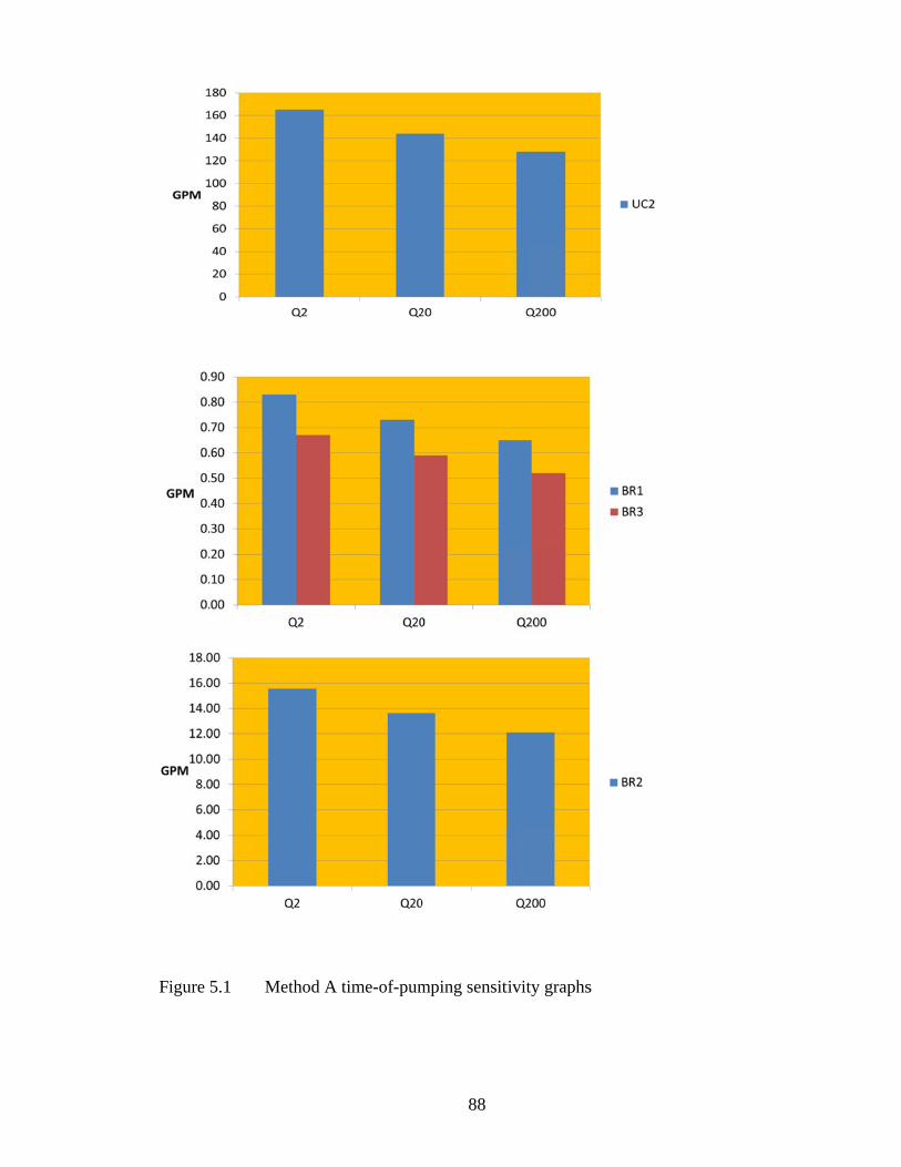
F
igure 5.1 Method A time-of-pum
88
mping sensittivity graphs
s
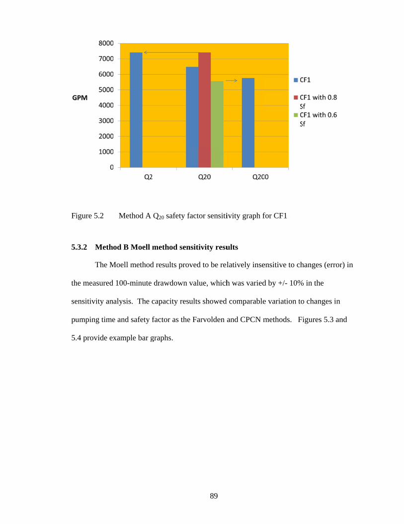
F
5
th
se
pu
5
igure 5.2
.3.2 Meth
The M
he measured
ensitivity an
umping time
.4 provide ex
Method A
od B Moell
Moell method
100-minute
alysis. The
e and safety
xample bar g
Q20 safety f
method sen
d results pro
e drawdown
capacity res
factor as the
graphs.
89
factor sensiti
nsitivity resu
ved to be rel
value, which
ults showed
e Farvolden
ivity graph f
ults
latively inse
h was varied
d comparable
and CPCN m
for CF1
ensitive to ch
d by +/- 10%
e variation to
methods. F
hanges (error
% in the
o changes in
igures 5.3 an
r) in
n
nd
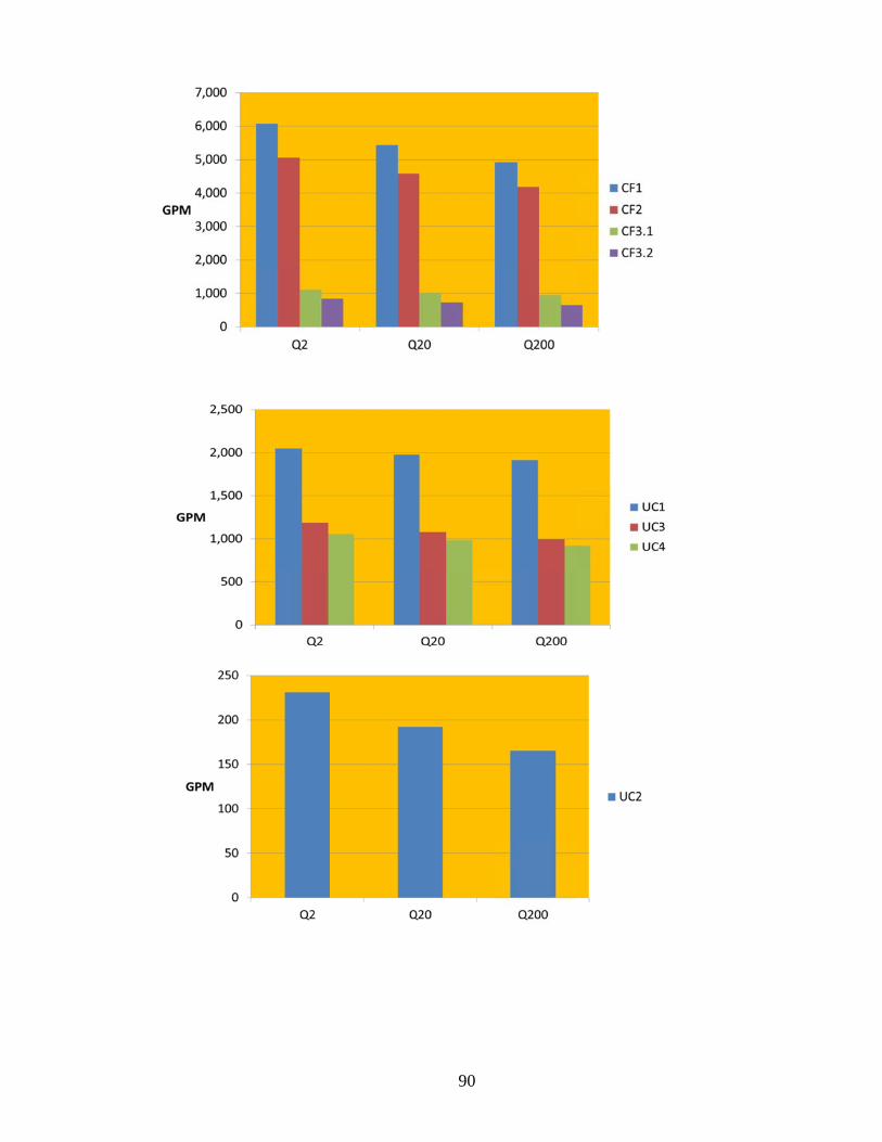
90
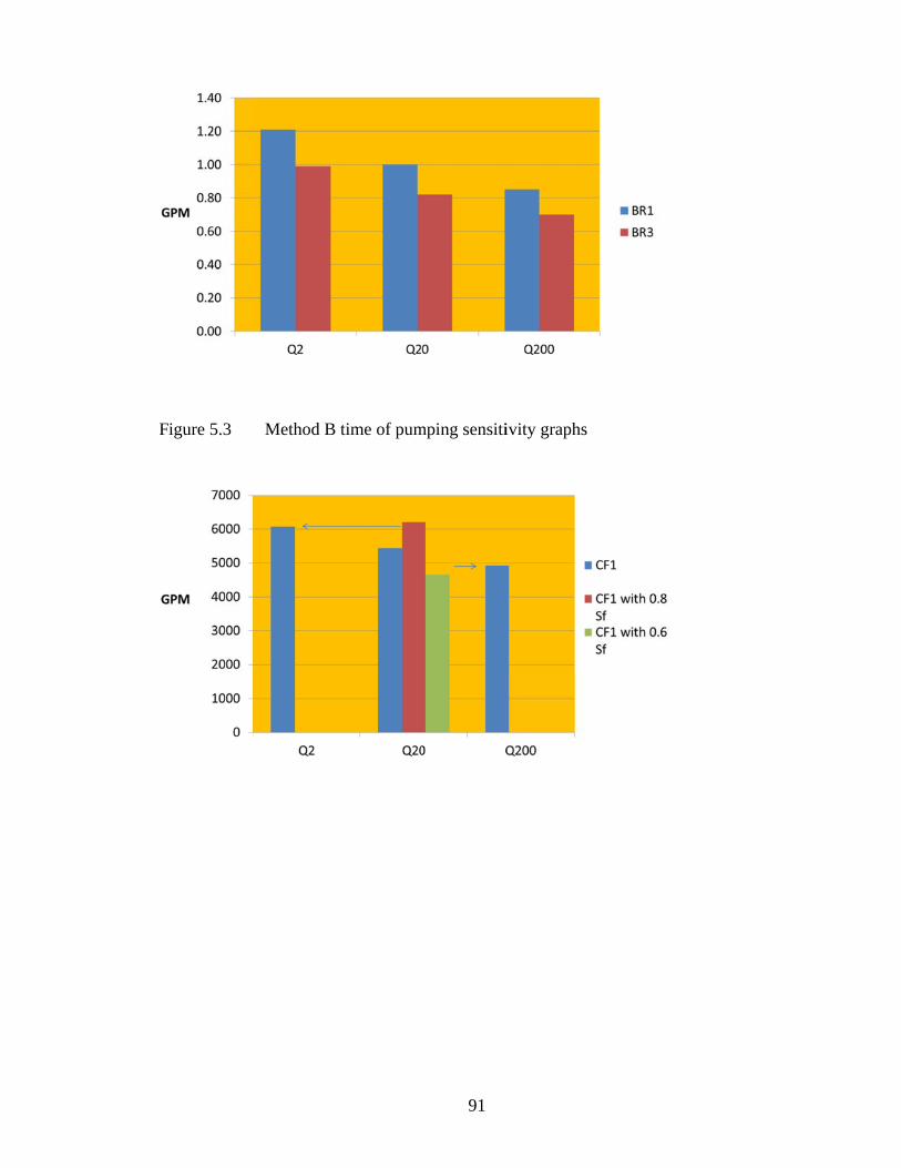
F
igure 5.3 Method B time of pum
91
mping sensitiivity graphs

F
W
th
by
sa
de
ca
th
M
m
5
ad
M
igure 5.4
Well CF1 had
he pumping t
y adjusting t
Well U
afety factor h
ecreasing pu
apacity ratio
he formula.
Moell method
most cases.
.3.3 Meth
The sa
djustment, a
Method C. A
Method B
d a moderate
time provide
the safety fac
UC1 had a h
has a more p
umping time
o, the more s
Interestingly
d sensitivity
od C CPCN
ame general
and Q20 sensi
As expected,
Q20 safety f
e Ratio 2 val
es estimated
ctor in the Q
high Ratio 2
pronounced e
. This analy
ensitive the
y, a 10% erro
analysis doe
N sensitivity
relationship
itivity observ
there were r
92
factor sensiti
lue of 0.48 a
yield values
Q20 formula b
value (0.83)
effect on the
ysis shows th
Q20 result w
or in the 100
es not appea
results
ps between s
ved for Meth
relatively sig
ivity graph f
and a one ord
s that are qu
by 0.1.
) and conseq
e Q20 value c
hat in genera
would be to th
0 minute dra
ar to significa
specific capa
hod B was ev
gnificant diff
for CF1 and
der of magni
uite similar to
quently, the a
compared to
al, the higher
he safety fac
awdown as v
antly affect t
acity ratios, s
vident in the
fferences in t
UC1
itude change
o values obta
adjustment o
increasing o
r the specific
ctor applied
varied for the
the results in
safety factor
e results for
the well
e in
ained
of the
or
c
in
e
n
r

ca
1
pu
se
pr
apacities det
,000-day cap
umping and
een for the M
rovides exam
termined for
pacity of We
safety facto
Method B M
mple bar gra
r the 10-day
ell CF1 was
or sensitivity
oell analyse
aphs for the t
93
and 1,000-d
20% less tha
results follo
s (see 5.3.4 b
time of pump
day sensitivit
an the 10-da
owed the sam
below for a
ping sensitiv
ty runs. For
ay value. Ov
me pattern of
summary).
vity.
example, th
verall, the tim
f variation a
Figure 5.5
he
me of
as
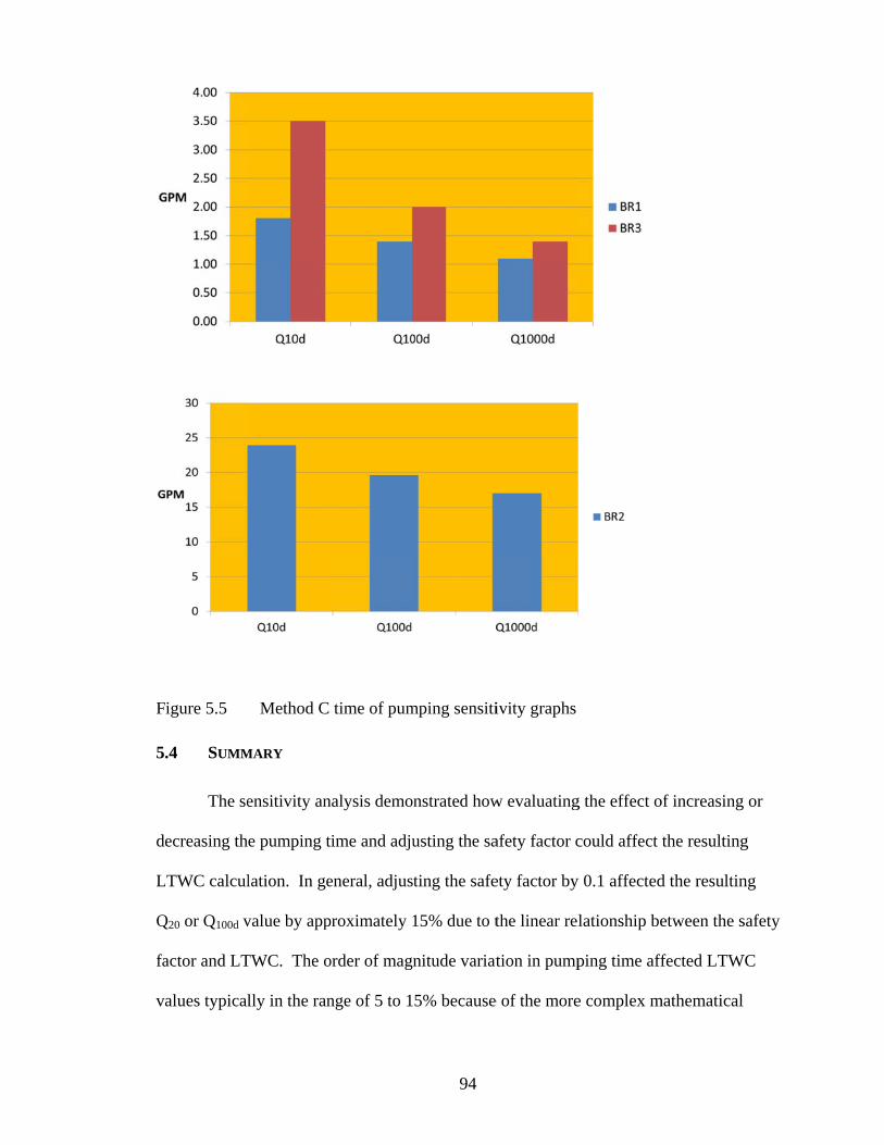
F
5
de
L
Q
fa
va
igure 5.5
.4 SUMM
The se
ecreasing th
LTWC calcul
Q20 or Q100d v
actor and LT
alues typical
Method C
MARY
ensitivity an
e pumping t
lation. In ge
value by app
TWC. The o
lly in the ran
time of pum
nalysis demon
ime and adju
eneral, adjus
proximately 1
order of magn
nge of 5 to 1
94
mping sensiti
nstrated how
usting the sa
ting the safe
15% due to t
nitude variat
5% because
ivity graphs
w evaluating
afety factor c
ety factor by
the linear rel
tion in pump
e of the more
g the effect o
could affect
y 0.1 affected
lationship be
ping time aff
e complex m
of increasing
the resulting
d the resultin
etween the s
ffected LTW
mathematical
or
g
ng
safety
WC
95
relationship between pumping time and well capacity: when S is small, then the Q20
or Q100d will also be small when pumping time is varied.
In cases where there is uncertainty about long-term recharge to the aquifer, or
possible future well interference, it could be advisable to adjust the safety factor to 0.6 or
even 0.5 in a Q20 analysis. For Method C, which calculates a single peak season well
yield for 100 days of pumping, the pumping time may be extended one order of
magnitude to provide a three-year well capacity (1000 days), which would be one way to
plan for a drought scenario.
Pumping test data sets combined with the application of the long-term well
capacity analyses provides an easy way to calculate the well’s specific capacity ratio.
The ratios assigned for the 10 well test data sets showed how the Farvolden method could
lead to over or under-predicted Q20 values, whereas the Moell and CPCN methods were
generally deemed reliable and each data set exhibited a consistent pattern in changes to
LTWC estimates in the sensitivity analysis, indicating that these methods may be used
reliably. Maathuis and van der Kamp (2006) recommended that use of the Farvolden
method be discontinued, which seems reasonable given that the Moell method is just as
easy to apply. In a Q20 LTWC calculation using Method B (Moell), if the 100 minute
drawdown data point is not available, or cannot be reasonably interpolated from test data,
then a safety factor of 0.5 or 0.6 should be considered for wells analyzed with the
Farvolden method.
For all three methods, LTWC estimates sometimes surpassed the test pumping
rate and/or the practical limit of production due to the well diameter, and for UC1, CF1,
CF2 and CF3 the exceedance was by a considerable amount. In the case of the three
confined aquifer wells, well interference factors into the actual LTWC and is discussed

96
further in Chapter 6. The CPCN method states that the calculated Q100d not exceed the
test pumping rate unless sufficient justification is provided by the hydrogeologist.
Similarly, the State of Vermont (2010) water supply rules only allow for a 10% upward
adjustment in the safe well yield (provided justification is given in the hydrogeologic
report). Such limitations are well-advised, because the LTWC analysis already
extrapolates relatively short-term pumping tests to long term pumping scenarios.
Assigning a higher pumping rate based on this extrapolation could lead to unforeseen
problems. The determination of a high theoretical Q100d or Q20 is useful in that the result
may indicate that a larger well, or a higher rate pumping test, or both, may be feasible to
assess the resource further.

97
CHAPTER 6
DISCUSSION ON SELECTED TECHNICAL ISSUES
The foregoing analysis of LTWC focused on evaluating yield from an individual
well over a specified time period, giving consideration to well and aquifer hydraulics, but
with minimal consideration of outside factors. There are a number of these potentially
complicating factors that may need to be considered during the process of assigning a
value of “well yield”, which could serve to further constrain the derived value, and
provide a means to predict how well yield may change with the dynamics of the well-
aquifer system. Some of these issues may be accounted for by using professional
judgement and applying a more conservative safety factor as noted above. Other
situations would likely require further assessment. The following sections highlight some
of the more important considerations and provide further assessment using some of the
well test data sets to help illustrate the potential significance of these issues.
6.1 WELL CONSTRUCTION FACTORS INFLUENCING LONG TERM CAPACITY
Conventional aquifer test analysis usually assumes that wells are “fully
penetrating”, that is, they are open to the entire saturated thickness of the aquifer. In
practice, this is rarely the case in unconfined aquifers, and even in confined aquifers with
high piezometric heads, it is usually not necessary to screen the entire aquifer thickness in
order to develop a successful production well. In fact, placing the well screen or open
interval as deep as possible is usually good practice, as it allows for additional available
drawdown.

98
Driscoll (1986) noted that well casing diameter is more important than screen diameter
when it comes to constraints on well yield, because casing diameter limits the size and
capacity of well pumps.
For wells completed with screens in unconsolidated formations, well development
is critical to long-term well yield. If development is not completed, then well
performance is likely to decline. The resulting loss of specific capacity has a direct
impact on the long-term well capacity.
Well screen transmitting capacity is sometimes stated as a limiting factor to well
yield by hydrogeologists, engineers and water well drillers. When radially flowing
groundwater approaches a well, its velocity (actually the specific discharge) increases
(Williams 1981). If velocity exceeds a critical value, head losses could occur as the water
passes through the screen and/or if turbulent flow occurs. The concepts of entrance and
approach velocity and head losses as they relate to well design are discussed in
Rorabaugh (1953) Williams (1981), and Driscoll (1986), among other papers. The basic
theory is that as water is drawn into a well screen from the formation, the increased head
difference between the formation and the pumping water level in the well causes the
velocity of the flow to increase. This velocity further increases as water passes through
the well screen openings. When the flow reaches a critical velocity, it may become
turbulent, which leads to further well losses (greater drawdown) and over the long term
may contribute to deteriorating well performance. Rorabaugh (1953) found that turbulent
flow due to over-pumping effects may have a dramatic effect on increasing well
drawdown.
As Williams (1981) noted, a high approach or entrance velocity may mobilize fine
formation sediment toward the well screen, contributing to plugging of the screen and

99
adjacent formation. For wells completed with well screens it is advisable to review the
screen transmitting capacity and consider this theoretical value in assigning an
appropriate long-term well capacity.
6.2 SEASONAL OR ANNUAL WATER LEVEL FLUCTUATION
Seasonal and annual patterns of groundwater level variation should be understood,
either through direct observation well data or through analysis of available regional data,
when assessing long-term well yield. If a given well is test-pumped during the normal
period of high water levels, and it is intended to be operated primarily at times of low
water levels, this information must be factored into the final assessment of long-term well
capacity by adjusting the available drawdown (HA) term. When possible, wells should be
tested and evaluated against low water conditions in order to derive a conservative
estimate of long-term well capacity. Then, a higher operating capacity can be assigned
for certain pumping periods that coincide with normally higher groundwater levels.
6.3 FACTORING IN CHANGES IN WELL PERFORMANCE (SPECIFIC CAPACITY)
The CPCN Guidelines (Allen et al. 1999) list changes in well performance as one
of the issues that could be addressed through the application of the recommended 0.7
safety factor. However, in cases where there is good evidence that production well
performance declines are common, a site-specific well performance factor should be
considered in assessing long-term well yield. This requires professional judgement, and a
subjective “de-rating” of the calculated well capacity that is intended to reduce the
operational pumping rate, and possibly delay the onset of well performance problems.
6.4 PUMP PERFORMANCE CONSIDERATIONS
In assessing long-term well capacity, the hydrogeologist may need to consider
pump design and performance issues, and make appropriate recommendations that take

100
these issues into consideration. These issues are normally beyond the scope or control of
a hydrogeological assessment, and involve engineering and economic factors. The recent
paper by Konikow (2010) discusses some of the more important concepts, such as the
fact that most well pump motors operate at a single speed, which means the flow rate
changes as drawdown in the well increases. With most wells being assigned a single,
fixed “safe” yield, well owners need to be able to properly plan for the effects of long-
term pumping on well production rates. Variable speed pumps combined with flow
control valves are an attainable way to engineer a steady flow rate from wells. The main
issues to consider are whether or not the well has a low specific-capacity ratio and if so,
then if the well pump to be used is a constant-speed, then the long-term flow rate of the
well decreases as drawdown increases. Variable speed pumps can maintain a steady flow
rate under a much broader range of water level conditions, and in some cases may be
needed to enable a predictable flow rate.
As noted above, well casing diameter generally limits the size pump that can be
installed in wells. Driscoll (1986) provides some guidelines on the typical practical
maximum yield of wells based on diameter. As a further example, Well CF1, although it
has a theoretical yield of more than 4,000 gpm, is limited to approximately 3,500 gpm
because it is a 20-inch diameter well. A similarly-constructed 24-inch diameter well at
the location of CF1 could potentially yield more than 4,000 gpm.
6.5 INVESTIGATION OF WELL INTERFERENCE EFFECTS
Well interference must be accounted for when measurable drawdown occurs
during the simultaneous operation of wells. In terms of the effect on calculating well
capacity, well interference reduces the available drawdown (HA value). If well
interference represents only a small percentage of HA, then the default 0.7 safety factor
101
may be sufficient to account for the effect of interference. If well interference is larger,
then either the HA value or the safety factor requires adjustment, and the resulting
estimate of well capacity should be less than the theoretical value derived on the basis of
the pumping test. Application of the R20 concept as proposed by Maathuis and van der
Kamp (2006) is one way to address well interference, and this may be done with or
without observation well time-drawdown data.
This section presents the results of applying a well interference factor to the well
capacity estimation method for two of the wells: CF1 and CF2. Operation of other wells
completed in the same aquifer causes approximately 100 ft of drawdown in each of these
wells. For this analysis, an additional 100 ft of drawdown attributed to well interference
is factored into the well capacity estimation spreadsheets. This is easily accounted for in
the calculation spreadsheets by reducing the HA value by 100 ft. Table 6.1 summarizes
the resulting Q20 and Q100d values calculated for these two wells. It is evident that
factoring interference could have a significant effect on the resulting well capacity
calculation and the magnitude of the effect is similar for each of the three methods, with
the greatest reduction in capacity seen in the Farvolden method.

102
Table 6.1 Analysis of Wells CF1 and CF2 well interference effects
Scenario Well CF1 LTWC (gpm) Well CF2 LTWC (gpm)
Method A no interference 6,482 6,057
Method A with 100 ft of
well interference
5,082 4,442
Difference 1,400 1,615
Method B no interference 5,433 4,582
Method B with 100 ft of
interference
4,259 3,360
Difference 1,174 1,222
Method C no interference 6,338 5,651
Method C with 100 ft of
interference
4,969 4,144
Difference 1,369 1,507
6.6 INVESTIGATION OF LONG TERM MINING YIELD
This section assesses how the loss of saturated thickness, i.e. groundwater decline
affects the theoretical long-term capacity of wells completed in the Ogallala aquifer in
Kansas, using the two example wells evaluated in this study located in GMD3. First, a
simple analysis based only on water level changes will be presented. Then, the effect of
reduced aquifer transmissivity will be investigated in order to illustrate the potential
decline in well yields between when they were originally tested and the present-day, and
the implications for expected reduction in well capacity that could occur over the next 20
years. These results are then compared to the findings of Hecox et al. (2002), which
presented KGS’ area-wide assessment of the relationship between well yield and
saturated thickness in the Ogallala aquifer.

103
6.6.1 LTMY of UC3 and UC4 using current HA
Focusing on the two Q20 methods, this exercise started with the 1977 and 1979
pumping test data, then factored in current (2010) water level observation data (KGS
2010) to calculate an estimated current HA value, and then assumed a continued trend of
decline for the next 20 years to derive theoretical current and future LTWC values.
Based on a 15 ft decline at UC3 since 1979 (approx. 0.5 ft/yr) and a 100 ft of decline at
UC4 since 1977 (approx. 3 ft/yr), the year 2010 LTWC values and projected year 2030
values are summarized below in Table 6.2
Table 6.2 Estimated long-term mining yield of High Plains / Ogallala wells UC3 and
UC4
Well
Farvolden Q20 when tested
Farvolden Q20 in 2010
Farvolden Q20 in 2030
Moell Q20 when tested
Moell Q20 in 2010
Moell Q20 in 2030
UC3 1,319 865 70 905 606 392
UC4 1,911 364 0 983 398 74
Note that the year 2030 Q20 value for Well UC4 is calculated as effectively zero. This is
attributed to the HA value being taken to equal 2/3 of the saturated thickness in
unconfined wells. However, given a 1977 total available drawdown of approximately
183 ft, a 3 ft/yr decline between 1977 and 2030 (159 ft) would nearly exhaust the
resource at the location of that well, even if HA was set equal to the total available
drawdown without the 2/3 factor.
It is acknowledged that the assumed 3 ft/year rate of decline at UC4 could be
overly conservative in that ongoing water conservation efforts in the GMDs appear to be
slowing the decline rate in some areas (Macfarlane and Schneider 2007). The hydrograph
of the annual water level observation well in T24S, R33W, 34CAC (Figure 6.1 below,

ab
an
20
19
U
pe
ex
F
bout 3 miles
nd 1985, a sl
010, with th
977 level. O
UC4 in parts
eriod of reco
xhibited ann
igure 6.1
s from UC4)
lower declin
e 192.9 ft Ja
Other wells re
of T24S, R3
ord extendin
nual rates of
Hydrograp
shows a rap
ne until 2000
anuary 2010
eviewed in th
33 and R34W
ng from the 1
decline in th
ph of Annual
104
pid decline o
0, and then a
water level
he KGS Wiz
W and T25S
1970s to 201
he range of 3
l Water Lev
occurred betw
an acceleratin
more than 9
zard system
and R33 and
0, but durin
3 to 5 ft/yr.
el Well T24
ween approx
ng decline b
90 ft below th
that are loca
d R34W do
ng the 1980s
S, R33W, 34
ximately 197
etween 2000
he February
ated closer to
not have a
and 1990s
4CAC
75
0 and
o
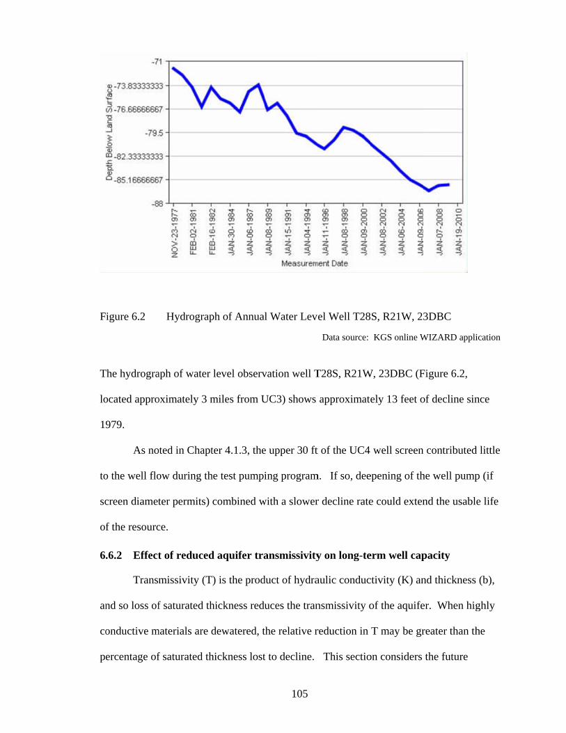
F
T
lo
19
to
sc
of
6
an
co
pe
igure 6.2
The hydrogra
ocated appro
979.
As no
o the well flo
creen diamet
f the resourc
.6.2 Effect
Transm
nd so loss of
onductive m
ercentage of
Hydrograp
aph of water
oximately 3 m
ted in Chapt
ow during th
ter permits)
ce.
t of reduced
missivity (T
f saturated th
materials are d
f saturated th
ph of Annual
level observ
miles from U
ter 4.1.3, the
he test pumpi
combined w
d aquifer tra
T) is the prod
hickness redu
dewatered, t
hickness lost
105
l Water Lev
vation well T
UC3) shows
e upper 30 ft
ing program
with a slower
ansmissivity
duct of hydra
uces the tran
the relative r
t to decline.
el Well T28
Data source:
T28S, R21W
approximate
t of the UC4
m. If so, dee
r decline rate
y on long-te
aulic conduc
nsmissivity o
reduction in
This sectio
S, R21W, 23
KGS online W
W, 23DBC (F
ely 13 feet o
well screen
epening of th
e could exten
erm well cap
ctivity (K) an
of the aquife
T may be gr
on considers
3DBC
WIZARD appli
Figure 6.2,
of decline sin
contributed
he well pump
nd the usable
pacity
nd thickness
er. When hig
reater than th
the future
ication
nce
d little
p (if
e life
(b),
ghly
he

106
production potential of wells completed in the Ogallala by factoring in the effects of
changed drawdown behavior as a consequence of reduced transmissivity.
In the Hecox et al. (2002) paper, KGS estimated the minimum saturated thickness
required to sustain 90 days of flow to production wells, choosing 50 gpm, 400 gpm and
1,000 as the example production rates. The analysis modeled both single wells and well
arrays on quarter-section centers (minimum well spacing approximately 2,600 ft) and was
based on available estimates of Ogallala hydraulic conductivity (K) and thickness. For
higher K (200 ft/day) portions of the aquifer, Hecox et al. (2002) estimated that at least
60 ft of saturated thickness was required to sustain multiple wells at 1,000 gpm and 40 ft
needed for 400 gpm. For lower K (25 ft/day) portions of the aquifer, KGS estimated 150
ft of ST is required to sustain 1,000 gpm and 90 ft is required for 400 gpm.
The reported UC3 transmissivity value in 1979 (Dealy and Jenkins 1980) was
160,000 gpd/ft and based on the reported aquifer thickness of 43 ft, this indicates a
hydraulic conductivity of 520 ft/day, which is considered a high K value. The reported
UC4 T value in 1977 (Burns and McDonnell 1977), as indicated by the response of both
the pumping well and nearby observation wells, was approximately 45,000 gpd/ft. If we
take the aquifer thickness in 1977 to be the difference between the base of the producing
zone determined in the spinner survey and the static water level, then the Ogallala
saturated thickness was about 300 ft, indicating a low to moderate K value of 20 ft/day at
that well location. Based on Hecox et al. (2002), at least 150 ft of ST would be required
to sustain 1,000 gpm for 90 days at UC4, and at UC3, the ST requirement could be as low
as 30 ft (KGS did not assess K values higher than 200 ft/day).
Subtracting the approximate relative declines at both wells sites of 15 ft for UC3
and 100 ft for UC4, and assuming an equivalent bulk K value for the remaining saturated

107
aquifer at both locations, the year 2010 effective transmissivity is estimated to be 109,000
gpd/ft at UC3 and 30,000 gpd/ft at UC4. Thus at both sites, approximately 30% of the
late 1970s transmissivity has been lost due to the effects of depletion. To depict this
change, a predictive drawdown spreadsheet developed by the Halford and Kuniansky
(2002) was used to check the validity of these estimates by simulating a 24 hour
drawdown test as shown in Figures 6.3 through 6.6. This spreadsheet is referred to as the
confined prediction worksheet, and is based upon the Theis equation. Although the
Ogallala is geologically an unconfined (water-table) system throughout much of western
Kansas, the pumping test response observed in wells UC3 and UC4 indicated the aquifer
behaves like a confined system especially for longer pumping durations.
For each well, the first confined prediction plot shows the “base case” defined as
the year the original pumping tests occurred in the late 1970s. The second plot shows the
predicted drawdown curve in 2010 based upon the reduced aquifer thickness and
transmissivity. The K values used in the base case prediction were adjusted slightly from
the values depicted above in order to obtain a good match between the base-case
predicted and actual drawdown. These calibrated values were 520 ft/day for UC3 and 18
ft/day for UC4. The 1977 transmissive thickness was also adjusted at UC4 from 300 to
250 ft. Only the base case and year 2010 conditions are illustrated, but given any
projected groundwater decline rate, future years could be modeled using this technique.

108
Figure 6.3 Base case (1979) predicted drawdown curve for UC3
Well UC3 1979 Case Drawdown Prediction for Confined Aquifers, Theis(1935)
Input Data for prediction of drawdown
Hydraulic conductivity, K, ft/day 520Aquifer Thickness, b, ft 43Storage Coefficient, S 0.005Pumping Rate, GPM 670Distance from well, ft 0.1
0
2
4
6
8
10
12
0:00:01 0:00:09 0:01:26 0:14:24 2:24:00 24:00:00
DR
AW
DO
WN
IN
FE
ET
TIME IN HOUR:MINUTE:SECOND
PREDICTED DRAWDOWN SEMI LOG
Equation used in prediction
s is drawdown, W(u) is the well function
T
uWQs
4
))((
Tt
Sru
4
2
0
2
4
6
8
10
12
0:00:00 3:00:00 6:00:00 9:00:00 12:00:00 15:00:00 18:00:00 21:00:00 24:00:00
DR
AW
DO
WN
IN F
EE
T
TIME IN HOUR:MINUTE:SECOND
PREDICTED DRAWDOWN LINEAR PLOT
0.01 0.1 1 10 100 1000
K
0.000001 0.00001 0.0001 0.001 0.01 0.1 1
S

109
Figure 6.4 Year 2010 predicted drawdown response for UC3
Well UC3 2010 Case Drawdown Prediction for Confined Aquifers, Theis(1935)1979 24 hour drawdown = 9.6 ftInput Data for prediction of drawdown
Hydraulic conductivity, K, ft/day 520Aquifer Thickness, b, ft 27Storage Coefficient, S 0.005Pumping Rate, GPM 670Distance from well, ft 0.1
0
2
4
6
8
10
12
14
16
0:00:01 0:00:09 0:01:26 0:14:24 2:24:00 24:00:00
DR
AW
DO
WN
IN
FE
ET
TIME IN HOUR:MINUTE:SECOND
PREDICTED DRAWDOWN
Equation used in prediction
s is drawdown, W(u) is the well function
T
uWQs
4
))((
Tt
Sru
4
2
0
2
4
6
8
10
12
14
16
0:00:00 3:00:00 6:00:00 9:00:00 12:00:00 15:00:00 18:00:00 21:00:00 24:00:00
DR
AW
DO
WN
IN F
EE
T
TIME IN HOUR:MINUTE:SECOND
0.01 0.1 1 10 100 1000
K
0.000001 0.00001 0.0001 0.001 0.01 0.1 1
S
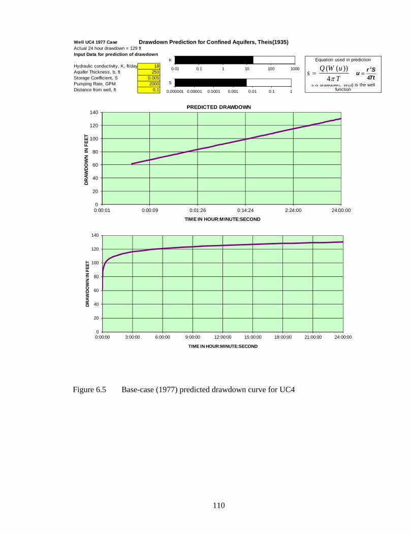
110
Figure 6.5 Base-case (1977) predicted drawdown curve for UC4
Well UC4 1977 Case Drawdown Prediction for Confined Aquifers, Theis(1935)Actual 24 hour drawdown = 129 ftInput Data for prediction of drawdown
Hydraulic conductivity, K, ft/day 18Aquifer Thickness, b, ft 250Storage Coefficient, S 0.005Pumping Rate, GPM 2000Distance from well, ft 0.1
0
20
40
60
80
100
120
140
0:00:01 0:00:09 0:01:26 0:14:24 2:24:00 24:00:00
DR
AW
DO
WN
IN
FE
ET
TIME IN HOUR:MINUTE:SECOND
PREDICTED DRAWDOWN
Equation used in prediction
s is drawdown, W(u) is the well function
T
uWQs
4
))((
Tt
Sru
4
2
0
20
40
60
80
100
120
140
0:00:00 3:00:00 6:00:00 9:00:00 12:00:00 15:00:00 18:00:00 21:00:00 24:00:00
DR
AW
DO
WN
IN F
EE
T
TIME IN HOUR:MINUTE:SECOND
0.01 0.1 1 10 100 1000
K
0.000001 0.00001 0.0001 0.001 0.01 0.1 1
S

111
Figure 6.6 Year 2010 predicted drawdown curve for UC4
The implication of reduced transmissivity is that if for example UC4 was test
pumped in 2010 at a constant rate of 2,000 gpm, the S value (change in drawdown per
log cycle of time) would be greater than the adjusted base case 1977 value of 18 ft, due to
a lower transmissivity, which in turn would reduce the calculated Q100d or Q20 value.
Well UC4 2010 Case Drawdown Prediction for Confined Aquifers, Theis(1935)1977 24 hour drawdown = 129 ftInput Data for prediction of drawdown
Hydraulic conductivity, K, ft/day 18Aquifer Thickness, b, ft 160Storage Coefficient, S 0.005Pumping Rate, GPM 2000Distance from well, ft 0.1
0
50
100
150
200
250
0:00:01 0:00:09 0:01:26 0:14:24 2:24:00 24:00:00
DR
AW
DO
WN
IN
FE
ET
TIME IN HOUR:MINUTE:SECOND
PREDICTED DRAWDOWN
Equation used in prediction
s is drawdown, W(u) is the well function
T
uWQs
4
))((
Tt
Sru
4
2
0
50
100
150
200
250
0:00:00 3:00:00 6:00:00 9:00:00 12:00:00 15:00:00 18:00:00 21:00:00 24:00:00
DR
AW
DO
WN
IN F
EE
T
TIME IN HOUR:MINUTE:SECOND
0.01 0.1 1 10 100 1000
K
0.000001 0.00001 0.0001 0.001 0.01 0.1 1
S
112
Examining either Figure 6.4 or 6.6, or re-arranging either the Theis (1935) or the Cooper-
Jacob (1946) equations makes it possible to estimate the change in drawdown behavior.
For UC4, using Cooper-Jacob, the estimated 2010 S at 2,000 gpm would be
approximately 25 ft per log cycle of time. This is significantly higher than the observed
1977 value of 11.7 ft or the confined prediction modeled value of 18 ft. If this 25 ft S
value is used in the Method B Moell Q20 calculation spreadsheet (without changing the
100 minute drawdown value), then the estimated Q20 value would be approximately 288
gpm, compared to the 983 gpm value calculated for 1977 test conditions, a 70% decrease,
and 398 gpm calculated in Chapter 6.6.1 solely on the basis of reduced available
drawdown. Due to lower T, the actual 100 minute drawdown would be higher in 2010,
and so the 288 gpm value might be optimistic. If the 25 ft S value is used in the Method
C Q100d calculation spreadsheet, then the 2010 Q100d value would be 277 gpm compared
to 1,165 gpm under 1977 test conditions (a 75% decrease).
Again using Cooper-Jacob, the estimated S for UC3 at 670 gpm would be 1.6
feet, as compared to the observed 1979 value of 1.2 ft. Using the 1.6 ft value in the Moell
worksheet results in a Q20 of 550 gpm compared to the 905 gpm value calculated for
1979 test conditions, a 40% decrease.
If we assume approximately 80 ft of ST remained at UC4 in 2010, then the Hecox
et al. (2002) estimate of 400 gpm (for K value of 25 ft/day) compares favorably with the
above estimates of 288 to 398 gpm. It is more difficult to draw comparisons for UC3,
because of the apparent high hydraulic conductivity of the Ogallala at the well location.
The 550 gpm Q20 value, and the high K suggest that even with a ST as low as 25 ft,
moderate well production in the range of 400 to 600 gpm might be feasible, but would
require a pumping test to confirm.

113
In summary, even though UC3 and UC4 are located considerable distance apart
and the thickness and hydraulic properties of the Ogallala aquifer are quite different at
each location, the groundwater decline that has occurred since the late 1970s has
effectively reduced aquifer transmissivity by about 25 to 30% at both well sites. This
change results in a corresponding decrease in theoretical long-term well capacity ranging
from 40% (UC3) to as much as 75% (UC4). The effect has been more pronounced in
Finney County (UC4) due to the fact that large declines have occurred, and the aquifer
exhibits a relatively low hydraulic conductivity.
Even if the Ogallala decline rate moderates near UC3 and UC4 and other similar
localities over the next 20 years, by 2030 a further decrease in the theoretical and actual
well capacity is likely. From this, it is clear that the magnitude of the declines seen in
parts of western Kansas, should they continue even at a slower rate through a planned
depletion policy (Sophocleous 2009), could be expected to significantly limit the ability
of individual wells to operate at their historically used flow rates.
6.7 USE OF ANALYTICAL AND NUMERICAL MODELS
Analytical models may be used to simulate groundwater pumping from one or
more wells, based on the Theis equation or other pumping test analytical methods; other
analytical tools can simulate groundwater flow in two-dimensions and thus can generate
drawdown contours. Numerous spreadsheet tools exist to generate a prediction of
drawdown at varying distances from a pumping well, including the USGS “Confined
Prediction” spreadsheet discussed in Chapter 6.6 (Halford and Kuniansky 2002), which
uses the following formula (based on the Theis equation) to generate values for
drawdown (s):

C
ex
sc
co
el
di
si
ec
sc
co
pu
hy
m
or
Commercial s
xpressions to
cenarios spe
ould incorpo
lement type
imensional t
ignificant ex
cological or
cenarios that
onceptual hy
umping tests
ydraulic pro
models now h
rder to gener
software too
o generate si
cified by the
orate several
and finite-di
transient cap
xchanges bet
water user c
t cannot be a
ydrogeologic
s, combined
perties is req
have the cap
rate both aqu
ols used in aq
imulated dra
e use; these s
analytical a
ifference typ
pabilities. Wh
tween surfac
conflicts, the
addressed thr
c modeling.
with detaile
quired in ord
ability to inc
uifer and pum
114
quifer test an
awdowns in
simulations a
aquifer test m
pe are more s
hen relativel
ce water and
en a flow mo
rough conve
Detailed as
ed informatio
der to constr
corporate we
mping well
nalysis apply
one or multi
are not limit
models. Num
sophisticated
ly large pum
groundwate
odel is a tool
entional pum
sessment of
on on hydros
ruct numeric
ell hydraulic
drawdown v
y similar ma
iple wells, b
ted to a Thei
merical mod
d tools that h
mping rates o
er are expect
l of choice to
mping test an
f well capacit
stratigraphy
cal models.
cs (e.g. well
values.
thematical
ased on pum
is analysis bu
els, both fin
have three-
occur, and
ted, with pos
o examine
nalysis and
ties based up
and aquifer
Numerical
efficiency) i
mping
ut
ite-
ssible
pon
in
115
CHAPTER 7
CONCLUSIONS
Of the various methods known to be applied in North America to estimate the
long-term capacity of individual wells, three were investigated in detail and applied in
quantitative analysis using eleven pumping test data sets. These are the methods of
Farvolden (1959), Moell (1975) and B.C. Ministry of Environment (CPCN; 1999) herein
referred to as Methods A, B and C.
This Chapter reviews the principal findings of the investigation and identifies
opportunities for further research. In summary, the objective of compiling pumping test
data sets from wells completed in a variety of hydrogeologic settings was successfully
applied to test three methods used to estimate long-term well capacity. The results were
interpreted along with conventional pumping test data analysis and other factors of
relevance to groundwater resource management. Research findings including
confirmation of the hypothesis, and the broader implications of the investigation are
presented below.
7.1 FINDINGS ON THE Q20 METHODS A AND B OF FARVOLDEN AND MOELL
This study confirms the finding of Maathuis and van der Kamp (2006) that the
Farvolden method may not be a reliable indicator of LTWC. Depending on the well test
conditions, Farvolden may in fact significantly over-estimate or under-estimate well
capacity. This is due to the fact that the early time drawdown value (in the first minute of
pumping) is not taken into account in the equation. This study devised an easy way to
test of the validity of the result by calculating specific capacity Ratio 1, a value which
should always be less than 1.0.
116
Interestingly, the Farvolden method did not tend to over-predict Q20 in lower-yielding
wells with large available drawdowns, represented in this study by the three fractured
bedrock aquifer wells. It is believed that this is because in such wells, the early time
drawdown is dominated by casing storage effects and as pumping continues, the rate of
drawdown usually increases.
The Moell method or the modified Moell method as proposed by Maathuis and
van der Kamp (2006) appears to produce reasonable Q20 values with specific capacity
ratios that support the validity of the results.
Both the Farvolden and the Moell methods are fairly sensitive to adjustments in
the default safety factor of 0.7. The sensitivity analysis showed that it is not likely
necessary to alter this factor by any more than 0.1 in specific situations. For pumping
tests that are long enough to determine the appropriate analytical conceptual model but
not long enough to ascertain the long-term drawdown pattern, detailed analysis as
suggested by Maathuis and van der Kamp (2006) may be warranted.
The temporal sensitivity to a LTWC value, as calculated by the Q20 methods to
other assumed pumping durations, such as 2 years or 200 years, is directly related to the
aquifer transmissivity and the drawdown behaviour as represented by the specific
capacity ratio. Since it is easy to calculate a Q2 and a Q200 value and a Ratio 1 or 2 from
any Q20 pumping test analysis, this is likely to prove insightful in many cases.
The sensitivity analysis also showed that the effect of increasing or decreasing
pumping time by an order of magnitude, in most cases, had a similar effect on the
resulting Q20 value as changing the safety factor by 0.1 (usually about 15%), except for
wells with a high Ratio 1 or 2 value, which tend to have Q20 values that are more
sensitive to changes in the safety factor.
117
7.2 FINDINGS ON THE Q100d METHOD C (CPCN)
The CPCN method appears to be a reliable tool in examining long-term well
capacity. Other than the pumping time, the main difference between this method and the
Q20 methods is the assumption that recharge occurs annually, and that the late-time
drawdown trend (if it plots on a straight line on a semi-log graph) should be used to
predict the 100-day drawdown value. The Q20 methods do not specify which portion of a
pumping test drawdown curve should be used. When the conceptual hydrogeologic
model is consistent with the observed drawdown behaviour, for example, well UC2
which exhibited the effects of a probable linear no-flow boundary during the pumping
test, then it is appropriate to use the late time drawdown trend. In the case of UC2, this
resulted in a more conservative Q100d and Q20 estimate.
The Q100d is a more practical method to assess long-term well capacity for wells
that are not likely to be pumped on a near continuous basis for more than a few months,
such as irrigation wells, or other water supply wells used seasonally.
Like the Q20 methods, the CPCN method shows fairly consistent sensitivity to
order of magnitude changes in pumping time or a 0.1 adjustment in safety factor and as
with the Q20 methods, the CPCN method appears to show roughly the same sensitivity to
a one order of magnitude change in pumping time as a 0.1 change in the safety factor.
7.3 IMPLICATIONS FOR GROUNDWATER MANAGEMENT
The hypothesis that the three promising but under-utilized methods for estimating
LTWC are viable for broader application was confirmed by the results of the study. The
comparative analysis showed the relative strengths and weaknesses of the three methods,
and the sensitivity of the methods to changes in variables, thus supporting the second part
of the hypothesis. The following sections summarize the key relationships between

118
individual well capacity and implications for aquifer capacity studies and groundwater
management.
7.3.1 Municipal and other semi-continuously used wells
For municipal wells, which typically operate year-round if they are primary water
sources for a water system, it is advisable to consider the future-projected Q20 value
determined with Method B or a modified Method B, for the water supply must be
available year-round (even if water demand is higher in summer). If 20 years is too long
of a time horizon for planning, the pumping time may be easily adjusted either by an
order of magnitude to 2 years or some intermediate value that may be determined
mathematically or by plotting Q2, Q20 and Q200 on a graph and interpolating. For well
fields and situations where groundwater use is intensive there may be issues of well
interference and/or streamflow capture to consider. Further assessment beyond the
capability of a long-term well capacity analysis is indicated for such cases, which may
involve increased monitoring of groundwater and surface water, pumping tests, detailed
water budget analysis, and groundwater flow modeling.
7.3.2 Irrigation and other seasonally used wells
The irrigation season varies according to climate and weather patterns and the
crops being irrigated, but is typically part of a year. For irrigation wells or any seasonally
used groundwater source, a Q100d value may be more applicable for determining the
annual long-term well capacity; but this value must be updated and corrected if the
situation changes, such as increased well development or groundwater level decline.
Well interference may be accounted for in most situations by reducing the HA
value by the amount of interference expected. If well interference represents a significant
percentage of saturated thickness in an unconfined aquifer, further analysis on the effect
119
of reduced transmissivity may be warranted. Any further uncertainties may be addressed
by either reducing the safety factor by 0.1 or extending the pumping time by one order of
magnitude.
7.3.3 Wells in groundwater decline situations based on the Ogallala case
The current and future yield of Kansas High Plains (Ogallala) aquifer wells (or
any well located in an area with documented groundwater decline) may be reasonably
well-predicted using either the Q100d or Q20 methods, provided that sufficient data exist to
constrain the bulk K value of the aquifer, which would ideally be from a previous or
recent pumping test, and a record of groundwater levels is available for the area of
interest. The drawdown behavior under current and future conditions can be predicted
using relatively simple techniques such as the USGS confined prediction spreadsheet tool
illustrated in Chapter 6.6.
The irrigation season in western Kansas typically ranges from 90 to 110 days for
crops such as sunflower, corn, grain sorghum and soybeans (Lamm et al. 2006).
Therefore, for Ogallala irrigation wells, a Q100d value is considered applicable for
determining the annual long-term well capacity; but this value must be updated and
corrected frequently if there is a continuing decline or if the pattern of decline changes.
Recall that a key assumption in the Method C (CPCN) is that recharge occurs after 100
days, which is not the case with the over-subscribed Ogallala system.
Municipal wells that have never been subjected to a controlled pumping test
should be tested if information on the long-term water supply is needed for planning
purposes. If done, this testing should be combined with a downhole flowmeter (spinner)
survey so that the actual production through the well screen or open interval may be

120
measured and compared to lithologic logs, thus enabling an integration of the PST
method of Macfarlane et al. (2005) with site-specific well data.
As the Ogallala system continues to lose saturated thickness, sustaining or
increasing municipal pumping rates could require ever larger areas of the aquifer to be
reserved for municipal production and other high priority groundwater uses, because the
net output per well might decrease as saturated thickness and transmissivity values fall.
The implication here is that in future more municipal wells may be needed not only to
sustain population growth in urban or town centers, but also because the average yield per
well will likely be lower than historic pumping rates.
7.4 OPPORTUNITIES FOR FURTHER RESEARCH
As Allen (1999) noted, coming up with an appropriate standard for the length of a
pumping test is challenging. On the one hand, pumping tests are relatively costly and
time-consuming procedures, and so there is a tendency in water management to rely on
modeling using averaged or assumed aquifer hydraulic properties. On the other hand, as
Butler (2009) noted, pumping tests are practically indispensable when the task is to assess
well and aquifer hydraulic properties and assess groundwater supplies. Some of the well
test data sets used in this analysis exhibited boundary effects during the test that had they
gone undetected, could have led to either an over-estimation or an underestimation in
LTWC. The two Ogallala aquifer wells assessed in this research underscore the highly
variable nature of this aquifer system and how differently the effects of depletion might
impact well production.
The author is aware of well tests that have encountered significant boundary
conditions occurring ten days or more into a constant rate aquifer test. Much has been
written on pumping test procedures, such as how to control and measure the flow rate,
121
how often to record water levels, the use of observation wells, and so on, but relatively
little consensus has emerged from the literature on pumping test duration, especially as it
relates to the task of determining well capacity as opposed to estimating aquifer
properties. Further research into the applicability and utility of longer-term pumping tests
could provide insight into the relative value on the information provided by the data,
versus what could be derived from extrapolation, assumptions, and modeling.
Another area for further research would be to expand the analysis presented here
to include a broader spectrum of well and aquifer types, and development of a tool that
could be used to rapidly estimate long-term well capacity and specific capacity ratios as a
routine exercise in the analysis of any pumping test. Just as the calculation of
transmissivity, storativity and specific capacity are part of the routine analysis of water
well pumping tests, the same could be done to examine LTWC under both test conditions
and assumed future conditions that may incorporate well interference, water level decline,
or a decrease in well performance (specific capacity). Broader application of the LTWC
methodologies has the potential to better inform water management decisions and is
therefore recommended as a supplement and not as a replacement for existing
methodologies such as modeling or water budget analysis. Within Kansas, the
opportunity exists to re-assess historical pumping test data reportedly on file for
numerous Ogallala wells as described in Table 3 of Hecox et al. (2002).
It is relatively easy to estimate LTWC values for virtually any well subjected to a
pumping test. It is not known why quantitative methods to estimate “safe well yield”
(LTWC) are not more widely applied. Such an approach should only improve the
understanding that may be derived from traditional pumping test interpretation. Pumping
test data from the time of original well construction are potentially relevant to present-day
122
assessments of LTWC, provided that information on groundwater levels, well specific
capacity, pump performance, and other pertinent data are available.
The evaluation of individual well long-term capacities is recommended when a
water source is of particularly high value and there is a need to understand the long-term
operational characteristics whether or not there is detailed water balance information on
the aquifer system and its “safe” or “sustainable” yield. A Q20 analysis is probably best-
suited to municipal wells or other sources used year-round on a perennial basis, while a
Q100d analysis may be better suited to irrigation wells or other wells used only seasonally
(for example, wells used at resorts).
Further spreadsheet or software tools could be developed to enable prediction of
Q20 or Q100d using any analytical model, as recommended by Maathuis and van der Kamp
(2006). Some of these models involve matching the observed data to one of a family of
related drawdown curves. In the case of predicting long-term well capacity, the proper
match must include a good-fit for the later time drawdown trend as this trend would
likely need to be used in the Q20 or Q100d calculation.

123
REFERENCES
Alberta Environment, 2003. Groundwater Evaluation Guideline (information required when submitting an Application under the Water Act).
Allen, D., 1999, An assessment of the methodologies used for analyzing hydraulic test data from bedrock wells in British Columbia: Earth Science Department of Simon Fraser University and prepared for the British Columbia Ministry of Environment, Lands and Parks Groundwater Section.
Allen, D., A. Badry, B. Ingimundson, G. Wendling, B. Worobets and N. Morrison, 1999, Evaluating long-term capacity for a Certificate of Public Convenience and Necessity: Report for Water Management Branch, B.C. Ministry of Environment, Lands, and Parks, Victoria.
Alley, W.M., T.E. Reilly, O.L. Franke, 1999, Sustainability of ground water resources: U.S. Geological Survey Water Supply Circular 1186, 79 p.
Alley, W.M. and S.A. Leaky, 2004, The journey from safe yield to sustainability: Ground Water v. 42, No. 1. p 12-16.
Anderson, M. and W. Woessner, 1992, Applied groundwater modeling: Academy Press, San Diego, Calif., 381 p. AqtesolvTM, 2010. Software program for analyzing pumping tests, slug tests and constant head tests: HydroSolve, Inc. Archfield, S., R. Vogel, P. Steeves, S. Brandt, P. Weiskel, and S. Garabedian, 2009, The Massachusetts sustainable yield estimator: A decision support tool to assess water availability at ungauged stream locations in Massachusetts: Scientific Investigations Report 2009-5227. U.S. Department of Interior, U.S. Geological Survey, 129 p. Baker, D. 1955, Safe yield of ground-water reservoirs: Assemblee Generale de Bruxelles, Assoc. International Hydrologie Scientifique, v. 2, p. 160-164.
B.C. Ministry of Environment, 1999, Evaluating long-term well capacity for a Certificate of Public Convenience and Necessity: ISBN 0-7726-4019-X.
Bibby, R., 1979, Estimating sustainable yield to a well in heterogeneous strata: Alberta Research Council Bulletin No. 37.
124
Bourdet, D., J. Ayoub, and Y. Pirard, 1989, Use of pressure derivative in well test interpretation: SPE publication 19215, p. 293-302.
Bredehoeft, J., S. Papadopulos, and H. Cooper, 1982, Groundwater - the water-budget myth: in Scientific basis of water-resource management: National Academy Press, p. 51-57.
Bredehoeft, J., 1997, Safe yield and the water budget myth: Ground Water v. 35, No. 6: p. 929. Bredehoeft, J. and T. Durbin, 2009, Groundwater development – the time to full capture problem: Ground Water v. 47 No. 4, p. 506-514.
Burns and McDonnell,1977, Report on the groundwater resources investigation of the Spratt site for the proposed coal-fired generating plant, Holcomb, Kansas: Report prepared for Sunflower Electric Cooperative, Inc. (excerpts of well test data and well logs).
Butler, J.J., 2009, Technical commentary: Pumping tests for aquifer evaluation – time for a change?: Ground Water, v.5, No. 5, p. 615-617. Cobb, P.M., C.D. McElwee and M.A. Butt, 1982, Analysis of leaky aquifer pumping test data: An automated numerical solution using sensitivity analysis: Ground Water v. 20, No. 3 p. 325-333.
Cooper, H. and C. Jacob, 1946, A generalized graphical method for evaluating formation constants and summarizing well field history: Transactions of American Geophysical Union, 27, p. 526-534.
Dealy, M.T. and E.D. Jenkins, 1980, Groundwater resources of southeast Ford County, Kansas: Southwest Kansas Groundwater Management District #3, Garden City, 47 p.
Devlin J. and M. Sophocleous, 2005, The persistence of the water budget myth and its relationship to sustainability: Hydrogeology Journal, v. 13. p. 549-554.
Driscoll, F., 1986, Groundwater and wells. 2nd Ed., St Paul, Johnson Division, 1089 p.

125
Farvolden, R., 1959, Groundwater supply in Alberta: Unpublished Alberta Research Council report. (provided in an appendix to Maathuis and van der Kamp 2006).
Ferris, J., D. Knowles, R. Brown and R. Stallman, 1962, Theory of aquifer tests: U.S. Geological Survey Water Supply Paper 1536-E, 174 p.
Fetter, C., 2001, Applied Hydrogeology, 4th Ed. Upper Saddle River, Prentice Hall, 598 p.
Gingarten, A.C. and P.A. Witherspoon, 1972, A method of analyzing pumping test data from fractured aquifers: Journal International Association of Rock Mechanics.
Groundwater Management District 3, 2004, Revised Water Management Program: Southwest Kansas Groundwater Management District No. 3. Halford, K.J. and E.L. Kuniansky, 2002, Documentation of spreadsheets for the analysis of aquifer test and slug test data: U.S.Geological Survey Open-File Report 02-197. Harbaugh, A.W., E.R. Banta, M.C. Hill and M.G. McDonald, 2000, MODFLOW 2000, the U.S. Geological Survey modular ground-water flow model: User guide to modularization, concepts and the groundwater flow process: U.S. Geological Survey Open-File Report 00-92. Hecox, G.R., P.A. Macfarlane, and B.B. Wilson, 2002, Calculation of yield for High Plains wells: relationship between saturated thickness and well yield: Kansas Geological Survey Open-File Report 2002-25C. Jacob, C., 1946, Drawdown test to determine effective radius of artesian wells: Transactions of American Society of Civil Engineers, v. 112, p. 1047-1070. Jacob C. and S. Lohman, 1952, Non-steady flow to a well of constant drawdown in an extensive aquifer: Transactions of American Geophysical Union v. 33, p. 559-569.
Kalf, R. and D. Woolley, 2005, Applicability and methodology of determining sustainable yield in groundwater systems: Hydrogeology Journal, v. 13, p. 295-312.
Kansas Geological Survey, 2010, Online water level (Wizard) and well record search (WWC5) for Ford and Finney Counties, Kansas in Groundwater Management District #3.
126
Kendy, E. ,2003, The false promise of sustainable pumping rates: technical commentary. Ground Water, v. 41, No. 1, p 2-4.
Konikow, L.F., 2010, Representing pump-capacity relations in groundwater simulation models: Ground Water, v. 48. No. 1, p. 106-110.
Kruseman G.P. and N.A. de Ridder, 1990, Analysis and evaluation of pumping test data, 2nd Ed., Wageningen, NL: International Institute for Land Reclamation and Improvement, 377 p.
Lamm, F.R., L.R. Stone and D.M. O’Brien, 2006, Crop production in western Kansas as related to irrigation capacity: in Proceedings of the 2006 ASABE Annual International Meeting, Portland, Oregon. Contribution No. 06-319-A.
Lee, C., 1915, The determination of safe yield of underground reservoirs of the closed basin type: Transactions of American Society of Civil Engineers, v. 78, p.148-151.
Lohman S.W. and others, 1968, Definitions of selected ground-water terms, revisions and conceptual refinements: U.S. Geological Survey Water-Supply Paper No. 1988, 78 p.
Lohman, S.W., 1982, Ground-water hydraulics: U.S. Geological Survey professional paper No. 708, 70 p.
Los Angeles County of Public Health, 2005, Well yield test procedures private wells.
Maathuis, H. and G. van der Kamp, 2006, The Q20 Concept: Sustainable Well Yield and Sustainable Aquifer Yield: Saskatchewan Research Council Publication No. 10417-4E06, 49 p., appendices. Macfarlane, P. A., B. Wilson and G. Bohling, 2005, Practical saturated thickness of the Ogallala in two small areas of Southwest Kansas Groundwater Management District 3: Kansas Geological Survey Open-File Report 2005-29. Macfarlane, P.A. and N. Schneider, 2007, Distribution of the permeable fraction and practical saturated thickness in the Ogallala portion of the High Plains Aquifer in southwest Kansas Groundwater Management District 3: Kansas Geological Survey Open-File Report 2007-28.
127
McCall, G.W., J.J Butler, Jr., J.M. Healey, A.A. Lanier, S.M. Sellwood, and E.J. Garnett, 2002, A dual-tube direct push method for vertical profiling of hydraulic conductivity in unconsolidated formations: Environmental and Engineering Geoscience, v. 8, No. 2, p. 75-84.
Meinzer, O.,1920, Quantitative methods of estimating groundwater supplies: Geological Society of America Bulletin, v. 31, p. 329-338.
Moell, C. , 1975, Guidelines – groundwater supply evaluations for residential subdivisions single-family wells: Alberta Environment Earth Sciences and Licensing Division: Report No. 1617. 8 p.
Neuman, S.P., 1975, Analysis of pumping-test data from anisotropic unconfined aquifers considered delayed gravity response: Water Resources Research, v. 12, p. 329-342.
Neville, C., 2008, Critical thinking in interpretation of pumping tests: Unpublished S.S. Papadopolous and Associates, short-course compilation.
Okanagan Basin Water Board, 2009, Okanagan Basin water supply and demand project report: Groundwater study objectives 2 and 3: Report prepared by Golder Associates Ltd. and Summit Environmental Consultants Ltd.
Ontario Ministry of Environment (OMOE), 2005a, Permit to take water manual: Ministry of Environment, Queen’s Printer for Ontario, PIBS 4932e.
Ontario Ministry of Environment (OMOE), 2005b, Guide to permit to take water application form: Ministry of Environment, Queen’s Printer for Ontario, PIBS 5046e.
Rivera, A., 2006, Current knowledge of the groundwater resources of Canada: in Proceedings of the joint USGS/CGS Meeting, Ottawa, Sept 14-15, 2006.
Rorabaugh,, J., 1953, Graphical and theoretical analysis of step-drawdown test of artesian well: Proceedings of American Society of Civil Engineers, v. 79, Separate 362.
Schulmeister, M.K., J.J. Butler, Jr., J.M. Healey, L. Zheng, D.A. Wysocki, and G.W. McCall, 2003, Direct-push electrical conductivity for high-resolution hydrostratigraphic characterization: Ground Water Monitoring and Remediation, v. 23, No. 3, p. 52-63.
128
Schulmeister, M.K., J.M. Healey, J.J. Butler, Jr., and G.W. McCall, 2004, Direct-push geochemical profiling: A new approach for assessment of inorganic chemical heterogeneity in aquifers: Journal of Contaminant Hydrology, v. 69, No. 3-4, p. 215-232. Schulmeister, M.K. and D.J. Geller, 2009, Progress Report: Scott City public water supply study (Contract 09-0127): Unpublished report submitted to Kansas Water Office.
Sophocleous, M., 1997, Managing water resource systems: why “safe”yield is not sustainable: Ground Water, v. 35, No. 4, p. 561.
Sophocleous, M., 1998, On the elusive concept of safe yield and the response of interconnected stream-aquifer systems to development: in Perspectives on Sustainable Development of Water Resources in Kansas: Kansas Geological Survey Bulletin 239, Lawrence, p. 61-85.
Sophocleous, M., 2000, From safe yield to sustainable development of water resources – the Kansas experience: Hydrogeology Journal, v. 235, p. 27-43.
Sophocleous, M., 2009, Review: Groundwater management practices, challenges and innovation in the High Plains aquifer, USA – lessons and recommended actions: Hydrogeology Journal, v. 18, p. 559-575.
Spane, F. and S. Wurstner, 1993, DERIV: A computer program for calculating pressure derivatives for use in hydraulic test analysis: Ground Water, v. 31 No. 5, p. 814-822.
Stallman, R.W., 1976, Aquifer test design, observation and data analysis: Techniques of Water-Resources Investigations of the U.S. Geological Survey: Book 3, Chapter B1.
State of Connecticut, 2009, Guidelines for determining yield of private wells: Publication No. 28.
State of Vermont, 2010, Agency of Natural Resources, Department of Environmental Conservation Environmental Protection Rules: Chapter 21, Water Supply Rule.
Theim, 1906, Hydrologische methoden (English translation:Hydrological methods). Leipsig: Gebhardt, 56 p.
129
Theis, C.V., 1935, The relation between the lowering of the piezometric surface and the rate and duration of discharge of a well using groundwater storage: Transactions of American Geophysical Union, v.16, p. 519-524.
Theis, C.V., 1940, The source of water derived from wells, essential factors controlling the response of an aquifer to development: Civil Engineering, v. 10, No. 5, p. 277-280.
Todd, D.K., 1959, Groundwater Hydrology: New York: J. Wiley & Sons, 336 p.
Toth, J., 1973, Hydrogeology and yield evaluation of a municipal well field, Alberta, Canada: Hydrological Science Journal. v. 8, No. 2 p. 165-189.
Township of Langley, B.C., 2010, Subdivision servicing bylaw, proof of water requirements.
Van der Kamp, G. and H. Maathuis, 2005, The applicability of Q20 methods for determining sustainable groundwater yields: in Proceedings of the 58th Canadian Geotechnical & 6th Joint IAH-CNC and CGS Conference, Saskatoon, SK, Canada.
Van der Kamp G. and H. Maathuis, 2006, Groundwater sustainability in the Prairies – some examples: in Proceedings of Sea to Sky Geotechnique Conference, p. 1288-1292.
Walton, W., 1970, Groundwater Resource Evaluation: New York, McGraw-Hill, 339 p.
Weight, W.D. and J.L. Sonderegger, 2001, Manual of Applied Field Hydrogeology. New York, McGraw-Hill, 608 p.
Williams, E.B., 1981, Fundamental concepts of well design: Ground Water, v. 19, No. 5, p. 527-542.


