Computers in Biology and Medicine 37 (2007) 83–96www.intl.elsevierhealth.com/journals/cobm

A multiresolution diffused expectation–maximization algorithm for medicalimage segmentation

Giuseppe Boccignonea,∗, Paolo Napoletanoa, Vittorio Caggianob, Mario Ferraroc

aNatural Computation Lab, DIIIE-Universitá di Salerno, via Ponte Don Melillo, 1, 84084 Fisciano (SA), ItalybDipartimento di Informatica e Sistemistica, Universitá di Napoli Federico II, via Claudio, 21, 80125 Napoli, Italy

cDipartimento di Fisica Sperimentale, Universitá di Torino, via P. Giuria, 1, 10100 Torino, Italy

Received 3 October 2005; accepted 3 October 2005

Abstract

In this paper a new method for segmenting medical images is presented, the multiresolution diffused expectation-maximization (MDEM)algorithm. The algorithm operates within a multiscale framework, thus taking advantage of the fact that objects/regions to be segmented usuallyreside at different scales. At each scale segmentation is carried out via the expectation–maximization algorithm, coupled with anisotropicdiffusion on classes, in order to account for the spatial dependencies among pixels. This new approach is validated via experiments on a varietyof medical images and its performance is compared with more standard methods.� 2005 Elsevier Ltd. All rights reserved.

Keywords: Image segmentation; Expectation–maximization; Multiresolution

1. Introduction

Computer algorithms for segmentation, the partitioning of animage into meaningful regions, play a crucial role in the delin-eation of anatomical structures of interest in several biomed-ical imaging applications, such as diagnosis, localization ofpathology, study of anatomical structures, treatment planningand computer integrated surgery. The process of image seg-mentation assigns pixels to regions defined by labels. For in-stance, in segmenting skin lesions, one label may be assignedto pixels within the lesion region, another label to pixels out-side such region; in magnetic-resonance (MR) images three la-bels may be used to distinguish gray-matter, white-matter andcerebrospinal-fluid tissue. Labeling is performed requiring cer-tain regularity constraints to be satisfied.

More formally, consider an image F defined on a domain �,then the segmentation problem is to determine the set of K re-gions Rk ⊂ �, k= 1, . . . , K , satisfying an homogeneity pred-icate H, such that: (1)

⋃Kk=1 Rk =�, with Rk ∩Rl �= ∅, k �=

l; (2) H(Rk) = true,∀k; (3) H(Rk ∪ Rl ) = false,∀Rk,Rl

∗ Corresponding author. Tel.: +39089964275; fax: +39089964218.E-mail addresses: boccig@unisa.it (G. Boccignone), pnapoletano@unisa.it

(P. Napoletano), vcaggian@unina.it (V. Caggiano), ferraro@ph.unito.it(M. Ferraro).

0010-4825/$ - see front matter � 2005 Elsevier Ltd. All rights reserved.doi:10.1016/j.compbiomed.2005.10.002

adjacent. The first condition states that the partition has to coverthe whole image and that any given pixel cannot belong to tworegions; the second indicates that each region has to be uniformwith respect to the predicate H; the last condition prevents twoadjacent regions from being merged into a single region thatsatisfies H.

A wide array of techniques, both for gray-level and colorimages, has been used in the past (for in-depth surveys, see[1–3]) either exploiting image-domain or feature-space basedapproaches but so far there is no satisfactory solution to imagesegmentation.

Image-domain based techniques try to account for feature-space homogeneity while ensuring spatial compactness, forinstance by progressively growing image regions or either bysubdividing and merging the regions according to a feature-based predicate H (e.g, color similarity) [4]. Classical regiongrowing, however, is not completely automated, since initialseed points must be given from which regions are grown. Split-and-merge techniques do not require seed points [5], but theymay exhibit over-segmentation, with the occurrence of manysmall, disconnected regions; in order to promote significantregions, multiresolution schemes can be applied. Multiresolu-tion provides an interesting strategy to carry out the refinementof segmentation [6,7], by operating on the image at different

84 G. Boccignone et al. / Computers in Biology and Medicine 37 (2007) 83–96

scales/resolutions, using for instance a quadtree, wavelets [7]or a pyramid structure [8]. Segmentation can also be obtainedby detecting edges among regions [1], however edges cannotbe used directly to define a region and further processing (edgelinking, grouping etc.) is then required. In general such classi-cal techniques have the critical limitation of using local criteria(pixel based). The homogeneity criterion has the function ofdeciding whether a pixel belongs to the growing region or notand the decision of merging is generally taken based only onthe contrast between the evaluated pixel and the region. How-ever, it is not easy to decide when this difference is small (orlarge) enough to take a decision. Limitations of purely localmethods has led to the use of Markov random fields (MRF)models (in particular Gibbs MRF), which combine local spa-tial interactions, also incorporating edge information, with aglobal cost function (e.g., energy) [9]. Difficulties associatedwith MRFs are the proper selection of the parameters control-ling the strength of spatial interactions, and that they requirecomputationally intensive algorithms [10]. Deformable models[11] (e.g., active contours), partial differential equations (e.g.,anisotropic diffusion [12]), and in general variational methodsrelying upon the minimization of some global energy func-tion, either related to image discontinuities (edges) or to regionuniformity, can be seen as deterministic counterparts of MRFs[13,14]. In general, active contours are sensitive to initial con-ditions and are really effective only when the initial positionof the contour in the image is sufficiently close to the realboundary.

Feature-space based techniques work out in some featurespace (e.g., color or texture) and solve the segmentation prob-lem by finding clusters (regions) in such space or by findingthe peaks of histograms (empirical distributions of the fea-tures); for instance, histogram thresholding is among the mostpopular technique [15]. The main limitations of this techniqueare that often, because of the noise, the profiles of the his-tograms are rather jagged giving rise to spurious peaks, andthat it does not take into account the spatial characteristics ofan image; furthermore the extension to color or multivaluedimages is not straightforward. Some of these problems can besolved by embedding connectivity information [16] or by re-sorting again to multiresolution representations, e.g., wavelets[17,18]. Clustering methods such as K-means, fuzzy c-meanscan be seen as unsupervised classifier methods [19], patternrecognition techniques that seek to partition (cluster) a fea-ture space derived from the image [1]. Of particular interestfor the work presented here, is that such clustering algorithmscan be given a generalized form [20] known in the literatureas the expectation–maximization (EM) algorithm, [21]. TheEM algorithm assumes that pixel intensities are independentsamples drawn from a linear combination of probability dis-tributions, usually Gaussians [22] (finite mixture model, seeSection 2 for details). In the E-step expectation–maximizationcomputes the posterior probabilities that a pixel belongs to acertain class, whereas in the M-step computes maximum like-lihood estimates of the parameters characterizing the distribu-tions (that for Gaussian distributions, correspond to means andcovariances), and mixing coefficients. Assignment to a class of

a pixel is eventually provided according to maximum poste-rior probability with respect to the given classes. Note that likethresholding and clustering algorithms, EM does not directlyincorporate spatial modeling and can therefore be sensitive tonoise and intensity inhomogeneities. To overcome such draw-backs several methods have tried to incorporate MRFs or, ingeneral, a prior term in order to maximize a log-posterior prob-ability instead of log-likelihood, thus leading to quite complexEM steps (see, for a discussion [23,24]). Recently, a diffusedexpectation–maximization (DEM) algorithm has been proposedfor gray-level images [25], in which a diffusion step providesspatial constraint satisfaction.

Here we presents a twofold extension of the diffusedexpectation–maximization approach: the algorithm will be ex-tended to deal with vector (i.e. color) images and furthermoreit will operate in a multiresolution framework to take advan-tage of the fact that objects/regions to be segmented usuallyreside at different scales.

2. Method

2.1. Theoretical background

Let the plane of the image be formed by N pixels, and letfi be the gray-level associated to the ith pixel; gray-levels aresupposed to be drawn from a finite set and range from 0 toM − 1, so that there are M possible values. More formally,any gray-level image can be considered a set of N unlabeledsamples F = {f1, f2, . . . , fN }, on a 2D discrete support � ⊆Z2, with N = |�|.

The image segmentation problem can be defined in prob-abilistic terms as the problem of assigning a label k to eachpixel i, given the observed data F, and where each label k ∈[1, . . . , K] defines a particular region/model. Different mod-els are selected with probability P(k), and a sample is gener-ated with probability distribution p(fi |k, �) where �={�k, k=1, . . . , K} and �k is the vector of the parameters associated tolabel k. Thus p(fi |k, �) is the probability of fi given the pa-rameters of all models and the fact that we have selected model(label) k. Each image can be conceived as drawn from a mix-ture density, so that, for any pixel,

p(fi |�)=K∑

k=1

P(k)p(fi |k, �); (1)

terms P(k) represent the mixing coefficients and it is usual toadopt the notation �k ≡ P(k). The likelihood of the data is

L= p(F |�)=N∏

i=1

p(fi |�). (2)

For clarity’s sake, we define two probability distributions p(fi)

and �(f ); the former is the probability that, given a gray-level fit is assigned to pixel i, so that

∑i p(fi)=1, whereas the latter

is the probability that, given any pixel i it has gray-level f. Thenp(fi) is a spatial distribution of the gray-levels across the im-age, whereas �(f ) is the probability to find a given gray-level f,

G. Boccignone et al. / Computers in Biology and Medicine 37 (2007) 83–96 85

irrespective of the position in the image. Image segmentationcan be achieved by finding the set of labels that maximizes thelikelihood L = ∏N

i=1∑K

k=1 P(k)p(fi |k, �), or, equivalently,by using Eqs. (1) and (2)

1

NlogL= 1

N

N∑i=1

logK∑

k=1

p(fi |k, �)P (k). (3)

By the weak law of large numbers and the ergodic theoremthe right-hand side of Eq. (3) can be written as the expectationwith respect to gray-level f

E

[log

K∑k=1

p(fi |k, �)P (k)

]

=M−1∑f=0

(�(f ) log

K∑k=1

p(fi |k, �)P (k)

). (4)

Simple manipulations lead to

1

NlogL=

M−1∑f=0

�(f ) log �(f )

−M−1∑f=0

(�(f ) log

�(f )∑Kk=1 p(fi |k, �)P (k)

). (5)

Hence a straightforward maximization of logL can beobtained by minimizing the second term of the last ex-pression, namely the Kullback–Leibler (KL) divergenceD(�(f )‖∑K

k=1 p(fi |k, �)P (k)) between distributions �(f )

and∑K

k=1 p(fi |k, �)P (k), while holding the first term fixed.This is exactly what is performed by the classic EM algorithm[21] which minimizes the KL divergence between the manifoldof the observed data and that of the true distribution.

In particular, when Gaussian distributions are used to modelthe density mixture of Eq. (1), the E- and M-steps can easilybe computed in closed form. Define hik = p(k|fi, �); in theE-step these posterior probabilities are given by

h(t)ik =

�(t)k p(fi |k, �(t)

k , �(t)k )∑

k �(t)k p(fi |k, �(t)

k , �(t)k )

(6)

while in the M-step, with h(t)ik fixed, the parameters � and mixing

proportions �k = P(k) that maximize logL, are obtained as

�(t+1)k = 1

N

∑i

h(t)ik , �(t+1)

k =∑

i h(t)ik fi∑

i h(t)ik

,

�(t+1)k =

∑i h

(t)ik [fi − �(t+1)

k ]2∑i h̃

(t)ik

, (7)

The E- and M-steps are iterated until | logL(t+1)−logL(t)|< �.Alternatively, one could attempt a multistep approach by iter-

atively minimizing the entropy H(f )=−∑M−1f=0 �(f ) log �(f ),

while holding p(F |k, �), P(k) fixed, and then minimizing thedivergence D, while keeping H(f ) fixed. Interestingly, from thesegmentation standpoint, the problem can be reformulated in

a way which takes into account the spatial correlations amongpixels, as follows.

Empirical approximations of probabilities p(fi) and �(f )

are given by

pi = p(fi) � fi

ftotand ftot =

N∑i=1

fi , (8)

and

�(f ) � nf

N, (9)

and the relation ftot=∑Ni=1 fi=∑M−1

f=0 nf f holds. From theseprobabilities two different entropies can be derived, namelyH and Hs, that capture different types of uncertainty related tothe stochastic process of which the image is a sample; from�(f ) the entropy H can be defined as

H(f )=−M−1∑f=0

�(f ) ln �(f ), (10)

whereas a spatial measure of entropy is

Hs =−N∑

i=1

p(fi) ln p(fi)= E

[ln

1

p(fi)

]. (11)

By making use of (8) and (9) it is not difficult to prove thatHs increases when H decreases. Intuitively, when the imageis uniform (all pixels have the same gray-level) Hs will bemaximum, while H will be 0 since there is only one gray-level f with probability p(f ) = 1. Thus a minimization ofH corresponds to a maximization of Hs.

The main idea behind the DEM approach is that maximiza-tion should be attained in a way label assignment to a pixel de-pends on the labels in the pixel neighborhood; then, a processmust be devised that takes into account spatial correlations. Ithas been proved [26] that−Hs=∑N

i=1 p(fi) log p(fi) is a Lia-punov functional decreasing under isotropic diffusion; howeverthis result as such does not allow to select the optimal label.Note that neighboring pixels should have the same probabilityto be assigned a given label k and that labels at boundaries be-tween regions should be characterized by an abrupt change ofprobability values. Thus, each hik = p(k|fi, �) field should bea piecewise constant function across the image and this resultcan be achieved [26] by a system of k anisotropic diffusionequations

�hik(t)

�t= ∇ · (g(∇hik)∇hik(t)) (12)

one for each label probability plane; g(·) is a suitable conduc-tance function, monotonically decreasing. Hence small differ-ences of hik among pixels close to each other are smoothedout, since diffusion is allowed, whereas large variations arepreserved. As in the isotropic case, anisotropic diffusion isproved to increase the spatial entropy Hs [26]. The DEMalgorithm obtains the maximization of logL by iteratively

86 G. Boccignone et al. / Computers in Biology and Medicine 37 (2007) 83–96

computing p(k|f, �), p(F |k, �), P(k) along the expectationand maximization steps via Eqs. (6), (7) and interleaving thiscomputation with diffusion on p(k|f, �), through Eq. (12)which in practice regularizes each k labeling field by propagat-ing anisotropically such labels. Eventually, the segmentationis performed by using the estimated parameters k, �k .

2.2. Extension to multi-valued images

A vector-valued (multi-valued) image can be considered a setof N unlabeled samples F= { f1, f2, . . . , fN }, on a 2D discretesupport � ⊆ Z2, with N = |�|, where each sample fi is aD-dimensional vector [f 1

i , f 2i , . . . , f D

i ]T; in other terms, F isa set of single-valued images {F 1, F 2, . . . , FD}, sharing thesame domain. A color image can be considered a vector-valuedimage, each component corresponding to one of the three colorchannels; for instance an RGB image, can be represented as{F R, F G, F B}.

A color space is a geometrical and mathematical representa-tion of color; there is a variety of such representations either de-rived from hardware considerations (e.g., RGB, YCrCb, NTSC,YIQ, CMYK, etc.), or colorimetry issues (e.g., XYZ, UCS,CIELAB, CIELUV), or visual perception motivations (Oppo-nent colors, IHS, HSV, etc.). A survey can be found in [27,28].We will use the YCrCb color space; this choice is motivated bythe fact that YCrCb de-correlates the original tristimulus colorcomponents, thus granting independence of the color channels.The mapping {F R, F G, F B} �→ {F Y, F Cr, F Cb} from the RGBspace to YCrCb space is accomplished through linear transfor-mation [28].

2.3. Multiresolution representation of images via pyramids

It has been observed previously that the DEM approach takesinto account the spatial interactions among pixels in the image;it should be noted, however, that different types of regions are,in general, characterized by different interactions lengths, e.g.points in almost uniform regions have longer interaction rangethan those in weak texture, and, moreover such range dependson the scale on which the analysis is performed [29]. Then theproblem arises on which is the optimal scale at which segmen-tation must be carried out: a low resolution might result in a toocoarse segmentation, with different regions merged together,whereas a high resolution, on the contrary could result in manyfragmented images and involves a heavy computational load.

In particular, when dealing with very complex images, suchas vector-valued images, clearly one should be concerned inobtaining reliable segmentation results, while keeping accept-able computational costs. Both issues can be accounted forby resorting to a multiresolution representation of the originalimage, e.g., a pyramidal representation [8]. On the one hand,propagation of information gained from coarse resolution lev-els makes significant objects/regions in the image more rele-vant respect to weak textures and noise. On the other hand,pyramids provide an efficient tool to reduce the computationalload both as regards the iterations necessary to maximize thelikelihood—by initializing the parameter set on the basis of the

parameters estimated at the coarser level—and for what con-cerns the diffusion step, which, at each iteration needs only towork upon a sub-sampled version the probability maps.

A multiresolution representation can be derived from theoriginal color image, by means of a Gaussian pyramid [8] ob-tained by performing a low-pass filtering via convolution with agaussian G(�l ) [8], l being the level of resolution, followed by asub-sampling of the smoothed scalar field, here the color chan-nel Fd , where the index d denotes the color component [30]:

fd,(l+1)i = S ↓ G(�l ) ∗ f

d,(l)i , (13)

where S ↓ is the down-sampling operator. Note that the transi-tion from scale l to scale l+1 produces a coarser representationof the image, and hence f

d,(0)i = f d

i , is the highest resolutionlevel and corresponds to the original image.

We will denote by P{Fd} the Gaussian pyramid build onthe scalar field, Fd , while P{F}={P{F 1}, . . . ,P{FD}}, is theGaussian pyramid representation of the vector-valued image.The level l of the pyramid P{F} will be indexed by P(l){F},or, for notational simplicity, by F(l).

Fig. 1 provides an example of the pyramidal decompositionof a computed tomography (CT) scan image rendered as a gray-level image. The pyramidal representation of a vector-valuedimage is shown in Fig. 2 by using a skin lesion image; inparticular, for visualization purposes, the “color” pyramid of thesame image is shown on the left (Fig. 2(a)), actually obtainedthrough the decomposition P{F}={P{F Y},P{F Cr},P{F Cb}}on the Y, Cr, Cb channels respectively, presented in the rightpicture Fig. 2(b).

In our implementation, pyramid depth is automatically com-puted given the size of the image at the coarsest level.

2.4. The MDEM algorithm

As previously remarked, a key property of pyramids isthat long range interactions can be captured by short pathsin the coarse levels, as the paths are through points repre-senting blocks of pixels instead of pixels. Such multireso-lution representation is used as follows. At a certain levell of the pyramid, different from the lowest resolution level,maximization of logL is obtained by iteratively computingp(k(l)|F(l), �(l)), p(F(l)|k(l), �(l)), P(k(l)) while diffusing onp(k(l)|F(l), �(l)) over sites i:

�p(k(l)| f(l)i , �(l))

�t

= ∇ · (g(∇p(k(l)f(l)i , �(l)))∇p(k(l)| f(l)i , �(l))); (14)

Eq. (14), defines a system of D diffusion equations for eachlabeling plane k.

As previously discussed, this step can be used to in-corporate spatial coherence into segmentation techniques.Using anisotropic diffusion on the posterior probabilitiesp(k(l)|F(l), �(l)) to capture local spatial constraints is moti-vated by the intuition that posteriors with piecewise uniformregions result in segmentations with piecewise uniform re-gions. Application of anisotropic smoothing on the posterior

G. Boccignone et al. / Computers in Biology and Medicine 37 (2007) 83–96 87

Fig. 1. A pyramidal representation of a CT scan image using four resolution levels of decreasing resolution, from left to right, f d,(0) (the original image),f d,(1), f d,(2), f d,(3).

Fig. 2. A pyramidal representation of a color image (skin lesion); (a) the “color” pyramid of the original image; (b) from left to right the scalar pyramidsP{F Y},P{F Cr},P{F Cb} of the Y, Cr, Cb channels, respectively.

probabilities is possible even in case classes are described bygeneral probability distribution functions [31].

At such level, the labeling planes p(k(l)|F(l), �(l)) are ini-tialized by up-sampling the probability maps that have beenpreviously derived at the coarser level l + 1:

p(k(l)|F (l))= S ↑ p(k(l+1)|F (l+1)). (15)

This way the algorithm uses the probabilistic labeling proposedat coarser levels, while reducing the iteration steps necessary toachieve convergence of the expectation–diffusion–maximizationcycle at that level.

The probabilistic model is assumed to be a mixture of mul-tivariate gaussians

p(F|k, µk, �k)= exp(−(1/2)(F− µk)T�−1

k (F− µk)

(2�)D/2|�k|1/2,

(16)

�k={µk, �k} being the unknown mean vectors and covariancematrices, respectively, weighted by mixing proportions �k =P(k). Note that, we can consider the covariance matrices beingdiagonal because of the choice of the YCrCb color space, and,furthermore we assume K fixed, in that we are not concernedhere with the problem of model selection.

88 G. Boccignone et al. / Computers in Biology and Medicine 37 (2007) 83–96

In summary, the MDEM algorithm works by performing twosteps: in an unsupervised learning stage, parameters of the mix-ture and mixing coefficients are derived; in the classificationstep, the learned mixture is used to segment the image.

The learning step is articulated as follows:

1. Transform the RGB image (F R, F G, F B) to (F Y, F Cr, F Cb).2. Compute the pyramidal representation of the image P{F Y},P{F Cr},P{F Cb} via Eq. (13).3. Initialize hL,ik, �L,k, µL,k, �L,k at the coarsest level L of the pyramid.4. for (l = L− 1, . . . , 0) do.5. Propagate to the upper level probabilities hl,ik ← hl+1,ik , by up-sampling, according to Eq. (15), and parameters

�l,k ← �l+1,k , µl,k ← µl+1,k , �l,k ← �l+1,k

6. t ← 17. repeat8. {E-step: given �l , obtain the distribution of the hidden variables}9. for (i = 1, . . . , N) do

10. for (k = 1, . . . , K) do11.

h(t)l,ik ←

�(t)l,kp(f(l)i |k(l), µ

(t)l,k, �

(t)l,k)∑

k �(t)l,kp(f(l)i |k(l), µ

(t)l,k, �

(t)l,k)

(17)

12. end for13. end for

{D-step: propagate hl,ik by T (l) iterations of the discrete form of anisotropic diffusion (14)}14. for (k = 1, . . . , K) do15. for �= 0 . . . T (l)− 1 do16. for (i = 1, . . . , N) do17.

h(t+�+1)l,ik ← h

(t+�)l,ik + ∇ · (g(∇h

(t+�)l,ik )∇h

(t+�)l,ik ) (18)

18. end for19. end for20. h̃

(t)ik ← h

(t+T (l))l,ik ,∀i

21. end for{M-step: with h̃

(t)l,ik fixed, calculate the parameters that maximise logL}

22. for (k = 1, . . . , K) do23.

�(t+1)l,k ← 1

N

∑i

h̃(t)l,ik (19)

24.

µ(t+1)k ←

∑i h̃

(t)l,ik f(l)i∑

i h̃(t)l,ik

(20)

25.

�(t+1)l,k ←

∑i h̃

(t)l,ik[ f(l)i − µ

(t+1)l,k ]2∑

i h̃(t)l,ik

, (21)

26. end for27. t ← t + 128. until | logL(t+1) − logL(t)|< �29. end for

The initialization of the MDEM algorithm at the coarsest levelis performed, by running the E-, D-, M-steps but with parame-ters �L,k, µL,k, �L,k initialized as reported in the experimentalsection.

G. Boccignone et al. / Computers in Biology and Medicine 37 (2007) 83–96 89

Fig. 3. Intermediate representations and final output of the method obtained on the CT image: (a) the labeling planes {p(k(l)|F(l))}l=0,1,2,3k=1,2,3 ; (b) a layered

representation of the three region classes (top three planes) and the segmented image (bottom plane); (c) the final segmentation result of the MDEM algorithm(right image) compared with the original (left), by using �k parameter as a gray-level to graphically represent the regions of class k.

Fig. 4. Skin lesion segmentation (right) using the MDEM algorithm compared with the original image (left).

After that the parameter estimation stage has been completed,segmentation is achieved for each pixel i ∈ � by assigning to

i, the label k for which maxk{p(f(0)i |k(0), µ

(t)0,k, �

(t)0,k)} holds.

Eventually, the segmented YCrCb image is back-transformedto RGB space.

The algorithm has been outlined for color images (D =3). Note that the algorithm applies to gray-level images asa special case (D = 1); also, the case of noncolor vector-valued images can be handled. The final output and interme-diate representations produced by the proposed method aresummarized at a glance in Fig. 3; for graphical simplicity wewill use the scalar CT image shown in Fig. 1. Assuming anumber of classes equal to 3, i.e. k = 1, 2, 3, in Fig. 3(a),

the labeling planes {p(k(l)|F (l))}l=0,1,2,3k=1,2,3 are shown for each

resolution level l = 0, 1, 2, 3, as gray-level images, brighterlevels denoting higher probability; note how, for each of

the three classes the probability maps are progressively re-fined when going from the coarsest level l = 3 to the finestlevel l = 0. At the end of the learning stage, segmentationof the original image is obtained which can be conceivedas a layered representation of the original image, each layergrouping regions/objects of the same class (Fig. 3(b)). Bycollapsing the three layers on a single plane, the segmentationresult is obtained and compared with the original (Fig. 3(c)).Fig. 4 presents an example of skin lesion classification per-formed on the color image of Fig. 2. Two classes have beenused, skin and lesion. It can be noted that, beyond spatial ac-curacy, by using the vector mean µk as the color to representthe regions of class k, the segmented result is chromaticallycoherent with the original image.

The performance of the MDEM algorithm with respect toboth EM and DEM can be evaluated in terms of maximizationrate of the log-likelihood. In Fig. 5 logL is plotted versus the

90 G. Boccignone et al. / Computers in Biology and Medicine 37 (2007) 83–96

0

-1

-2

-3

-4

-5

-60 20 40 60 80 100 120 140

Number of iterations

Log

L

x 105

MDEMDEMEM

Fig. 5. Plot of logL vs. number of iterations: MDEM (solid line), DEM (dash line), EM (dotted line).

number of iterations; it is apparent that the log-likelihood ismuch higher in the MDEM case which already at the coarsestlevel yields a value of logL which is larger than those ofthe other methods. The steps in the continuous line correspondto the transitions from a coarser to a finer scale, and clearlydemonstrate the advantage of a multiscale representation. Thenumber of iterations in the case of EM and DEM algorithms,was equal to the total iterations of MDEM (sum of iterationscarried out at each level), and the same parameter initializationhas been adopted.

3. Procedures and results

A first set of experiments aimed at comparing the proposedmethod with other methods either feature or spatial based.Among feature based technique we have chosen the EM al-gorithm and its DEM variant; also, for scalar, gray-level im-ages we implemented a version of entropy-based thresholdingwhich can iteratively account for more than two classes, basedon a modified version of well known Kapur, Sahoo and Wongalgorithm [15]. The algorithm works as follows. Consider thehistogram of the gray-level f, and define p(f ′) = n(f ′)/N ,where n(f ′) is the number of pixels with gray-level f ′ and Nthe total number of pixels. Next define (f )=∑f

f ′=fminp(f ′)

and form distributions F1 = p(f ′)/(f ), f ′ ∈ [fmin, f ] andF2 = p(f ′′)/(1− (f )), f ′′ ∈ [f + 1, fmax] For each level f,the Shannon entropies of distributions F1, and F2 can then becomputed. They are

HS(F1)= −f∑

f ′=fmin

p(f ′)(f )

logp(f ′)(f )

, HS(F2)

= −fmax−1∑

f ′′=f+1

(f ′′)1− (f )

log(f ′′)

1− (f ).

These entropies are then added to give the total entropy forf : Htot(f ) = HS(F1) + HS(F2). The optimal threshold t fordistinguishing between two adjacent regions of different bright-ness is the level f which maximizes the uncertainty measuredby Htot : t = argmax{Htot(f )}, in that this value has the sameprobability of belonging to either region. In order to achievethe multilevel thresholding for more than two classes, the pro-cedure is iteratively applied to compute a sequence of thresh-olds t1, t2, . . . , tK−1, for segmenting K classes. This algorithmis used only on scalar images, since its generalization to vector-valued ones is not straightforward.

A split-and-merge algorithm was chosen among spatial basedtechniques and preferred to region growing since not needinginitialization of seed points. The algorithm used is the classicrecursive algorithm where regions are split and merged untilthey have a variance � below a specified threshold �th. In thecase of scalar images the variance is simply the gray-level vari-ance of the considered region, while for vector-valued imagesit is set to the joint total variance

∑Dd=1 �d of the D channels.

Since the method proposed here is a general-purpose seg-mentation technique, we have experimented on different kindsof medical images. The data set included 90 images, namelyCT scans, radiographs, dermatologic and eye fundus images.CT and radiographic images are useful to assess the perfor-mance of MDEM on scalar images, while the latter allowevaluation with respect to vector-valued ones. Examples fromthis set of experiments are presented using the test imagesshown in the following.

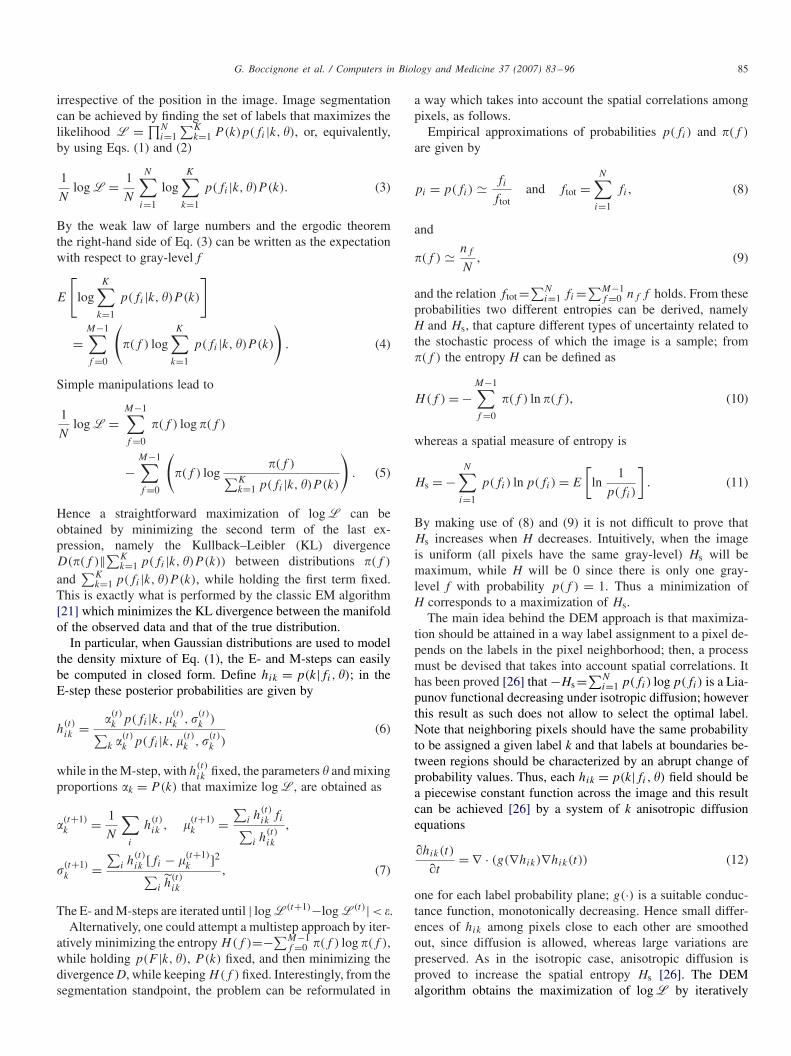
For showing results on gray-level images, we use an imageof a CT scan of the head at the level of the orbits, middle ear,and paranasal sinuses, Fig. 6(a) and an image of a radiographyof the hand, Fig. 6(b). In the case of the CT image, wheregray-level values represent average X-ray absorption distortedby noise and artifacts, the initially perceived complexity of theCT can be reduced by first identifying the major anatomical

G. Boccignone et al. / Computers in Biology and Medicine 37 (2007) 83–96 91

Fig. 6. Scalar images: (a) CT scan of the head at level of the orbits, middle ear, and paranasal sinuses; (b) Radiograph of a hand.

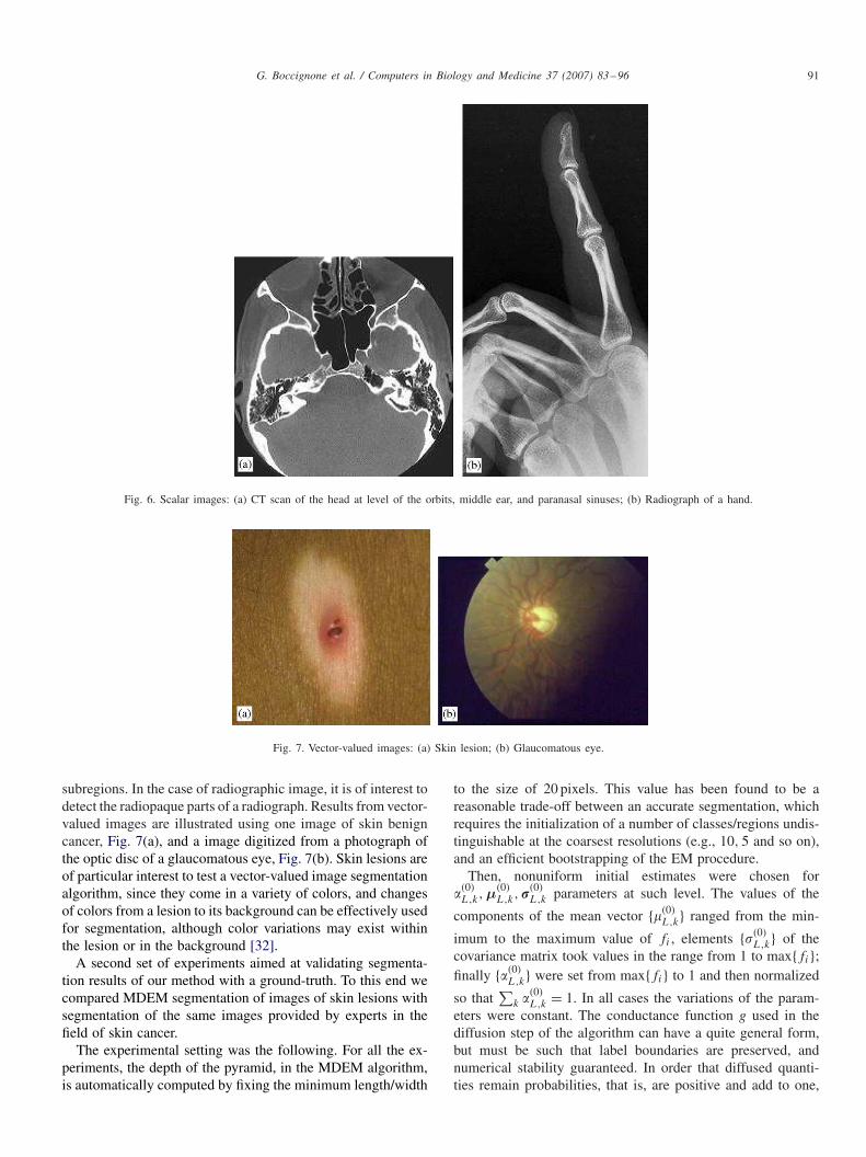
Fig. 7. Vector-valued images: (a) Skin lesion; (b) Glaucomatous eye.

subregions. In the case of radiographic image, it is of interest todetect the radiopaque parts of a radiograph. Results from vector-valued images are illustrated using one image of skin benigncancer, Fig. 7(a), and a image digitized from a photograph ofthe optic disc of a glaucomatous eye, Fig. 7(b). Skin lesions areof particular interest to test a vector-valued image segmentationalgorithm, since they come in a variety of colors, and changesof colors from a lesion to its background can be effectively usedfor segmentation, although color variations may exist withinthe lesion or in the background [32].

A second set of experiments aimed at validating segmenta-tion results of our method with a ground-truth. To this end wecompared MDEM segmentation of images of skin lesions withsegmentation of the same images provided by experts in thefield of skin cancer.

The experimental setting was the following. For all the ex-periments, the depth of the pyramid, in the MDEM algorithm,is automatically computed by fixing the minimum length/width

to the size of 20 pixels. This value has been found to be areasonable trade-off between an accurate segmentation, whichrequires the initialization of a number of classes/regions undis-tinguishable at the coarsest resolutions (e.g., 10, 5 and so on),and an efficient bootstrapping of the EM procedure.

Then, nonuniform initial estimates were chosen for�(0)L,k, µ

(0)L,k, �

(0)L,k parameters at such level. The values of the

components of the mean vector {�(0)L,k} ranged from the min-

imum to the maximum value of fi , elements {�(0)L,k} of the

covariance matrix took values in the range from 1 to max{fi};finally {�(0)

L,k} were set from max{fi} to 1 and then normalized

so that∑

k �(0)L,k = 1. In all cases the variations of the param-

eters were constant. The conductance function g used in thediffusion step of the algorithm can have a quite general form,but must be such that label boundaries are preserved, andnumerical stability guaranteed. In order that diffused quanti-ties remain probabilities, that is, are positive and add to one,

92 G. Boccignone et al. / Computers in Biology and Medicine 37 (2007) 83–96

Fig. 8. CT image segmentation results. From left to right, the original image and segmentation results of DEM, EM, split-and-merge, iterative entropythresholding, MDEM methods. Regions are coded with their average gray-value.

Fig. 9. Hand radiograph segmentation results. From left to right, the original image and segmentation results of DEM, EM, split-and-merge, iterative entropythresholding, MDEM methods.

a suitable normalization must be provided after each iterationstep; to this end, the functions h

(t)ik are renormalized so that

their sum is one after each iteration [31]. In our experimentswe set g(∇hik)=|∇hik|−9/5, while the values of , the numberof T (l) iterations of (18) performed at level l is automaticallyset as T (l)= 3× (1+ L− l), L being the maximum depth ofthe pyramid. The number of classes, K, was chosen to accountfor the classes to be determined in each experiment, with re-spect to different types of images, while convergence of thealgorithm was controlled by � = 0.1. For all the experiments,the same setting was used for EM, DEM and MDEM algo-rithms. The number K of classes automatically determines thenumber of thresholds Nt = K − 1 to be iteratively computedfor entropy thresholding (e.g., 2 thresholds t1 and t2 are neededto discriminate among 3 classes of regions).

Fig. 8 shows the results obtained on the CT image usingDEM, EM, split-and-merge, iterative entropy thresholding andMDEM by considering K=3 classes; regularization parameterof anisotropic diffusion was set as = 0.05. For the split-and-merge method, the threshold value �th = 1000 was experimen-tally chosen because providing the best performance.

It can be noted that DEM and MDEM achieve the mostreliable segmentations, but the latter is more precise in dis-carding small spurious regions, due to the multiresolutionanalysis. Worst performance is shown by the standard split-andmerge method, which is also outperformed by the thresh-olding method, though the latter exhibits higher sensitivityto noise.

Results obtained for the hand radiography are summarizedin Fig. 9. In this case K = 6 classes were taken into account;

G. Boccignone et al. / Computers in Biology and Medicine 37 (2007) 83–96 93

Fig. 10. Skin lesion segmentation. From left to right, the original image and segmentation results of DEM, EM, split-and-merge, MDEM methods. Regionsare coded with their average color value.

Fig. 11. Skin lesion contour: from left to right, original image, contours traced by a specialist, contours extracted after MDEM segmentation.

Fig. 12. Glaucoma image: (a) from left to right, original image, DEM, EM, Split and Merge, MDEM; (b) Contour of the Cup and the Disk of the Glaucoma.

anisotropic diffusion parameter was set as = 0.01. The split-and-merge method, was run with �th = 1000. Results achievedshow the same ranking among the considered methods as inthe previous experiment, in terms of quality of segmentation.

In the skin lesion case (Fig. 10) we have compared the meth-ods considering K = 4 classes (three main region classes plusone class for outliers), = 0.1 and the split-and-merge methodwas run with �th = 300.

Note that for this specific case the classical EM performsbetter than DEM in terms of spatial precision, because ofover-smoothing in the diffusion step. However, the MDEM al-gorithm is able to constrain smoothing due to multiresolutionanalysis. Interestingly enough, split-and-merge performanceon vector-valued images is higher than its performance on

gray-scale since variance is jointly taken into account over thedifferent channels.

To better appreciate the result obtained by MDEM, inFig. 11, the ground truth (marked contours) found by an expertin the field of skin cancer, where a lesion boundary potentiallyexists, is compared with the contour automatically traced viaedge detection performed on the segmented region.

The last example of this set of experiments (Fig. 12) showsresults in the case of an image of the eye fundus. In this casea glaucoma is present. We used K = 6 classes, = 0.1 and thesplit-and-merge method was run with �th = 200. Segmentationresults are illustrated in Fig. 12(a). Note that glaucoma is aneuropathy for which the evaluation of optic disk morphometrycan be of cardinal importance. For instance, the measure of the

94 G. Boccignone et al. / Computers in Biology and Medicine 37 (2007) 83–96

Fig. 13. Skin lesion segmentation results: (a) Original: from left to right, images 1–3 represent atypical lesions, 4 and 5, malignant lesions; (b) Ground truth(lesion boundaries manually traced); (c) boundaries automatically detected after MDEM processing and overlaid with the original.

Fig. 14. Skin lesion segmentation results: (a) Original: from left to right, the images represent benign lesions; (b) Ground truth (lesion boundaries manuallytraced); (c) boundaries automatically detected after MDEM processing and overlaid with the original.

cup to disk ratio is a widely accepted figure of merit. Thus, tobetter appreciate segmentation results, in Fig. 12(b) boundariesof the cup and the disk have been extracted from the segmentedimage and overlaid on the original, to show how this preliminary

step may allow easy computation of such ratio, when followedby simple circle fitting.

Eventually, we present some examples from a second setof experiments performed on images of pigmented lesions

G. Boccignone et al. / Computers in Biology and Medicine 37 (2007) 83–96 95

(either benign, atypical, malignant). To analyze such lesions itis necessary to accurately locate and isolate the lesions. Thus,results obtained by the MDEM algorithm have been comparedwith ground truths traced by experts in the field of skin cancer(Figs. 13 and 14). For ease of comparison, the contours of thesegmented regions have been extracted via edge detection andoverlapped onto the original image. Parameter settings werethe same as in the case presented in Fig. 11.

4. Final remarks

MDEM is a novel scheme that results in a simple but effec-tive segmentation algorithm for color images that: (1) retainsthe appealing characteristics of a feature clustering based ap-proach; (2) takes into account spatial constraints while avoid-ing complex schemes such as MRFs; (3) it operates within amultiresolution framework, in order to reliably define regionsof interest and efficiently perform required computations.

Note that the MDEM algorithm is different from previouslyproposed related methods. For instance, different approacheshave tried to incorporate within the EM algorithm a prior termin order to maximize a log-posterior probability instead of log-likelihood, thus leading to quite complex EM steps [23,24]. Onthe other hand, Haker et al. [31], have suggested to compute aninitial posterior probability map, through some kind of prelim-inary classification (e.g., clustering), followed by anisotropicdiffusion performed on such initial map in order to diffuse spa-tial constraints among probability sites; clearly, in this way finalresults strictly depend upon the goodness of the initial labeling.Here, we follow a different approach: we operate on the max-imization of the log-likelihood function, and spatial context isimplicitly accounted for along maximization via diffusion. Fur-ther, in order to take advantage of the structure of the image asrepresented at different scales, this methods has been carriedout in a multiscale framework, thus yielding an accurate seg-mentation, without unduly increasing the computational load.

Here it as been assumed K fixed, in that we are not concernedwith the problem of model selection. In general, this problemcould be tackled by resorting to BIC or Akaike’s informationcriteria [20]. However, this may not be necessary for biomedicalimages, since, depending on the application, the value of Kis often assumed to be provided by prior knowledge of theanatomy being considered.

As a result we obtain a simple iterative segmentation algo-rithm which can be easily interpreted in terms of a multiresolu-tion competition/cooperation scheme: at each resolution levelof the pyramid, the E- and M-steps can be seen as an individualsite competition between the k different label planes, while theinterleaved diffusion step can be considered as a cooperationstep within sites on the same plane.

With respect to the computational load, the whole algorithmis slightly slower than the EM procedure. Currently, it takes 30 sfor a 256× 256 2D image, using an Intel PIV 3.4 GHz proces-sor, equipped with 2 GHz RAM, under Windows XP operatingsystem.

Finally, simulations show that the method performs quitewell on a variety of medical images either with respect to more

standard methods or also techniques specifically designed foran application (for instance, our skin lesion segmentation re-sults can be compared with examples provided by Xu et al. [32]and available at www.cs.wright.edu/people/faculty/agoshtas/paper_fig.htm), and it is flexible enough to be used in a widerange of applications.

5. Summary

In the work presented here image segmentation of vector-valued images is carried out within a multiresolution frame-work. A multiscale representation is provided by Gaussianpyramids defined in the YCrCb color space, one for each colorchannel, and segmentation is performed in a hierarchical fash-ion, starting form the coarsest representation, so that resultsat a scale provide initial condition to segmentation in the nextlower (finer) scale; this propagation of information from coarseresolution levels makes significant objects/regions in the imagemore relevant respect to weak textures and noise. Also, pyra-mids provide an efficient tool to reduce the iterations necessaryto maximize the likelihood while optimizing the diffusion step,which, at each iteration acts upon a sub-sampled version of theprobability maps. At each scale segmentation is obtained viaan expectation–diffusion–maximization loop in which standardexpectation–maximization is coupled with a an anisotropic dif-fusion of the posterior probabilities of label assignment; thisway MDEM takes into account spatial correlations in the image.The new approach has been validated on a variety of medicalimages and through comparisons with more standard methods.

References

[1] L. Lucchese, S.K. Mitra, Color image segmentation: A state-of-the-artsurvey, Proceedings of the Indian National Science Academy (INSA-A),67, New Delhi, India, March 2001, pp. 207–221.

[2] J.S. Duncan, N. Ayache, Medical image analysis: progress over twodecades and the challenges ahead, IEEE Trans. Pattern Anal. Mach.Intell. (PAMI) 22 (2000) 85–106.

[3] D.L. Pham, C. Xu, J.L. Prince, Current methods in medical imagesegmentation, Annu. Rev. Biomed. Eng. 2 (2000) 315–337.

[4] S. Pohlman, K.A. Powell, N.A. Obuchowski, W.A. Chilcote, S.G.Broniatowski, Quantitative classification of breast tumors in digitizedmammograms, Med. Phys. 23 (1996) 1337–1345.

[5] I.N. Manousakas, P.E. Undrill, G.G. Cameron, T.W. Redpath, Split-and-merge segmentation of magnetic resonance medical images: performanceevaluation and extension to three dimensions, Comput. Biomed. Res. 31(1998) 393–412.

[6] J.J. Koenderink, The structure of images, Biol. Cybern. 50 (1984) 363–370.

[7] S. Mallat, A Wavelet Tour of Signal Processing, Academic Press, NewYork, 1998.

[8] P.J. Burt, E.H. Adelson, The Laplacian pyramid as a compact imagecode, IEEE Trans. Commun. 9 (1983) 532–540.

[9] S. Geman, D. Geman, Stochastic relaxation, Gibbs distributions, and theBayesian restoration of images, IEEE Trans. Pattern Anal. Mach. Intell.(PAMI) 6 (1984) 721–741.

[10] K. Held, E.R. Kops, B.J. Krause, W.M. Wells, R. Kikinis, H.W. Muller-Gartner, Markov random field segmentation of brain MR images, IEEETrans. Med. Imaging 6 (1997) 878–886.

[11] T. McInerney, D. Terzopoulos, Deformable models in medical imageanalysis: a survey, Med. Image Anal. 1 (1996) 91–108.

[12] P. Perona, J. Malik, Scale-space and Edge Detection Using AnisotropicDiffusion, IEEE Trans. Pattern Anal. Mach. Intell. 12 (1990) 629–639.

96 G. Boccignone et al. / Computers in Biology and Medicine 37 (2007) 83–96

[13] D. Geiger, A. Yuille, A common framework for image segmentation, Int.J. Comput. Vision 6 (1991) 401–412.

[14] D. Mumford, Bayesian rationale for the variational formulation, in: B.M.ter Haar Romeny (Ed.), Geometry-Driven Diffusion in Computer Vision,Kluwer Academic Publishers, Dordrecht, 1994, pp. 135–147.

[15] P.K. Sahoo, S. Soltani, K.C. Wong, A Survey of Thresholding Techniques,Comput. Vision, Graphics, Image Process. 41 (1988) 233–260.

[16] C. Lee, S. Hun, T.A. Ketter, M. Unser, Unsupervised connectivity-basedthresholding segmentation of midsaggital brain MR images, Comput.Biol. Med. 28 (1998) 30–38.

[17] G. Boccignone, A. Chianese, A. Picariello, Multiresolution spot detectionvia entropy thresholding, J. Opt. Soc. Am. A 17 (7) (2000) 1160–1171.

[18] G. Boccignone, A. Chianese, A. Picariello, Computer Aided Detectionof Microcalcifications in Digital Mammograms, Comput. Biol. Med. 30(2000) 267–286.

[19] R.O. Duda, P.E. Hart, D.G. Stork, Pattern Classification, Wiley and Sons,New York, 2001.

[20] D.J.C. MacKay, Information Theory, Inference, and Learning Algorithms,Cambridge University Press, UK, 2003.

[21] A.P. Dempster, N.M. Laird, D.B. Rubin, Maximum likelihood fromincomplete data, J. R. Stat. Soc. 39 (1977) 1–38.

[22] T.J. Hebert, Fast iterative segmentation of high resolution medicalimages, IEEE Trans. Nucl. Sci. 44 (1997) 1362–1367.

[23] S. Sanjay-Gopal, T.J. Hebert, Bayesian pixel classification using spatiallyvariant finite mixtures and the generalized EM algorithm, IEEE Trans.Image Process. 7 (1998) 1014–1028.

[24] Y. Zhang, M. Brady, S. Smith, Segmentation of brain MR images througha hidden Markov random field model and the expectation–maximizationalgorithm, IEEE Trans. Med. Imaging 20 (1) (2001) 45–57.

[25] G. Boccignone, M. Ferraro, P. Napoletano, Diffused expectationmaximisation for image segmentation, Electron Lett. 40 (2004)1107–1108.

[26] J. Weickert, Applications of nonlinear diffusion in image processing andcomputer vision, Acta Math. Univ. Comenianae 70 (2001) 33–50.

[27] G. Wyszecki, W.S. Stiles, Color Science-Concepts and Methods,Quantitative Data and Formulas, Wiley, New York, 1982.

[28] I. Pitas, Digital Image Processing Algorithms, Prentice-Hall International,London, U.K., 1993.

[29] G. Boccignone, M. Ferraro, An information-theoretic approach tointeractions in images, Spatial Vision 12 (1999) 345–362.

[30] D.A. Forsyth, J. Ponce, Computer Vision: A Modern Approach, Prentice-Hall International, London, UK, 2002.

[31] S. Haker, G. Sapiro, A. Tannenbaum, Knowledge-based segmentationof SAR data with learned priors, IEEE Trans. Image Process. 9 (2000)299–301.

[32] L. Xu, M. Jackowski, A. Goshtasby, D. Roseman, S. Bines, C. Yu, A.Dhawan, A. Huntley, Segmentation of skin cancer images, Image VisionComput. 17 (1999) 65–74.

Giuseppe Boccignone received the Laurea degree in theoretical physics fromthe University of Torino, Torino, Italy, in 1985. In 1986, he joined OlivettiCorporate Research, Ivrea, Italy. From 1990 to 1992, he served as a ChiefResearcher of the Computer Vision Lab at CRIAI, Naples, Italy. From 1992to 1994, he held a Research Consultant position at Research Labs of Bull HN,Milan, Italy, leading projects on biomedical imaging. In 1994, he joined theDipartimento di Ingegneria dellInformazione e Ingegneria Elettrica, Universityof Salerno, Salerno, Italy, where he is currently an Associate Professor ofComputer Science. He has been active in the field of computer vision, imageprocessing, and pattern recognition, working on general techniques for imageanalysis and description, medical imaging, and object-oriented models forimage processing. His current research interests lie in active vision, theoreticalmodels for computational vision, medical imaging, image and video databases.He is a Member of the IEEE Computer Society.

Paolo Napoletano received the Laurea degree in telecommunication engi-neering from the University of Naples Federico II, Naples, Italy, in 2003.He is currently working toward the Ph.D. degree in information engineeringat the University of Salerno, Salerno, Italy. His current research interests liein active vision, theoretical models for computational vision, medical imag-ing and image processing. He is a Student Member of the IEEE ComputerSociety.

Vittorio Caggiano received the Laurea degree in electronics engineering fromthe University of Salerno, Italy, in 2004. He is currently working toward thePh.D. degree in computer science and engineering at the University of NaplesFederico II, Naples, Italy. His current research interests are in the field ofactive vision, theoretical models for computational vision, medical imaging,image and video databases. He is a Student Member of the IEEE ComputerSociety.

Mario Ferraro received the Laurea degree in theoretical physics from theUniversity of Turin (Italy) in 1973. He has worked in Universities in England,Canada, Germany and United States, carrying on research on fuzzy setstheory, human vision, invariant pattern recognition and computational vision.Presently he is associate professor of Physics at the University of Turin. Hisresearch interests include image and shape analysis, cellular biophysics andthe theory of selforganising systems.