&AC-PUB-342 Au&St 1967

ASYMPTOTIC THEORY OF BEAM BREAK-UP

IN LINEAR ACCELERATORS*

W. K. H. Panofsky and M. Bander** Stanford Linear Accelerator Center

Stanford University, Stanford, California

(To be submitted to Review of Scientific Instruments)

* Work supported by U. S. Atomic Energy Commission

** Now at University of California, Irvine, California

I

I. GENERAL DESCRIPTION OF OBSERVED PHENOMENA

The observed beam current of the SLAC SGO-section linac appears to obey the

results of independent particle dynamics at low intensities. However, as was first

observed on April 24, 1966, the pulse length of the transmitted beam appears to

shorten provided the beam current exceeds a threshold value at a given distance

along the accelerator; the g-rester the distance, the lower the threshold. This general

behavior is illustrated in Fig. 1. Further tests clearly indicated that the phenom-

enon responsible is the sudden onset of a radial progressive instability conven-

tionally called beam break-up (BBU).

Observation of radial instability in high current linear accelerators is not

new,lW6 and the phenomenon has been conclusively associated with the excitati.on

of transverse deflecting modes. However, one should clearly recognize that we

are dealing with two quite distinct mechanisms by which such modes can lead to an

amplifying action. The first mechanism discussed in the above references results

from the negative group velocity of the TEMll mode of the conventional disk-loaded

structure. This negative goup velocity will feed transverse energy from the end of

a given acceleratin, m section t.o the front, thus leading to the regenerative action

involved in the “backward-wave oscillator. ” This phenomenon of regeneration

within a given section characteristically occurs at currents of several hundred

milliamperes at pulse lengths of several microseconds. The second mechanism

which is dominant in a multiscction relatively low current accelerator (such as

SLAC or the liharkov 2-GeV accelcrator)7involvcs amplification from section to

section, coupled only by the electron beam without backward propagation of elcctro-

magnetic energy.

- 1 -

In this paper we will give the theory of the second mechanism only, which is

the dominant cause of the BBU phenomena occurring at SLAC. As will be seen, this

mechanism is very gcncral, being quite independent of the d&ailed. structure of the

accelerating sections.

II. THE MULTICAVITY MODEL

A. The Model

We will represent each section of the accelerator by a single cavity; the cavity

geometry constitutes a free parameter which can be choskn to fit the experimental

behavior.

We will assume:

(a) Only one resonant mode at a frequency w0 and loss factor Q is of

significance.

(b) The cavity has axial symmetry and the axial electric field vanishes

along the axis of symmetry.

(c) The rate of build-up of oscill.ation giving rise to the radial modulation

of the beam is small compared to w 0’ th

Consider a particle of charge e to cross at a t.ime t the n of N cavities

at a distance x from the z-axis, taken to be an axis of symmetry. Let L be the

distance between cavities, and let the particle velocity be v M c = 1 (see Fig. 2).

B. Equation of Motion

Let the electric field F in the n th cavity be derivable from a vector potential

A, and let each cavity be excited near a single resonant frequency uo. We obtain

from the deflection theorem* for the change in transverse momentum px in the

nth cavity :

Apx = e s

aAZ - dz 3X

(1)

-2 -

This transverse momentum Ap, results in a difference in displa6ement of

(Apx/mor) L bet7veen the (n f l)th and nth cavity where moY is the particle

energy. We can thus write a difference equation which can be approslmated as a

transverse differcnt,ial equation of motion as follows :

c. Exe itation of Cavities

Equation (2) gives the radial equation of motion as governed by the transverse

gradient of the longitudinal component of the vector potential and hence the electric

field. No special assumptions as to mode structure are assumed. If the particle

passes at a distance x (assumed constant in each cavity) from the symmetry axis,

then $11 general, work is done against the longitudinal field.

Each cavity excited at a frequency w near w. loses energy U to the current

j at the rate j J

j? + d; and loses energy to wall losses at the rate w U/Q. The

rate of build-up is therefore given by (averaged over many cycles as designated by the

symbol)

a=-j ~s&-!$. at s

(3)

If the field z = 7 on the axis and varies linearly from. the axis, J- z l dp can

be approximated by: -

J J aEz $-.d;-x _ dz ax

(4)

where x is the transverse coordinate at which the beam carrying the current j

passes from the axis. The cavity excitation is thus proportional to x; on the other

hand the cavity, once excited, will affect the motion in x according to Eq. (2).

-3-

As a result the beam will receive a transverse structure so that x will be modu-

lated at a frequency w near wO.

Note that the field integrals appearing in Eq. (2) and in Eq. (4) are simply

related if we can assume that oscillations take place near w = wO and that the

rates of build-up or damping

that all field amplitudes vary

placement to vary as e +iwt

amplitudes carrying both the

Using this convention we

are slow relative to w 0’ We adopt the convention

+iwt as e and that we consider the transverse dis-

also. The quantities x, E, A thus become complex

phase and the (slowly varying) amplitude information.

can write the field integral in (4)) using Ez = - aAz/at :

s

aE -? dz $5 - iw

s

aAZ I(t) = - dz (5)

3X 3X

giving the equations of motion and the energy build-up equations

a ax ( 1

ieL dn Ydn =-0 I m W

au wU=-J$j

at' Q .

(6)

In general U and I are related quadratically through a (generally complex)

impedance. In general we can write

(7)

and

(8)

(9)

where * denotes the complex conjugate and Re the real part. Hence (7) becomes, * * aI noting that I g + I at = 21* aI at :

31 ~+$p4~x.

-4 -

(10)

Combining (6) and (10) we obtain;

as the basic clifferential equation governing the build-up of the instability.

The impedance constant Ii can be related qualitatively to the dimensions of

the cavity. Let P be the length of the cavity which can be interpreted as an effective

“interaction length” in the actual case. We have dimensionally:

where a is a radial dimension of the cavity. More quantitatively,

cylindrical cavity of ra.dius a = 3. 83/~

(12)

for a simple

EZ =, ff Jl ( KP) cos Q

where the symbols have their usual meaning. The integral. in (12) then gives

u = a4

The constant Ii in Eqs. (8) - (11) is thus:

I< = (~~/r)/l81

Let us measure beam intensity in terms of the quantity J = number of

particles/set (or number of particles/unit length since we take v “N c = 1).

Hence we can write Eq. (11) as

(13)

(14)

(16)

-5-

I

where

P = w/zQ

and

2 c = 7.2 e Es!

“0 a4 (17)

is a dimensionless constant expressed in terms of the classical electron radius

rO =e =: 2. 8 X lo-l3 cm .

D. Physical Discussion -

The build-up of oscillation is governed by the integrals of Eq. (16); blow-up

will be dominated by that frequency w which will maximize the build-up rate.

Let us understand some of the qualitative features of these equations.

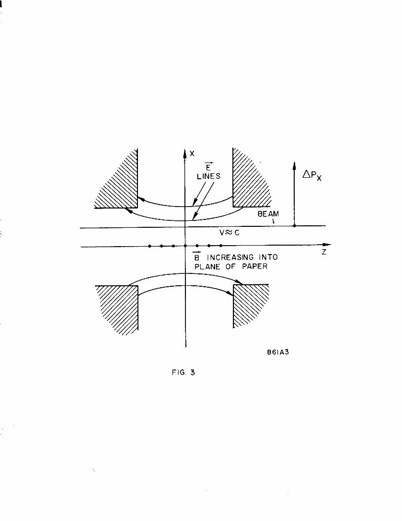
The field configuration in the deflecting mode has the qualitative configuration

shown in Fig. 3. The 2.bove analysis shows that thedetails of the fieldconfiguration are

of minimum sig>Gficance since the same integral I over the fields governs both

the tra.nsverse momentum imparted to the particle as well as the coupling of the

particle in “driving” the field build-up, Equation (6) shows that the transverse

momentum Apx is in phase quadrature (leading) with the field integral I.

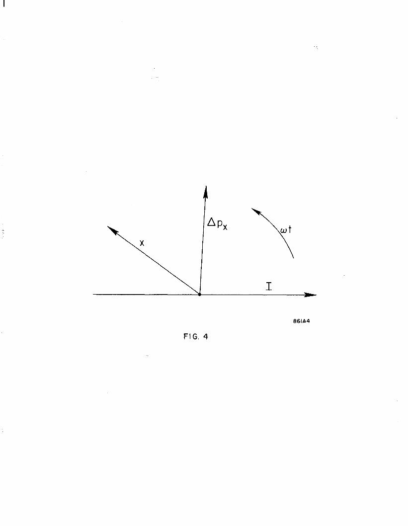
According to Eq. (10) a linear combination of the field integral I and its rate

of build-up is 180’ out of phase with the driving displacement x. On the other hand

x and Ap, must have a common in-phase component if the oscillations are to

grow. Therefore for maximum build-up the phase of x will be somewhere between

the phase of Ap, and - I, as shown in Fig. 4.

E. Solution by Laplace Transform Using the Method of Steepest Descent

In this section we will study the solution of the equation (16) where y is a

given function of n .

-6 -

I

Let us try the Laplace transform solution, using an appropriate contour c ,

x(n,t) = e -Pt J f(w) 2” 6-l (18) C

in Eq. (16). The function f(n,p) satisfies

p (yf’)’ + iCJf = 0 (1%

where ’ denotes differentiation with respect to 11. We can integrate this equation

by assuming adiabatic variation of y with n (WKB approximation). The result is

f(w) - Y -l/4 l/2 ~-l/2

g (20)

where

since the general WI<13 solution of the equation (Rf’)’ + Bf = 0 is

fN -& exp[%iF JD/hdn’] . (22)

The i term in the exponent of Eq. (20) is carried from Eq. (16) and governs

the phase of the space harmonic in x at the frequency w relative to the phase

of the electric field in each cavity, as discussed previously. Hence the general

solution is

x(n,t) = eSPt J 1-1 t $ i [iCJ/p]1’2 g C

(23)

where the weighting function w&) depends on the starting conditions, We chose

the root giving a positive real part in the exponent.

Evaluation of the function w@) in terms of specific stzrting condition, such

as a unit disturbance in x occurring at n = n 0

at a fixed time, is quite

- 7 -

I

straightforward, but evaluation of the inverse Laplace integral, Eq. (231, in general

is not possible in closed analytical form.

Among such starting sources are:

Shot noise in beam

Shock excitation through misalignments

Thermal noise in early sections

Noise or spurious signals from klystron power sources

Electrical discharges in high microwave fields

Present experimental evidence is not conclusive as to which of these initial driving

terms are important. However, the question of largest practical interest is the

dependence of x on the various physical parameters (current, length of current

pulse, number of cavities) once a “blow-up” of x, sufficiently large to lead to

beam loss, has occurred. Such loss requires a large ( lo7 to 10’) amplification.

For this purpose an asymptotic solution is adequate which can be generated by the

method of steepest descent.

The “saddle point” of the exponent in Eq. (23) is at one of the roots p = 6

of the equation

d f (CJ) 112 dT

which occur at:

(24)

(25)

leading to a value 8 (E ) of the exponent of Eq. (23) of

e(E) = 2 l/3 $3 (CJ)

l/3 g2/3 3 .(1/2 +2/3 n)A 3

(26) 2

where n is any integer.

-8 -

We chose that value of ii for which E has the greatest real part., i. e. , for

which blow-up occurs at the maximum rate, This gives n = 2 or

O(E) = 3(2 1’3/4)(& - i)(CJt)‘j3 g2’3 =(1.64 - 0.94i)(CJt)1’3 g2/” (27)

The appropriate contour passes through the “saddle-point” 1-1 = t along a

direction of “steepest descent ,‘I i. e. , along a direction to make 0 0-1) a greatest

maximum S If we expand 0 Q ) about 1-1 = E , we can put:

O&l) = 0 (E) + $ ((1 - q2 0” (6)

Differentiation of (26) gives :

8 ‘ , tE) = (3,21/3)(CJ)-1/3 t513 b,-2'3 ,i7r'G

(28)

(29)

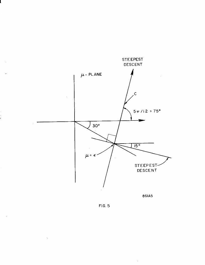
Let the argument of the contour c of steepest descent when passing through

p = E be $, i.e. , let 1-1 - 6 --; P e i+

where p and II, are real, The argument of

u _ e)2 0 1 1 tE) = p2 1 0 ’ l (E) 1 ei(21’.t”/6) (30)

is -x along the path of steepest descent, or + = 5 r/12. The appropriate

contour is shown in I?ig. 5 . The function of (n,p) thus falls off steepest in both

direct.ions along c away from the real axis. This leads to a useful approximation

if the cxponcnt is large, ’ i. e. , if “blow-up! has largely progressed.

The a.symptotic solution is then given by evaluation of the integral (23), using

Eqs. (26), (28), and (29); and obtain:

x(n,t) = xO(n,t) cxp I?( 2l/3/4) (fl-i)(CJt)l’3g2’3 -pt.}

where x0(n) t) is a relatively slowly varying function given by

x0(“, t) sz J l/6 t-5/6 g1/3 ?-l/4

(32)

-9 -

?‘he growth is thus controlled by the exponent

1.64 C1’3 tJg2 1’3 ( )

(33)

in the highly transient break-up observed at SLAC, where the term /3t is small

compared to the present term.

For a constant t’blow-up factortl we thus obtain the basic scaling law:

(J t) 8’ = constant (34)

Hence the total. charge (J t) per pulse which can be accelerated to a specified

point along the accelerator under a given acceleration program y(n) within a

li.miting blow-up factor is constant, i. e. , independent of pulse length.

Let us evaluate the integral g if we accelerate from n0 to n1 at a uniform

energy gain y’ and coast from there to section n 2. We obtain:

52

g = s Y -l/2

2 dn’ = ~‘1/2 m - n0 + +m (“2 -nl) (35)

nO

For constant accelerati.on (no coasting ) and nl >> no we obtain the simple

scaling law,

Jt nl/‘y’ = constant (36)

while for l’pure” coasting from n 1 to n2 ,*at an energy yc we obtain

Jt (n2 - nlvyc = constant (37)

Numerical comparisons of these relations with experience is good and has been

discussed elsewhere. 9 Suffice it to say that reasonable agreement is obtained with

an exponent of about 20 leading to beam loss through BBU.

- 10 -

The stecpcst descent calculation leads to valid results only if the exponent is

large, The error can be estimated by estimating the variation of xotn, t) as given

by Eq. (32) over the range of interest. For numerical situations of interest this

might add a correction of no more than 20% to the exponent.

F. ,Solution by Iteration -I_ -__

The steepest descent solution is purely asymptotic and thus canaot be linked ID

the starting condition, Let us now examine the solution of the basic differential

equation (16) under the boundary conditions corresponding to a b-function impulse

a.t t = T, i. c. ,

x(11 = no,t) = 6(t -T)

2 (11 =no,q = 0

As mentioned above, the exponenti-tl factor exp( - p t) is always factorable; we

can thus write a first integral by putting

y(n,t) = x(n,t) exp(pt) (39)

where y(n, t) satisfies

f--[y g (n,t)] -t iCJL y(n,t’) dt’ = 0, (40)

and where the boundary conditions are

Y (n = no,t) = 6(t - T) e PT

(41)

24 (n = no,t) = 0

- 11 -

We again make the WKB approximation. Let

YW) = .A F [g@), t] crd 4

(42)

If we neglect terms of the order of (dr/dn)2 and (d2y/dn2), (which is exact

in the absence of acceleration) we find that F(z, t) satisfies

a2 t

- F(z,t) = - iCJ az2 s

F(z,t’) dt’

-03

F(O,t) = y. 1’4 epT 6(t - T)

e PT

Incorporating these boundary conditions we obtain an integral equation for

F(z,t) :

F(z,t) = - iCJi dt’j dzf ‘dz” F(z”,t’) + 4s zePT 6(t -T)+rki4 6(t -T) epT

-00 0 0 0 (44)

The solution Eq. (7) may be found by iteration:

+O(t-T)epTg (-iCJ)j el; X . j=l

( l/4 z2j X I!- + VI z2 jtl

, (45)

W)! p 0 (2j+l)! )

where 6 (t - T) is a unit step function.

- 12 -

I

Using the definition for I. n

given by Eq. ! (Zl), we may trace back to obtain a solution for x(n, t) :

For the coasting (non-accelerating) case this simplifies to

a3 2cJj-1

x(n, t) = e +(t-T) + 0(t -T) y (n -n0)2 (-i)j y. I 1 (4 7)

C (2j)! (j - l)!

Due to the appearance of (2j) 1 (j - 1) ! in the denominator, this series converges

very rapidly. For z2(t -T) - 3000, fifteen terms would be sufficient.

In Figs. 6 and 7, the numerical evaluati.on of the sums is presented. Let g(n),

YO’ and yb be as above. Note that the expansion parameter

S3 = CJ g2 (t - T) (48)

is the same as that appearing in the asymptotic calculation leading to Eq. (31).

Re-expressing Eq. (46) in terms of functions of s, we obtain:

e-Ptt-T) x(n,t) = [D

l/4 yo + --$ g(n) o ) c?(t-T) + 0(t-T)CJ g2

- 13 -

I

The amplitude functions A(s) and B(s) are shown in Fig. 6. Asymptotically

the functions behave as :

exp 3 ( 3/2

in agreement with the steepest descent solution Eqs. (27) and (31). Figure 7 gives

the phase functions 4(s) and q(s). The first term in Eq. (49) is generally negli-

gible since it represents the original impuke without build-up.

These figures (Fig. 6 and Fig. 7) can be used to construct by superpositon

any build-up pattern resulting from an initial disturbance x(t) at n = n 0’

G. Steady State Solution

If the pulse length is sufficiently long, equilibrium with the wall losses will

be reached. The basic differential equation (16) then reduces to

[ii& (Y=&) + iCJ]x = 0

This has the WKB solution [see Eq. (ZI)]

n

x(n) - (/3’rCJ)1’4 J

(iCJh9 “’ dn’

(50)

(51)

Ignoring a phase factor and multiplicative constants this gives a positive exponen-

tial solution, valid at a time t >> Q/U :

x(n) - [r(n)]-1’4 ew?[(QCJ/d’2 g(n)] (52)

This case is not of relevance to the SLAC accelerator since Q/w - 1 ilsec.

However, for a potential cryogenic accelerator permitting CW operation, the

steady state solution is of interest.

- 14 -

III. THE EFFECT OF TRANSVERSE FOCUSING

In the previou s sections we analyzed the general behavior of the BBU phenom-

enon in the absence of transverse forces other than those associated with the trans-

verse modes associated with the BBU itself. The actual accelerator contains a

series of strong focusing lenses to confine the beam; these will affect the BBU

llgain” of each section and their strength and distribution can be used to increase

the BBU current threshold by a significant amount.

The theory of the preceding section is completely linear; it is therefore easy

to indroduce the effect of linear focusing devices such as quadrupole or magnetic

solenoids; on the other hand it is difficu.lt to introduce either the effect of lenses

of higher than quadrupole order, or the effect of bunching into the theory; we note

however that to the extent that the bunch structure is incoherent with the frequency

of the BBU, longitudinal bunching will not affect the phenomenon.

On the basis of these remarks we can introduce the effect of linear transverse

focusing by introducing a term

yk’x (53)

into the basic differential equation (19), giving

($I)’ + -&‘f 1 + iCJf = 0 (54)

Here 2x/k(n) is the “betatron wavelengthft produced by the external focusing

sys tern produced by quadrupoles .

The Laplace transform solution (22) then becomes

iCJ/py + k (55)

- 15 -

The evaluation of this integral by the method of steepest descent is not possible

analytically. We can however obtain an approximate solution for “weak focusing”

corresponding to

k2 << CJ/E Y (56)

where 6 is given by Eq. (25). Carrying only linear terms in k2, the exponent

in Eq. (55) becomes:

S(p) =pt* 1 (."/'[cJ/~ ]1/2g+i’/2[~/CJ]i/2~/

where g(n) is given by (21) as before, and K i-s the integral

n

K(n) = i s

’ k y ‘1’ dn’

nO

cw

The saddle point occurs to order linear in K at the point ~1 = E given by:

c = (CJ) l/3 (gj2t)2/3 e-7i i/6 l _ (21/3/3j leg-1/3 (C Jt)-2/3 e- (2/3)ni

3 (59)

This leads to a value of the exponent 8 (6) given by:

O(r) = ;x 2 1’3 (g’CJt) l/3 e-(ri/6) _ 2-1/3 g1/3 K(CJt)-l/3 .d/6 (60)

The leading term agrees with Eq. (27) while the second term is a damping factor

proportional to the focusing integral IL The real part of Eq. (60) can be written

in the simple form:

Re [C (E )) = F 1 [ - y(( y-1’2dnj(l y”’ k2 dnjl (61)

where F = 1.64 (g2CJt) l/3 is the exponent in the absence of external focusing.

The current which will lead to a given value of BBU amplification will thus be

.I

- 16 -

increased by a factor f given by

(62)

This formula gives reasonable agreement with experiment for a value of F N” 20.

ACKNOWLEDGEMENT

The writers are greatly indebted to Dr. Richard Helm for important comments

and corrections .

- 17 -

REI’ERENCES

1. M. C. Crowley-Milling, “A 40-McV electron accelerator for Gcrnlnny,‘f

AEI Engineering 2, No. 2 (1962).

2. G. H. I-I. Chang, l’Pulse shortening in electron linear accelerators, 11 M. SC.

Thesi.s, University of California, Berkeley, California (19G4); see also

E. 1,. Chu, “A crude estimate of the starting current for linear accelerator

beam blow-up in the presence of an axial magnetic field, ‘1 Technical Note

No. SLAC-TN-66-17, ,Stanford Linear Accelerator Center, Stanford University,

Stanford, California (1966).

3. M. G. Kelliher and R. Beadle, Nature 187, 1099 (1.960).

4. H. Hirakawa, Jap. J. Appl. Phys. 3, 27 (1964).

5. T. R. Jarvis, G. Saxon, and M. C. Crowley-Mil.l.~lg, Proc. IEEE (London)

112, 1795 (1965).

6. P. B. Wilson, “A study of beam blow-up in electron linacs , I1 Report No.

HEPL-297 (Rev. A), High Energy Physics Laboratory, Stanford University,

Stanford, California (June 1963).

7. G. V. Voskresensltii, V. I. Koroza, Yu. N. Serebryakov, “Transverse

Instabilities of a Beam in a Linear Accelerator Prior to Increasing Injection

Current, I’ Uskoriteli (Accelerators), Vol. 8, p. 135, Moscow Institute of

Engineering Physics, Atomizdat, Moscow (1966), and

V. A. Vishnyakov, I. A. Grishaev, A. I. Zykov, L. A. Makhnenko, “A

Question Concerning the Rise of the Limit of Current in a Multisection Linear

Accelerator, ‘I Publication No. 309/VE-072, Academy of Sciences, Ukrainian

Soviet Socialist Republic Physics and Engineering Institute.

8. W.K.H. Panofsky and W. A. Wentzel, Rev. Sci. Instr. 27, 967 (1956).

9. 0. H. Altenmueller, E. V. Farinholt, Z. D. Farkas, W. B. Herrmannsfeldt,

H. A. Hogg, R. F. Koontz, C. J. Kruse, G. A. Loew and R. H. Miller, “Beam

Break-Up Experiments at SLAC, I1 Stanford Linear Accelerator Center, Stanford

University, Stanford, California, Proceedings of the 1966 Linear Accelerator

Conference, LA-3609, October 3 - 7, 1966.

I?IGUItE CAPTIONS

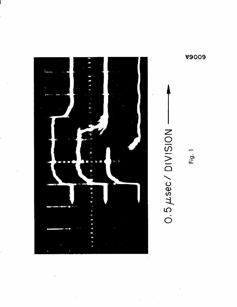
1. Current pulse shapes observed at the end of the accelerator shown for 3-peak

current amplitudes. Note the pulse shortening effect of beam break-up.

2. The single cavity model. The figure shows the notation used describing the

geometry of the nth cavity relative to the preceding and following unit. Each

cavity represents resonant excitation of a particular transverse mode of each

of the sections of the accelerator.

3. Field configuration in a typical transverse mode.

4. Phase relationships between transverse displacement x, transverse rnomen-

turn gain Apx , and the field integral I.

5. Location of the saddle point in t-he complex plane and the path of steepest descent.

6. The amplitudes of the functions A(s) and B(s) as defimd in Eq. (49).

7. The phases Z/J(S) and @ (s) as defined in Eq. (49).

z 0

w9009

ti .- u

-‘ A

w

-

n-l

n

FIG

. 2

n+l

-

g INCREASING INTO Z

PLANE OF PAPER

861A3

FIG. 3

npx

I

wt

\

86lA4

FIG. 4

STEEPEST DESCENT

p- PLANE

/ STEEPEST DESCENT

86lA5

FIG. 5

0.1: 01234567

I I I I 8 9 10 II 12 13 14

S 543-2-c

Fig. 6

I

0

W

lo

N

0

( S33U%lCl ) 3SVHd