Ambient Noise Rayleigh Wave Tomography Across Europe

Yingjie Yang, Michael H. Ritzwoller, Anatoli L. Levshin, Center for Imaging the Earth�s Interior

Department of Physics University of Colorado at Boulder,

Boulder, CO 80309-0390 USA, yingjie.yang@colorado.edu

and

Nikolai M. Shapiro

Laboratoire de Sismologie, CNRS IPGP, 4 place Jussieu 75005 Paris, France

Submitted to Geophysical Journal International

Revised on August 24, 2006

1

Summary

We extend ambient noise surface wave tomography both in band-width (10 sec - 50

sec period) and geographical extent (across much of Europe) compared with previous

applications. Twelve-months of ambient noise data from 2004 are analyzed. The data are

recorded at about 125 broad-band seismic stations from the Global Seismic Network

(GSN) and the Orfeus Virtual European Broad-band seismic Network (VEBSN).

Cross-correlations are computed in daily segments, stacked over one-year, and Rayleigh

wave group disperson curves from 8 sec � 50 sec period are measured using a

phase-matched filter, frequency-time analysis technique. We estimate measurement

uncertainties using the seasonal variation of the dispersion curves revealed in

three-month stacks. On average, uncertainties in group delays increase with period from

~3 sec to ~ 7 sec from periods of 10 sec - 50 sec, respectively. Group speed maps at

periods from 10 sec to 50 sec are estimated. The resulting path coverage is denser and

displays a more uniform azimuthal distribution than from earthquake-emitted surface

waves. The fit of the group speed maps to the ambient noise data is significantly

improved below 30 sec compared to the fit achieved with earthquake data. Average

resolution is estimated to be about 100 km at 10 sec period, but degrades with increasing

period and toward the periphery of the study region. The resulting ambient noise group

speed maps demonstrate significant agreement with known geologic and tectonic features.

In particular, the signatures of sedimentary basins and crustal thickness are revealed

clearly in the maps. These results are evidence that surface wave tomography based on

cross-correlations of long time-series of ambient noise data can be achieved over a broad

period band on nearly a continental scale and yield higher resolution and more reliable

group speed maps than based on traditional earthquake-based measurements.

2

1. Introduction

Traditional inference of seismic wave speeds in Earth�s interior is based on

observations of waves emitted by earthquakes or human-made explosions. In the past

decades, with the deployment of a large number of high-quality broad-band seismic

stations across the globe, there have been numerous tomographic studies performed on

both global and regional scales using the travel times of body waves, dispersion curves of

surface waves, and waveform fitting methods. Much information has been obtained about

the structure of Earth�s interior using these methods.

Surface wave tomography has proven particularly useful in imaging Earth�s crust

and uppermost mantle on both regional and global scales. Because they propagate in a

region directly beneath Earth�s surface, surface waves typically generate better path

coverage of the upper regions of Earth than body waves with the same distribution of

seismic stations. Surface waves at different periods are sensitive to Earth structure at

different depths, with the longer period waves exhibiting sensitivity to greater depths. By

measuring the dispersive character of surface waves, the structure of the crust and upper

mantle can be relatively well constrained. In Europe, many traditional surface wave

studies have been performed in the past, both at regional (e.g., Papazachos, 1969; Nolet,

1977; Mueller and Sprecher, 1978; Maupin and Cara, 1992; Stange and Friederich, 1993;

Vaccari and Panza, 1993; Pedersen et al., 1994; Lomax and Snieder, 1995; Pontevivo and

Panza, 2002; Levshin et al.2006) and continental scales (e.g., Panza et al., 1980; Patton,

1980; Snieder, 1988; Marquering and Snieder, 1996; Ritzwoller and Levshin, 1998;

Yanovskaya et al., 2000; Pasyanos, 2005; Pasyanos and Walter, 2002).

There are, however, basic limitations to earthquake-based surface wave tomography

independent of the number of broad-band stations available. First, due to the uneven

distribution of earthquakes around the world, seismic surface waves only sample certain

preferential azimuths. In addition, in aseismic regions surface wave dispersion can be

measured only from distant earthquakes. Second, it is difficult to obtain high-quality

3

short-period (<20 sec) dispersion measurements from teleseismic events due to intrinsic

attenuation and scattering along ray paths. It is, however, the short-period waves that are

most useful to constrain the structure of the crust and uppermost mantle. Third,

inversions of seismic surface waves require some information about sources, such as

earthquake hypocentral locations and moment tensors in some cases, which have a

substantial intrinsic inaccuracy, particularly for small events.

Some of the problems that beset traditional earthquake surface wave tomography

can be alleviated by observations made on diffuse wavefields (e.g., ambient noise,

scattered coda waves). Theoretical research has shown that, under the right circumstances,

the cross-correlation of records from two seismic stations provides an estimate of the

Green function between the stations, modulated by the spectrum of the noise source

(Weaver and Lobkis, 2001a, 2001b, 2004; Derode et al., 2003; Snieder, 2004; Wapenaar,

2004; Larose et al., 2005). Seismic observations have confirmed the theory using both

coda waves (Campillo and Paul, 2003; Paul et al., 2005) and ambient noise for surface

waves (Shapiro and Campillo, 2004; Sabra et al., 2005a) and crustal body waves (Roux et

al., 2005). Oceanic applications also appear to be feasible (Lin et al., 2006). The method

has been successfully applied to stations in Southern California to obtain high-resolution

surface wave tomography maps at short periods ranging from 7.5 to 15 sec (Shapiro et al.,

2005; Sabra et al., 2005b). The group velocity maps from these studies show a striking

correlation with geological units in California with low-speed anomalies corresponding to

the principal sedimentary basins and high-speed anomalies corresponding to the igneous

cores of the major mountain ranges. More recent applications have arisen across all of

California and the Pacific Northwest while tracking the growth of the Transportable

Array component of EarthScope (Moschetti et al., 2005), in South Korea at very short

periods (Cho et al., 2006), in Tibet (Yao et al., 2006), and elsewhere in the world.

This research has shown, therefore, that information about Earth structure between a

pair of seismic stations can be extracted by cross-correlating long time sequences of

4

seismic noise. With sufficient station density, cross-correlations of ambient seismic noise

promise to yield more homogenous sampling over study regions than earthquakes, to

provide information to shorter periods so as to improve constraints on crustal structure,

and partially to release seismologists from the dependence on earthquakes in surface

wave tomography.

The purpose of this paper is to determine whether ambient noise Rayleigh wave

tomography can be applied reliably on a nearly continental scale and extended to

intermediate periods up to ~50 sec. The study is based on data across Europe from 125

broad-band seismic stations from the Global Seismic Network (GSN) and the Virtual

European Broad-band Seismic Network (VEBSN). We compute broad-band

cross-correlations to produce estimated Green functions for all station-pairs using

one-year time-series. The assessment of the reliability of the measurements is based on

four primary criteria: (1) signal-to-noise ratio (SNR) of the cross-correlations, (2)

seasonal repeatability of the dispersion measurements, which is the basis for the error

analysis, (3) misfit of the measurements determined from tomography, and (4)

consistency of the estimated group speed maps with known structural features such as

sedimentary basins and crustal roots beneath mountain ranges. Group velocity curves

across Europe are measured from 10 to 50 sec period and we present group speed maps

from 10 to 40 sec period. The results are compared, whenever possible, to

earthquake-based measurements and maps produced earlier by the University of

Colorado at Boulder (CU-B) in order to quantify the relative merits of ambient noise and

earthquake tomography.

2. Data processing and group velocity measurements

Europe is an excellent region to test ambient noise surface wave tomography.

Broad-band seismic station coverage is dense across much of the continent, particularly

in its center, and the substantial a priori knowledge of geological structures allows us to

5

evaluate the reliability of the resulting group velocity maps. We have collected

continuous vertical-component seismic data from 125 stations including data from the

Global Seismic Network (GSN) and the Virtual European Broad-Band Seismic Network

(VEBSN) (Figure 1) over the 12 months of 2004.

The data processing procedure that is applied here is very similar to that discussed at

greater length by Bensen et al. (2006). Using vertical-component seismic data implies

that the resulting cross-correlations contain only Rayleigh wave signals. Data are

processed one day at a time for each station after being decimated to 1 sample per second

and are band-pass filtered in the period band from 5 to 150 sec after the daily trend, the

mean and the instrument response are removed. Data are then normalized in time and

whitened over the frequency-band of interest prior to cross-correlation. Spectral

whitening is a straightforward procedure, but the temporal normalization requires more

discussion.

Temporal normalization is a general phrase that describes a variety of methods used

to remove earthquake signals and instrumental irregularities from the time-series prior to

cross-correlation. At periods where earthquake signals are stronger than ambient noise,

roughly above about 20 sec period, some method of removing earthquake signals is

imperative. For this purpose, Shapiro et al. (2005) used one-bit normalization, which

generates a data stream composed only of the values 1 and -1, retaining only the sign and

disregarding the amplitude of the signal completely (Larose et al., 2004). Other

researchers have used different methods; for example, Sabra et al. (2005b) used a

truncation threshold for each station to clip seismograms. Based on observations of the

signal-to-noise ratio of the cross-correlations, we have come to prefer applying a

weighted running average on the envelope of each seismogram in the time domain, which

effectively removes earthquake signals while keeping much of the information on the

amplitude of the ambient noise. The process applied here computes the average of the

envelope of the seismogram over a normalization time interval, and weights the

6

seismogram by the inverse of this average at the center of the window. The width of the

normalization window determines how much amplitude information is retained. A

one-sec window is equivalent to one-bit normalization; while an infinitely long window

is equivalent to the original signal renormalized. After testing various time windows, we

find that a time window with width equal to half the maximum period of the band-pass

filter works well. The maximum period here is 150 sec, so the normalization window is

about 75 sec in duration. Normalization windows from 50 to 100 sec in duration produce

nearly indistinguishable results. This procedure of temporal normalization is found to

generate a somewhat higher SNR than 1-bit normalization, on average. In addition, the

procedure is more flexible, allowing, for example, the computation of the temporal

weights in a sub-band (e.g., 15 � 50 sec designed to remove earthquakes) but with

application to the broad-band signal.

After the time-series has been processed for each day, we then compute daily

cross-correlations in the period band from 5 to 150 sec between all station-pairs and then

stack the results into a set of three-month and one-year time series. The stacking simply

involves adding the daily cross-correlations without weights if the time series covers

more than 80% of the day, otherwise the day of data is discarded. For the year of data, 12

three-month stacks are produced starting at each month; namely, months 1, 2, 3; months 2,

3, 4; � ; months 11, 12, 1; and months 12, 1, 2. The three-month stacks are used to

investigate the seasonal variability of the measurements, which is the basis for the error

analysis and is part of the data selection procedure discussed further below.

The resulting cross-correlations contain surface wave signals coming from opposite

directions along the path linking the stations. These two signals appear at positive and

negative correlation lag and are sometimes called the �causal� and �acausal signals�.

Although the two signals sample the same structure between a station pair, the noise

(source) characteristics in the two directions may be very different, so the spectral content

of the cross-correlations may differ appreciably. Asymmetric cross-correlations are, in

7

fact, common. To simplify data analysis and enhance the signal-to-noise ratio (SNR), we

separate each cross-correlation into positive and negative lag components and then

average these two components to form a final cross-correlation, which we call the

�symmetric component�. The following analysis is done on the symmetric components

exclusively.

An example of a broad-band (5 to 150 sec) symmetric-component cross-correlation

for the station pair IBBN and TIRR is shown in Figure 2 together with the

cross-correlation filtered into five frequency sub-bands. Rayleigh waves emerge clearly

in each frequency band with the earlier arriving waves being at longer periods. In Figure

3, we plot an example of a cross-correlation record-section with the central station being

TUE. This figure shows that a variety of azimuths produce visible signals, but not all

azimuths are covered for every station. Good azimuthal path coverage is important for

resolution and reduce smearing effects in surface wave tomography.

To begin to evaluate the quality of the cross-correlations quantitatively, we calculate

the signal-to-noise ratio (SNR) for each cross-correlation. SNR is defined as the ratio of

the peak amplitude within a time window containing the signals to the root-mean-square

of noise trailing the signal arrival window. The signal window is determined using the

arrival times of Rayleigh waves at the minimum and maximum periods of the chosen

pass-band. The group velocities used to predict arrival times here are calculated from the

global 3-D shear velocity model of Shapiro and Ritzwoller (2002). Because the SNR can

vary strongly with frequency, we filter the broad-band cross-correlations in three narrow

pass-bands at 8-25 sec, 20-50 sec and 33-70 sec and compute the SNR in each band. We

reject cross-correlations with SNR less than 7 in each band. This value is chosen as a

compromise between optimizing measurement quality and quantity. We identify the

cross-correlations with SNR > 7 as the estimated Green functions. The data selection

criteria are significantly more complicated than this, and are described in section 3.

Group velocity curves are measured for the estimated Green functions that emerge from

8

both the three-month and one-year stacks in each of the three period bands using

automatic Frequency Time Analysis (FTAN) as described in the next paragraph.

As in earthquake dispersion analysis (e.g., Ritzwoller and Levshin, 1998), our

automated dispersion measurement is based on Frequency Time Analysis (FTAN) in a

two-step process. Bensen et al. (2006) discuss this procedure in greater detail, but here

we provide a brief overview. In the first step, traditional FTAN creates a two-dimensional

diagram of signal power as a function of time and the central frequency of the applied

filters (Fig. 4, middle). The automatic procedure tracks the local power maximum along

the frequency axis. The group arrival times of the maximum amplitude as a function of

filter frequency are used to calculate the tentative (raw) group velocity curve. Measures

are taken to ensure the continuity of this curve by rejecting jumps in group arrival times.

Formal criteria are set to reject curves with distinctly irregular behavior or to interpolate

through small spectral holes by selecting realistic local instead of absolute maxima. The

second part of the method is the application of a phase-matched or anti-dispersion filter

(Fig. 4, bottom). In the non-automated method that has been applied to large numbers of

earthquake signals (e.g., Ritzwoller and Levshin, 1998), an analyst defines both the

phase-matched filter and the frequency band of the measurement. In the automated

method that we use here, the frequency band of measurement is pre-set and the

phase-matched filter is defined by the dispersion curve that results from the first step of

the process. Phase-matched filtering collapses the signal into a �delta-like� arrival,

ideally. In the traditional analysis, the analyst defines a window to extract this signal,

which is then redispersed and a cleaned FTAN image is returned (Fig. 4, bottom). The

automated procedure is similar, but the windowing and extraction of the signal is done

automatically. In both the traditional and automated analyses, the actual frequency of a

given filter is found from the phase derivative of the output at the group time of the

selected amplitude maximum (Levshin and Ritzwoller, 2001). Figure 4 shows an

example of the FTAN procedure for the cross-correlation between 12-month time series

9

from station IBBN and station OBN. Bensen et al. (2006) also discuss the method to

measure phase velocities, but only group velocities are used in the present paper.

3. Data selection and uncertainty estimation

The automated measurement procedure must be followed by the application of

criteria to select the data. We apply three general types of criteria: (1) signal-to-noise ratio

(SNR), (2) repeatability of the measurements (particularly seasonal variability), and (3)

coherence across the set of measurements. The formal uncertainty analysis is based on

seasonal variability.

First, we reject a cross-correlation if its SNR < 7. (The definition of SNR is presented

in section 2.) Figure 5a shows an example histogram of the distribution of SNR for

signals band-pass filtered between 20 and 50 sec. Distributions are similar in the other

two pass-bands, between 8 and 25 sec and between 33 and 70 sec. The mode of the

distribution is less than a SNR of 5, and the SNR cut-off of 7 eliminates about half the

measurements, as Figure 5b shows. The jump between the two levels seen in Figure 5b is

caused by lower SNR in the pass-band from 25 to 50 sec than in the band between 5 sec

and 25 sec period. Although we have found that it is often possible to obtain high quality

dispersion measurements on waveforms with SNR less than 7, such measurements are

frequently erroneous and in an automated procedure it is best to reject them.

Second, for a measurement to be accepted, it needs to be repeatable in the sense that

measurements obtained at different times should be similar. This is not a trivial constraint,

because both the spectrum and the directional-dependence of ambient noise vary strongly

with season. The repeatability of measurements obtained on different time intervals, in

particular in different seasons, is, in addition to a data selection criterion, the basis for our

formal assessment of measurement uncertainties. For surface waves that are emitted from

earthquakes, it is difficult to estimate uncertainties in the group velocity measurements.

10

Only when several earthquakes occur near to the same location or when waves follow

nearly the same path connecting two stations can uncertainties be estimated. These

criteria are not achieved for the vast majority of earthquake measurements, so only

average error statistics can be estimated for earthquakes. In contrast, dispersion

measurements from cross-correlations of ambient noise are naturally repetitive.

The repeatability criterion is based on quantifying seasonal variability. To do so, we

select 12 over-lapping three-month time-series for each station-pair. The three-month

time windows capture the seasonal variation of dispersion measurement, but are also long

enough to obtain reliable dispersion measurements in many (but not all) cases. Figure 6

shows an example of the seasonal variability in the observed dispersion curves. The

variability typically increases with period, partially due to the fact that the amplitude of

ambient noise decreases above 20 sec period but also because ambient noise above the

microseism band appears to be less azimuthally homogenous. Thus, the longer period

signals are more likely to be contaminated by precursory noise that results from

incomplete destructive interference of the signals that are off the azimuth between the

stations. The precursory signals will give a velocity with a bias towards high values.

The dispersion curves that are used for tomography here are taken from the

12-month stacks. The standard deviation is computed for a station-pair if more than 4

three-month stacks have a SNR > 7. The measurement is retained if the standard

deviation is less than 100 m/sec. It is rejected if the standard deviation either cannot be

computed due to the fact that too few measurements can be obtained on the 3-month

stacks or if the standard deviation is too large. The effect of this step in eliminating

measurements is shown in Figure 5b. Equating the seasonal variability with the

measurement uncertainty is probably a conservative error estimate. Repeated biased

measurements, however, could bias the uncertainty low. Such bias is unlikely due to the

fact that the sources of ambient noise change significantly with season in azimuth,

amplitude, and spectral content.

11

Figures 5d and 5e show the average measurement uncertainties taken over the

entire European data set. Average uncertainties of group velocities and group arrival

times increase with period from ~0.02 km/s or ~ 3 sec at 10 sec period to 0.09 km/s or 7.5

sec at 50 sec period. Compared to uncertainties of group velocities of earthquake data

using cluster analysis by Ritzwoller and Levshin (1998), we find that our group velocity

uncertainties tend to be smaller at periods shorter than 20 sec and larger at periods longer

than 30 sec. The reason for larger uncertainties at periods longer than 30 sec is due to the

shorter average path length in our data set, which is about 1200 km (Fig. 5c) compared to

more than 4000 km in Ritzwoller and Levshin. The uncertainties in group arrival times

are much smaller in this study, however. The travel time uncertainties average less than

20% of a period. This is still a substantial error, attributable largely to the fact that the

average SNR of the retained measurements remains fairly low. The SNR of earthquake

data tends to be larger, but earthquake measurements are affected by uncertainties in

source characteristics that provide a lower bound for measurement errors.

Third, we require that the measurements cohere with one another across the data set.

Incoherent measurements that disagree with other measurements in the data set are

identified during tomography. This is discussed further in section 5.

Finally, we find that to obtain a reliable measurement, the stations must be separated

by at least 3 wavelengths. Each dispersion curve is retained only up to a period equal to

one-third of the observed travel-time. For a phase velocity of 4 km/sec, for example, this

implies that if a station-pair is separated by a distance in km, a dispersion curve is

accepted only up to a maximum cut-off period of above /12 in seconds. In practice, this

criterion has only limited practical effect because short-path measurements tend to be

eliminated by the previous criteria.

The number of measurements that remain after all criteria have been applied is

shown in Figure 5b. Less than a third of the original measurements are retained for

tomography. The least satisfying part of the procedure is eliminating what appears to be a

12

good measurement on the 12-month stack because the uncertainty estimate could not be

determined, usually because of an insufficient number of high SNR 3-month stacks. To

retain a higher percentage of measurements, it would probably be necessary to process

two or more years of data. This would increase the SNRs of the seasonal stacks and be

preferable over a single year of data.

4. Method of surface wave tomography

The dispersion measurements of Rayleigh waves from one-year cross-correlations are

used to invert for group velocity maps on a 1o 1o grid across Europe using the ray

theoretic tomographic method of Barmin et al. (2001). This method is based on

minimizing a penalty function composed of a linear combination of data misfit, model

smoothness and the perturbation m to a reference model mo for isotropic wave speed: 22221 mHmFdGmCdGm T (1)

where G is the forward operator that computes travel times from a map; d is the data

vector whose components are the observed travel time residuals relative to the

reference map; C is the data covariance matrix or matrix of data weights whose

diagonal elements are determined from standard deviations of the dispersion

measurements based on seasonal variability and off-diagonal elements are set to zero; F

is a Gaussian spatial smoothing operator; and H is an operator that penalizes the norm

of the model in regions with poor path coverage. The result of H is to blend smoothly

the estimated map m into the reference map mo where data coverage is low. If an input

reference map in not given, then the average of the measurements specify m0. The

spatial smoothing operator F(m) is defined over a 2-D tomographic map as follows:

SdrrmrrSrmmF ''', (2)

where S is a smoothing kernel defined as below:

13

2

2'

0'

2exp,

rrKrrS , (3)

SdrrrS ,1, '' (4)

is the spatial smoothing width or correlation length and the vector r is a position

vector on Earth's surface. A more detailed discussion of this method is given by

Barmin et al. (2001). The choice of the damping parameters and and the

smoothing width is subjective. We perform a series of tests using different

combinations of these parameters to determine acceptable values by considering data

misfit, model resolution, and model norm.

In this study, we use ray theory to compute the travel times of surface waves. In

recent years, surface wave studies have increasing moved toward diffraction

tomography using spatially extended finite-frequency sensitivity kernels based on the

Born/Rytov approximation (e.g. Clevede et al. 2000; Spetzler et al., 2002; Ritzwoller et

al., 2002; Yoshizawa and Kennett, 2002, Zhou et al., 2004; many others). Ritzwoller et

al. (2002) showed that diffraction tomography recovers similar structure to ray theory

at periods shorter than 50 sec in most continental regions. In the context of regional

tomography with dense path coverage, Sieminski et al. (2004) showed that nearly

identical resolution can be achieved using ray theory as that using finite-frequency

theory. In this study, we concentrate on Europe where station coverage and the

resulting ray paths are both dense, so that ray theory suffices for surface wave

tomography. We also assume great-circle propagation between any station pair. In an

inhomogeneous medium, the ray path between two stations will deviate from the

great-circle path; a phenomenon called off-great-circle propagation. Ritzwoller et al.

(1998) have shown that the off-great-circle propagation can be ignored at periods above

30 s for ray paths with distance less than 5000 km in global surface wave tomography.

14

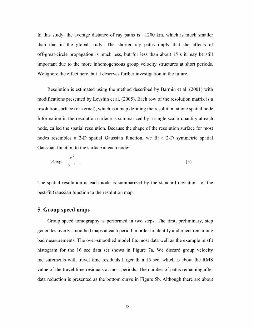
In this study, the average distance of ray paths is ~1200 km, which is much smaller

than that in the global study. The shorter ray paths imply that the effects of

off-great-circle propagation is much less, but for less than about 15 s it may be still

important due to the more inhomogeneous group velocity structures at short periods.

We ignore the effect here, but it deserves further investigation in the future.

Resolution is estimated using the method described by Barmin et al. (2001) with

modifications presented by Levshin et al. (2005). Each row of the resolution matrix is a

resolution surface (or kernel), which is a map defining the resolution at one spatial node.

Information in the resolution surface is summarized by a single scalar quantity at each

node, called the spatial resolution. Because the shape of the resolution surface for most

nodes resembles a 2-D spatial Gaussian function, we fit a 2-D symmetric spatial

Gaussian function to the surface at each node:

2

2

2exp

rA . (5)

The spatial resolution at each node is summarized by the standard deviation of the

best-fit Gaussian function to the resolution map.

5. Group speed maps

Group speed tomography is performed in two steps. The first, preliminary, step

generates overly smoothed maps at each period in order to identify and reject remaining

bad measurements. The over-smoothed model fits most data well as the example misfit

histogram for the 16 sec data set shows in Figure 7a. We discard group velocity

measurements with travel time residuals larger than 15 sec, which is about the RMS

value of the travel time residuals at most periods. The number of paths remaining after

data reduction is presented as the bottom curve in Figure 5b. Although there are about

15

7800 inter-station paths, after data rejection is completed, only about 20%

measurements remain.

The second step of tomography is the construction of the final maps. Maps are

constructed on a 1o x 1o grid across Europe and are defined relative to the reference

maps computed from the 3-D model of Shapiro and Ritzwoller (2002). In an important

sense, the reference maps already have a priori information imposed on crustal

structure. The 3-D model itself was constructed as a perturbation to a starting model

that included information about sediments and crustal thicknesses. For this reason, we

choose to seek only smooth perturbations to the reference maps.

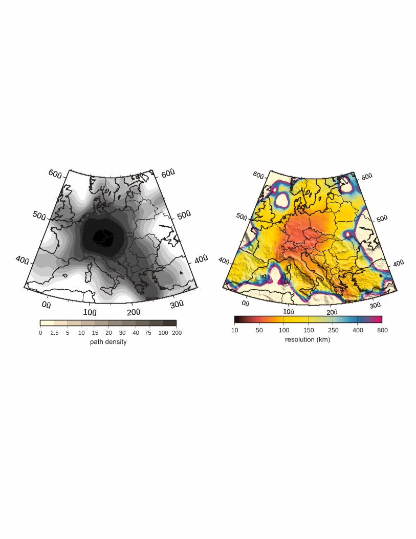
Examples of path density and resolution are shown in Figure 8 for the 16 sec

measurements. Results are similar from 10 sec to 50 sec period, although there is a

reduction in path density and resolution with increasing period due to the decrease in

the number of measurements at long periods, which is caused by the reduction in SNR

above 20 sec period. The resolution of surface wave tomography depends primarily on

path density and the azimuthal distribution of paths. The azimuthal distribution of paths

is good in the center of the study region as demonstrated by Figure 3, but deteriorates

near the boundaries. Path density is highest in the center of Europe and also gradually

degrades toward the edge of the study region. As Figure 8 indicates, average resolution

is estimated to be about 100 km in the center of the study region in Europe, and

degrades toward the periphery of the map where station coverage is minimal.

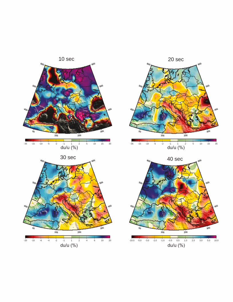
The results of group velocity tomography at 10, 16, 20, 30, 35, and 40 sec periods

are shown in Figures 9, 10a, and 11a. In the inversion, reference group velocity maps

predicted from the global 3-D shear velocity model of Shapiro and Ritzwoller (2002)

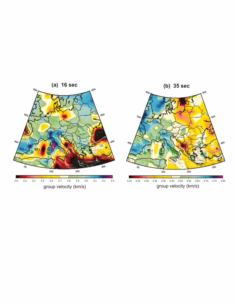
are used as starting models. Examples of the reference maps are shown in Figure 12 at

16 sec and 35 sec period. Figures 10b and 11b illustrate that the perturbations

introduced during tomography are smooth and occur only in regions where path

coverage is high, predominantly in the center of the region of study. In most of the

16

Mediterranean Sea, the Atlantic Ocean, North Africa, the Iberian Peninsula, and far

eastern Europe, the perturbations are small and the estimated maps are very similar to

the reference maps. The features of the maps are observed to vary gradually with period

due to the overlapping depth ranges of Rayleigh wave depth-sensitivity. Many of the

observed anomalies are correlated with known geological units, which is discussed

further in section 6.

Figure 13a shows the improvement in fit to the measured dispersion curves

achieved by the resulting group velocity maps, expressed as the variance reduction

relative to the predicted group velocity maps. In addition, variance reduction relative to

the average across each map is shown. Variance reductions relative to predicted group

velocity (solid line) are larger at short periods (< 25 sec) and smaller at long periods

(>35 sec) than relative to the observed average (dashed line). Variance reductions are

highest at short periods and gradually decrease with period. The observed trend of

variance reductions results from the group speed anomalies bejing largest at short

periods and also because the 3-D model is more reliable for the longer periods. In

particular, Figure 10b illustrates that below about 20 sec period the average of the

reference model is too high. Only periods above about 20 sec went into the construction

of the 3-D model of Shapiro and Ritzwoller (2002). The RMS group velocity and travel

time misfits after tomography are also shown in Figures 13b and 13c. Travel time

misfit of the final data set is ~5 - 6 sec and is nearly independent of period. Contrast

this with the mean uncertainty that trends from ~2 sec to 7 sec shown in Figure 5e.

Most of the misfit at long periods, therefore, is probably due to measurement error. At

short periods, however, about half of the misfit has another cause, perhaps being due to

unspecified structures such as azimuthal anisotropy or smaller scale structures.

6. Discussion

The principal purpose of this paper is to assess the reliability of ambient noise

17

tomography applied to large regions, such as Europe, across a broad frequency band that

extends from short to intermediate periods. We base our assessment on several lines of

evidence: (1) the repeatability of the measurements, (2) the coherence of the

measurements with one another, and (3) the agreement of the resulting group speed maps

with known geological structures. The first two of these criteria have already been

invoked as part of the data selection procedure.

First, the repeatability of the measurements, particularly as they change with the

variable ambient noise conditions in different seasons, is discussed above and is the basis

for the estimates of measurement uncertainties. As discussed in section 5, a measurement

is retained only if it is shown to be robust over multiple seasons. Not all measurements

satisfy this criterion, but many do, as Figure 5b illustrates. This is the foundation for

much of our confidence in the ambient noise dispersion measurements.

Second, the �coherence� of the measurements relates to the mutual agreement of

measurements that cross the same region. This can be determined from the ability to fit

the data with smooth tomographic maps, particularly as that fit compares to that achieved

with earthquake data. Figure 7 plots example histograms of tomographic misfit from

over-smooth maps using ambient noise and earthquake data in Europe measured at CU-B.

The ambient noise data are fit better, partially due to the fact that earthquake data possess

sensitivity to uncertainties in source characteristics. Figure 14 summarizes the standard

deviation of tomographic misfit for both earthquake and ambient noise data across

Europe using the over-smooth maps. These results are taken prior to the last stage in data

rejection; the rejection due to tomographic misfit. This is in contrast to Figure 13c, which

is misfit after data rejection is completed. Figure 13c, therefore, has a lower misfit level.

As periods reduce below 30 sec in Figure 14, relative misfit of ambient noise improves,

particularly below about 15 sec period. We take this as evidence that short-period

dispersion measurements (<20 sec) obtained from ambient noise typically are preferable

to earthquake derived measurements.

18

The final criterion to assess the credibility of the estimated maps is agreement with

known geological structures. Although the best test may be to interpret a 3-D model

constructed from the group speed maps, to address the question more simply one can

exploit how surface waves at different periods are sensitive to Earth structure over

different depth ranges. The depth of maximum sensitivity is about one-third of a

wavelength. At the short-period end of this study (10-20 sec), group velocities are

dominantly sensitive to shear velocities in the upper crust. Because the seismic velocities

of sediments are very low, short-period low velocity anomalies are a good indicator of

sedimentary basins. At the intermediate periods of this study (25-35 sec), Rayleigh waves

are primarily sensitive to crustal thickness and the shear velocities in the lower crust and

uppermost mantle. Due to the large velocity contrasts across the Moho, the group

velocities in this band should vary approximately inversely with crustal thickness, with

high velocities in regions with a thin crust and low velocities regions with a thick crust.

To aid assessment, Figure 15 presents a map of sediment thickness from CRUST1.0,

which Laske and Masters digitized across most of Europe from the EXXON Tectonic

Map of the World (Laske and Masters, 1997), and a map of crustal thickness taken from

CRUST2.0 (Bassin, et al., 2000). We identify the names of several geological units on

these maps, mainly sedimentary basins and mountain ranges.

Comparison of the estimated group speed maps with known geological structures is

the thorniest of the assessment tests, both because understanding of known structures is

imperfect but more pointedly because a priori information has already been imparted to

the reference maps (derived from the 3-D model of Shapiro and Ritzwoller, 2002)) that

form the basis for tomography. In fact, the reference model does not strongly affect the

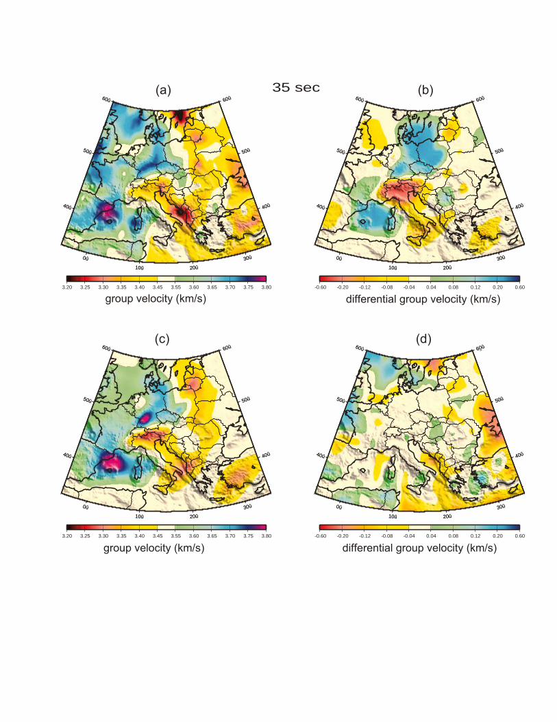
estimated group speed maps in areas of high data coverage. To demonstrate this, Figures

10c and 11c present maps constructed with no input reference model. Comparison with

Figures 10a and 11a establishes the point � in regions of high data coverage an estimated

map can be compared with a priori knowledge without worry of contamination by

19

information contained in the reference map. Figures 10d and 11d also show explicitly that

the reference model imposes little constraint on the estimated map in areas of high data

coverage.

The 10 sec and 16 sec group speed maps in Figures 9 and 10 exhibit low velocity

anomalies associated with most of the known sedimentary basins across Europe. In

regions of high data coverage, low-velocity anomalies are observed in the North Sea

Basin, the Silesian Basin (North Germany, Poland), the Pannonian Basin (Hungary,

Slovakia), the Po Basin (North Italy), the Rhone Basin (Southern France), and the

Adriatic Sea. Not surprisingly, many of these features already exist in the reference map.

Because there is little resolution in the Mediterranean and Black Seas, as Figure 8 shows,

the basins there are imposed by the reference model. The new features recovered from

ambient noise tomography below 20 sec period are (1) a general reduction of group

speeds in the center of the region of study, (2) generation of much more pronounced low

velocity anomalies associated with the Po and Pannonian Basins, and (3) increase in

group speeds directly north of the Hellenic Arc. In particular, the low velocity anomaly

observed in the Pannonian Basin is stronger than expected from the Exxon sediment

maps, which estimates the sediments to be about 2 km thick. A recent study by Grad et al.

(2006) includes a 2-D tomographic model, constructed from a refraction profile running

from the East European craton to the Pannonian Basin. In their model, the sediments of

the Pannonian Basin extend to a depth of ~5 km, which is more consistent with our

observed 5-10% lower group velocities in this region.

At intermediate periods (25 to 40 sec), group velocities become increasingly

sensitive to crustal thicknesses. The estimated maps exhibit low-velocity anomalies

associated with the Alps, the Carpathians and the mountains in the Balkan region. The

low velocity anomalies are probably caused by deeper crustal roots beneath mountain

regions which occur due to isostatic compensation. The general reduction in Rayleigh

wave velocity in the eastern part of the 30 - 40 sec maps in Figures 9 and 11 is probably

20

related to the general thickening of the crust toward the east European craton, where the

crust is about 45 km thick (Grad et al., 2006).

More detailed interpretation of the observed anomalies is beyond the scope of this

work, and awaits complementary research, which will include inversion for the Vs

structure of the crust and upper mantle in Europe. The group velocity maps of our study,

particularly at periods below ~20 sec, provide unique constraints on crustal thickness and

shear wave velocities in the crust and uppermost mantle.

7. Conclusions

In this study, we use ambient noise data recorded at 125 broad-band seismic stations

available from the Global Seismic Network (GSN) and the Orfeus Virtual European

Broad-band seismic Network (VEBSN). Cross-correlations are computed in a broad

period band from 5 sec to 150 sec in daily segments with a duration of one-year. Rayleigh

wave group velocities for station-pairs are measured from one-year stacks of daily

cross-correlations using a phase-match filtering frequency-time analysis procedure.

Uncertainties of the group velocities are estimated based on seasonal variations of the

dispersion curves using three-month time-series. An automated data selection procedure

is applied to all dispersion measurements using signal-to-noise ratio and seasonal

repeatability as selection criteria. About 20% of all station-station cross-correlations are

retained for surface wave tomography after data rejection. All measurements have

uncertainty estimates that derive from observations of seasonal variability. The data set

would benefit from time-series of 2 or more years, which would allow more uncertainties

to be measured and, therefore, more measurements to pass the selection criterion.

Group velocity maps at periods from 10 sec to 50 sec are obtained using ambient

noise tomography. These maps provide a significant improvement in the understanding of

surface wave dispersion in Europe, particularly at periods below about 20 sec. This study

has a denser and more uniform data coverage and demonstrates higher resolution than

21

pervious studies which have relied on traditional earthquake-based surface wave

tomography. Estimated resolution is ~100 km at 10 sec period, but degrades slowly with

period above above 25 sec. Tomographic misfit of group speeds measured from ambient

noise shows a significant improvement over earthquake based measurements below 30

sec period, particularly below 15 sec. The group velocity maps agree quantitatively with

known geologic features, such as sedimentary basins and the lateral variation of crustal

thickness. Observations at short periods (10 - 20 sec) provide entirely new constraints on

sediment thickness, crustal thickness, and the shear velocity structure of crust.

In summary, this study demonstrates that surface wave tomography based on

cross-correlations of long time-series of ambient noise data can be achieved over a broad

period band on a nearly continental scale and yield higher resolution and more reliable

group velocity maps than based on traditional earthquake-based measurements.

Acknowledgments

All of the data used in this research were downloaded from the continuous ftp database of

the Orfeus (Observatories and Research Facilities for European Seismology) Data Center

and from the IRIS Data Management Center. In particular, the authors are deeply grateful

to the data contributors to the Virtual European Broadband Seismic Network (VEBSN), a

partnership of more than 30 local, regional and global arrays and networks. The list of

contributors is located at http://www.orfeus-eu.org/meredian/vebsn-contributors.htm.

Comments from two anonymous reviewers are appreciated. This research was supported

by a contract from the US Department of Energy, DE-FC52-2005NA26607.

22

References

Barmin, M.P., Ritzwoller, M.H., & Levshin, A.L., 2001. A fast and reliable method for

surface wave tomography, Pure Appl. Geophys., 158, 1351 - 1375.

Bassin, C., Laske, G., & Masters, G., 2000. The current limits of resolution for surface

wave tomography in North America, EOS Trans AGU, 81, F897.

Bensen, G.D., Ritzwoller, M.H., Barmin, M.P., Levshin, A.L., Lin, F., Moschetti, M.P.,

Shapiro, N.M., & Yang, Y., 2006. Processing seismic ambient noise data to obtain

reliable broad-band surface wave dispersion measurements, submitted to Geophys. J.

Int.

Cho, K.H., Hermann, R.B., Ammon, C.J., & Lee, K., 2006. Imaging the upper crust of

the Korean Peninsula by surface-wave tomography, Bull. Seism. Soc, Amer.,submitted.

Campillo M., & Paul, A., 2003. Long-range correlations in the diffuse seismic coda,

Science, 299,547-549.

Clevede, E., Megnin, C., Romanowicz, B. & Lognonne, P., 2000. Seismic waveform

modeling and surface wave tomography in a three-dimensional Earth: asymptotic and

non-asymptotic approaches, Phys. Earth Planet. Int., 119,37-56.

Derode, A., Larose, E., Tanter, M., de Rosny, J., Tourim, A., Campillo, M., & Fink, M.,

2003. Recovering the Green�s function from field-field correlations in an open

scattering medium, J. Acoust. Soc. Am., 113,2973-2976.

Grad, M., Guterch, A., Keller, G. R., Janik, T., Heged s, E., Vozár, J., l czka, A., Tiira,

T., & Yliniemi, J., 2006. Lithospheric structure beneath trans-Carpathian transect from

23

Precambrian platform to Pannonian basin: CELEBRATION 2000 seismic profile

CEL05, J. Geophys. Res., 111, B03301, doi:10.1029/2005JB003647.

Larose, E., Derode, A., Campillo, M., & Fink, M., 2004. Imaging from one-bit

correlations of wideband diffuse wavefields, J. Appl. Phys., 95, 8393-8399.

Larose, E., Derode, A., Corennec, D., Margerin, L., & Campillo, M., 2005. Passive

retrieval of Rayleigh waves in disoredered elastic media, Phys. Rev. E., 72, 046607,

doi:10.113/PhysRevE.72.046607.

Laske, G.., & Masters, G.., 1997. A Global Digital Map of Sediment Thickness, EOS

Trans. AGU, 78, F483.

Levshin, A.L. & Ritzwoller, M.H., 2001. Automated detection, extraction, and

measurement of regional surface waves, Pure Appl. Geophys., 158, 1531-1545.

Levshin, A.L., Barmin, M.P., Ritzwoller, M.H., & Trampert, J., 2005. Minor-arc and

major-arc global surface wave diffraction tomography, Phys. Earth Planet. Ints., 149,

205-223.

Levshin, A.L., Schweitzer, J., Weidle, C., Shapiro, N.M., & Ritzwoller, M.H., 2006.

Surface wave tomography of the Barents Sea and surrounding regions, Geophys. J. Int.,

in press,

Lin, F., Ritzwoller, M. H., & Shapiro, N. M., 2006. Is ambient noise tomography across

ocean basins possible?, Geophys. Res. Lett., 33, L14304, doi:10.1029/2006GL026610.

Lomax, A., & Snieder, R., 1995. The contrast in the upper mantle shear-wave velocity

between the East European Platform and tectonic Europe obtained with genetic

algorithm inversion of Rayleigh-wave group velocity dispersion, Geophys. J. Int.,

24

123,169-182.

Marquering, H., & Snieder, R., 1996. Shear-wave velocity structure beneath Europe, the

northeastern Atlantic western Asia from wavefrom inversions including surface-wave

mode coupling, Geophys. J. Int., 127, 283-304.

Maupin, V., & Cara, M., 1992. Love-Rayleigh wave incompatibility and possible deep

upper mantle anisotropy in the Iberian peninsula, Pure Appl. Geophys., 138(3),

429-444.

Moschetti, M. P., Ritzwoller, M. H., & Shapiro, N. M., 2005. California Surface Wave

Tomography from Ambient Seismic Noise: Tracking the Progress of the USArray

Transportable Network, Eos Trans. AGU, 86(52), Fall Meet. Suppl., Abstract

S31A-0276

Mueller, S., & Sprecher, C., 1978. Upper mantle structure along a profile through the

eastern Alps from Rayleigh wave dispersion, in Alps, Apennines, Hellenides, edited by

H. Closs, Int. Geodyn. Comm. Sci. Rep., 38, 40-44.

Nolet, G., 1977. The upper mantle under western Europe inferred form the dispersion of

Rayleigh wave modes, J. Geophys., 43, 265-276.

Panza, G.F., Mueller, S., & Calcagnile, G., 1980. The gross features of the

lithosphere-asthenosphere system in Europe from seismic surface waves and body

waves, Pure Appl. Geophys., 118, 1209-1213.

Papazachos, B.C., 1969. Phase velocities of Rayleigh waves in Southeastern Europe

and Eastern Mediterranean Sea, Pure Appl. Geophys., 75, 47-55.

Pontevivo, A., & Panza, G. F., 2002. Group velocity tomography and regionalization in

25

Italy and bordering areas, Phys. Earth Planet. Inter., 134, 1-15.

Pasyanos, M.E., 2005. A variable resolution surface wave dispersion study of Eurasia,

North Africa, and surrounding regions, J. Geophys. Res., 110, B12301, doi:

10.1029/2005JB003749.

Pasyanos, M. E. & Walter, W. R., 2002. Crust and upper-mantle structure of North Africa,

Europe and the Middle East from inversion of surface waves, Geophys. J. Int.,

149,463-481.

Patton, H., 1980. Crustal and upper mantle structure of the Eurasian continent from the

phase velocity and of surface wave, Rev. Geophys., 18,605-625. Q

Paul, A., Campillo, M., Margerin, L., Larose, E., & Derode, A., 2005. Empirical synthesis

of time-asymmetrical Green functions from the correlation of coda waves, J. Geophys.

Res., 110, B08302, doi:10.1029/2004JB003521.

Pedersen, H. A., Campillo, M., & Balling, N., 1994. Changes in the lithospheric structure

across the Sorgenfrei-Tornquist Zone inferred from dispersion of Rayleigh waves,

Earth Planet. Sci. Lett., 128,37-46.

Ritzwoller, M. H. & Levshin, A. L., 1998. Eurasian surface wave tomography: group

velocities, J. Geophys. Res., 103, 4839-4878.

Ritzwoller, M. H., Shapiro, N. M., Barmin, M. P., & Levshin, A.L., 2002. Global surface

wave diffraction tomography, J. Geophys. Res., 107, B12, 10.1029/2002JB001777.

Roux, P., Sabra, K.G., Gerstoft, P., Kuperman, W.A., & Fehler, M.C., 2005. P-waves from

cross-correlation of seismic noise, Geophys. Res. Lett., 32, L19393,

doi:10.1029/2005GL023803.

26

Sabra, K., Gerstoft, G., P., Roux, P., Kuperman, W. A., & Fehler, M. C., 2005a.

Extracting time-domain Green�s function estimates from ambient seismic noise,

Geophys. Res. Lett., 32, L03310, doi:10.1029/2004GL021862.

Sabra, K. Gerstoft, G., Roux, P., Kuperman, W. A., & Fehler, M. C., 2005b. Surface

wave tomography from microseism in southern California, Geophys. Res. Lett., 32,

L14311, doi:10.1029/2005GL023155.

Shapiro, N.M. & Campillo, M., 2004. Emergence of broadband Rayleigh waves from

correlations of the ambient seismic noise, Geophys. Res. Lett., 31, L07614,

doi:10.1029/2004GL019491.

Shapiro, N.M. & Ritzwoller, M.H.,2002. Monte-Carlo inversion for a global shear

velocity model of the crust and upper mantle, Geophys. J. Int., 151, 88-105.

Shapiro, N.M. Campillo, M., Stehly, L., & Ritzwoller, M.H., 2005. High resolution

surface wave tomography from ambient seismic noise, Science, 307, 1615-1618.

Sieminski, A., Leveque, J.-J., & Debayle, E., 2004. Can finite-frequency effects be

accounted for in ray theory surface wave tomography?, Geophys. Res. Lett., 31,

L24614, doi:10.1029/2004GL021402.

Snieder, R., 1988. Large-scale waveform inversions of surface saves for lateral

heterogeneity, 2, application to surface saves in Europe and the Mediterranean, J.

Geophys. Res., 93, 12067-12080.

Snieder, R., 2004. Extracting the Green's function from the correlation of coda waves: A

derivation based on stationary phase, Phys. rev. E, 69, 046610.

Spetzler, J., Trampert, J. & Snieder, R., 2002. The effects of scattering in surface wave

27

tomography, Geophys. J. Int., 149,755-767.

Stange, S., & Friederich, W., 1993. Surface wave dispersion and upper mantle structure

beneath southern Germany from joined inversion of network recorded teleseismic

events, Geophys. Res. Lett., 20, 2375-2378.

Vaccari, F., & Panza, G. F., 1993. Vp/Vs estimation in southwestern Europe from P-wave

tomography and surface wave tomography analysis, Phys. Earth Planet. Inter., 78,

229-237.

Wapenaar, K., 2004. Retrieving the elastodynamic Green�s function of an arbitrary

inhomogeneous medium by cross correlation, Phys. Rev. Lett., 93, 254301,

doi:10.1103/PhysRevLett.93.254301.

Weaver, R.L. & Lobkis, O. I., 2001a. Ultrasonics without a source: Thermal fluctuation

correlation at MHZ frequencies, Phys. Rev. Lett., 87, paper 134301.

Weaver, R.L. & Lobkis, O.I., 2001b. On the emergence of the Green's function in the

correlations of a diffuse field, J. Acoust. Soc. Am., 110, 3011-3017.

Weaver, R.L. & Lobkis, O.I., 2004. Diffuse fields in open systems and the emergence of

the Green�s function, J. Acoust. Soc. Am., 116, 2731-2734.

Yanovskaya, T.B., Antonova, L.M., & Kozhevnikov, V.M., 2000. Lateral variations of

the upper mantle structure in Eurasia from group velocities of surface waves, Phys.

Earth Planet. Inter., 122, 19-32.

Yao, H., van der Hilst, R.D., & De Hoop, M.V., 2006. Surface-wave array tomography in

SE Tibet from ambient seismic noise and two-station analysis: I - Phase velocity maps,

Geophys. J. Int., 166, 732-744.

28

Yoshizawa, K. & Kennett, B. L. H., 2002. Determination of the influence zone for surface

wave paths, Geophys. J. Int., 149,440-453.

Zhou Y., Dahlen, F.A. & Nolet, G., 2004. 3-D sensitivity kernels for surface-wave

observables, Geophys. J. Int., 158, 142-168.

Figure captions:

Figure 1. Broad-band seismic stations in Europe used in this study, marked by red

triangles.

Figure 2. Example of a 12-month broad-band symmetric-component cross-correlation

between the station-pair IBBN (Ibbenbueren, Germany) and TIRR (Hungary). The red

line shows the great-circle linking the two stations. The broad-band cross-correlation

(right) is filtered into five sub-bands. Note the clear normal dispersion of the Rayleigh

waves, with the longer periods arriving earlier.

Figure 3. Example of a 12-month symmetric-component cross-correlation record-section

centered on the station TUE (Stuetta, Italy) and band-pass filtered from 20 � 50 sec

period. Only cross-correlations with SNR > 7 are shown at right with the corresponding

paths delineated by red lines at left. The diagonal gray line indicates the approximate

arrival time for Rayleigh waves in this band.

Figure 4. Example of dispersion measurement. (Top) One-year symmetric component

cross-correlation obtained between stations IBBN (Ibbenbueren, Germany) and OBN

(Obninsk, Russia), which are separated by 1900 km. (Middle) Raw frequency-time

29

(FTAN) diagram in which the thick line is the raw dispersion measurement. (Bottom)

Cleaned FTAN diagram obtained after applying the phase-matched filter based on the

raw dispersion measurement. The thin line in the Middle and Bottom panels is the

dispersion curve predicted from the global 3-D shear velocity model (Shapiro and

Ritzwoller, 2002). The cleaned waveform is overplotted in the top panel as a dashed line.

Figure 5. (a) Number of measurements versus signal-to-noise ratio from the 12-month

stacked cross-correlations. (b) Number of measurements remaining after several steps in

data reduction. (c) Average path length of the accepted dispersion measurements. (d)

Average group speed uncertainties versus period. (e) Average travel time uncertainties

versus period.

Figure 6. An example of seasonal variability of the dispersion measurements. (Top)

The path considered is between stations HGN (Heijmans Groeve, Netherlands) and PSZ

(Piszkes-teto, Hungary). (Bottom) The red curves are group velocity measurements

obtained on twelve 3-month cross-correlations band-pass filtered from 8 to 50 sec period.

The black line is the prediction from the global 3-D model (Shapiro and Ritzwoller,

2002).

Figure 7. Histograms of misfit for ambient noise data (left) and earthquake data (right) at

16 sec period. Misfit is calculated from the corresponding over-smooth tomographic map

inverted from ambient noise data and earthquake data. Ambient noise data are taken prior

to the stage where measurements are rejected due to large misfit. The standard deviation

is shown at the left top of each diagram.

Figure 8. Path density (left column) and resolution estimates (right column) at 16 sec

period. Path density is defined as the number of rays intersecting a 00 11 (111 km x 111

30

km) square cell. Resolution is presented in units of km, and is defined as the standard

deviation of a 2-D Gaussian fit to the resolution surface at each model node.

Figure 9. Estimated group speed maps at 10, 20, 30, and 40 sec periods. Maps are

presented as a perturbation from the average across the map in percent.

Figure 10. Group speed maps at 16 sec period. (a) Estimated group speed map

determined with a reference map. (b) Difference between the estimated map in (a) and the

reference map presented in Fig. 12a. (c) Estimated group speed map determined without

a reference map. (d) Difference between the two estimated maps in (a) and (c).

Figure 11. Same as Fig. 10, but for 35 sec period. The reference map used is presented in

Fig. 12b.

Figure 12. Reference maps computed from the 3-D model of Shapiro and Ritzwoller

(2002) at (a) 16 sec and (b) 35 sec period.

Figure 13. Various misfit statistics for the estimated group speed maps to the

observations taken after all stages of data rejection are complete. (a) Misfit is presented

as reduction of variance delivered by the estimated maps relative to (solid line) the

predicted group velocity maps from the global 3-D model (Shapiro and Ritzwoller, 2002)

and (dashed line) the average velocity across each map. (b) RMS group velocity misfit

presented versus period. (c) RMS travel time misfit presented versus period.

Figure 14. Standard deviations of data misfit after tomography with an over-smoothed

model, presented as a function of period for ambient noise data (solid line) and

earthquake data (dashed line). In contrast with Figure 13c and similar to Figure 7, the last

31

stage of data rejection has not been applied here.

Figure 15. Maps of sediment thickness (left) and crustal thickness (right). Sediment

thicknesses are taken from CRUST1.0, which Laske and Masters digitized across most of

Europe from the EXXON Tectonic Map of the World. Crustal thicknesses are taken from

CRUST2.0. The locations of geological units discussed in the text are marked

approximately.

32

350û

0û

10û 20û 30û

40û

50û

30û 30û

40û 40û

50û 50û

60û 60û

70û 70û

350û

0û

10û 20û 30û

40û

50û

30û 30û

40û 40û

50û 50û

60û 60û

70û 70û

350û

0û

10û 20û 30û

40û

50û

30û 30û

40û 40û

50û 50û

60û 60û

70û 70û

350û

0û

10û 20û 30û

40û

50û

30û 30û

40û 40û

50û 50û

60û 60û

70û 70û

IBBN

TIRR

time ( 100× sec )

8 to 25 s

20 to 50 s

33 to 67 s

50 to 100 s

70 to 150 s

5 to 150 s

350û

0û10û 20û

30û

40û

30û 30û

40û 40û

50û 50û

60û 60û

350û

0û10û 20û

30û

40û

30û 30û

40û 40û

50û 50û

60û 60û

time ( 100× sec )

dis

tance (

100

km

)×

TUE

no

rma

lize

d v

elo

city

gro

up

ve

loci

ty

( km

/s)

raw F T AN

period ( s )

gro

up

ve

loci

ty

( km

/s)

cleaned F T AN

1.

2.

2.

3.

3.

4.

4.

1.

2.

2.

3.

3.

4.

4.

5

0

5

0

5

0

5

10 20 30 40 50

5

0

5

0

5

0

5

10 20 30 40 50

1.5

2.0

2.5

3.0

3.5

4.0

4.5

10 20 30 40 50

1.5

2.0

2.5

3.0

3.5

4.0

4.5

10 20 30 40 50

400 500 600 700 900 1000-1

-0.8

-0.6

-0.4

-0.2

0

0.2

0.4

0.6

0.8

1

800

time (s )

nu

mb

er

of

me

asu

rem

en

tsp

ath

len

gth

(km

)

velo

city

un

cert

ain

ties

(km

/s)

tra

vel t

ime

un

cert

ain

ties

(s)

0 10 20 30 400

500

1000

10 20 30 40 50500

1000

1500

2000

10 20 30 40 500

0.05

0.1

10 20 30 40 502

4

6

8

s ignal-to-noise ratio

period (s )

period (s ) period (s )

(a)

10 20 30 40 50

1000

2000

3000

4000

nu

mb

er

of

me

asu

rem

en

ts

period (s )

S NR > 7

S T D exists

fitting smooth model

(b)

(c) (d)

(e)

grou

p ve

loci

ty (k

m/s

)

period

3-D model prediction

3-month stacks

2.0

2.5

3.0

3.5

4.0

4.5

10 15

2.0

2.5

3.0

3.5

4.0

4.5

10 15

2.0

2.5

3.0

3.5

4.0

4.5

10 15

2.0

2.5

3.0

3.5

4.0

4.5

10 15

2.0

2.5

3.0

3.5

4.0

4.5

10 15

2.0

2.5

3.0

3.5

4.0

4.5

10 15

2.0

2.5

3.0

3.5

4.0

4.5

10 15

2.0

2.5

3.0

3.5

4.0

4.5

10 15

2.0

2.5

3.0

3.5

4.0

4.5

10 15

2.0

2.5

3.0

3.5

4.0

4.5

10 15

2.0

2.5

3.0

3.5

4.0

4.5

10 15

2.0

2.5

3.0

3.5

4.0

4.5

10 15

2.0

2.5

3.0

3.5

4.0

4.5

10 15

2.0

2.5

3.0

3.5

4.0

4.5

10 15

2.0

2.5

3.0

3.5

4.0

4.5

10 15

2.0

2.5

3.0

3.5

4.0

4.5

10 15

2.0

2.5

3.0

3.5

4.0

4.5

10 15

2.0

2.5

3.0

3.5

4.0

4.5

10 15

2.0

2.5

3.0

3.5

4.0

4.5

10 15

2.0

2.5

3.0

3.5

4.0

4.5

10 15

2.0

2.5

3.0

3.5

4.0

4.5

10 15

2.0

2.5

3.0

3.5

4.0

4.5

10 15

2.0

2.5

3.0

3.5

4.0

4.5

10 15 20 25 30 35 40 45 5020 25 30 35 40 45 5020 25 30 35 40 45 5020 25 30 35 40 45 5020 25 30 35 40 45 5020 25 30 35 40 45 5020 25 30 35 40 45 5020 25 30 35 40 45 5020 25 30 35 40 45 5020 25 30 35 40 45 5020 25 30 35 40 45 5020 25 30 35 40 45 5020 25 30 35 40 45 5020 25 30 35 40 45 5020 25 30 35 40 45 5020 25 30 35 40 45 5020 25 30 35 40 45 5020 25 30 35 40 45 5020 25 30 35 40 45 5020 25 30 35 40 45 5020 25 30 35 40 45 5020 25 30 35 40 45 5020 25 30 35 40 45 50

(s)

350

0

1020 30

40

50

30

40 40

50 50

60 60

350

0

1020 30

40

50

30

40 40

50

60

HGN

PSZ

00 80 60 0 0 0 20 40 60 80 1000

100

200

300

400

500

600

700

misfit to ambient noise measurements: 16 sec

st dev = 12.6 sec

misfit (sec)00 80 60 0 0 0 20 40 60 80 100

0

20

40

60

80

100

120

140

st dev = 22.7 sec

misfit (sec)

misfit to earthquake measurements: 16 sec

10 50 100 150 250 400 8000 2.5 5 10 15 20 30 40 75 100 200

path density resolution (km)

0û10û 20û

30û

40û 40û

50û 50û

60û 60û

0û10û 20û

30û

40û 40û

50û 50û

60û 60û

0û10û 20û

30û

40û 40û

50û 50û

60û 60û

0û10û 20û

30û

40û 40û

50û 50û

60û 60û

0û

10û 20û

30û

40û 40û

50û 50û

60û 60û

0û

10û 20û

30û

40û 40û

50û 50û

60û 60û

-35 -15 -10 -5 -2 -1 1 2 5 10 15 35

0û

10û 20û

30û

40û 40û

50û 50û

60û 60û

0û

10û 20û

30û

40û 40û

50û 50û

60û 60û

-35 -15 -10 -5 -2 -1 1 2 5 10 15 35

0û

10û 20û

30û

40û 40û

50û 50û

60û 60û

0û

10û 20û

30û

40û 40û

50û 50û

60û 60û

-20 -10 -6 -4 -2 -1 1 2 4 6 10 20

0û

10û 20û

30û

40û 40û

50û 50û

60û 60û

0û

10û 20û

30û

40û 40û

50û 50û

60û 60û

-10.0 -5.0 -3.0 -2.0 -1.0 -0.5 0.5 1.0 2.0 3.0 5.0 10.0

10 sec 20 sec

30 sec 40 sec

du/u (%)du/u (%)

du/u (%)du/u (%)

group velocity (km/s)

group velocity (km/s) differential group velocity (km/s)

differential group velocity (km/s)

(a) (b)

(c) (d)

0û

10û 20û

30û

40û 40û

50û 50û

60û 60û

0û

10û 20û

30û

40û 40û

50û 50û

60û 60û

2.0 2.3 2.4 2.5 2.6 2.7 2.8 2.9 3.0 3.1 3.2 3.3

0û

10û 20û

30û

40û 40û

50û 50û

60û 60û

0û

10û 20û

30û

40û 40û

50û 50û

60û 60û

-0.70 -0.45 -0.35 -0.25 -0.15 -0.05 0.05 0.15 0.25 0.35 0.45 0.70

16 sec

0û

10û 20û

30û

40û 40û

50û 50û

60û 60û

0û

10û 20û

30û

40û 40û

50û 50û

60û 60û

-0.70 -0.45 -0.35 -0.25 -0.15 -0.05 0.05 0.15 0.25 0.35 0.45 0.70

0û

10û 20û

30û

40û 40û

50û 50û

60û 60û

0û

10û 20û

30û

40û 40û

50û 50û

60û 60û

2.0 2.3 2.4 2.5 2.6 2.7 2.8 2.9 3.0 3.1 3.2 3.3

group velocity (km/s)

group velocity (km/s) differential group velocity (km/s)

differential group velocity (km/s)

(a) (b)

(c) (d)

0û

10û 20û

30û

40û 40û

50û 50û

60û 60û

0û

10û 20û

30û

40û 40û

50û 50û

60û 60û

3.20 3.25 3.30 3.35 3.40 3.45 3.55 3.60 3.65 3.70 3.75 3.80

0û

10û 20û

30û

40û 40û

50û 50û

60û 60û

0û

10û 20û

30û

40û 40û

50û 50û

60û 60û

-0.60 -0.20 -0.12 -0.08 -0.04 0.04 0.08 0.12 0.20 0.60

35 sec

0û

10û 20û

30û

40û 40û

50û 50û

60û 60û

0û

10û 20û

30û

40û 40û

50û 50û

60û 60û

3.20 3.25 3.30 3.35 3.40 3.45 3.55 3.60 3.65 3.70 3.75 3.80

0û

10û 20û

30û

40û 40û

50û 50û

60û 60û

0û

10û 20û

30û

40û 40û

50û 50û

60û 60û

-0.60 -0.20 -0.12 -0.08 -0.04 0.04 0.08 0.12 0.20 0.60

(a) 16 sec (b) 35 sec

group velocity (km/s) group velocity (km/s)

0û

10û 20û

30û

40û 40û

50û 50û

60û 60û

0û

10û 20û

30û

40û 40û

50û 50û

60û 60û

3.20 3.25 3.30 3.35 3.40 3.45 3.55 3.60 3.65 3.70 3.75 3.80

0û

10û 20û

30û

40û 40û

50û 50û

60û 60û

0û

10û 20û

30û

40û 40û

50û 50û

60û 60û

2.0 2.3 2.4 2.5 2.6 2.7 2.8 2.9 3.0 3.1 3.2 3.3

10 20 30 40 500

20

40

60

80

vari

an

ce r

ed

uct

ion

(%

)

10 20 30 40 500.04

0.06

0.08

0.1

0.12

RM

S g

rou

p v

elo

city

mis

fit (

km/s

)

10 20 30 40 502

3

4

5

6

7

8

period (s )

RM

S t

rave

l tim

e m

isfit

(s)

(a)

(b)

(c)

0 10 20 30 40 500

10

20

30

40

50

earthquakes

ambient noise

period (sec)

mis

fit (

st d

ev

in s

ec)

12 15 18 21 24 27 30 33 36 39 42 45

0

10 20

30

40 40

50 50

60 60

0

10 20

30

40 40

50 50

60 60

crustal thickness

0 1 2 3 4 5 6 7 8 9 10

sediment thickness

10 20

50

60 60

10 20

50

60 60

40

1112

138

10

2

sediment thickness (km) crustal thickness (km)

1. North Sea 2. Black Sea 3. Silesian Basin 4. Pannonian Basin

5. Po Basin 6. Rhone Basin 7. Paris Basin 8. Adriatic Sea

9. W. Mediterranean 10. E. Mediterranean 11. Alps 12. Carpathians

13. Balkans