Daniel L. Thornton and Piyu Vise

Daniel L. Thornton is an assistant vice president at the FederalReserve Bank of St Louis. Piyu Yue, a research associate atthe lC2 Institute, University of Texas at Austin, was a visitingscholar at the Federa/ Reserve Bank of St. Louis when thisartic/e was written. Lynn Dietrich and Kevin White providedresearch assistance.

An Extended Series of DivisiaMonetary Aggregates

rj-iI HE CONVENTION IN monetary economics

has been to create monetary aggregates bysimply adding together the dollar amounts ofthe various financial assets included in them.This is the simple-sum method of aggregation.This procedure has been criticized because suchmonetary aggregates are essentially indexes thatweight each component financial asset equally,a practice that is economically meaningful onlyunder special circumstances.

A number of alternative indexes of monetaryaggregates have been developed recently. Themost well known are the Divisia monetaryaggregates developed by Barnett (1980). Thisarticle reviews the theoretical basis for monetaryaggregation and presents series of Divisia

monetary aggregates for an extended sampleperiod. The behavior of the simple-sum aggregatesand their Divisia counterparts are comparedover this period.

ji.iEI..)R~E.’F.K.h~rt1. ~Bz%S.iS44)14NIO.NE’F/1t~V.AG4.IL.EG~~tF1()iN~

Simple-sum aggregation stemmed directly fromthe classical economists’ notion that the essentialfunction of money is to facilitate transactions,that is, to serve as a medium of exchange. Assetsthat served as media of exchange were consid-ered money and those that did not, were not.By this definition only two assets, currency anddemand deposits, were considered money. Bothassets were non-interest bearing, and individuals

1The discussion in this section is based on consumerdemand theory. This may not be a serious limitation. Forexample, Feenstra (1986) has shown that money in theutility function is equivalent to other approaches. Theseapproaches assume, however, that all of the costs andbenefits of money are internalized, and it is commonlybelieved that there are externalities to the use of money inexchange (see Laidler 119901).

36

were free to alter the composition of theirmoney holdings between currency and demanddeposits at a fixed one-to-one ratio. Consequentlythe monetary value of transactions was exactlyequal to the sum of the two monies.2 Simple-sum aggregation was a natural extension ofboth restricting the definition of money to non-interest-bearing medium-of-exchange assets andof the fixed unitary exchange rate between thetwo alternative monies.~

In consumer demand theory, simple-sumaggregation is tantamount to treating currencyand demand deposits as if they are perfect sub-stitutes. Currency and demand deposits, however,are not equally useful for all transactions, sothis assumption was clearly inappropriate. But,simple-sum aggregation of those two monetaryassets was still appropriate because the assetswere non-interest bearing and exchanged at afixed one-to-one ratio. Consequently individualswould allocate their portfolio of money betweenthe two assets until they equalized the marginalutilities of the last dollar held of each. Underthese conditions, simple-sum aggregation is ap-propriate if it is also assumed that each agentis holding his equilibrium portfolio.

The recognition that non-interest-bearingdemand deposits may have paid an implicitinterest weakened the theoretical justification forsimple-sum aggregation. A more serious blowto simple-sum aggregation, however, was dealtby a shift in monetary theory to emphasizingthe store-of-value function of money.4 That an

asset could not be used directly to facilitatetransactions was no longer a sufficient conditionfor excluding it from the definition of money.Instead, the asset approach to money emphasizedmoney’s role as a temporary abode of purchasingpower that bridges the gap between the sale ofone item and the purchase of another. Currencyand checking accounts are money because theyare both media of exchange and temporaryabodes of purchasing power. Non-medium ofexchange assets are superior to currency andnon-interest-bearing checking accounts asstores of value because they earn explicit interest.This superiority typically increases with thelength of time between the sale of one itemand subsequent purchase of another becausethe cost of getting into and out of such assetsand the medium of exchange assets is thoughtto be small and not proportional to the size ofthe transaction.

This shift in emphasis in monetary theorydramatically expanded the number of assetsthat were considered money and the numberof alternative monetary aggregates pro1iferated.~Nonetheless, the method of aggregation remainedthe same—simple-sum aggregation.

As more financial assets came to be consideredmoney, it became increasingly clear that it wasinappropriate to treat these assets as perfectsubstitutes. Some financial assets have more“moneyness” than others, and hence they shouldreceive larger weights. In what appears to bethe first attempt at constructing a theoretically

2This need not be true for the economy as a whole whenmeasured over a sufficiently long time interval. In this casethe amount of each form of money multiplied by its turnovervelocity will equal total expenditures. This is the basis forthe velocity of the demand for money. Fisher (1911) explicitlyrecognized that turnover velocities of currency and checkabledeposits would likely be different. He circumvented thisproblem by assuming that there was an optimal currency-to-deposit ratio that would be a function of economic variables.Given these variables, the demand for the two alternativemonetary assets was taken to be strictly proportional. More-over, because individuals were free to adjust their moneyholdings between currency and checkable deposits quicklyand at low cost, Fisher argued that the actual ratio woulddeviate from the desired ratio for only short periods. Forsome recent evidence that the actual currency-to-depositratio might be determined by the policy actions of theFederal Reserve, see Garfinkel and Thornton (1991). Thepossibility that currency and checkable deposits have differentturnover velocities is the basis for Spindt’s (1985) weightedmonetary aggregate, MO.

3There is an issue of whether the fixed ratio was endogenous,from either the perspective of supply or demand, or theresult of arbitrary legal restrictions. From the demand side,this would require that these assets be perfect substitutesfor all transactions. From the supply side, Pesek and Saving

(1967) argued that the one-to-one exchange rate was anatural outcome of competitive pressures in the bankingindustry. Whether the fixed one-to-one ratio is the endogenousoutcome of a free market economy or is simply due to legalrestrictions remains controversial.

Of course today some checkable deposits earn explicitinterest. Consequently such deposits are a better store ofwealth than currency. They are also a preferable medium ofexchange for some, but not all, transactions.

4There has been a difference of opinion about the degree ofemphasis that should be placed on the asset and transac-tions motives for holding money. Indeed, Laidler (1990,pp. 105—6) has noted that”.., the most extraordinarydevelopment in monetary theory over the past fifty years isthe way in which money’s means-of-exchange and unit-of-account roles have vanished from what is widely regardedas the mainstream of monetary theory.”

Broaching the medium-of-exchange line of demarcationbetween money and non-money assets also gave rise to anextensive literature on the empirical definition of money. Fora critique of this literature and the idea of distinguishingbetween monetary and non-monetary assets based on theconcept of the temporary abode of purchasing power, seeMason (1976).

~Atone point the Federal Reserve published data on fivealternative monetary aggregates.

preferable alternative to the simple-sum monetaryaggregate, Chetty (1969) added various savings-type deposits, weighted by estimates of thedegree of substitution between them and thepure medium of exchange assets, to currencyand demand deposits. Larger weights were givento assets with a higher estimated degree ofsubstitution.°

Divisia aggregation, which also relies onconsumer demand theory and the theory ofeconomic aggregation, treats monetary assets asconsumer durables such as cars, televisions andhouses. They are held for the flow of utility-generating monetary services they provide. Intheory, the service flow is given by the utilitylevel. Consequently the marginal service flow ofa monetary asset is its marginal utility. Inequilibrium, the marginal service flow of amonetary asset is proportional to its rental rate,so the change in the value of a monetary asset’sservice flow per dollar of the asset held can beapproximated by its user cost. The marginalmonetary services of the components of Divisiaaggregates are likewise proxied by the usercosts of the component assets. The user cost ofeach component is proportional to the interestincome foregone by holding it rather than apure store-of-wealth asset—an asset that yields ahigh rate of return but provides no monetaryservices. Currency and non-interest-bearingdemand deposits have the highest user costbecause they earn no explicit interest income.Consequently they get the largest weights in theDivisia measure. On the other hand, pure store-of~wealthassets get zero weights.~

The object of a Divisia measure is to constructan index of the flow of monetary services from

a group of monetary assets, where the monetaryservice flow per dollar of the asset held canvary from asset to asset.8 Applying an appropriateindex number to a group of assets is not sufficient,however, to get a correct measure of the flowof monetary services. The index must also beconstructed from a set of assets that can beaggregated under conditions set by consumerdemand theory. The objective of economicaggregation is to identify a group of goods thatbehave as if they were a single commodity. Anecessary condition for this is block-wise weakseparability. Block-wise weak separability requiresthat consumers’ decisions about goods that areoutside the group do not influence their pre-ferences over the goods in the group whatso-ever.9 If this condition is satisfied, consumersbehave just as though they were allocating theirincomes over a single aggregate measure ofmonetary services and all other commodities tomaximize their utility. l’heir total expenditureon monetary services is subsequently allocatedover the various financial assets that providesuch services.

The Divisia index generates such a monetaryaggregate. Moreover, in continuous time it hasbeen shown to be consistent with any unknownutility function implied by the data. In discretetime the Divisia index is in the class of superlativeindex numbers. Simple-sum indexes, on theother hand, do not have this desirable property.Thus they have no basis in either consumerdemand theory or aggregation theory.10

In principle, all financial assets other thanpure store-of-wealth assets provide some monetaryservices. Which assets can be combined into ameaningful monetary aggregate is an empirical

6Chetty’s work was motivated by the Gurley/Shaw hypothesisand the general lack of agreement in the empirical findingsof Feige (1964) and others about the degree of substitutabilitybetween money and near-money assets. Gurley and Shaw(1960) suggested that the effectiveness of monetary policywas limited because of the high degree of substitutabilitybetween money (currency and demand deposits) and near-money (various bank and nonbank savings-type accounts)assets. Subsequent research has tended to support Feige’sfinding of a relatively low degree of substitutability betweentransactions media and liquid, non-medium-of-exchangeassets. See Fisher (1989) for a survey ot much of this literature.

7There does not appear to be agreement about what consti-tutes the best proxy measure for the theoretical pure store-of-wealth asset. Barnett, Fisher and Serletis (1992, p. 2,093)state the following, ‘The benchmark asset is specificallyassumed to provide no liquidity or other monetary servicesand is held solely to transfer wealth intertemporally. Intheory, R (the benchmark rate) is the maximum expectedholding period yield in the economy. It is usually defined inpractice in such a way that the user costs for the monetary

assets are (always) positive.” Parentheses added. TheBaa bond rate, or the highest rate paid on any of thecomponent assets when the yield curve becomesinverted, has frequently been used to construct Divisiaaggregates.

9See Barnett, Fisher and Serletis (1992) and Yue (1991aand b) for more detailed analyses of issues in monetaryaggregation.

9Technically the marginal rates of substitution between anytwo goods inside the group must be independent of thequantities of the goods consumed that are outside of thegroup.

‘°Fisher(1922) was especially critical of the simple-sumindex in his extensive analysis of index numbers. In parti-cular, Fisher argued that simple-sum aggregates cannotinternalize pure substitution effects associated with relativeprice changes. Thus changes in utility, which should occuronly as a result of the income effect associated withrelative price changes, occur in simple-sum aggregatesbecause of both income and substitution effects.

38

issue because economic theory does not tell uswhich group of assets satisfies the condition ofblock-wise weak separability. Unfortunately, themost widely used test for weak separability isnot powerful.” Consequently, it has been commonsimply to create Divisia indexes under themaintained hypothesis that the assets thatcompose the aggregate satisfy this condition.Thus the issues of the appropriate method ofaggregation and the appropriate aggregate havebeen treated separately.’~

~ tr~1)i.:irszis~

.414r61)F,:4Hi IJEXJ)S

A simple-sum monetary aggregate is a measureof the stock of financial assets that compose it,whereas a Divisia monetary aggregate is ameasure of the flow of monetary services fromthe stocks of financial assets that compose it.13

For this reason alone, the methods of measure-ment are quite different. Simple-sum aggregatesare obtained by simply adding the dollar amountsof the component assets. On the other hand,Divisia monetary aggregates are obtained bymultiplying each component asset’s growth rateby its share weights and adding the products.A component’s share weight depends on theuser costs and the quantities of all componentassets.’4 Specifically, the share weight given tothe jth component asset at time t is its share oftotal expenditures on monetary services; that is,

Sp = U~~/ ( U~ 4,

where q~denotes the nominal quantity of the jthcomponent asset, u~denotes the jIb component’s

user cost and n denotes the number of componentfinancial assets. The user cost is equal to (H-r)p/(1 + R), where H is the benchmark rate (that is,the rate on the pure store-of-wealth asset), r, isthe own rate on the j~hcomponent, and p is thetrue cost-of-Living price index that cancels outof the numerator and denominator of the shares.The growth rate of the i”Divisia monetary aggre-gate, GDM~,is given by

~j 1W, +

where g~1is the growth rate of

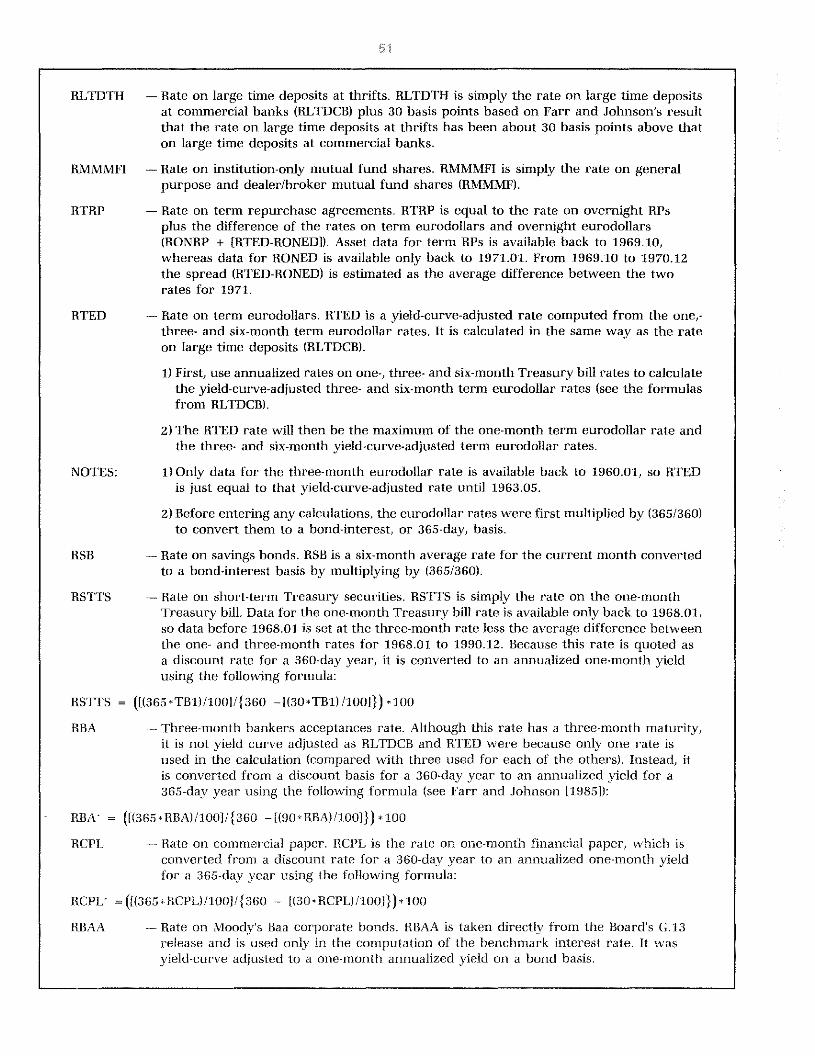
/•.~‘ ~ fl~f4~\.fl (4 ~Surnb?~)41ninand

fl- I

Because the Divisia aggregates are an alterna-tive to the conventional simple-sum aggregates,it is instructive to compare them. When con-structing data in this section, the authors usedan extension of the Farr and Johnson (1985)method. The Appendix presents details of theconstruction of the Divisia monetary aggregatesused here.

A Divisia monetary index is an approximationto a nonlinear utility function. Because it is anindex, the level of utility is an arbitrary unit ofmeasure; the level of the index has no particularmeaning)” Nevertheless, because they are alter-native measures of money, the Divisia and simple-sum aggregates are frequently compared to seehow any analysis of the effects of monetary policyor other issues might be affected by the methodof aggregation. The compar-ison of the levels of

‘1The most widely used test, developed by Varian (1982,19B3), is not statistical. The null hypothesis of weakseparability is rejected if a single violation of the so-calledregularity conditions is found. Because tests for weakseparability lack power, Barnett, Fisher and Serletis (1992,p. 2,095) argue that “existing methods of conducting suchtests are not.. very effective tools of analysis.” See Barnettand Choi (1989) for evidence indicating that available testsof block-wise weak separability are not very dependable.For results of tests for weak separability, see Belongia andChalfant (1989) and Swofford and Whitney (1986, 1987).

“A common practice both in the United States and abroadis to construct Divisia monetary aggregates for collectionsof assets that are reported by the country’s central bank.For example, see Yue and Fluri (1991), Belongia andChrystal (1991) and Ishida (1984).

‘31t should be noted that the accounting stock, that is, thesum of the dollar amounts of all assets that are consideredmoney, is not necessrily equal to the capital stock ofmoney. The accounting stock is the present value of bothservice flow of money and the interest income (the serviceas a store of value). The economic capital stock of money

comprises only the present value of the flow of monetaryservices. See Barnett (1991) for the formula for the economiccapital stock of money.

“For the Divisia monetary aggregates, the share weight ofeach component’s growth rate is its expenditure share oftotal expenditures on monetary services- Theoretically theshare weights for the Divisia monetary aggregates are nota function of prices or user costs, but of quantities. Theobservable user costs are substituted for the unobservablemarginal utilities under the implicit assumption of market-clearing equilibrium, where each consumer holds an optimalportfolio of monetary and nonmonetary assets. For thesimple-sum monetary aggregates, the share weights arethe components’ share of the aggregate.

I’GDMt In DI, — In Dl,~,where DI denotes the Divisiaindex. The index is initialized at 100, that is, D10 = 100.See Farr and Johnson (1985) for more details.

‘“Rotemberg (1991) derives a weighted monetary aggregatestock under conditions of risk neutrality and stationarityexpectations; however, Barnett (1991) shows that thismeasure is the discounted value of future Divisia monetaryservice flows.

39

Figure 1Year-Over-Year Growth of SSM1a and DIVM1a, and Levels of SSM1a and DIVM1a

Feweet

the simple-sum and Divisia measures is made bynormalizing both measures so that they equal 100at some point in the series, usually the first observa-tion.17 Comparisons of the levels and growth ratesof the Divisia and simple-sum measures are pre-sented in figures 1—5 for four monetary aggregates,M1A, Ml, M2 and M3, and for total liquid assets,L.” The figures have two scales, The left-handscale indicates the growth rate, and the right-hand scale indicates the level of the series. Bothindexes equal 100 in January 1960.

.j4~fI

M1A comprises currency and non-interest-bearing demand deposits held by householdsand businesses. Although neither household norbusiness demand deposits earn explicit interest,business demand deposits are assumed to earnan implicit own rate of return proportional tothe rate paid on one-month commercial paper)”Consequently, additional units of businessdemand deposits are assumed to yield a smaller

‘7An alternative justification for comparing the Divisia andsimple-sum aggregates might come from noting that theappropriate Divisia monetary aggregate would be thesimple-sum aggregate if all of the component assets hadidentical own rates. Such a comparison is tenuous, however,because the actual level of the simple-sum aggregatemight have been different from the observed level had theuser costs actually been equal.

It is common to compare the levels and growth rates ofsimple-sum and Divisia monetary aggregates. For example,see Barnett, Fisher and Serletis (1992). Because Divisiaindexes involve logarithms, the growth rate of a componentasset is plus or minus infinity, respectively, when a com-ponent is introduced or eliminated. To circumvent thisproblem, the Divisia index is replaced by Fisher’s idealindex at these times and the user cost is measured by itsreservation price during the period that precedes the intro-duction or follows the elimination of the asset. See Farr

and Johnson (1985) for a discussion of this procedure.“Note that the simple-sum aggregates presented here are

not identical to the official published series. The officialseries are obtained by adding the non-seasonally adjustedcomponents and seasonally adjusting the aggregate as awhole or by adding large subgroups of component assetsthat have been seasonally adjusted as a whole. Thesimple-sum aggregates presented here are obtained byadding the components after each component (that has adistinctive seasonal) has been seasonally adjusted. See theAppendix for details. A comparison of the series used hereand the official series shows that the differences are small.

“Alternatively, estimates of the own rate on household demanddeposits could also be used. However, such a series wasnot available for the entire sample period. Moreover, thedesire was to follow the procedure used by Farr andJohnson (1985) as closely as possible.

Index600

500

400

300

200

100

0

‘4-c

~3 C

0)9,

7-,

‘4CD

0.

‘C 9—

I•

—‘4

o~

I I

0)

N)

0) a 0)

0,

to 0)

N)

0)

0,

-4 0

0) a

N)

~1 0)

-.4 0

a -4 08 08 0

-1 N) -I a -4 0)

08 a

-4 08

08 0 00

N)

41!

08 0)

08 08 to 0 (0 (0 N)

00 a 00 0)

08

00

to 0

3 0.

44

Figure 4Year-Over-Year Growth of SSM3 and DIVM3, and Levels of SSM3 and DIVM3

Fe went

Figure 5Year-Over-Year Growth of SSL and DIVL, and Levels of SSL and DIVL

IIndex

1960 62 64 66 68 70 72 74 76 78 80 82 84 86 88 90 1992

Index1400

1200

1000

800

600

400

200

0

1960 62 64 66 68 70 72 74 76 78 80 82 84 86 88 90 1992

42

flow of monetary services than are additionalunits of household demand deposits. On theother hand, the simple-sum measure implicitlyassumes that each unit of each componentprovides the same flow of monetary services.Hence the Divisia aggregate gives more weightto the growth rates of currency and householddemand deposits than does the simple-sumaggregate.2°

The average differences in the growth ratesof the simple-sum and Divisia measures of MIAfor the entire sample period, January 1960 toDecember 1992, and for selected sub-periodsare presented in table 1. Because currencygenerally grew more rapidly than demanddeposits over the sample period, the growthrate of Divisia M1A averaged about half apercentage point higher than the growth rate ofsimple-sum MIA over the entire period.” Muchof this difference occurs during the latter partof the 1980s, when the growth rate of demanddeposits generally slowed relative to the growthrate of currency.22 This more rapid growth ofthe Divisia measure is reflected in a generallywidening gap between the levels of the indexes.

‘rhe behavior of simple-sum and Divisia Ml issimilar to that of M1A. Indeed, the growth ratesof simple-sum and Divisia Ml were similar untilthe late 1970s, when the growth of interest-bearing NOW accounts began to accelerate. Thesharp rise in NOW accounts after their nationwideintroduction on January 1, 1981, tended toincrease the growth rate of the simple-summeasure relative to the Divisia measure becausethe growth rate of NOW accounts gets a smallerweight in the Divisia measure. As a result, theDivisia measure grew more slowly on average

than the simple-sum measure from the latel970s until the mid-1980s, after growing morerapidly previously. However, in neither periodis the average difference in the growth rate ofthe alternative measures large.”

After the late l9SOs the Divisia measure grewmore rapidly than the simple-sum measure,reflecting the rise in the growth rate of currencyrelative to the growth rate of checkable deposits.Of course, the smaller average difference in thegrowth rates of the alternative Ml aggregatescompared with M1A is reflected in a smallerdifference in the levels of the two indexes as well.

‘4t(t~t t•~

Not surprisingly, larger differences arise whenthe monetary measures are broadened to includesavings-type deposits because their explicit ownrates of return are higher than those of trans-actions deposits. The higher own rate reducesthe share weights of these component assetsrelative to the weights they receive in thesimple-sum measures. During the sample periodthe growth m-ates of the broader simple-sumaggregates tend to be substantially larger thanthose of the corresponding Divisia measures.For the broader measures, the average growthrates of the simple-sum measures are about 2percentage points greater than the correspondingDivisia measures over the entire sample period.

Much of this difference arises from the late1970s to the mid-1980s and is likely due tofinancial innovation and deregulation in theperiod. The late 1970s witnessed a markedacceleration in the growth of money marketmutual funds. These accounts paid relativelyhigh interest rates and had limited transactionscapabilities. A number of new deposit instrumentsthat paid higher market interest rates were

20ln both cases, the sum of the weights must equal unity.21Currency grew at an annual rate of 7 percent during the

entire period, whereas household and business demanddeposits both grew at a 3.2 percent annual rate.

22This is a period of very slow reserve growth. Becausereserves and checkable deposits are tied closely togetherunder the present system of reserve requirements, it is notsurprising that this is also a period of slow growth in check-able deposits, including household and business demanddeposits. See Garfinkel and Thornton (1991) for a discussionof the relationship between reserves and checkable depositsunder the present system of reserve requirements.

“We have refrained from using the phrase “statisticallysignificant” because these observations are clearly dis-tributed identically and independently, so the “t-statistics”reported in table 1 are biased and neither the direction norextent of the bias is known. These statistics are presented

to give the reader a rough approximation of the magnitudeof the differences in the growth rates. Correlegrams of thedifference in the growth rates of simple-sum and Divisia M1Aand Ml show some lower level persistence through thesample period and some large spikes at seasonal frequenciesafter 1969. Correlegrams for the difference in the growthrates of the broader monetary aggregates reveal somehigher level persistence. In any event, differences that aresmall in absolute value tend to be small relative to theestimated standard errors, and differences that are largein absolute value tend to be large in relative terms.

Another measure of the distance between the growthrates is the square root of the sum of the squared differ-ences in the growth rates. These measures for the entiresample period are 58.5, 52.1, 69.6, 81.4 and 77.6 for MIA,Ml, M2, M3 and L, respectively. These data are broadlycomparable with those presented in table 1.

Table 1

Average Percentage Point Difference in the Annual Growth Rate ofSimple-Sum and Divisia Aggregates

Standard

Period Aggregate Mean1 Deviation t-statistic1960.01—1992.07

M1A -0.514 316 3.24~Ml —0.153 283 107M2 1889 3.49 1075’M3 2.317 388 11.88’L 2.223 3.66 1207

1960.01—1977.12M1A —0.285 2.04 205Ml -0253 2.03 182M2 1.660 1.54 15.8’VM3 2134 2.08 l502L 1.897 1.73 16.10’

1978.01—1986.12MIA —0.324 383 0.88Ml 0 420 3.65 1 20M2 3526 5.59 6.55M3 4.334 575 7.84~L 4.303 5.50 8 12

1967.01—1992.12M1A -1 485 4.41 2.85Ml —0.714 332 1.82M2 0.116 2.45 040M3 -0.163 2.82 0.49L 0.076 2.84 0.23

‘The growth rate ol the simple-sum aggregate less the growth rate of the 0iv~siaaggregate.

lndicates a I-stat’stic greater than 2. See footnote 23

iiili’t,iliii’iil iii Ilic t,i,’l~ I~lMlI., i,imI I i.tLlI~llii)IiI) lii iilII\ sItit~i’i’gl’i~\\Ih iii liii’ Iii’mi;uh’, I)i~i.-~i,iinlri’rsl ‘ale i-eiIi’’g’~nile IiI111i4 l)ll.i’.I’mi iimll.~’ ilii’a’,iil’e’. (iill’ll)L~ lIii’~ n’i’iiici N Ilinli’ (‘iiil’~i.—,ti’iiI

\lui’cmi’i’. silmut tel fl illle,’,’—,I ‘alt’.—, ‘c’am’hi’d n itli II,.’ (Iisiflllalli,fl ul liii’ ~rl’U1d lIi,ii, i—, liii’

high li’\i’Is in the ral’l\ I!ISfI~ U tb -,ha,’e g,’un UI ut ti,, —‘unpit—sum aggi’rgiti’s. n bus,’ni’i,~I,l~‘~er1’—lli~m’lii liii’ ‘.pi’i-iml h,’I~~,’c’rian gi’u~~Ill ivilknuivml laid~ ‘amnil. \Iihumigh hi-

un ‘ate 1)1 relin’n intl the l’eltll’ii un gnu lb lilt’s ut’ 11w br, tier’ fli\ i—,ia anil ~implc’—liii lii’iii’iiri,ii’k ,i’,—,tl. it i’, ritil ‘mii’pi’i’.ilim4 thai “niii •u2gi’egile~ hue been es~,’’iliaIIt Ihe ‘.anii’

lii lli~i,i,i liii’i’,tii’i’.’, gr’e\\ ,iiai’l~i’iil~,Iui~~i’, in~ i~i’l’age. .—,i,ii’c’ iluimil him’ iiitI—i!IMt)~lit i’ni’i’espundili4 —ilflpie—,iirir illei’—iIi’i’s palIi’rn ui 41’uu ib uI hi’si’ ,lllel’Ilillfli’ llli’astlli’’,

during iris pu-rind \e~erlheIe-,s the ~ignI— is surn,’n hal dilit’n,it

- -ro’ discuss on of lhc fin,mncia’ innovations of this periods’ C Ci.aerl t 1q66) nj Stone a’o Tno’n:or 11991)

44

A. (]onq.n.nAson of .Broat.h.o’ .I.Jit.•~IAiA

That Divisia aggregation gives relatively small

weight to less liquid assets that yield high ratesof return suggests that differences in the growthrates of successively broader Divisia monetaryaggregates will tend to get smaller.” The levelsof Divisia M2, M3 and L presented in figure 6and simple correlations of the compoundedannual growth rates of these Divisia aggregatespresented in table 2 confirm this. The growthrates of Divisia M3 and L differ little from thegrowth i-ate of Divisia M2. This implies that addingsuccessively less liquid assets to those in M2 addslittle to the flow of monetary services.” That theaverage difference in the growth rates of Divisia

M2 and L is nearLy zero over the entire sample

period is reflected by the levels of the two Divisiaaggregates, which are essentially equal by the endof the samnple. Divisia M3, however, has grownmore rapidly than the other measures, so thespread between its level and the levels of DivisiaM2 and L has widened over the sample period.

(.X.JNCLUDI}.VG RETIIAI.tKS

Despite their theoretical advantage, Divisiaand other weighted monetary aggregates havegarnered relatively little attention outside ofacademe, and the official U.S. monetary aggregatesremain simple-sum aggregates. The officialreliance on simple-sum aggregates will probablycontinue unless the Divisia aggregates or otheralter-native weighted aggregates are shown to besuperior in economic and policy analysis.

250f course this tendency also exists for the simple-sumaggregates. For the simple-sum aggregate, the growth rateof each component is weighted by the components shareof the total asset. Hence the growth rates of successivelybroader monetary aggregates could diverge if the marginalcomponents were successively larger. For example, this iswhat happens from Ml to M2. The growth rates tend toconverge, however, because the marginal components aresmaller. This tendency is exacerbated in the Divisia

measures because of smaller weights associated withhigher own rates of return on successively less liquid assets.

“The average differences in the growth rates of Divisia M2,M3 and L over the sample period are small (less than 0.12percentage points in absolute value). The absolute valuesof the average differences in the growth rates of simple-sum M2, M3 and L are larger than those of the correspondingDivisia measures; the standard errors are also much larger.

Figure 6Levels of Divisia M2, M3, and L

Index

1960 62 64 66 68 70 72 74 76 78 80 82 84 86 88 90 1992

Table 2

Correlations of the Annual GrowthRates of the Divisia MonetaryAggregates

Aggregate M1A Ml M2 M3

Ml 7920

M2 6540 .6914

M3 .6015 .6346 9568

L .5754 6126 .8863 .9216

.~Iihungh huh lung del roilhe ram lie saki aboutthis issue from the simple analysis of the datapresented here, a few observations are offered.

First, that the growth rates of the narrow simple-sum and Divisia monetary aggregates are quitesimilar suggests that the method of aggregationmay not be important at low levels of aggregation.~~For example, it does not appear that conclusionsabout the long-run effects of money growth oninflation would be much different using eithersimple-sum or Divisia Ml or M1A. The averagedifference in the growth rates of narrow simple-sum arid Divisia monetary aggregates is small.This observation is consistent with the empiricalwork of Barnett, Offenbacher and Spindt (1984)who, using a broad array of criteria, found thatthe difference in the performance of simple-sumand Divisia mnonetary aggregates was small atlow levels of aggregation.

Second, the method of aggregation is likely to bemore important for broader monetary aggregates.Beyond some point, however, a further broadening

of the monetary aggregate makes little difference.Fom the United States, the differences in theaverage growth rates of Divisia M2, M3 and Lare small. Consequently, long-run analysis usingthe growth rates of any of these Divisia aggregatesis likely to produce similar results. Monthlygrowth rates of these Divisia aggregates are also

highly correlated. Hence it would not be toosurprising to find that the broader Divisiaaggregates perform similarly to one anothem- inmany short-run analyses as well.

These observations point to the critical needfor more work to determine which financial

assets should be included in the appropriatemonetary aggregate. In consumer demandtheory, these assets must satisfy the conditionof weak separability. If analysis suggests arelatively narrow monetary aggregate such asMl, policymakers may be reluctant to adopt thetheoretically superior index measure because, asa practical matter, the method of aggregationmay not be empirically important.

If such tests point to an aggregate that includesa much broader array of financial assets, thepractical case for the weighted aggregates willbe enhanced. Even casual analysis of simple-sum and Divisia monetary aggregate data showdifferences in both the levels and growth ratesof these aggregates that are large, suggestingthat the mnethod of aggregation is important.Consequently, the method of aggregation shouldalso be a concern for those who favor broadermonetary aggregates on other grounds. Theobjective of the present article in publishingDivisia monetary statistics is to stimulate furtherempirical research both on the importance ofmonetary aggregation and on the role of moneyin the economy.

I.1F:FEI.IE:.)\A]ES

Barnett, William A., Douglas Fisher and Apostolos Serletis.“Consumer Theory and the Demand for Money,” Journalof Economic Literature (December 1992), pp. 2,086—119.

Barnett, William A. Reply,” in Michael T. Belongia, ed.,Monetary Policy on the 75th Anniversary of the FederalReserve System (Kluwer Academic Publishers, 1991),pp. 232—42.

Bamnett, William A., and Seungmook Choi, “A Monte CarloStudy of Tests of Blockwise Weak Separability,” Journal ofBusiness and Economic Statistics (July 1989), pp. 363—79.

Barnett, William A., Edward K. Offenbacher and Paul A.Spindt. ‘The New Divisia Monetary Aggregates,” Journalof Political Economy (December 1984), pp. 1,049—85.

Barnett, William A. “Economic Monetary Aggregates: AnApplication of Index Number and Aggregation Theory,”Journal of Econometrics (September 1980), pp. 11—48.

Belongia, Michael T., and K. Alec Chrystal. ‘An AdmissibleMonetary Aggregate for the United Kingdom,” Review ofEconomics and Statistics (August 1991), pp. 491—502.

Belongia, Michael T., and James A. Chalfant. ‘The ChangingEmpirical Definition of Money: Some Estimates from aModel of the Demand for Money Substitutes,” Journal ofPolitical Economy (April 1989), pp. 387—97.

Chetty, V. Karuppan. “On Measuring the Nearness of Near-Moneys,” American Economic Review (June 1969),pp. 270—81.

Farr, Helen T., and Deborah Johnson. “Revisions in theMonetary Services (Divisia) Indexes of Monetary Aggregates,”Staff Study 147, Board of Governors of the Federal ReserveSystem (1985).

27There may be some differences in the levels, however,because the levels of the simple-sum and Divisia

measures do not appear to be cointegrated at any level ofaggregation-

Feenstra, Robert C. “Functional Equivalence betweenLiquidity Costs and the Utility of Money,” Journal ofMonetary Economics (March 1986), pp. 271—91.

Feige, Edward L. The Demand for Liquid Assets: A TemporalCross-Section Analysis, (Englewood Cliffs, 1964).

Fisher, Douglas. Money Demand and Monetary Policy,(University of Michigan Press, 1989).

Fisher, Irving. The Making of Index Numbers: A Study of TheirVarieties, Tests, and Reliability, (Houghton Mitflin, 1922).

The Purchasing Power of Money (Augustus M.KeIley, 1911).

Garfinkel, Michelle R., and Daniel L. Thornton. “TheMultiplier Approach to the Money Supply Process: APrecautionary Note,” this Review (JulylAugust 1991),pp. 47—64.

Gilbert, A. Alton. “Requiem For Regulation 0: What It Didand Why It Passed Away,” this Review (February 1986),pp. 22—37.

Gurley, John G. and Edward S. Shaw. Money in a Theory ofFinance, (Brookings Institution, 1960).

lshida, Kazuhiko. “Divisia Monetary Aggregates and Demandfor Money: A Japanese Case,” Bank of Japan Monetaryand Economic Studies (June 1984), pp. 49—80.

Laidler, David - Taking Money Seriously and Other Essays,(MIT Press, 1990).

Mason, Will E. ‘The Empirical Definition of Money: ACritique,” Economic Inquiry (December 1976), pp. 525—38.

Pesek, P. Boris, and Thomas A. Saving. Money, Wealth andEconomic Theory (The MacMillan Company, 1967).

Rotemberg, Julio J., “Monetary Aggregates and Their Uses,”in Michael T. Belongia, ed., Monetary Policy on the 75thAnniversary of the Federal Reserve System (KluwerAcademic Publishers, 1991), pp. 223—31.

Spindt, Paul A. “Money is What Money Does: MonetaryAggregation and the Equation of Exchange,” Journal ofPolitical Economy (February 1985), pp. 175—204.

Stone, Courtenay C., and Daniel L. Thornton. ‘FinancialInnovation: Causes and Consequences,” in Kevin Dowdand Mervyn K. Lewis, eds., Current /ssues in MonetaryAnalysis and Policy, (MacMillan Publishers, 1991).

Swofford, James L., and Gerald A. Whitney. “NonparametricTests of Utility Maximization and Weak Separability forConsumption, Leisure and Money,” Review of Economicsand Statistics (August 1987), pp. 458—64.

_______- “Flexible Functional Forms and the Utility Approachto the Demand for Money: A Nonparametric Analysis,”Journal of Money, Credit and Banking (August 1986),pp. 383—89.

Varian, Hal A, “Non-Parametric Tests of Consumer Behavior,”Review of Economic Studies (January 1983), pp. 99—110.

_______- “The Nonparametic Approach to Demand Analysis,”Econometrica (July 1982), pp. 945—73.

Yue, Piyu. “A Microeconomic Approach to Estimating MoneyDemand: The Asymptotically Ideal Model,” this Review(NovemberlDecember 1991a), pp. 36—51.

_______- Theoretic Monetary Aggregation Under Risk AversePreferences, IC2 Institute (University of Texas at Austin,1991b).

Vue, Piyu, and Robert Fluri. “Divisia Monetary ServicesIndexes for Switzerland: Are they Useful for MonetaryTargeting?” this Review (September/October 1991),pp. 19—33.

(kins~truc:tIng :ijivisia r%v5:,r’ ~:~tAi•.r1v0~

The assets used to calculate Divisia monetaryaggregates are the same as those used by the Boardof Governors to calculate the official simple-sumaggregates MIA through L. The only major dif-ference is that demand deposits are broken intohousehold demand deposits (HDD) and businessdemand deposits (BDD). We assume that house-holds receive a zemo rate of return on demanddeposits and that businesses receive an implicit,nonzero rate of return. HDD and BDD are com-puted using seasonally adjusted monthly data fortotal demand deposits and non-seasonally adjustedquarterly data for consumer, foreign, financial,nonfinancial and other demand deposits. Thesecan be found in Table 1.31 of the Federal ReserveBulletin. Using the non-seasonally adjusted quarterly

data, we calculate two ratios and use them to par-

tition the seasonally adjusted monthly data. The ratiofor BDD is the sum of financial and nonfinancialdemand deposits divided by the sum of all fivenon-seasonally adjusted series, whereas the ratiofor HDD is one minus the BDD ratio. The non-seasonally adjusted series go back only to 1970,01and are discontinued after 1990.06. For data before1970.01 and after 1990.06, the means of the re-spective ratio series over the available samplewere used. The means used were 62.33 percentfor BDD and 37.67 percent for HDD. To get thefinal HDD and BDD series, these quarterly ratioswere multiplied by the seasonally adjusted monthlydata for total demand deposits. Each quarterlyobservation was multiplied by the three monthsof data for that particular quarter. All assets areseasonally adjusted and in millions of dollars.

1The Divisia monetary aggregates data presented herewere constructed under the direction of Piyu Vue. Lynn D.

Dietrich and Kevin L. Kliesen gathered the data, wrote thecomputer code and wrote this appendix.

;~/o0~ t:.no•~en1~s

CUR — Sum of seasonally adjusted currency and traveler’s checks.

DEMDPS — Total demand deposits.

HDD — Demand deposits for households as described in the preceding section.

BDD — Demand deposits for businesses as described in the preceding section.

OCD — Other checkable deposits less super NOW account balances. OCD includes ATS andNOW balances, credit union share draft balances and demand deposits at thrift insti-tutions.

SNOWC — Super NOW accounts at commercial banks. SNOWC data begin in 1983.01 and end in1986.03. After 1986.03 there is no distinction between NOWs and super NOWs.

SNOWT — Super NOW accounts at thrifts. SNOWT begin in 1983.01 and end in 1986.03. After1986.03 there is no distinction between NOWs and super NOWs.

ONRP — Overnight repurchase agreements. ONRP includes overnight and continuing contractrepurchase agreements issued by commercial banks to organizations other than depositoryinstitutions and money market mutual funds (MMMF5) (general purpose and broker/dealerorganizations) -

ONED — Overnight eurodollars. ONEDs are issued by foreign (principally Caribbean and London)branches of U.S. banks to U.S. residents and organizations other than depositoryinstitutions and money market mutual funds.

MMMF — Money market mutual funds. MMMF is general purpose and broker/dealer money marketmutual fund balances including taxable and tax-exempt funds and excluding IRA/KEOGH

accounts at money funds.

MMDAC — Money market deposit accounts at commercial banks. MMDAC initially had a minimumbalance requirement of $2,500 until December 31, 1984, and a $1,000 minimum balancerequirement until December 31, 1985, when the requirement was removed. MMDACswere no longer reported after 1991.08.

MMDAT — Money market deposit accounts at thrifts. MMDAT initially had a minimum balancerequirement of $2,500 until December 31, 1984, and a $1,000 minimum balancerequirement until December 31, 1985, when the minimum requirement was removed.MMDATs were no longer reported after 1991.08.

SDCB — Savings deposits at commercial banks less money market deposit accounts at commercialbanks. MMDACs are included after 1991.08.

SDSL — Savings deposits at thrifts Tess money market deposit accounts at thrifts. MMDATs areincluded after 1991.08.

STDCB — Small time deposits (less than $100,000) at thrifts including retail repurchase agreementsless IRA/KEOGH accounts.

STDTH — Small time deposits (less than $100,000) at thrifts including retail repurchase agreementsless IRA/KEOGH accounts.

LTDCB — Large time deposits (more than $100,000) at commercial banks excluding internationalbanking facilities (IBFs).

LTDTH — Large time deposits (more than $100,000) at thrifts excluding IBFS.

MMMFI — Institution only money market mutual funds. MMMFI includes taxable and tax-exemptfunds and excludes IRA/KEOGH accounts at money funds.

TRP — Term repurchase agreements. TRP consists of RPs with original maturities greater thanone day, excluding continuing contracts and retail RPs.

48

TED

SB

SiTS

BA

CP

— Term eurodollars with original maturities greater than one day. TED includes thoseeurodollars issued to U.S. residents by foreign branches of U.S. banks and by allbanking offices in the United Kingdom and Canada. Eurodollars held by depository in-stitutions and MMMFs are not included.

— Savings bonds.

— Short-term Treasury securities. STTS comprises U.S. Treasury bills and coupons withremaining maturities of less than 12 months not held by depository institutions, Fed-eral Reserve Banks, MMMFs or foreign entities.

— Bankers acceptances. BA is the net of bankers acceptances held by accepting banks,Federal Reserve Banks, foreign official institutions, federal home loan banks and MMMFs.

— Total commercial paper less commercial paper held by MMMFs.

The interest rate data are more complicatedthan the asset data. The major concern with theinterest rate data is the variety of forms inwhich they are reported. Before including dif-ferent rates in an aggregate, the characteristicsof all the rates should be as similar as possible.To this end, two problems need to be addressed.First, for composite asset stocks where thetotal asset is the sum of deposits with differentmaturities, such as small and large time de-posits, the own rate is the maximum ratepaid across the deposit categories at eachpoint.

Because there are a variety of maturity lengthsamong the rates of a given composite asset stock,an adjustment is needed to transform each rateto a common maturity before the final rate iscomputed. Given rates with differing maturitiesand a typical upward-sloping yield curve, liquiditypremiums keep rates on assets with longermaturities higher than rates on those with shortermaturities. To adjust these rates to a commonmaturity, this liquidity premium must be removedusing a yield curve adjustment as described inFarr and Johnson (1985). As Farr and Johnsondid, all rates that are yield curve adjusted areadjusted to a one-month maturity:

R — (TBM—TBI), where

R = the original rate on a bond basis (that is,a 365-day basis) basis

= the yield curve adjusted rate

TBM = the M-month Treasury bill rate

TB, = the one-month Treasury bill rate

A second adjustment is needed to convert allthe rates to the same yield basis. Interest ratesare quoted in various forms, including discountbasis and annual percentage rate basis, and havevarious interest bases, including bond (365 day)and bank (360 day). To the extent possible, therates were transformed into annualized one-monthinvestment yields on a bond-interest basis. Forrates quoted on a discount basis for a 360-dayyear, the following formula can be used to convertthem to an annualized yield for a 365-day year(see Farr and Johnson [1985]):

R (u36s~D/1oo]/ {36o_[N*D)/loo]}) * 100,

where R = the annualized rateD = a discount basis rate (360-day year)N = the number of days to maturity

Including the variable N ensures that the formu-la is maturity independent.

11;’ trTFtSt Hate :%(•~r1i::~.Sl(ir tat? .tflfl..ttrl•T)ifl/Jt)flt?flS

RZER

RDD 1

RDD2

— Rate on currency and traveler’s checks. RZER is zero by definition.

— Rate on household demand deposits. RDDI is zero by definition.

— Rate on business demand deposits. The basic formula for computing is as follows:

RDD2 = (1-MRrn~RCp

where MRR = maximum reserve requirement on demand depositsRCP = one-month financial paper rate

Before applying this formula, adjust RCP, which is quoted on a discount basis for a360-day year, to an annualized one-month yield for a 365-day year. This is done byusing the formula described in the preceding text.

49

RCP’ = ([(365 * RCP)/100]/{360 — [(3o.RCP)/loo]}) * 100

Then RDD2 = (1_MRR)*RCP

For MRR and all ceiling rates used in the following text, we use the same conven-tion as Farr and Johnson and assume that rates are quoted as annualized one-monthyields.

ROCD — Rate on other checkable deposits.

1960.01—1974.11 — Regulation Q ceiling rate on passbook savings accounts at commercialbanks. From t962.01—1964,12 the ceiling rate on savings deposits ofless than 12 months is used.

1974.12—1986.03 — Regulation Q ceiling rate on NOW accounts.

1986.04—present — Weighted average interest rate on NOWs and super NOWs.

RSNOWC — Rate on super NOWs at commercial banks. RSNOWC is the average rate paid on superNOW accounts at insured commercial banks and is quoted on an effective annual yieldin the monthly Survey of Selected Deposits, a special supplementary table in the weeklyFederal Reserve Statistical Release H.6.

RSNOWT — Rate on super NOWs at thrift institutions. RSNOWT is the average rate paid on superNOW accounts at FDIC-insured savings banks (both mutual and federal savings banks)and is quoted on an effective annual yield in the monthly Survey of Selected Deposits,a special supplementary table in the weekly Federal Reserve Statistical Release HG.

RONRP — Rate on overnight dealer financing in the repurchase market. Because RONRP is anovernight rate quoted on a bank-interest basis, it must be transformed into an annualizedone-month yield on a bond-interest basis using the following formula:

RONRP* = {[i + (RONRP/36000)]~°—1 } *(3~5~JQ/3ffl

Data for RONRP goes back only to 1972.01, whereas asset data goes back to 1969.11.Farr and Johnson argue that the rate on overnight RPs has historically been five basispoints below the federal funds rate, so we use the following formula to compute a rate

before 1972:

RONRP* = ({[1+(RFF/3G000)]3o_1}*(36soo/3ffl) —.05

Like RONRP, the fed funds rate is an overnight rate quoted on a discount basisand must be transformed into an annualized one-month yield on a bond-interestbasis.

RONED — Rate on overnight eurodollars from London. The original series is weekly, and thus themonthly series is a simple average of the weekly observations for a particular month. LikeRONRP, RONED is an overnight rate quoted on a bank-interest basis and must be con-verted to an annualized one-month yield on a bond-interest basis using the followingformula:

RONEDt= {Ei + (RONED/36oo0)]~°— I } * (36500/30)

RMMMF — Average yield of money market mutual funds. RMMMF comes from the Board, whichin turn gets it from Donoghue~sMoney Fund Reporl. Data for RMMMF is available onlyback to 1974.06. RMMMF data from before this date are set to the rate on large timedeposits at commercial banks (RLTDCB) less 70 basis points (see Farr and Johnson[1985]).

RMMDAC — Rate on money market deposit accounts at commercial banks. Before 1989.06 RMMDACis the average rate paid at insured commercial banks. After 1989.07 it is the averageof the rates paid at insured commercial banks for personal and nonpersonal MMDAs,which are quoted as effective annual yields in the monthly Survey of Selected Deposits,a special supplementary table in the weekly Federal Reserve Statistical Release H.6.

RMMDAT — Rate on money market deposit accounts at thrift institutions. Before 1989.06 RMMDATis the average rate paid at FDIC-insured savings banks. After 1989.07 it is the averageof the rates paid at FDIC-insured savings banks (including both mutual and federalsavings banks) for personal and nonpersonal MMDAs, which are quoted as effectiveannual yields in the monthly Survey of Selected Deposits, a special supplementary ta-ble in the weekly Federal Reserve Statistical Release H.6.

RSDCB — Rate on savings deposits at commercial banks less money market deposit accounts atcommercial banks. RSDCB comes from the Board and is quoted as an effective annual yield.

RSDSL — Rate on savings deposits at FDIC-insured savings banks (the thrift rate).

1966.10—1986.03 — The ceiling rate on NOW accounts at thrifts.

1986.04—present — The rate on savings deposits at thrifts published in the Board’s H.6release.

There are two problems with data before 1966.10: 1) interest rates on savings depositsat thrifts were not regulated and 2) different states paid different rates on these accounts.One of the few series published for this period is the average dividend paid on savingsdeposits at thrifts, which is what we use here. This is an annual rate and includespassbook savings aecounts and fixed-term certificates.

FITSTCB — Rate on small time deposits and retail repurchase agreements at commercial banks.FITSTCB is the Fitzgerald-adjusted small time deposit rate that is calculated at the Boardand quoted as an effective annual yield.

RSTTH — Rate on small time deposits and retail repurchase agreements at thrifts. RSTTH is theFitzgerald-adjusted small time rate that is calculated at the Board and quoted as an ef-fective annual yield.

RLTDCB — Rate on large time deposits at commercial banks. RLTDCB is a yield-curve-adjusted ratethat is calculated using the one-, three- and six-month secondary CD rates (of depositsgreater than $100,000) and the one-, three- and six-month Treasury bill rates.

1) The first step is to convert the Treasury bill rates, which are quoted on a discountbasis for a 360-day year, to annualized yields for a 365-day year as follows:

= ([(365*Y)/loo]/{36o_[(N*Y)/loo]}) *100

where Y = one-, three- and six-month Treasury bill rates on a discount basisN = number of days to maturity

2) Second, calculate the yield-curve-adjusted three- and six-month CD rates using thefollowing formula:

RCD3YCA = RCD3 - (Y3-Y1)RCD6YCA = RCD6 - (Y6-Y1)

where RCD3 = three-month CD rateRCD6 = six-month CD rate

Yl = one-month Treasury bill rateY3 = three-month Treasury bill rate

3) Finally, the interest rate for large time deposits at commercial banks is given asfollows:

RLTDCB — MAX (RCD1, RCD3YCA, RCD6YCA).

I) Data on CD rates were not available before 1964.06 50 RLTDCB was set to the ceilingrate on savings deposits of less than one year as set by Regulation Q.

2) Before entering any calculations, the CD rates were multiplied by (365/360) to convertthem to a bond, or 365-day, basis.

RLTDTH — Rate on large time deposits at thrifts. RLTDTH is simply the rate on large time depositsat commercial banks (RLTDCB) plus 30 basis points based on Farr and Johnson’s resultthat the rate on large time deposits at thrifts has been about 30 basis points above thaton large time deposits at commercial banks.

RMMMFI — Rate on institution-only mutual fund shares. RMMMFI is simply the rate on generalpurpose and dealer/broker mutual fund shares (RMMMF).

RTRp — Rate on term repurchase agreements. RTRP is equal to the rate on overnight RPsplus the difference of the rates on term eurodollars and overnight eurodollars(RONRP + [RTED-RONED]). Asset data for term BPs is available back to 1969.10,whereas data for HONED is available only back to 1971.01. From 1969.10 to 1970.12the spread (RTED-RONED) is estimated as the average difference between the tworates for 1971.

RTED — Rate on term eurodollars. RTED is a yield-curve-adjusted rate computed from the one,-three- and six-month term eurodollar rates. It is calculated in the same way as the rateon large time deposits (RLTDCB).

1) First, use annualized rates on one-, three- and six-month Treasury bill rates to calculatethe yield-curve-adjusted three- and six-month term eurodollar rates (see the formulasfrom RLTDCB).

z) The RTED rate will then be the maximum of the one-month term eurodollar rate andthe three- and six-month yield-curve-adjusted term eurodollar rates.

NOTES: 1) Only data for the three-month eurodollar rate is available back to 1960.01, so RTEDis just equal to that yield-curve-adjusted rate until 1963.05.

2) Before entering any calculations, the eurodollar rates were first multiplied by (365/360)to convert them to a bond-interest, or 365-day, basis.

RSB — Rate on savings bonds. RSB is a six-month average rate for the current month convertedto a bond-interest basis by multiplying by (365/360).

RSTTS — Rate on short-term Treasury securities. RSTTS is simply the rate on the one-monthTreasury bill. Data for the one-month Treasury bill rate is available only back to 1968.01,so data before 1968.01 is set at the three-month rate less the average difference betweenthe one- and three-month rates for 1968.01 to 1990.12. Because this rate is quoted asa discount rate for a 360-day year, it is convened to an annualized one-month yieldusing the following formula:

RSTTS = ([365*TBfl/loo]/{36o _[(30*TB1) /ioo]}) *100

RBA — Three-month bankers acceptances rate. Although this rate has a three-month maturity,it is not yield curve adjusted as RLTDCB and RTED were because only one rate isused in the calculation (compared with three used for each of the others). Instead, itis converted from a discount basis for a 360-day year to an annualized yield for a365-day year using the following formula (see Farr and Johnson [1985]):

RBA = (u365*RBA/lool/{36o _[(90*RBA)/100]}) *100

RCPL — Rate on commercial paper. RCPL is the rate on one-month financial paper, which isconverted from a discount rate for a 360-day year to an annualized one-month yieldfor a 365-day year using the following formula:

RCPL’ = ([(363*RCPL)/190]/{36Q — [(30*RCPL)/100]}) 100

RBAA — Rate on Moody’s Baa corporate bonds. RBAA is taken directly from the Board’s G.13release and is used only in the computation of the benchmark interest rate. II wasyield-curve adjusted to a one-month annualized yield on a bond basis.

BENCH — BENCH is the highest yielding rate for the period among all 24 interest rate series andthe Baa bond rate; that is,

BENCH = MAX [RBAA, (Ri,, i = I 24)].

Simple-sum and Divisia monetary aggregates presented in this article can be downloaded from theFRED electronic bulletin board with a personal computer and a modem. The monetary aggregatesare in a file called “DIViSIA.” To access FRED, dial 314-621-1824. Parameters for communicationsoftware should be set to no parity, word length = 8 bits, one stop bit, full duplex and the fastestbaud rate your modem supports, up to 9,600 bps. For more information, telephone Tom Pollmannat 314-444-8562.