Alternative Methods for Sorting Large Files without ... · 1 Alternative Methods for Sorting Large...
23
1 Alternative Methods for Sorting Large Files without leaving a Big Disk Space Footprint Rita Volya, Harvard Medical School, Boston, MA ABSTRACT Working with very large data is not only a question of efficiency but also of feasibility. How often have you received an error message indicating that “no disk space is available”? In many cases this message is caused by the procedure sorting your data. PROC SORT requires three to four times the space needed for data storage. This may be a problem when SAS © work space is limited or shared by many users. This article addresses alternative methods of sorting data without leaving a big footprint on the disk space. Medical claims processing for health care research will illustrate methods. INTRODUCTION Disk space and processing power have grown tremendously over the last two decades, facilitating research across a wide variety of settings. During this period, however, data acquisition technologies have also improved dramatically. Databases have grown from a few million records to hundreds of millions of records. Processing such data can be challenging, not only due to size, but also due to competing demands for computer resources. Too often, the system slows and jobs crash because of a lack of work disk space. One of the fundamental data processing tasks, sorting the data, is often the source of the problem. In this paper, methods to improve PROC SORT performance and alternative methods to sort the data while avoiding a large work disk space footprint are presented. This paper will: Discuss common ways of sorting data Show the problems that might occur while sorting very large data Provide alternative methods that can solve the disk space problem Discuss use of resources by different methods: processing time, disk space, memory. EXAMPLE Suppose data called CLAIMS with multiple records per person are available. These data may represent medical records for every visit of a patient to a health care provider. Also assume that there is another data set, denoted PEOPLE, with a single record per patient. This file represents people selected for an analysis. The data set CLAIMS has many variables for patients that exist in the data set PEOPLE and the goal is to summarize these variables.
Transcript of Alternative Methods for Sorting Large Files without ... · 1 Alternative Methods for Sorting Large...

1
Alternative Methods for Sorting Large Files without leaving a Big Disk Space Footprint
Rita Volya, Harvard Medical School, Boston, MA
ABSTRACT
Working with very large data is not only a question of efficiency but also of feasibility. How often
have you received an error message indicating that “no disk space is available”? In many cases
this message is caused by the procedure sorting your data. PROC SORT requires three to four
times the space needed for data storage. This may be a problem when SAS© work space is limited
or shared by many users. This article addresses alternative methods of sorting data without leaving
a big footprint on the disk space. Medical claims processing for health care research will illustrate
methods.
INTRODUCTION
Disk space and processing power have grown tremendously over the last two decades, facilitating
research across a wide variety of settings. During this period, however, data acquisition
technologies have also improved dramatically. Databases have grown from a few million records to
hundreds of millions of records. Processing such data can be challenging, not only due to size, but
also due to competing demands for computer resources. Too often, the system slows and jobs
crash because of a lack of work disk space.
One of the fundamental data processing tasks, sorting the data, is often the source of the problem.
In this paper, methods to improve PROC SORT performance and alternative methods to sort the
data while avoiding a large work disk space footprint are presented.
This paper will:
Discuss common ways of sorting data
Show the problems that might occur while sorting very large data
Provide alternative methods that can solve the disk space problem
Discuss use of resources by different methods: processing time, disk space, memory.
EXAMPLE
Suppose data called CLAIMS with multiple records per person are available. These data may
represent medical records for every visit of a patient to a health care provider. Also assume that
there is another data set, denoted PEOPLE, with a single record per patient. This file represents
people selected for an analysis. The data set CLAIMS has many variables for patients that exist in
the data set PEOPLE and the goal is to summarize these variables.

2
Data set
CLAIMS has:
ID. This is the first key, a character variable 32 bytes long. This represents a patient ID.
Usually an ID can fit in a field of no more than 15 bytes but, for the feasibility of the task,
an extreme case is selected.
SRV_BGN_DT and SRV_END_DT. These are two numeric variables occupying 16
bytes (service start date and service end date); together they form the second key.
There may be more fields in the second composite key but two are selected for
illustration.
Other fields. These represent additional variables in the data and occupy 1,000 bytes.
71,000,000 records occupying 74 GB.
Data set PEOPLE has:
ID. This is a character variable 32 bytes long
58,000 records
The data is sorted by ID.
TASK
The task consists of sorting the data set CLAIMS by the first key or by the first and second
composite keys, or sorting and then merging data CLAIMS and data PEOPLE. These are very
common tasks that hardly any program can avoid. The methods described in this paper can be
used to solve the first task, the second task, or both.
Data PEOPLE might have other variables. These variables might be intended to be kept in the final
merged data. The algorithms below have to be modified to accomplish this task.
All the jobs were run using SAS 9.3 on SunOS 5.10 (SUN X64) platform. The processing times
reported provide a perspective on the performance and are not meant to compare efficiencies.
USE OF RESOURCES
There are several ways to track the use of resources including the use of memory. The SAS©
System provides the FULLSTIMER option to collect performance statistics on each SAS step, and
for the job as a whole, and places them in the SAS log. The statistics include real time, user and
system CPU times, memory used, memory available and more. To determine how much memory
is available, use the function GETOPTION() like in the DATA step below.
data _null_;
format _memsize_ comma20.;
_memsize_= input(getoption('xmrlmem'),20.);
3
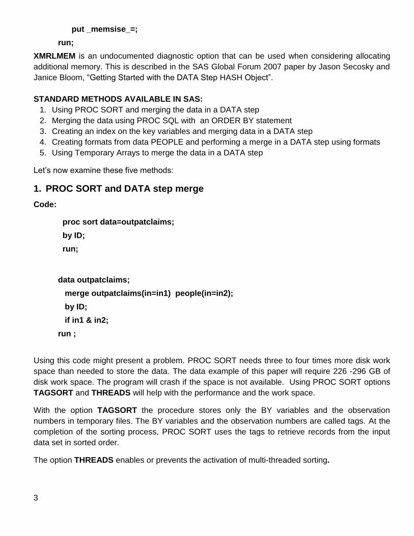
put _memsise_=;
run;
XMRLMEM is an undocumented diagnostic option that can be used when considering allocating
additional memory. This is described in the SAS Global Forum 2007 paper by Jason Secosky and
Janice Bloom, “Getting Started with the DATA Step HASH Object”.
STANDARD METHODS AVAILABLE IN SAS:
1. Using PROC SORT and merging the data in a DATA step
2. Merging the data using PROC SQL with an ORDER BY statement
3. Creating an index on the key variables and merging data in a DATA step
4. Creating formats from data PEOPLE and performing a merge in a DATA step using formats
5. Using Temporary Arrays to merge the data in a DATA step
Let’s now examine these five methods:
1. PROC SORT and DATA step merge
Code:
proc sort data=outpatclaims;
by ID;
run;
data outpatclaims;
merge outpatclaims(in=in1) people(in=in2);
by ID;
if in1 & in2;
run ;
Using this code might present a problem. PROC SORT needs three to four times more disk work
space than needed to store the data. The data example of this paper will require 226 -296 GB of
disk work space. The program will crash if the space is not available. Using PROC SORT options
TAGSORT and THREADS will help with the performance and the work space.
With the option TAGSORT the procedure stores only the BY variables and the observation
numbers in temporary files. The BY variables and the observation numbers are called tags. At the
completion of the sorting process, PROC SORT uses the tags to retrieve records from the input
data set in sorted order.
The option THREADS enables or prevents the activation of multi-threaded sorting.

4
Performance:
Without additional options:
PROC SORT:
real time 38:33.60
cpu time 12:08.60
DATA Step Merge:
real time 3:31.81
cpu time 2:09.41
With Options TAGSORT and THREADS:
PROC SORT:
real time 70:33:54.80
cpu time 2:26:00.65
DATA Step Merge:
real time 4:28.48
cpu time 2:47.23
The option TAGSORT did not provide a good solution in terms of performance to reduce disk
space usage.
2. Merging the data using PROC SQL with an ORDER BY statement
Code:
option msglevel = i ;
proc sql _method ;
create table outpatclaims_sorted
as select *
from people (sortedby = ID) p,
outpatclaims_notsorted op
where p.ID= op.ID
ordered by p.ID , SRVC_BGN_DT, SRVC_END_DT;
quit ;
PROC SQL is generally more efficient than PROC SORT but requires a lot of work disk space to
perform the sorting. The example above uses option _METHOD in a PROC SQL statement. This
option generates a statement in a log file and lists the methods used to sort the data:

5
Sample from log file:
NOTE: SQL execution methods chosen are:
sqxcrta
sqxsort
sqxjhsh
sqxsrc(WORK.PEOPLE(alias = P))
sqxsrc(WORK.OUTPATCLAIMS_NOTSORTED(alias = D))
PROC SQL needs the same or more disk space as PROC SORT and will crash if space is not
available. It is important to use the option SORTEDBY= to tell PROC SQL that the data set
PEOPLE is sorted in order of the keys so that the resources are not wasted on re-sorting the data.
The following table summarizes the methods PROC SQL uses. The table makes clear that the
merge is generated using the hashing method but is separate from a sorting routine. That is where
Hash objects, discussed later in this paper, might not only save disk space but be more efficient
than PROC SQL.
_Method Option Codes Descriptions
SQXCRTA Create table as Select
SQXSLCT Select statement or clause
SQXJSL Step loop join (Cartesian)
SQXJM Merge join operation
SQXJNDX Index join operation
SQXJHSH Hash join operation
SQXSORT Sort operation
SQXSRC Source rows from table
SQXFIL Rows filtration
SQXSUMG Summary stats (aggregates) with GROUP BY clause
SQXSUMN Summary stats with no GROUP BY clause

6
PROC SQL chooses a method depending on the size of the tables involved (the approximate logic
of the choices below is described in Kent [8]):
Indexed if there are any candidate indexes
Merge If one or both of the data sets are already sorted in a convenient sort order
Hash if one of the data sets will fit into memory. Actually, if only 1% of the data set fits in
a single memory extent whose size is the SQL buffersize (64000 bytes), PROC SQL
choses Hash.
Otherwise PROC SQL will choose to sort the incoming datasets and perform the
Sort/Merge algorithm to process the join.
Performance:
NOTE: PROCEDURE SQL used:
real time 21:15.81
user cpu time 3:41.21
system cpu time 4:58.14
This example uses less time than the previous DATA step merge while performing sorting and
merge by several keys.
3. Creating an index on Key variables and merging data in a DATA step
Code:
proc datasets library=work;
modify outpatclaims_notsorted;
index create ID/ nomiss;
run;
/* To be used if data fits into memory
sasfile outpatclaims_notsorted open;
*/
data outpatclaims_sorted;
merge outpatclaims_notsorted (in=in1) people(in=in2);
by ID;
if in1 & in2;
run;
Indexes can be created using DATA step, PROC SQL or PROC DATASETS. The program above
uses PROC DATASETS. It does not take much time to create an index.

7
A SASFILE OPEN statement loads data into memory and assumes there is enough memory
available to hold the data. In this example, 250 GB of memory was available on the UNIX server to
sort the data occupying 71 GB. The job with SASFILE OPEN was successful. Frequently,
however, data requiring more than 250GB is encountered, and in this situation, the above in-
memory technique will not suffice.
The use of indexes does not always improve performance. The following table summarizes the
performance gain or loss depending on the size of the subset (data PEOPLE)[3]. The table is
accurate when the data are not loaded into memory. However, loading the data into memory
improves the performance regardless of the size of the subset and becomes one of the most
efficient and easily programmed methods for sorting and merging data.
Subset Size Indexing Action
1-15% An index will definitely improve program performance
16-20% An index will probably improve program performance
21-33% An index might improve program performance
34-100% An index will not improve program performance
Suppose the study is seeking the medical claims for people who have a certain condition during a
set period, such as identifying all claims for people who had a heart attack. Performing exclusions
to select the right population for such an analysis might yield 40- 50% of the people originally
collected. For that reason, the use of indexes on disk will not help, as the numbers below show.
Performance:
When data is not loaded into memory:
PROC DATASETS:
real time 2:28.71
user cpu time 1:46.68
system cpu time 1:38.96
Merge:
real time 1:27:51.16
user cpu time 5:12.27
system cpu time 1:22:34.92

8
When data is loaded into memory:
PROC DATASETS and SASFILE OPEN:
real time 3:05.98
user cpu time 1:45.36
system cpu time 1:40.03
memory 95137589.70k (90 GB)
The numbers above show that 90GB of space was used for PROC DATASETS. It appears that
even more memory is needed. The job allocating 100 GB of memory using option MEMSIZE
crashed due to insufficient memory but ran with130 GB.
Merge:
real time 13:54.35
user cpu time 5:04.07
system cpu time 3:13.92
memory 981.32k
4. Creating formats from data PEOPLE and performing a merge in a DATA
step using formats
Code:
data cntlin;
length fmtname $8 label $1 ;
retain fmtname "$id" vtype "c" label "y";
set people(rename=ID=start);
run;
proc format cntlin=cntlin;
run;
data outpatclaims_notsorted;
set outpatclaims_notsorted;
if put(ID,$id.)="y" then output;
run;

9
/* proc sort;
by id; */
Formats are usually more efficient than PROC SORT/MERGE or PROC SQL. In-memory binary
search is implemented when formats are used as a look-up table.
Using formats is not always useful. A merge can be performed using the Put statement in a DATA
step. However, the resulting data will not be sorted. Nonetheless, the data may be more easily
sorted if the merged data is significantly decreased in size. For this reason, other search methods
that work approximately the same way are discussed.
Performance:
Data for PROC FORMAT:
real time 0.59 seconds
user cpu time 0.01 seconds
system cpu time 0.01 seconds
PROC FORMAT:
real time 1.15 seconds
user cpu time 0.24 seconds
system cpu time 0.03 seconds
memory 8555k
Merge:
real time 1:25:52.91
user cpu time 2:46.33
system cpu time 3:09.72
memory 3593k
The data set PEOPLE occupies 2MB of memory. It appears that PROC FORMAT and merge need
more memory than just the size of PEOPLE to perform the algorithm.
5. Temporary Arrays
Temporary Arrays are another method, similar to SAS formats, to merge the data. A Temporary
Array created in a DATA step is stored in memory for the DATA step duration. The elements of the
array are not allocated in a symbol table and are not output in the resulting SAS file. In our
example, a Temporary Array needs to be created having all the IDs from the data set PEOPLE.

10
Then any efficient search method, like binary search, can be used to find IDs from the data set
CLAIMS in the array People. As with formats, the resulting file is merged but not sorted.
Declaring Temporary Array People:
array people{58000} $ _temporary_;
The array People can be populated using the data set PEOPLE.
The limit in SAS on the number of variables in a symbol table (or SAS data, in other words) is
32,767. An exception is a SAS DATA Step VIew. Temporary Arrays are not allocated in a symbol
table and are not output into SAS data. They are stored in memory. For this reason there is no limit
to how many elements a Temporary Array can have. The only limit is the size of the memory. One
can implement any number of search algorithms to increase a search performance. Several are
mentioned while presenting alternative methods to sort the data. As in the case of using formats,
the resulting data are not sorted. I did not run any examples involving Temporary Arrays even
though I thought that it would have been a great exercise in comparing many search methods. See
[5] to learn about these methods.
ALTERNATIVE METHODS TO SORT THE DATA
1. Sorting the data using a Hash object
2. Introduction RID (Record Identifier)
3. Combining RID and the direct access method with the Hash objects or PROC SORT
4. Sorting data by several keys, a two-step approach
5. Binary search implemented within DATA step plus the direct access method can be used to
select the desired records from the data set CLAIMS without additional memory or work disk
space.
1. Sorting the data using a Hash object
Hash objects were introduced in SAS 9. There are many good articles about Hash objects. Hash
objects are a very flexible and efficient tool optimizing many programming algorithms not restricted
to sorting and merging data. In addition to increased performance Hash objects afford another
possibility for the data merges. By using Hash objects, many-to-many merges can be handled in a
very controlled way. Moreover, several files may be merged using different keys in the same DATA
step.
Hash objects can optimize performance because they are created in memory and all operations
(functions) of the object are performed in memory. In comparison, when loading the indexed data
into memory, the time needed for sorting and merging using indexes decreases significantly. Hash
objects use a very efficient technique to search/organize their elements, a technique described in
detail by Paul Dorfman [6]. He describes and expands the idea of binary search, uniform binary
search, interpolation search, direct Indexing and bitmapping into hashing [5,6]. Because Hash
objects are created in memory, no extra work disk space is required to sort and merge the data.
However, Hash objects might not solve a problem of sorting very large data with many variables
because of memory limitations. For our example, 74 GB of memory are required to store the data

11
set Claims in a Hash object. This situation can be improved by using RID (Record Identifier). The
concept of RID was introduced by Paul Dorfman [1].
The first step in using Hash objects relates to memory allocation. By default the SAS System does
not allocate a lot of memory. For example, the FULLSTIMER option for a UNIX batch job revealed
that there was about 1.9 GB of memory available. Allocation of memory can be accomplished
using option MEMSIZE at the start of a job.
On UNIX run a batch job:
sas –memsize150G MyJob.sas @
On PC start SAS from a command line with the following statement:
sas –memsize 50G
2. Introduction of RID (Record Identifier)
RID is an integer that points to a location of a record in a SAS data set. It ranges from 1 (pointing to
the first record) to the number of records in the data (pointing to the last record). If the RID of a
desired record is known, this record can be retrieved from the data by using the direct access
method implemented by the option POINT= in a set statement:
Set MyData point=RID;
The idea is to create a much smaller data set that has only two variables: KEY and RID. The
smaller data set can be sorted using a Hash object or PROC SORT. Then all other variables from
the original data set can be retrieved using RID in the order in which they appear in the sorted
small data. The resulting data will then be sorted. In our example instead of 74GB of memory
needed for a Hash object loaded with the full data, 2.8GB of memory is required for a Hash object
with RID and KEY (ID). When using RID with a Hash object despite of Hash objects efficiency,
performance is degraded due to the need to implement the direct access method to retrieve the
data. But the task becomes feasible.
3. Combining RID and the direct access method with the Hash objects or
PROC SORT.
Code: Combining RID with PROC SORT and merge:
CLAIMS_RID data will have two variables: ID and RID.
data claims_rid;
do rid=1 by 1 until (EndOfData);
set outpatclaims_notsorted
(keep=ID) end=EndOfData;
output;
end;

12
Sort smaller file using PROC SORT:
proc sort data=claims_rid ;
by ID;
run;
Select the records in CLAIMS_RID with keys that exist in PEOPLE:
data claims_rid;
merge people(in=in1) claims_rid(in=in2);
by ID;
if in1 & in2;
run;
Retrieve records from the data CLAIMS in sorted order using direct access method:
data outpatclaims_sorted;
drop rid ptr;
do until(EndOfFile);
set claims_rid end=EndOfFile;
ptr=rid;
set outpatclaims_notsorted point=ptr;
output;
end;
run;
Disk space is still required to sort the smaller data, but much less is needed (8.4-11.2 GB
compared to 296 GB when using PROC SORT).
Performance:
data claims_rid:
real time 2:15.84 minutes
cpu time 1:21.78 minutes
PROC SORT claims_rid:
real time 3:36.87 minutes
cpu time 2:11.71 minutes

13
Merge CLAIMS_RID with PEOPLE:
real time 35.95 seconds
cpu time 46.65 seconds
Retreive sorted claims using direct access method:
real time 37:23.97 minutes
cpu time 34:55.93 minutes
Code: using HASH objects:
data outpatclaims_sorted;
Allocate space for all variables needed for the Hash Object in a PDV. Hash objects communicate
with DATA Step through PDV. This is the only way Hash objects know the characteristics of
variables that become their keys and data elements.
if 0 then
set outpatclaims_notsorted;
length rid 8 ;
Declare Hash. Option MULTIDATA: “Y” is very important. Originally Hash objects would not allow
multiple elements with the same value of the keys. With SAS 9.2 the option MULTIDATA insures
that multiple records for the same value of the key can be retained. The Hash object iterator is
required. Hash objects are always organized in the order of the keys. But an iterator is required to
retrieve the data elements in the order of the keys. An iterator arranges a Hash object as a list so
each element knows where the previous or next elements are located. Methods FIRST() and
NEXT() can be utilized to retrieve the Hash object elements.
declare hash op(hashexp: 16, ordered: 'a', multidata: "Y");
op.DefineKey ('ID');
op.DefineData ('rid');
declare hiter hop(‘op');
op.DefineDone();
drop rid;

14
Define Hash Object People and load it if we want to implement the merge:
people.DefineKey(‘id’);
people.DefineData(‘id’);
people.DefineDone();
do until(EndOfPeople);
set people(keep=ID) end=EndOfPeople;
people.add();
end;
Load the Hash object OP:
do rid=1 by 1 until(EndOfData);
set outpatclaims_notsorted( keep=ID ) end=EndOfData;
op.add();
/*if we have the hash object People we can perform a merge
if people.find()=0 then op.add();*/
end;
Retrieve the Hash object OP in sorted order. The methods FIRST() and NEXT() are used to
access the elements of the Hash object in the order of the key. These methods return “0” if the first
or next elements exist in the Hash object OP. Otherwise they return a positive number as an error
code.
do _iorc_=hop.first() by 0 while (_iorc_=0);
set outpatclaims_notsorted point=rid;
output;
_iorc_=hop.next();
end;
run;
Extra disk space to perform sorting and merging is not required because the algorithm is executed
in memory. In this setting, 40*71 million = 2.8 GB of extra memory for the Hash object OP (with a
single Key variable) plus 32*58,000 = 185 KB for the Hash object People is needed. In
comparison, the method involving a Hash object loaded with full data requires 74 GB of memory.

15
Performance: with a merge using multiple keys and RID:
real time 47:32.93
user cpu time 5:56.91
system cpu time 31:36.58
memory 4089015.43k (~4GB)
In many situations, the desire is to have the data first sorted and then use statements like BY, IF
FIRST.KEY, IF LAST.KEY, etc. The By-Group processing can’t be done in the same DATA step
that sorted and merged the data using a Hash object. An additional DATA step which will slow the
performance down is required. DATA Step Views can help to optimize the code:
data outpatclaims_sorted/view;
Code creating the sorted data using a Hash object:
run;
data outpatclaims_sorted;
set outpatclaims_sorted;
by ID;
/*…more statements*/
run;
4. Sorting data by several keys, a two-step approach ( “Hash of Hashes”)
Some of the previous examples used a one key variable to sort and merge the data. In practice,
sorting the data involves several keys. Creating a Hash object with multiple keys will limit the
chances of fitting the data consisting of the keys and RID into memory. A two-step solution can
solve the problem. Both steps are implemented in one DATA step and are built on ideas presented
in [4]. In her paper, Judy Loren creates a Hash object, one data element of which is another Hash
object, and calls it Hash of Hashes. We will use this idea in a different way.
In Step 1, a Hash object FIRST containing just two variables (the 1st KEY and RID) is created. The
data set CLAIMS can be sorted by the 1st KEY. This can be done by reading the data set CLAIMS
back into the DATA step with the direct access method using RID from the Hash object FIRST. RID
will appear in the sorted order of the 1st KEY. This will be the first pass through the data CLAIMS.
In this step, only the 1st KEY and all additional keys are brought from the original data CLAIMS.
In Step 2, for each value of the 1st KEY the Hash object SECOND is populated. The object will
have all other keys declared as the object’s keys plus RID declared as its data element. This Hash
16
object will be declared once in the DATA step. It will be populated with the secondary keys and
RIDs for only one value of the 1st KEY at a time. When all the records for a single value of the 1st
KEY are exhausted the populating of the Hash object SECOND stops. The Hash object’s elements
are retrieved back into the DATA step and the data CLAIMS are read with all its variables using the
direct access method and RID coming from the Hash object SECOND. This will be a second pass
through the data set CLAIMS. The records will be sorted in the order of all other keys, and output
into the final SAS data. The Hash object SECOND is cleared as soon as all the claims for a single
value for the 1st KEY are sorted and output. This process is repeated for all other values of the 1st
KEY. The final data will be sorted by the 1st KEY and other keys.
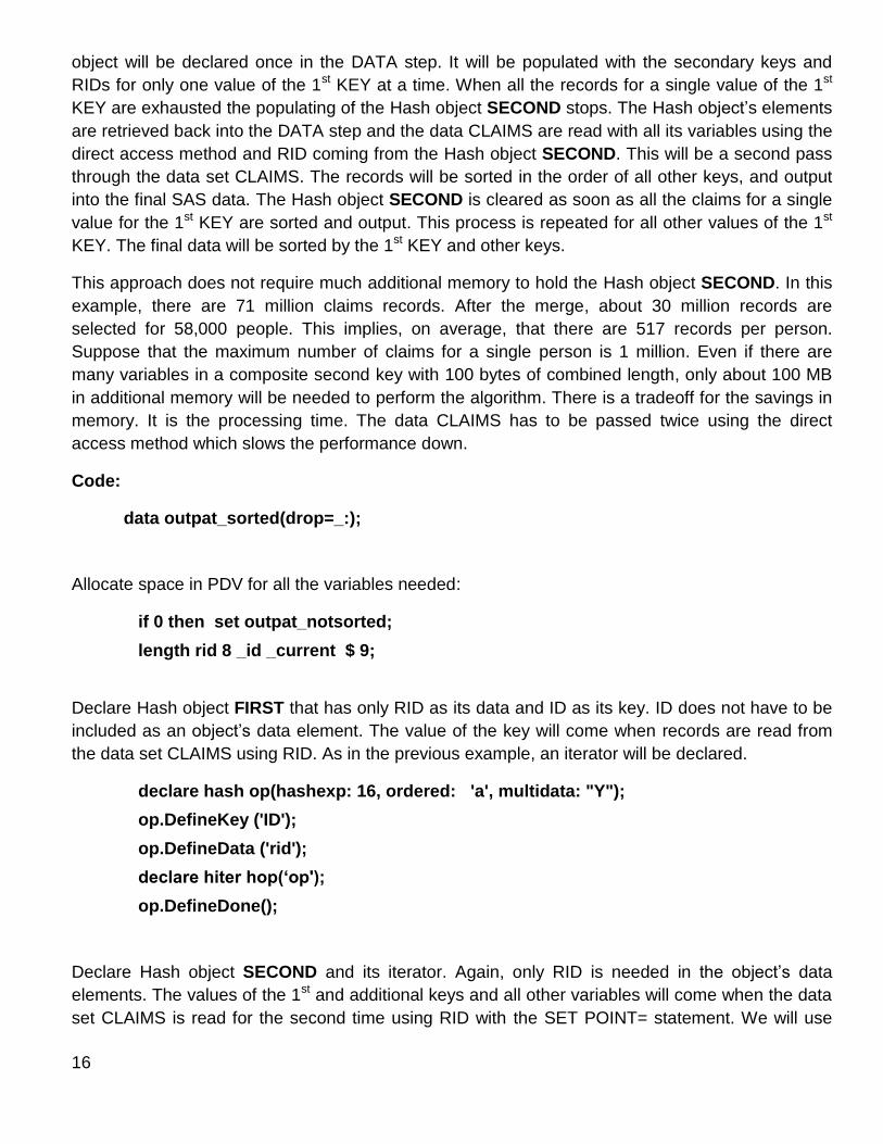
This approach does not require much additional memory to hold the Hash object SECOND. In this
example, there are 71 million claims records. After the merge, about 30 million records are
selected for 58,000 people. This implies, on average, that there are 517 records per person.
Suppose that the maximum number of claims for a single person is 1 million. Even if there are
many variables in a composite second key with 100 bytes of combined length, only about 100 MB
in additional memory will be needed to perform the algorithm. There is a tradeoff for the savings in
memory. It is the processing time. The data CLAIMS has to be passed twice using the direct
access method which slows the performance down.
Code:
data outpat_sorted(drop=_:);
Allocate space in PDV for all the variables needed:
if 0 then set outpat_notsorted;
length rid 8 _id _current $ 9;
Declare Hash object FIRST that has only RID as its data and ID as its key. ID does not have to be
included as an object’s data element. The value of the key will come when records are read from
the data set CLAIMS using RID. As in the previous example, an iterator will be declared.
declare hash op(hashexp: 16, ordered: 'a', multidata: "Y");
op.DefineKey ('ID');
op.DefineData ('rid');
declare hiter hop(‘op');
op.DefineDone();
Declare Hash object SECOND and its iterator. Again, only RID is needed in the object’s data
elements. The values of the 1st and additional keys and all other variables will come when the data
set CLAIMS is read for the second time using RID with the SET POINT= statement. We will use

17
the second keys as object’s keys. We do not need the first key (ID) in the Hash object’s keys
because the value of ID is the same for every element of a particular instance of the object.
declare hash personop(hashexp: 16,
ordered: 'a', multidata: "Y");
personop.definekey(‘SRVC_BGN_DT', ‘SRVC_END_DT');
personop.definedata('rid');
declare hiter hpersonop('personop');
personop.definedone();
drop rid rid_save SRV_BGN_DT_save SRV_END_DT_save ;
Load Hash Object FIRST keeping 1st KEY and RID only:
do rid=1 by 1 until (EndOfData);
set outpat_notsorted( keep=ID) end=EndOfData;
op.add();
end;
Read the Hash object FIRST back into the DATA step and retrieve 1st KEY and additional keys
(SRVC_BGN_DT SRVC_END_DT) from data CLAIMS in the order as they appear in the Hash
object FIRST using RID. Rename the 1st KEY so that track can be kept of whether the claims are
still being read for the same value of the 1st KEY. A variable _current is used to keep the value of
the 1st KEY from the previous record. It is set to “ “ in the beginning. A comparison of _current and
_id will determine whether the claims for the same value of the 1st KEY are being processed or a
new claim for the next value of the 1st KEY is being read. When _current=’ ‘, it means that the first
claim for the first value of the 1st KEY is being read.
do _iorc_=hop.first() by 0 while (_iorc_=0);
set outpat_notsorted(rename=ID=_id
keep=id SRVC_BGN_DT SRVC_END_DT) point=rid;
If the value of the 1st KEY (ID) is still the same, continue populating the Hash object SECOND. If
the 1st record for the next value of the 1st KEY is read, use the new variables rid_save,
SRV_BGN_DT_save and SRV_END_DT_save to save the values of RID and all the secondary
keys from that claim. The Hash object SECOND is not populated any further. The records from the
original data CLAIMS are retrieved a second time (this time with all the variables in CLAIMS) in the
order of the additional keys using RID from the Hash Object SECOND. These records are output
into the final SAS data:

18
if _id=_current or _current=" " then personop.add();
else do;
Save the current values for all keys and RID:
rid_save=rid;
SRV_BGN_DT_save=SRV_BGN_DT;
SRV_END_DT_save=SRV_END_DT;
do _iorcp_=hpersonop.first() by 0 while (_iorcp_=0);
set outpat_notsorted point=rid ;
output;
_iorcp_=hpersonop.next();
end;
Clear the Hash object SECOND:
personop.clear();
Restore the values for all keys and RID and populate the first element of the Hash object SECOND
with the values of additional keys (as keys) and RID (as data elements):
rid=rid_save;
SRV_BGN_DT=SRV_BGN_DT_save;
SRV_END_DT=SRV_END_DT_save;
personop.add();
end;
Save the value of the 1st KEY from the first pass through the data set CLAIMS into _current::
_current=_id;
Get the next element from the Hash object FIRST:
_iorc_=hop.next();

19
When the end of the Hash object FIRST is reached the process needs to be repeated (records for
the last value of the 1st key are still required sorting by the additional keys).
if _iorc_>0 then do;
do _iorcp_=hpersonop.first() by 0 while(_iorcp_=0);
set outpatclaims_notsorted point=rid ;
output;
_iorcp_=hpersonop.next();
end;
end;
end; /* End of loop reading from the Hash object FIRST (OP) */
run;
40*71 million = 2.8 GB of extra memory is needed for the Hash object FIRST plus 24*58,000 = 139
KB for the Hash object SECOND for the sort and merge. In comparison 56*71 million = 4 GB of
memory is required for a merge performed using a single Hash object. The difference in memory
will increase if there are more variables to sort the data by and more records in data CLAIMS. If all
the keys occupy 100MB, 140*71 million = 10GB of memory is needed for the single Hash object
approach compared to 2.8 GB for the “Hash of Hashes” approach. The saving in memory will result
in longer run time because of the two passes through the data set CLAIMS with the direct access
instead of one. This is a tradeoff worth considering.
Performance: with a merge
real time 1:06:37.37
user cpu time 6:15.65
system cpu time 48:39.17
memory 3164036.87k (3 GB)
5. Binary search implemented within the DATA step plus the direct access
method are used to select the desired records from the data CLAIMS
Although Paul Dorfman’s paper on lookup/search techniques had a different focus [5], a binary
search can be implemented in a SAS DATA step providing a useful algorithm. His article had the
code for binary search implementation, which is demonstrated in this paper. A greater performance
can be achieved by using binary search with Temporary Arrays because the search would be
implemented in memory. But more memory is needed to store data People in the array. The
algorithm below needs neither extra memory nor extra work disk space.

20
Suppose a small SAS data set, DATA2, with a key variable called ID2 is available as well as a big
SAS data set, DATA1, with a key variable called ID1. For each value of a key ID1, we want to
determine if it exists in DATA2.
The search process is organized as follows. We first divide the total number of records in a SAS
data DATA2 in half and compare the value of ID1 with the value of ID2 for that record. If the value
of ID1 is greater than the value of ID2 then we divide the second part of SAS data in half and
retrieve the value of ID2 for the record with a number (N+N/2)/2. Otherwise ID2 from a record with
a number of (1+N/2)/2 is retrieved. The process is repeated until the match is found or until there
are no records in between the last two comparisons.
For this algorithm to work, we need to have DATA2 sorted by the key variable ID2. This means that
we need to search for each values of the KEY from the data CLAIMS in data PEOPLE. The
resulting data will be merged but not be sorted. It could be much easier to sort it if we reduced the
number of the claims significantly after the merge. We do not need any extra work disk space or
any extra memory to perform the binary search.
Code:
data outpatclaims_selected(drop = _:) ;
set outpatclaims_notsorted;
_l = 1 ;
_h = n ;
do until ( _l > _h or _found ) ;
p = floor ((_l + _h) * 0.5) ;
set people (rename = (ID = _id)) point = p nobs = n ;
if ID< _id then _h = p - 1 ;
else if ID> _id then _l = p + 1 ;
else _found = 1 ;
end ;
if _found ;
run ;
If 58,000 choices are available (the size of data PEOPLE) only log2 (58,000) =17 passes to find
the match are needed. This means that if each value of the key of data CLAIMS that has 71 million
records is searched for, the direct access method is used 17* 71 million=1,207 million times.
Let us suppose the data CLAIMS is sorted. The algorithms could be reversed. In other words, the
search on IDs in data CLAIMS for every value of the key in data PEOPLE can be performed. Only
log2 (71 million)= 27 passes for each search key and 27*58,000=1,566,000 direct reads from the
data are needed. This algorithm could become more efficient than the DATA step merge after

21
sorting the data. But the program will become more complex because one- to-many merge has to
be implemented which the code above does not do.
Performance: merge without sorting
real time 43:11.42
user cpu time 17:41.18
system cpu time 25:06.43
memory 940.40k
PROC FORMAT was more efficient because of in-memory processing comparing to the binary
search using the direct access method.
SUMMARY TABLE:
The table below summarizes the use of resources for all methods described in the paper.
Method Disk Work Space Processing
(R.T.,CPU)
Memory
Sort and Merge -
with options
3-4 times of size of data. 42m/14m
70h/2h28m
small amount
PROC SQL, sorting
by all Keys
Needs more resources
than sort and merge
21m / 9m small amount
Using Indexes
When on disk
When in memory
No extra disk space
needed
1h30m/1h30m
3m/3m30s
Not needed
Allocated 130G-100G
not sufficient. Needs
more space than size
of data.
Merge using
Formats
(no sorting)
no additional space
needed
1h32m / 6.5m Small amount: loads
small data into memory
(8 MB)
RID and PROC
SORT and Merge
(single Key)
3-4 times the size of small
data with RID and Keys
(~12GB)
43m / 39m small amount
RID and Hash
object: Sort and
Merge by all KEYs
No additional disk space is
needed
47m / 37m Size of the small data
with Keys and RID
into HASH (4 GB)

22
RID and two Hash
objects
Hash of Hashes
No additional disk space
is needed
1h6m / 55m
Direct Access 2
times
Space as above plus
space for SECOND
HASH (2.8GB +
100MB?)
Binary Search
(Merge no Sorting)
No additional disk space
is needed
43m / 43m No additional memory
needed
CONCLUSIONS:
This paper presents several methods for working with large data in a setting where programmers
are competing for computer resources. The key lessons are:
1. Hash Objects combined with the direct access method and RID (Record Identifier) add
flexibility to programming tasks that require significant amount of disk work space. They
make the tasks feasible. You can benefit also from very fast in-memory algorithms.
2. Knowing the trade-offs of selecting a technique is important for designing efficient programs
in the competing environment for different computer resources.
3. Creating Indexes and loading the whole data into memory might be a very simple and
efficient solution if there is enough memory to load the data.
REFERENCES:
[1] “Hash + Point + Key” Paul M. Dorfman, NESUG 2011
[2] “Programming Techniques for Optimizing SAS Throughout” Steve Ruegsegger, NESUG
2011
[3] “Creating and Exploiting SAS Indexes” Michael A. Rathel, SUGI 29
[4] “Building Provider Panels: An Application for the Hash of Hashes” Judy Loren, NESUG
2011
[5.] “Array Lookup Techniques: From Sequential Search To Key Indexing
(Part 1)”, Paul M. Dorfman, NESUG 1999.
[6] “Hashing: Generations”, Paul M. Dorfman, Greg Snell, SUGI 28
[7] “Quick & Simple Tips”,Kirk Paul Lafler, Software Intelligence Corporation,
http://www.sconsig.com/sastips/using_the_proc_sql_method_option.pdf
[8] “SQL Joins -- The Long and The Short of It”, Paul Kent, SAS Institute
Inc., http://support.sas.com/techsup/technote/ts553.html

23
If you are not familiar with the Hash objects but are inspired by this paper read:
“I cut my processing time by 90% using hash tables - You can do it too!”Jennifer K. Warner-
Freeman, PJM® Interconnection, Norristown, PA. ,
“Getting Started with the DATA Step Hash Object” Jason Secosky & Janice Bloom – SAS Institute
Inc., Cary, NC
Various articles by Paul Dorfman on the Hash objects
ACKNOWLEDGMENTS
SAS and all other SAS Institute Inc. product or service names are registered trademarks or
trademarks of SAS Institute Inc. in the USA and other countries. ® indicates USA registration.
Other brand and product names are trademarks of their respective companies.
I would like to thank Paul Dorfman for his help on this paper, as well as my two supervisors,
Sharon-Lise Normand and Nancy Keating, who have supported me on this paper, Vanessa Azzone
for her editing help, and BASUG SC members who encouraged me to write the paper. I am also
indebted to my husband who does not know anything about SAS and programming, but
nonetheless, read the paper many times to provide editorial comments, and who walked the dog
and prepared multiple dinners while I worked on the paper.
CONTACT INFORMATION
Your comments and questions are valued and encouraged. Contact the author at:
Rita Volya
Department of Health Care Policy
Harvard Medical School
180 Longwood Ave
Boston, MA 02115
(617) 432-4476