Alternating Direction Optimization for Imaging Inverse ...plc/figueiredo2012.pdf · Alternating...
44
1 LJLL, Paris, 2012 Alternating Direction Optimization for Imaging Inverse Problems and Machine Learning Mário A. T. Figueiredo Instituto Superior Técnico, and Instituto de Telecomunicações Technical University of Lisbon PORTUGAL [email protected], www.lx.it.pt/~mtf
Transcript of Alternating Direction Optimization for Imaging Inverse ...plc/figueiredo2012.pdf · Alternating...

1 LJLL, Paris, 2012
Alternating Direction Optimization
for Imaging Inverse Problems
and Machine Learning
Mário A. T. Figueiredo
Instituto Superior Técnico, and Instituto de Telecomunicações
Technical University of Lisbon
PORTUGAL
[email protected], www.lx.it.pt/~mtf

2 LJLL, Paris, 2012
Outline
1. Review of optimization formulations for inverse problems
2. Iterative shrinkage and its accelerated variants
3. Alternating direction optimization: General formulation
4. Linear-Gaussian observations: the SALSA algorithm.
5. Deblurring Poissonian images: the PIDAL algorithm
6. Other topics: non-periodic deconvolution
hyperspectral unminxing,
group regularization,
hybrid synthesis-analysis formulations

3 LJLL, Paris, 2012
Inference/Learning via Optimization
Many inference criteria (in signal processing, machine learning) have the form
regularization/penalty function, negative log-prior, …
… typically convex, maybe non-differentiable (to induce sparsity)
Examples: signal/image restoration/reconstruction, sparse representations,
compressive sensing/imaging, linear regression, logistic
regression, channel sensing, support vector machines, ...
data fidelity, observation model, negative log-likelihood, loss,…
… usually smooth and convex.

4 LJLL, Paris, 2012
The Data Term
Examples:
Signal reconstruction (e.g., deconvolution) from linear-Gaussian observations,
linear regression:
f(x) =1
2kBx¡ yk22
Signal reconstruction (e.g., deconvolution) from linear-Poisson observations:
f(x) =
mX
i=1
»((Bx)i; yi);
yi 2 N0
=1
2
mX
i=1
¡(Bx)i ¡ yi
¢2
Logistic regression; training data , , (z1; y1); :::; (zN ; yN)
f(x) =
NX
i=1
³hzi;xyii ¡ log
KX
y0=1
exphzi;xy0i´
yi 2 f1; :::;Kg

5 LJLL, Paris, 2012
A Dichotomy: Unconstrained Versus Constrained
x̂ 2 argminx
f(x) + ¿c(x)
Unconstrained optimization formulation
Constrained optimization formulations
(Morozov regularization)
All “equivalent”, under mild conditions; often not equally convenient/easy.
(Ivanov regularization)
(Tikhonov regularization)

6 LJLL, Paris, 2012
Another Dichotomy: Analysis vs Synthesis
proper, closed, convex (not strictly), and coercive.
typical (sparseness-inducing) regularizer
e.g. , where is the observation operator
is a synthesis operator (e.g., of a Parseval frame )
[Elad, Milanfar, Rubinstein, 2007], [Selesnick, F, 2010],
Frame-based “synthesis” regularization
contains representation coefficients (not the signal/image itself)
f(x) = L(Ax)
x̂ 2 argminx
f(x) + ¿c(x)

7 LJLL, Paris, 2012
proper, closed, convex (not strictly), and coercive.
typical frame-based analysis regularizer:
A Fundamental Dichotomy: Analysis vs Synthesis
TV is also “analysis”; proper, lsc, convex (not strictly), but not coercive.
analysis operator (e.g., of a Parseval frame, )
x̂ 2 argminx
f(x) + ¿c(x)
Frame-based “analysis” regularization
is the signal/image itself, is the observation operator
c(x) = Á(Px)

8
Iterative Shrinkage/Thresholding (IST) or Proximal Gradient
The Moreau proximity operator [Moreau 62], [Combettes 01], [Combettes, Wajs, 05].
IST algorithm [F and Nowak, 01, 03],
[Daubechies, Defrise, De Mol, 02, 04],
[Combettes and Wajs, 03, 05],
[Starck, Candés, Nguyen, Murtagh, 03],
Forward-backward splitting [Bruck, 1977], [Passty, 1979], [Lions and Mercier, 1979],
Classical cases: c(z) =1
2kzk22 ) prox¿c(u) =
u
1 + ¿
u
soft(u; ¿)

9 LJLL, Paris, 2012
Key condition in convergence proofs: is Lipschtz
…not true with Poisson or multiplicative noise.
Difficulties with Iterative Shrinkage/Thresholding (IST)
…IST is known to be slow when is ill-conditioned and/or when is very small. B
Even for the linear/Gaussian case f(x) =1
2kBx¡ yk2
Accelerated versions of IST: Two-step IST (TwIST) [Bioucas-Dias, F, 07]
Fast IST (FISTA) [Beck, Teboulle, 09], [Tseng, 08]
Continuation [Hale, Yin, Zhang, 07], [Wright, Nowak, F, 09]
SpaRSA [Wright, Nowak, F, 08, 09]
others…

10
Unconstrained (convex) optimization problem:
Equivalent constrained problem:
s.t. Gz¡u= 0Augmented Lagrangian (AL):
AL method, or method of multipliers (MM) [Hestenes, Powell, 1969]
equivalent
Alternating Direction Method of Multipliers (ADMM)

11
Alternating Direction Method of Multipliers (ADMM)
AL method, or method of multipliers (MM) [Hestenes, Powell, 1969]
Unconstrained (convex) optimization problem:
…maybe hard to jointly solve for (zk+1;uk+1)
ADMM [Glowinski, Marrocco, 75], [Gabay, Mercier, 76]
non-linear
Block-Gauss-Seidel
(NLBGS) step

12
Unconstrained (convex) optimization problem:
ADMM [Glowinski, Marrocco, 75], [Gabay, Mercier, 76]
Several interpretations: variable splitting + augmented Lagrangian + NLBGS;
Douglas-Rachford splitting on the dual [Eckstein, Bertsekas, 92];
split-Bregman approach [Goldstein, Osher, 08]
Alternating Direction Method of Multipliers (ADMM)
Many recent applications in machine learning and signal processing [Tomioka et al, 09], [Boyd et al, 11], [Goldfarb et al, 10], [Fessler et al, 11], [Mota et al, 10], ...

13 LJLL, Paris, 2012
Convergence of ADMM [Eckstein, Bertsekas, 1992]
Consider the problem
Let and be closed, proper, and convex and have full column rank.
The theorem also allows for inexact minimizations, as long as the
errors are absolutely summable.
limk!1
zk = ¹z
Let be the sequence produced by ADMM, with
then, if the problem has a solution, say , then
14 LJLL, Paris, 2012
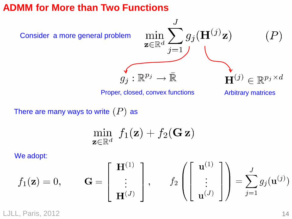
ADMM for More than Two Functions
Consider a more general problem
Proper, closed, convex functions Arbitrary matrices
We adopt:
There are many ways to write as

15 LJLL, Paris, 2012
Applying ADMM to More Than Two Functions
d(1)
k+1 = d(1)
k ¡ (H(1)zk+1 ¡u(1)k+1)
d(J)
k+1 = d(J)
k ¡ (H(J)zk+1 ¡u(J)k+1)
[F, Bioucas-Dias, 09], [Setzer, Steidl, Teuber, 09], [Combettes, Pesquet, 10, 11] (SDMM)
zk+1 =
· JX
j=1
(H(j))TH(j)
¸¡1µ JX
j=1
(H(j))T³u(j)
k + d(j)
k
´

16 LJLL, Paris, 2012
Applying ADMM to More Than Two Functions
zk+1 =
· JX
j=1
(H(j))¤H(j)
¸¡1µ JX
j=1
(H(j))T³u(j)
k + d(j)
k
´
Conditions for easy applicability:
inexpensive matrix inversion
u(J)
k+1 = proxg1=¹(H(J)zk+1 ¡d(j)k )
inexpensive proximity operators
u(1)
k+1 = proxg1=¹(H(1)zk+1 ¡d(j)k )

17 LJLL, Paris, 2012
Linear/Gaussian Observations: Frame-Based Analysis
Problem:
Template:
Convergence conditions: and are closed, proper, and convex.
has full column rank.
Mapping: ,
Resulting algorithm: SALSA
(split augmented Lagrangian shrinkage algorithm) [Afonso, Bioucas-Dias, F, 2009, 2010]

18 LJLL, Paris, 2012
Key steps of SALSA (both for analysis and synthesis):
Moreau proximity operator of
Moreau proximity operator of
ADMM for the Linear/Gaussian Problem: SALSA
Linear step (next slide):
zk+1 =
·A¤A+P¤P
¸¡1µA¤
³u(1)
k + d(1)
k
´+P¤
³u(2)
k + d(2)
k
´

19 LJLL, Paris, 2012
Handling the Matrix Inversion: Frame-Based Analysis
£A¤A+P¤P
¤¡1=£A¤A+ I
¤¡1Frame-based analysis:
Parseval frame
Compressive imaging (MRI):
subsampling matrix:
Inpainting (recovery of lost pixels):
subsampling matrix: is diagonal
is a diagonal inversion
matrix
inversion
lemma
Periodic deconvolution:
DFT (FFT) diagonal

20 LJLL, Paris, 2012
SALSA for Frame-Based Synthesis
Problem:
Convergence conditions: and are closed, proper, and convex.
has full column rank.
Mapping: ,
Template: A=BW
synthesis matrix
observation matrix

21 LJLL, Paris, 2012
Handling the Matrix Inversion: Frame-Based Synthesis
Frame-based analysis:
Compressive imaging (MRI):
subsampling matrix:
Inpainting (recovery of lost pixels):
subsampling matrix:
diagonal matrix Periodic deconvolution:
DFT
matrix inversion lemma +

22 LJLL, Paris, 2012
SALSA Experiments
9x9 uniform blur, 40dB BSNR
blurred restored
undecimated Haar wavelets, synthesis regularization.
23 LJLL, Paris, 2012
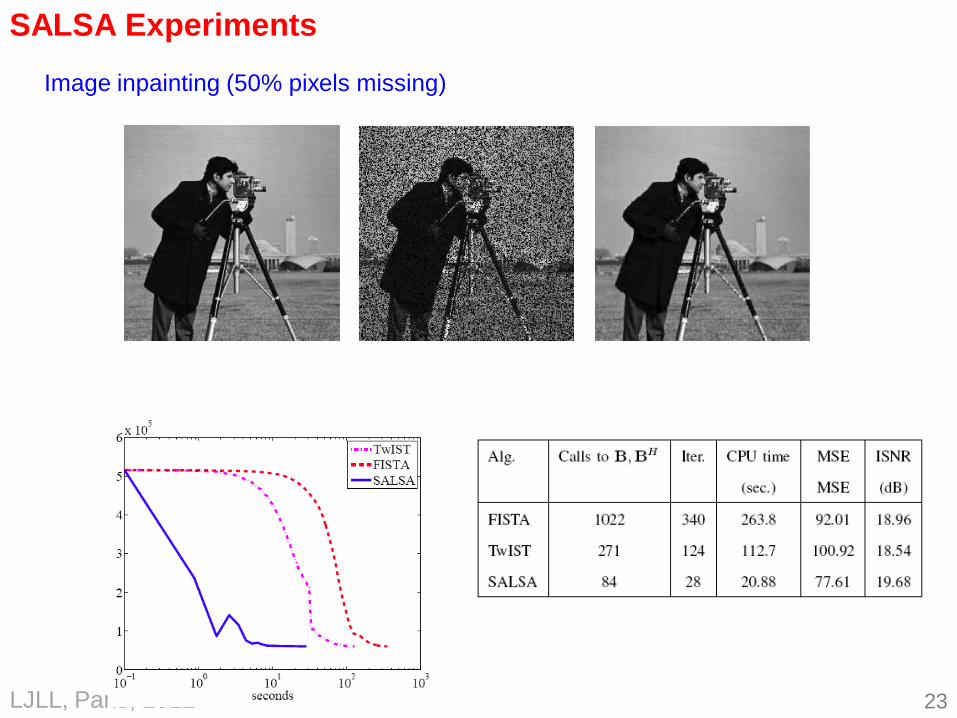
SALSA Experiments
Image inpainting (50% pixels missing)

24 LJLL, Paris, 2012
Frame-analysis regularization:
Frame-Based Analysis Deconvolution of Poissonian Images
Problem template:
Convergence conditions: , , and are closed, proper, and convex.
has full column rank
Same form as with:
hB¤B+P¤P+ I
i¡1=hB¤B+2 I
i¡1Required inversion:
…again, easy in periodic deconvolution, MRI, inpainting, …
positivity
constraint

25 LJLL, Paris, 2012
Proximity Operator of the Poisson Log-Likelihood
Proximity operator of the Poisson log-likelihood
Separable problem with closed-form (non-negative) solution
[Combettes, Pesquet, 09, 11]:
Proximity operator of is simply

26 LJLL, Paris, 2012
PIDAL Experiments
Comparison with [Dupé, Fadili, Starck, 09] and [Starck, Bijaoui, Murtagh, 95]
[Dupé, Fadili, Starck, 09] [Starck et al, 95]

27 LJLL, Paris, 2012
Morozov Formulation
Unconstrained optimization formulation:
Constrained optimization formulation:
basis pursuit denoising (BPN)
[Chen, Donoho, Saunders, 1998]
Both analysis and synthesis can be used:
frame-based analysis,
frame-based synthesis

28 LJLL, Paris, 2012
Constrained problem:
Proposed Approach for Constrained Formulation
…can be written as
Resulting algorithm: C-SALSA (constrained-SALSA)
[Afonso, Bioucas-Dias, F, 2010,2011]
full column rank
…which has the form
with

29 LJLL, Paris, 2012
Some Aspects of C-SALSA
Moreau proximity operator of is simply a projection on an ball:
As SALSA, also C-SALSA involves inversion of the form
·W¤B¤BW+ I
¸¡1or
·B¤B+P¤P
¸¡1
…all the same tricks as above.

30 LJLL, Paris, 2012
C-SALSA Experiments: Image Deblurring
Image deconvolution benchmark problems:
Frame-synthesis
Frame-analysis
Total-variation
NESTA: [Becker, Bobin, Candès, 2011]
SPGL1: [van den Berg, Friedlander, 2009]

31 LJLL, Paris, 2012
Handling Non-Periodic Deconvolution
x̂ 2 argminx
1
2kAx¡ yk22 + ¿c(x)
ADMM / SALSA handles this “easily” if is circulant (periodic convolution)
Analysis formulation for deconvolution
A
Periodicity is an
artificial assumption
A is (block) circulant
…as are other boundary conditions (BC)
Neumann BC Dirichlet BC
A is (block) Toeplitz A is (block) Toeplitz + Hankel
[Ng, Chan, Tang, 1999]

32 LJLL, Paris, 2012
Handling Non-Periodic Deconvolution
A natural BC: unknown values [Chan, Yip, Park, 2005], [Almeida, F, 2012]
unknown values
convolution, arbitrary BC masking
x̂ 2 argminx
1
2kMBx¡ yk22 + ¿c(x)
mask periodic convolution

33 LJLL, Paris, 2012
Handling Non-Periodic Deconvolution (Frame-Analysis)
Template:
x̂ 2 argminx
1
2kMBx¡ yk22 + ¿kPxk1Problem:
Naïve mapping: ,
H(2) = P;H(1) =MB
Better choice: g1(z) =1
2kMz¡ yk22; H(1) =B
·B¤B+P¤P
¸¡1=
·B¤B+ I
¸¡1Easy via FFT (periodic convolution)
proxg2=¹(u) = argminz
1
2¹kMz¡ yk22 +
1
2kz¡uk22
=¡MTM+¹I
¢¡1¡MTy+¹u
¢diagonal

34 LJLL, Paris, 2012
Non-Periodic Deconvolution: Example
9x9 uniform blur,
40dB BSNR
BC: replicate the boundary
rows/columns
Assuming periodic BC With edge tapering
Proposed method Periodic convolution
and deconvolution

35 LJLL, Paris, 2012
Another Application: Spectral Unmixing [Bioucas-Dias, F, 2010]
Goal: find the relative abundance of each “material” in each pixel.
Given library
of spectra
Indicator of the canonical simplex

36 LJLL, Paris, 2012
Spectral Unmixing
Problem:
Template:
Mapping: ,
Proximity operators are trivial.
Matrix inversion:
…can be precomputed; typical sizes 200~300 x 500~1000

37 LJLL, Paris, 2012
Yet Another Application: (Overlapping) Group Regularizers
minx2Rn
1
2kAx¡ yk22 +
kX
i=1
¸i Ái(xGi)
Groups (may overlap)
Gi µ f1; :::; ngFor groups with a hierarchical structure, and the or norm,
may still “computable” [Jenatton, Audibert, Bach, 2009] proxPiÁi
Ái `1; `2; `1
For arbitrary groups and norms, can be solved (FoGLASSO)
[Lui and Ye, 2010] (SLEP) `2 proxP
iÁi
It’s trivial to apply ADMM, as long as the are “simple” (next slide)
[F, Bioucas-Dias, 2011]
proxÁi
Alternative: re-write and use IST/FISTA
[Argyriou, Micchelli, Pontil, Shen, Xu, 2011]
kX
i=1
¸i Ái(xGi) = !(Cx)

38 LJLL, Paris, 2012
minx2Rn
1
2kAx¡ yk22 +
kX
i=1
¸i Ái(xGi)
(Overlapping) Group Regularizers
Problem:
Template:
Mapping: , J = k+1 gk+1(z) =1
2kz¡ yk22; gi(z) = ¸iÁi
H(k+1) =A;
minz2Rn
JX
j=1
gj(H(j)z)
H(i) = diag(I12Gi; :::; In2Gi
)
(binary diagonal)
h JX
j=1
(H(j))¤H(j)i¡1
=hA¤A+diag(jfGj : 1 2 Gjgj; :::; jfGj : n 2 Gjgj
i¡1Matrix inversion required:
Can be made proportional to identity,
without changing the objective function.

39 LJLL, Paris, 2012
(Overlapping) Group Regularizers
Toy Example: n = 200; A 2 R100£200 (i.i.d.N(0;1))
Ái = k ¢ k2; k = 19; G1 = f1; ::;20g; G2 = f11; :::;30g; :::
y =Ax+n; n »N(0;10¡2)
0 0.05 0.1 0.15 0.210
0
101
102
103
104
CPU time
Objective function
ADMM
FoGLASSO
0 0.05 0.1 0.15 0.210
-8
10-6
10-4
10-2
100
CPU time
MSE
ADMM
FoGLASSO

40 LJLL, Paris, 2012
Hybrid: Analysis + Synthesis Regularization
Observation matrix synthesis matrix
of a Parseval frame
As in frame-based “synthesis” regularization,
contains representation coefficients (not the signal itself)
these coefficients are under regularization
As in frame-based “analysis” regularization,
the signal is “analyzed”:
the result of the analysis is under regularization
analysis matrix of
another Parseval frame

41 LJLL, Paris, 2012
Problem:
Template:
Convergence conditions: all are closed, proper, and convex.
has full column rank.
Hybrid: Analysis + Synthesis Regularization
Mapping: ,

42 LJLL, Paris, 2012
Experiments: Image Deconvolution
Benchmark experiments:
Exp. Analysis
ISNR
Synthesis
ISNR
Hybrid
ISNR
Analysis
time (sec)
Synthesis
time (sec)
Hybrid
time (sec)
1 8.52 dB 7.13 dB 8.61 dB 34.1 4.1 11.1
2A 5.38 dB 4.49 dB 5.48 dB 21.3 1.4 3.8
2B 5.27 dB 4.48 dB 5.39 dB 20.2 1.6 3.4
3A 7.33 dB 6.32 dB 7.46 dB 17.9 1.6 3.7
3B 4.93 dB 4.37 dB 5.31 dB 20.1 2.5 3.9
Preliminary conclusions: analysis is better than synthesis
hybrid is slightly better than analysis
hybrid is faster than analysis
Two different frames (undecimated Daubechies 2 and 6); hand-tuned parameters.

43 LJLL, Paris, 2012
Summary and Ongoing Work:
Ongoing/future work: non-convex problems (no guarantees):
• non-convex regularizers
• blind deconvolution
• unmixing/separation/factorization
Thanks!
• Alternating direction optimization (ADMM) is powerful and versatile.
• Main hurdle: need to solve a linear system (invert a matrix) in each iteration…
• …however, sometimes this can be exploited to our advantage.
• State of the art results in several image/signal reconstruction problems.
• Other recent work: MAP inference in graphical models via ADMM [Martins, F, Aguiar, Smith, Xing, ICML’2012]

44 LJLL, Paris, 2012
Some Publications
M. Figueiredo and J. Bioucas-Dias, “Restoration of Poissonian images using alternating
direction optimization”, IEEE Transactions on Image Processing, 2010.
J. Bioucas-Dias and M. Figueiredo, ““Multiplicative noise removal using variable splitting
and constrained optimization”, IEEE Transactions on Image Processing, 2010.
M. Afonso, J. Bioucas-Dias, M. Figueiredo, “An augmented Lagrangian approach to the
constrained optimization formulation of imaging inverse problems”, IEEE Transactions
on Image Processing, 2011.
M. Afonso, J. Bioucas-Dias, M. Figueiredo, “Fast image recovery using variable splitting
and constrained optimization”, IEEE Transactions on Image Processing, 2010.
M. Afonso, J. Bioucas-Dias, M. Figueiredo, “An augmented Lagrangian approach to
linear inverse problems with compound regularization”, IEEE International Conference
on Image Processing – ICIP’2010, Hong Kong, 2010.
A. Martins, M. Figueiredo, N. Smith, E. Xing, P. Aguiar, “An augmented Lagrangian approach to
constrained MAP inference", International Conference on Machine Learning - ICML'2011,
Bellevue, Washington, USA, 2011.
M. Figueiredo, J. Bioucas-Dias, “An Alternating Direction Algorithm for (Overlapping) Group
Regularization”, Workshop on Signal Processing with Adaptive Sparse Structured Representations –
SPARS’11, Edinburgh, UK, 2011.