1

ALPHANOMICS:

The Informational Underpinnings of Market

Efficiency

By

Charles M. C. Lee

and

Eric C. So*

* Charles M. C. Lee is the Joseph McDonald Professor of Accounting at the Stanford Graduate School of

Business. Eric So is the Sarofim Family Career Development Assistant Professor at Sloan School of

Management, Massachusetts Institute of Technology. We thank Charles McClure for comments and

suggestions. We also greatly appreciate the thoughtful input of Scott Richardson (Reviewer) and Stephen

Penman (Editor). Finally, a special thanks to Stefan Reichelstein for not allowing us to give up on the

project.

2

ALPHANOMICS:

The Informational Underpinnings of Market Efficiency

TABLE OF CONTENT

Volume I

Chapter 0 – Foreword

Chapter 1 – The Magic of Markets

Chapter 2 - Noise Trader Model

Chapter 3 – Equity Valuation

Volume II

Chapter 4 - Investor Sentiment

Chapter 5 - Limits to Arbitrage

Chapter 6 - Research Methodology Issues

3

FOREWORD

Assumptions matter. They confine the flexibility that we believe is available to us as

researchers, and they define the topics we deem worthy of study. Perhaps more insidiously,

once we’ve lived with them long enough, they can disappear entirely from our consciousness.

Mainstream accounting and economic thought is shaped by the assumptions of classical

information economics -- the study of normative behavior under full rationality assumptions.

While this powerful paradigm has proved highly instructive, it has also engendered an

unfortunate tendency for economists to attribute unlimited processing ability to decision makers.

We view this tendency as unfortunate, because it can inhibit the development of other potentially

promising avenues of research.

In the area of research into financial markets, the assumption of unbounded rationality has

produced a deep-seated faith in market efficiency that, for many years, detracted from potentially

fruitful inquiries along alternative paths. As economists, we tend to take for granted the efficacy

of the arbitrage mechanism, generally assuming that it involves few constraints, and little cost or

risk. Faith in the arbitrage mechanism has stunted the development of research in mainstream

economics on the dynamic process of information acquisition, analysis, and aggregation. Market

prices are often presumed to be correct, as if by fiat, and the process by which they become

correct is trivialized.

The depth of our collective faith in market efficiency is evident from our course offerings. At

most top business schools today, investment classes are taught by financial economists trained in

equilibrium thinking. In these classes, the efficient market hypothesis (EMH) is typically offered

as the intellectual high ground – an inevitable outcome of rational thinking. Students are taught

that market-clearing conditions require prices to reflect all currently available information. This

line of reasoning persists, despite the fact that it conforms neither to logic nor to evidence.

Why do we believe markets are efficient? Are these beliefs well-grounded? What are the

economic forces that keep markets efficient? How, when, and why might such forces fail? If we

choose to depart from the assumption of full efficiency, what alternatives do we have? Can we

4

do so without abandoning faith in individual rationality? And what might a sensible research

agenda look like for accounting and finance academics if markets were not fully efficient?

These are some of the questions we will explore in this monograph.

Implicitly or explicitly, each researcher working in the capital market area must come to terms

with these questions. The degree to which markets are efficient affects the demand for

accounting research in investment decisions, regulatory standard-setting decisions, performance

evaluations, corporate governance, contract design, executive compensation, and corporate

disclosure decisions. One’s belief about market efficiency also dictates our research design, and

in particular the role played by market prices in the analysis. Perhaps most importantly, given

the intended audience of this volume, one’s view about market efficiency will have a profound

effect on the shape of one’s research agenda. In fact, what a researcher chooses to study in the

capital market area is, we believe, largely a function of her level of faith in the informational

efficiency of these markets.

It has been 35 years since Michael Jensen famously proclaimed at a Journal of Financial

Economics (JFE) symposium: “I believe there is no other proposition in economics which has

more solid empirical evidence supporting it than the Efficient Market Hypothesis.” (Jensen

(1978, p95)). Less often quoted, but perhaps even more on the mark, were Jensen’s remarks at

the end of the same article. Commenting on the evidence presented at the symposium about

market pricing anomalies, he wrote: “I have little doubt that in the next several years we will

document further anomalies and begin to sort out and understand their causes. The result will

not be abandonment of the ‘efficiency’ concept, nor of asset pricing models. Five years from

now, however, we will, as a profession, have a much better understanding of these concepts than

we now possess, and we will have a much more fundamental understanding of the world around

us.” This monograph is an attempt to summarize what we have learned since, and what we as a

profession have to look forward to in the future.

As this is written, the winners of the 2013 Nobel Memorial Prize in Economics have just been

announced. This year the prize was shared by three Americans – Eugene Fama, Lars Peter

Hansen, and Robert Shiller. For many of us who have followed the EMH debate over the years,

5

the decision to honor Fama and Shiller together is not without irony, given the radical differences

in their views on the subject. Fama is being honored for his work in the 1960s showing that

market prices are accurate reflections of available information. Shiller is honored largely for

circumscribing that theory in the 1980s by showing that prices can deviate from rationality. In

awarding them the prize, the Royal Swedish Academy of Sciences notes that collectively the

three professors’ work “laid the foundation for the current understanding of asset prices.” In

characterizing this contribution, the committee said their findings “showed that markets were

moved by a mix of rational calculus and human behavior.”

Markets are moved by a mix of rational calculus and human behavior. We have certainly come

a long way since the days of the 1978 JFE symposium! As Jensen predicted, financial

economists have not abandoned rational calculus or the concept of ‘efficiency.’ We understand

and still appreciate the power of equilibrium thinking. At the same time, however, after 35

years, we have also come to acknowledge the importance of human behavior and arbitrage costs

in asset pricing. As a profession, many more of us are now willing to entertain, and wrestle with,

the limitations and problems of an imperfect market. In this sense, we have indeed come to a

much better place in terms of our understanding of the world around us.

In recent decades, the focus of academic research on market efficiency has gradually shifted

from the general to the more specific. While earlier studies tended to view the matter as a yes/no

debate, most recent studies now acknowledge the impossibility of fully efficient markets, and

have focused instead on factors that could materially affect the timely incorporation of

information. An extensive literature in finance has developed that examine the effect of “noise

trader demand”, or “investor sentiment” (broadly defined as price pressures of a non-

fundamental origin). As we cover in more detail in Chapters 2 and 4, there is now substantial

evidence that investor sentiment can affect asset pricing, as well as real economic decisions

(such as corporate finance, investments, dividend policies, and disclosure decisions).

At the same time, increasing attention is being paid to how regulatory and market design issues

could either impede or enhance market pricing efficiency through their effect on information

arbitrageurs. Recent evidence on the limits of arbitrage highlights the complexity and non-

6

monotonicity of the process through which prices converge towards fundamental value. To

better understand the relationship between prices and information flows, we need to gain a

deeper appreciation for how rational information arbitrage actually operates.

Whatever one’s view is of market efficiency, few scholars today deny the fact that active asset

management, with “beating the market” as its central mandate, is today a large and thriving

business. The reason our financial markets are even remotely efficient, is because sufficient

resources are being spent each day on keeping it so.1 The agents who acquire and process new

information aspire to making a profit from their investment. Their continued survival speaks

powerfully to magnitude of the aggregate mispricing in equilibrium. At the same time, these

purveyors of information face a complex production function, with multiple costs and risks,

including: time-varying capital constraints, moral hazard problems, risk management issues,

security lending costs, and various practical implementation challenges. This monograph, and in

particular, Chapter 5, will highlight some of these limits to arbitrage.

In short, our goal is to present and promote a more nuanced view of market efficiency. In our

view, a naïve form of efficiency, in which price is assumed to equal fundamental value, is a

grossly inadequate starting point for much of today’s market-related research.2 To us, this is an

over simplification that underweights the role of costly information and fails to capture the

richness of market pricing dynamics and the process of price discovery. Prices do not adjust to

fundamental value instantly by fiat. In reality market prices are buffeted by a continuous flow of

information, or rumors and innuendos disguised as information. Individuals reacting to these

signals, or pseudo-signals, cannot easily calibrate the extent to which their own signal is already

reflected in price. This noisy process of price discovery requires time and takes effort, and is

only achieved at substantial cost to society.

1 As discussed in more detail in Chapter 1, we estimate the amount of asset-under-management (AUM) controlled

by professional active managers to be at least $60 trillion USD as of the end of 2012. The U.S. mutual fund

market alone exceeds $6 trillion, and the hedge fund market is at least $2 trillion (See the 2013 Investment

Company Factbook, available at http://www.icifactbook.org/). Thus it clearly takes a great deal of capital and

resources to attain the level of pricing efficiency we currently enjoy. 2 Throughout this discourse, fundamental value is defined as the expected value of future dividends, conditional on

currently available information. See Chapter 1 for a more detailed definition of the efficient market hypothesis

(EMH).

7

When information processing is costly, research opportunities abound. Given noisy prices and

costly arbitrage, academic research can add value by improving the cost-effectiveness of the

arbitrage mechanism.3 Some of this research will lead to superior techniques for identifying

arbitrage opportunities. Other research will focus on sources of systematic noise, exploring

behavioral and non-fundamental reasons why prices might diverge from value. Still others, such

as work on earnings quality or fundamental analysis, will help to narrow the plausibility bounds

around the value estimates of traded securities.

Finally, research into arbitrage constraints and market design issues can help us to better

understand and manage the costs faced by those who seek to acquire information and make

markets more efficient. How might the incentives of these agents be affected by changes in

security market regulations and mandatory corporate disclosure rules (such as fair value

accounting or the adoption of IFRS)? How is the information acquisition and alpha extraction

process being impacted by Big Data? To us, a wide world of research opportunities opens up

once we are willing to lift the hood, and peer behind the assumption of market efficiency.

Much of this research has a utilitarian focus. It is decision driven, interdisciplinary, and

prospective in nature. It assumes a user, rather than a preparer, orientation towards accounting

information. It does not assume the market price is equivalent to fundamental value. Rather, it

produces independent estimates of firm value that may be used to challenge, and perhaps

discipline, prices. Its end goal is to improve the allocation of scarce resources through more cost-

effective usage of information in solving significant problems in financial economics.

This monograph is dedicated to the kind of decision-driven and prospectively-focused research

that is much needed in a market constantly seeking to become more efficient. We refer to this

type of research as “Alphanomics”, the informational economics behind market efficiency. The

“Alpha” portion refers to the abnormal returns, or financial rewards, which provide the incentive

for some subpopulation of investors to engage in information acquisition and costly arbitrage

3 We define arbitrage as information trading aimed at exploiting market imperfections. As discussed later, this

definition is broader than the definition found in some finance textbooks.

8

activities. The “Nomics” refers to the economics of alpha extraction, which encompasses the

costs and incentives of informational arbitrage as a sustainable business proposition.

We caution the reader on two caveats. First, the evidence we survey here focuses primarily on

equity securities, and in particular public equities listed in the U.S. We acknowledge that in

finance, an extensive literature explores related topics across multiple asset classes in a more

global setting. Although this literature is covered only tangentially by this volume, many of the

same principles discussed here apply across other asset classes. Second, we are focused on

market efficiency in an informational sense – i.e., whether and how prices incorporate available

information. Tobin (1984) entertains a broader definition of economic efficiency which we find

intriguing, particularly his views on the “functional efficiency” of free markets. For parsimony,

our monograph does not tread in that direction, but interested readers are encouraged to include

Professor Tobin in their list of must-read references.

This volume is itself interdisciplinary. The first two chapters in particular draw heavily from the

writings of financial economists. In Chapter 1, titled “The Magic of Markets,” we revisit the

theoretical foundations of the EMH, and discuss some of the limitations and biases it engenders.

Some have compared the EMH to “Newtonian physics” in the sense that while we know it does

not hold precisely, the theory is a safe operating assumption for practical purposes. We critically

evaluate this claim, and discuss situations where the EMH falls particularly short.

Chapter 2 introduces a simple Noise Trader Model (“NTM”) first featured in Shiller (1984). A

particularly appealing aspect of the NTM is its explicit recognition of the role played by

information costs. In contrast to the EMH, which assumes information costs are trivial, the role

for information arises endogenously in the NTM and the cost of information acquisition and

analysis has direct implications for equilibrium pricing.4

4 Noisy rational expectation models, such as Grossman (1976), Grossman and Stiglitz (1980), and Diamond and

Verrecchia (1981), also feature noise traders and other informed traders, who incur costs in order to become

informed. We discuss the most salient differences between the NTM and these models in Chapter 2.

9

Chapter 3 examines equity valuation. An independent estimate of firm value is needed if

information arbitrageurs are to challenge and discipline price. We discuss the role of historical

accounting information in the formulation of such an estimate. Specifically, we review the

fundamental economics that link historical financial statement numbers to a firm’s fundamental

value. Using the residual income model (RIM) as a framework, we integrate the investment

approaches advocated by such legendary investors as: Ben Graham, Warren Buffett, and Joel

Greenblatt. This analysis shows that the strategies espoused by these investors actually dovetail

nicely with the recent evidence from academic research on the predictability of stock returns.

Chapter 4 expands the discussion of Investor Sentiment. Financial economists have long

observed that stock prices seem to respond to price pressures that cannot be easily traced back to

fundamentals (e.g., Roll (1984), Black (1986), Cutler, Poterba, and Summers (1999)). In this

chapter, we survey the extensive literature on noise trading and investor sentiment that has

developed over the past three decades. We show that evidence in favor of a role for human

behavior and investor sentiment in asset pricing is now extensive. We also discuss the

implications of these findings for the future of accounting research.

Chapter 5 examines Limits to Arbitrage. In the NTM, the extent to which prices may wander

away from fundamentals is a function of the costs faced by informed arbitrageurs. Thus

reducing arbitrage costs will lead directly to greater pricing efficiency. We dissect the major

components of these costs using the concept of “asset substitutability,” and discuss how each

component might impact common investment strategies employed by hedge funds. We also

discuss academic studies that shed light on the cost constraints faced by arbitrageurs.

Chapter 6 focuses on Research Methodology. In this chapter, we review research design issues

for academics interested in working on questions related to market efficiency. Specifically, we

discuss techniques for distinguishing between whether a predictable pattern in prices is due to

risk or mispricing. We also speculate on future research directions in this area, using recent

studies as illustrations.

10

In sum, this monograph may be viewed as our attempt to reconcile the theory of market

efficiency, so popular among academics, with the practice of active investing, so prevalent in

industry. Active investing is big business, and it is rooted in the basic premise that the search for

information not yet reflected in prices can be a worthy pursuit. It is difficult to begin serious

academic analyses of this industry without an economic framework that anticipates the continued

existence of mispricing in equilibrium. We offer such a framework.

At the same time, we hope this monograph will serve as a conceptual bridge for future dialogue

between academics and financial practitioners. For academics, our hope is that this volume will

help you to better appreciate the perspective of active investors who make a living attempting to

beat the market. For financial practitioners, this is our attempt to provide a framework for

thinking about active investing as a science, and to bring together a volume of academic work

that may bear on your efforts to improve market efficiency.

We hope you enjoy the ride.

11

References

Tobin, J., 1984, On the efficiency of the financial system, Lloyds Bank Review, July, 1-15.

12

Chapter 1

The Magic of Markets

In this chapter, we trace the progression of economic thought on market efficiency.5 We discuss

what is meant by the efficient market hypothesis (EMH), and some of the most pressing

problems an undue reliance on market efficiency has engendered in the profession. Beginning

with Hayek (1934), we review the informational role of markets in free enterprise systems. We

then discuss the untenable case for perfectly efficient markets (Grossman and Stiglitz (1980))

and argue for a broader research agenda that recognizes the importance of the market for

information.

1.1 The Value of Markets in Society

In his justly famous treatise on the subject of knowledge aggregation in society, Hayek (1945)

contrasted centralized-planning with a market-based economy based on decentralized decision

making. Hayek noted that economic planning involves two types of knowledge: (1) scientific

knowledge (knowledge about theoretical or technical principles and rules), and (2) specific

knowledge (knowledge of particular circumstances of time and place). Recognizing that even the

best central planner does not have adequate access to knowledge of the second type, Hayek

argued that market-based economies in which resource allocation decisions are decentralized

will always dominate centralized planning. This is because in a rational economic order,

efficient social planning will always depend on “the utilization of knowledge not given to anyone

in its entirety” (p.520).

With the benefit of hindsight, the genius of Hayek is clear. After WWII, multiple country-level

paired-experiments emerged that offered a remarkable glimpse into the power of market-based

planning: North and South Korea; East and West Germany; Taiwan and Communist China. In

each case, holding constant cultural and genetic factors, decentralized economies dominated

centrally-planned ones. This dominance is seen not merely in terms of personal economic

wealth (i.e. per capita GDP). On almost every conceivable metric of social wellness (Education;

5 For other survey studies that cover overlapping themes, see Lee (2001), Richardson, Tuna, and Wysocki (2010),

Asness and Liew (2014), and Campbell (2014).

13

Opportunity; Nutrition and Healthcare; Life Expectancy; and Basic Human Needs), the market-

based systems dominated.6 As Margaret Thatcher, champion of the free market gospel, once

quipped: “capitalism is humanitarianism.” In short, markets work and there is little wonder that

the 20th

century has been called “the Hayek Century” (Cassidy (2000)).

But what gives the market economies their magic? It boils down to better resource allocation via

decentralized decision making. As Hayek observed, the essential planning problem of society

involves rapid adaptation to changing circumstances. It is an information game that the central

planner cannot hope to win. It follows then that “the man (woman) on the spot” is the best

person to make resource allocation decisions.7

What is the role of prices in all this? Consider what the “man (woman) on the spot” needs to

make resource allocation decisions. As a minimum, she needs to know the relative scarcity of

things – the value of the inputs and outputs relevant to her decision. This information is quickly

and succinctly summarized by prices. The pricing system is a vital knowledge aggregation

mechanism in free markets. To the extent that market prices are meaningful indicators of

relative scarcity, they help facilitate decentralized planning. Price, in short, is a public good that

is essential in enabling decentralized decision-making.

Given these basic tenets of free market economics, the efficiency with which market prices

assimilate new information assumes an importance beyond academic debates over the size of the

abnormal returns earned by hedge fund managers. If the prices of things drive decentralized

decisions and decentralized decision-making drives free enterprise systems, then prices play a

pivotal role in economic proliferation by revealing the value of scare resources. This is because

free enterprise economies depend on their markets to set prices, which in turn determine resource

allocation throughout the system.

6 A good resource for those interested in broad measures of social progress is: www.socialprogressimperative.org.

7 Hayek argued that due to this information game, planning must be decentralized. Government intervention in a

free market only serves to forestall economic ailments and could lead to political oppression. In the Road to

Serfdom, he warns ominously: “the unforeseen but inevitable consequences of socialist planning create a state of

affairs in which, if the policy is to be pursued, totalitarian forces will get the upper hand.”

14

We thus draw two key lessons from Hayek: (1) the informational role of markets in knowledge

aggregation is of great value to society, and (2) asset prices that reflect the value of goods (and

services) are central to the development of free market systems.

Notice, however, that neither Hayek, nor the broader Austrian school of economics to which he

belonged, was focused on the specifics of how markets become efficient, or when the knowledge

aggregation process might fail. These earlier works were focused on the central battle of their

day: whether market systems are better than centrally planned ones. They are largely silent with

respect to the economics of information acquisition and analysis, and the factors that might cause

markets to become more or less price efficient. These issues were not their primary concern.

The idea that markets serve as powerful aggregators of knowledge, first proposed by Hayek, has

in our day morphed into what we refer to as the EMH. In the next subsection we discuss why

this turn of events has led to some inevitable problems.

1.2 The Joint Equilibrium Problem

What is our main objection to the EMH? Let’s begin with what we do not object to. First, we

recognize that markets are wonderful aggregators of information. Second, like proponents of the

EMH, we appreciate the power of equilibrium thinking. Third, we acknowledge that not

everyone should be trying to beat the market. In fact, we concur with EMH proponents that most

individuals are better off assuming prices are reasonable indicators of the relative scarcity of

resources in society. All of these conclusions are consistent with Hayekian thinking.

Where we disagree with EMH proponents is in the assumption that the costs associated with

informational arbitrage are trivial or unimportant. Like Hayek, we believe the price discovery

and information aggregation process is central to the social value of markets. Some economists

today believe the EMH is the “moral high ground”, arguing that the existence of mispricing

necessarily implies off-equilibrium (non-economic or irrational) thinking. In fact, we believe the

exact opposite is true. In terms of equilibrium thinking, it is the EMH that is conceptually

flawed and intellectually untenable.

15

Statements regarding the efficiency of market prices must first recognize the existence of two

interrelated but distinct markets. In addition to the market for the assets themselves, if

information is costly, we will have a separate market for information about these assets.

Participants in this second market buy and sell information about the underlying assets. These

participants incur costs to ‘buy’ (i.e., acquire) information with the expectation that they can

‘sell’ (i.e., convey) the information to the market in exchange for direct fees, in the case of

research analysts, and/or trading profits, in the case of investors. Equilibrium requires both

markets to clear. In other words, supply must equal demand in both markets.

In discussing the impossibility of perfectly efficient markets, Grossman and Stiglitz (1980) make

the following observation:

We have argued that because information is costly, prices cannot perfectly

reflect the information which is available, since if it did, those who spend

resources to obtain it would receive no compensation. There is a fundamental

conflict between the efficiency with which markets spread information and the

incentives to acquire information. [p.405]

Their point is simple. When information costs are non-trivial, some amount of mispricing must

remain in equilibrium. This must be the case if informed traders are to be sufficiently

compensated. In other words, market clearing conditions in this joint equilibrium (when supply

equals demand in both markets) require asset prices to bear the marks of inefficiency.

Given the inextricable link between these two markets, focusing on either in isolation would be

foolhardy. If we focus solely on the asset market, for example, we will observe “pricing

anomalies”, whose roots lie in the market for information. These asset pricing aberrations can

only be understood in the context of supply and demand in the parallel market for information.

Larger mispricings will remain, for example, when the cost of acquiring and exploiting

information about a firm is higher. This might be the case if the company’s operations are more

complex, its accounting is more opaque, or if informational extraction costs, such as market

16

liquidity and short-selling costs (i.e., the costs of profitably exploiting value-relevant

information) are higher.8

Our point is that financial economists need to pay more attention to the costs and incentives in

the market for information. The reason most individuals in society can rely on market prices to

make their everyday decisions is because some individuals in society do not. While it might be

alright for most (even the vast majority of) individuals in society to assume “the price is right” –

that is, to free ride on the efforts of information arbitrageurs – economists that study how

markets operates should not be counted among them.

Most people can assume a car will run each time the key is turned, however the auto mechanic

cannot afford to do so. Likewise economists interested in the informational role of markets also

need to look under the hood. We believe it would be an abdication of responsibility not to.

1.3 What do we mean by market efficiency?

Stripped down to its core, the efficient market hypothesis (EMH) is the simple proposition that

market prices incorporate all available information. The original EMH literature is careful to

condition this statement on a particular set of available information (e.g., Fama (1965, 1970,

1991)). Different forms of the EMH (strong, semi-strong, and weak) are then defined in terms of

the rapidity and accuracy of price adjustment to news within different information sets. Early

applications of the EMH in accounting also acknowledged that the speed and accuracy of price

adjustment to new information is a continuous process, and does not occur instantaneously (e.g.,

Dyckman and Morse (1986; page 2)).

Most empirical tests of market efficiency have focused on the predictability of returns. The idea

is that if current market prices incorporate all available information, then future returns should be

largely unpredictable. Or, at least any patterns of predictability that we observe in future returns

should not be easily exploited after transaction costs. This version of the EMH is often evoked,

8 Blocher et al. (2013) provides an excellent example of the joint equilibrium problem in the context of short-selling

constraints. Empirically, Beneish et al. (2013) links this phenomenon to nine well-known pricing anomalies in the

equity market.

17

for example, in deriving equilibrium conditions in asset pricing models. It has been variously

referred to as the “competitively efficient markets” hypothesis (Rubinstein (2001)), or the “no

arbitrage condition”. An even more descriptive moniker, we think, is the “No Free Lunch”

assumption. Markets that are in equilibrium should rarely, if ever, offer a free lunch.

Tests of the “no free lunch” hypothesis run quickly into a serious challenge, which Fama (1970,

1991) famously refers to as the “joint hypothesis problem”.9 To make any statement about

market efficiency, we need to assert how the market should reflect information – in other words,

we need an equilibrium asset pricing model. For example, the Capital Asset Pricing Model

(CAPM) states that the expected return on any security is proportional to the risk of that security

as measured by its market Beta, and nothing else should matter. Suppose we find evidence

against the predictive power of Beta for cross-sectional returns. One possibility is the EMH

holds, but CAPM is a poor model of how investors set prices. Perhaps prices do reflect all

information, but there are other risk factors besides Beta that investors are being compensated for

bearing. Another possibility is that the CAPM is in fact how investors should set prices, but they

are failing at it because of some sort of behavioral error or bias. Yet a third possibility is that

both EMH and CAPM are wrong. It is difficult to sort out where the problem lies.

It has been argued that the joint hypothesis problem renders the EMH impossible to conclusively

reject (Fama (1970, 1991)). We agree that this problem limits what researchers can say about

market efficiency on the basis of return predictability alone. However, it does not leave us

paralyzed and powerless. We believe there are now multiple methods for evaluating the

reasonableness of a claim about market mispricing besides returns prediction. Some of these

involve examining ancillary evidence about firms’ future cash flows, operating profits, short-

window earnings announcement returns, analyst forecast revisions, probability of distress or

delisting, or short-sale activities, etc. Others studies (for example, Daniel and Titman (1997),

Hirshleifer et al. (2012) and Ohlson and Bilinski (2012)) rely on common sense “reasonableness”

tests to distinguish mispricing-based from risk-based explanations for returns predictability. The

main point being as researchers, we now have at our disposal a large set of holistic, “weight of

9 See Asness and Liew (2014) for a good discussion of the work by Fama and Shiller from the perspective of former

academics who are now active fund managers. Campbell (2014) provides a more academic review of their work.

18

evidence,” approaches that helps us to discriminate between risk and mispricing (this is the main

subject of Chapter 6; we also touch on it in this chapter, in Section 1.7.3).10

As difficult as it might be to disprove the “No Free Lunch” hypothesis, this version of the EMH

is not the main problem. As capital market research has evolved over time, a much stronger and

more insidious form of the EMH has gained currency. It is what we refer to as the “Price is

Right” hypothesis. Applied to equity markets, this view of market efficiency asserts that a

company’s stock price is an optimal forecast of the present value of its expected future dividends

(Pt = Vt, t). Notationally, this view is often expressed in the following form:

1 )1(

)(

ii

itt

tt

r

DEVP , (1)

where Vt is defined as the stock's fundamental value at time t, Et(Dt+i) is the expected future

dividend for period t+i based on information available at time t, and r is the appropriate risk-

adjusted discount rate for the expected dividend stream. Equation (1) asserts that Pt, the stock

price at time t, is equivalent to the expected value of future dividends, Vt.

Over time, the Price is Right view of markets has acquired the status of an operating assumption

among many researchers. For example, in the information content literature in accounting

(including both short-window event studies and long-window association studies), price is

commonly interpreted as a de facto proxy for the expected value of future dividends, and stock

returns are deemed to reflect changes in the present value of expected future dividends. In the

extensive value-relevance literature (Holthausen and Watts (2001) and Barth et al. (2001)), price

is deemed to be a normative benchmark for firm value. The assumption that price is equivalent

to the present value of expected future dividends appears more explicitly in valuation studies,

typically as the first assumption in the paper (e.g., Feltham and Ohlson (1999), Zhang (2000),

Dechow et al. (1999)).

10 Also see Richardson, Tuna, and Wysocki (2010) for a discussion of non-price based tests that can help

discriminate between risk and mispricing based explanations for returns predictability.

19

In finance, this assumption has become a cornerstone of empirical asset pricing, particularly

when interpreting realized returns. For example, highly influential work by Campbell (1991)

and Vouteenaho (2002) decompose realized returns under the assumption that movements in

stock prices mirror movements in Vt. In a zero-sum attribution exercise where price equals

value, what is not attributable to cash flows is, of necessity, attributed to discount rates. Thus,

due to an uncritical application of the EMH, the unexplained volatility in stock prices is now

widely interpreted in the empirical asset pricing literature as evidence of time-varying expected

returns.11

The problem is that “No Free Lunch” does not imply “The Price is Right”. In his seminal study

on the role of mass psychology in markets, Robert Shiller (1984) made the following

observation:

Returns on speculative assets are nearly unforecastable; this fact is the basis of the

most important argument in the oral tradition against a role for mass psychology in

speculative markets. One form of this argument claims that because real returns are

nearly unforecastable, the real prices of stocks is close to the intrinsic value, that is,

the present value with constant discount rate of optimally forecasted future real

dividends. This argument for the efficient market hypothesis represents one of the

most remarkable errors in the history of economic thought. It is remarkable in the

immediacy of its logical error and in the sweep and implications of its conclusion

(Shiller (1984), p.458-59)). [emphasis ours].

With a little thought, Shiller’s point becomes obvious. If price is equal to value at all times, then

indeed returns will be unforecastable. In other words, if the price is always right (“A”), then

11 Some may argue that equation (1) is itself too naïve, as it does not allow for time varying expected returns. In

our view, this argument is a red herring. Of course, equation (1) is predicated on the fact that we can derive an ex

ante estimate of the cost-of-capital (risk adjusted) appropriate for a firm’s risk level. It would make no sense

otherwise. However, irrespective of how a firm’s expected return varies over time, at any given point in time one

should be able to provide a point estimate for its expected return (a constant equivalent discount rate for its expected

cash flows) based on currently available information. Our point is that given any reasonable estimate of r, Price

should not be viewed as equivalent to Value. We discuss related issues in more detail later. Specifically, in Section

1.7.2, we cover the evidence on the excessive volatility of market-wide stock prices. In Chapter 6, we revisit the

issue of time-varying expected returns as an explanation for cross-sectional stock market anomalies.

20

there will indeed be no free lunch (“B”). However, the reverse does not follow – it is possible

for prices to vary far from fundamental values without presenting any easy money (that is,

although “A” implies “B”; “B” does not imply “A”).12 The relevant point for capital market

research is that just because returns are difficult to forecast, we should not jump to the

conclusion that price is equal to intrinsic value. As we discuss below, much of the mess we find

ourselves in today in empirical asset pricing comes from a failure to heed Shiller’s warning. But

first, let’s revisit the root arguments for market efficiency.

1.4 Why do we believe markets are efficient?

Why do we believe markets are efficient? The answer boils down to a visceral faith in the

mechanism of arbitrage.13 We believe markets are efficient because we believe arbitrage forces

are constantly at work. If a particular piece of value-relevant information is not incorporated in

price, there will be powerful economic incentives to uncover it, and to trade on it. As a result of

these arbitrage forces, price will adjust until it fully reflects the information. Individual agents

within the economy may behave irrationally, but we expect arbitrage forces to keep prices in

line. Faith in the efficacy of this mechanism is a cornerstone of modern financial economics.

Moving from the mechanics of arbitrage to the efficient market hypothesis involves an enormous

leap of faith. It is akin to believing that the ocean is flat, simply because we have observed the

forces of gravity at work on a glass of water. No one questions the effect of gravity, or the fact

that water is always seeking its own level. But it is a stretch to infer from this observation that

oceans should look like millponds on a still summer night. If oceans were flat, how do we

explain predictable patterns, such as tides and currents? How can we account for the existence

12 Consider the simple example where Price = Value + ε, and ε follows a random walk, or long term mean reverting

process. If the investment horizon of the typical arbitrageur is longer than the time it takes for ε to make significant

progress towards zero, then arbitrageurs will not be able to profit from the mispricing.

13 Some finance textbooks define arbitrage as “the simultaneous purchase and sale of the same, or essentially

similar, security in two different markets for advantageously different prices” (e.g., Sharpe and Alexander (1990)).

This definition is too narrow for our purposes, because it implies an undertaking that requires no capital and

entails no risk. In reality, almost all arbitrage requires capital, and is risky. Therefore, throughout this discourse,

we will define arbitrage as information trading aimed at profiting from imperfections in the current price. Under

this definition, arbitrage is based on costly information, and typically involves some risk.

21

of waves, and of surfers? More to the point, if we are in the business of training surfers, does it

make sense to begin by assuming that waves, in theory, do not exist?

A more measured, and more descriptive, statement is that the ocean is constantly trying to

become flat. In reality, market prices are buffeted by a continuous flow of information, or

rumors and innuendos disguised as information. Individuals reacting to these signals, or pseudo-

signals,14 cannot fully calibrate the extent to which their own signal is already reflected in price.

Prices move as they trade on the basis of their imperfect informational endowments. Eventually,

through trial and error, the aggregation process is completed and prices adjust to fully reveal the

impact of a particular signal. But by that time, many new signals have arrived, causing new

turbulence. As a result, the ocean is in a constant state of restlessness. The market is in a

continuous state of adjustment.

In this analogy, market efficiency is a journey, not a destination. Therefore, the pertinent

questions about market efficiency are not yes or no, because strictly speaking the answer is

always no. Price discovery is an on-going process and the current price of a security is best

regarded as a noisy and incomplete proxy for a security’s true fundamental value. In this

context, the research focus should be on deriving an independent measure of fundamental value,

and on understanding the dynamics of market price discovery. Rather than assume market

efficiency, our research efforts are better focused on how, when, and why prices adjust (or fail to

adjust) to information.

1.5 Can mispricing exist in equilibrium?

The descriptive validity of the above analogy depends on the continued existence of mispricings.

Is it possible for mispricing to exist in equilibrium? Certainly. In fact, it strikes us as self-

evident that arbitrage cannot exist in the absence of mispricing. Arbitrageurs are creatures of the

very gap created by mispricing. Therefore, either both exist in equilibrium, or neither will.

Arbitrage cannot take place without some amount of mispricing. If by some mystical force

prices always adjust instantly to the right value, we would have no arbitrageurs. Therefore, if we

14 Pseudo signals have the appearance, but not the substance, of news. Trading on the basis of pseudo signals is

one source noise trading, as described by Black (1986).

22

believe that arbitrage is an equilibrium phenomenon, we must necessarily believe that some

amount of mispricing is also an equilibrium phenomenon.

It may be useful to frame this discussion in terms of Hayek (1945). Hayek addresses the vital

role of markets in aggregating information across heterogeneously informed traders. The present

discussion focuses on the incentives for information acquisition and arbitrage. We argue that

sufficient incentives must exist to ensure that the price discovery process featured in Hayek

(1945) operates effectively. In effect, the very reliability of prices depends on a sufficient level

of mispricing to ensure arbitrage continues to function.

We do not disagree with the main thrust of Hayek’s argument: that markets aggregate knowledge

across diverse investors more efficiently than a central planner. But we can agree that the market

knows better than the government, without claiming that the market price is always right. In

fact, because sustained arbitrage depends on the continued existence of exploitable opportunities,

a free and competitive market is almost necessarily inefficient to some degree. This is part of the

price we pay for the benefits offered by the market mechanism.15

Much is made of the evolutionary argument that noise traders (naïve investors) cannot survive in

a competitive market place.16 To us, the best evidence in favor of the long-term viability of

noise traders is the continued existence of active professional arbitrageurs. Ecologists coming

upon the African Safari encountered large prides of lions. From the abundance of these

predators, they inferred an abundance of gazelles, zebras, and other forms of lion prey. In the

same spirit, the massive arbitrage apparatus we observe today attests powerfully to the

continuing presence of substantial market imperfections. We cannot at once believe in the

existence of lions, and reject the existence of the creatures that are essential to their survival.

Some believe that active asset managers are merely clever marketers, shysters who play no role

in making markets more efficient (e.g., Rubinstein (2001)). But we would then be hard pressed

15 Shleifer (2000) makes this argument, and contains a good discussion of the origins of the efficient market

hypothesis. 16 See Friedman (1953) for the original argument. DeLong, Shleifer, Summers, and Waldmann (1990a) offers a

defense for the survival of noise traders in equilibrium.

23

to explain the billions of dollars spent, year after year, in this futile pursuit. Index funds are not a

new idea. Why should it take so long for investment money to flow to these funds? The same

evolutionary forces that are used to argue for the extinction of noise traders, argue also for the

extinction of active money managers. Both seem equally puzzling. Either our financial markets

have a persistent need to be corrected every year, the magnitude of which runs into the billions of

dollars, or the labor market for investment talent is absurdly inefficient.

The fact that active managers do not beat their benchmarks after management fees is often cited

as evidence in favor of the efficiency of financial markets. But this evidence has little bearing on

the market efficiency debate. The average performance of active managers tells us more about

the state of labor markets than about the efficiency of financial markets. If active managers

consistently under (over) perform their benchmarks after management fees, capital would flow to

passive (active) investment instruments. In equilibrium, the fees they charge should equal the

amount of mispricing they remove through their arbitrage activities. We should therefore expect

the after-fee performance of active managers to approximately equal their benchmark.

How large is the market for active asset management? The answer is not straightforward. It

needs to be estimated through multiple sources, and is dependent on fluctuating market prices.

As of the end of 2012, a reasonable estimate of the total assets under management (AUM)

controlled by professional managers is around 90 trillion USD.17 Although not all of this AUM

is actively managed, multiple sources indicate that the vast majority (at least 70%) resides with

active, not passive, managers.18 Assuming just a flat 1% active management fee (not counting

performance fees), a conservative estimate of the first-order costs of informational arbitrage is

over 600 billion USD per year. This is simply the management fee paid to active managers, who

are part of a much larger ecosystem that also includes various other information intermediaries

17 Estimates of AUM vary depending on source. A Boston Consulting Group study (Shub et al. (2013)) estimate the

conventional publicly traded assets managed professionally for fees (pension funds, insurance funds, and mutual

funds) to be around US$62.4 trillion at the end of 2012. The CityUK Fund Management Report (Hines (2012)) uses

a broader AUM definition, and estimates conventional assets under management to be $85.2 trillion at the end of

2012. This report also provides an estimate of alternative assets (managed by sovereign wealth funds, hedge funds,

private equity funds, exchange traded funds, and wealthy individuals or family offices). Taken together, the CityUK

report estimates total assets under global fund management to be $120 trillion. 18 See for example, Chart 23 in the Hines report, which details the breakdown between active versus passive

management by industry sector in the UK.

24

(e.g., the prime brokers, sell-side analysts, financial consultants, providers of analytical software

and trading platforms), as well as data vendors (e.g., Bloomberg, Thompson-Reuters, Factset,

S&P Capital IQ). Clearly informational arbitrage is big business. Whatever you may think

about market efficiency, one thing is certain – the current level of efficiency that we enjoy is the

result of a costly price discovery apparatus.

It is difficult to understand how an industry of this size can survive unless, on average, the

amount of mispricing extracted by these active managers is on the same order of magnitude.

Even if part of what we pay for active managers is excessive, it’s unlikely that all of this

expenditure is non-productive. If a significant proportion of active asset managers earn their

keep (i.e., match or beat their benchmark after expenses), their continued survival implies that

equilibrium arbitrage costs are huge. We might argue about the speed and precision with which

prices incorporate information, but we should not forget the price we pay to achieve it. That is

the subject of the next subsection.

1.6 The limits of arbitrage

Once we view informational arbitrage as a technology, the focus shifts from a macro view of

market equilibrium to a micro view of how and when we might recognize mispricings, and what

it would take to exploit them. In recent years, a controversial new technology known as

“fracking” has revolutionized the energy industry. By allowing trapped natural gas from shale

formations to be extracted at much lower costs, fracking has changed the economics of global

energy production. Like energy production, active management involves a technology, and all

technologies are subject to continuous improvement. Thus a proper understanding of market

efficiency can only come when we are willing to examine, and to challenge, the current state of

technology for alpha extraction. This is the study of the limits of arbitrage.

Accounting researchers can contribute to this process by developing lower cost techniques for

market arbitrage. For example, our research might lead to better techniques for spotting

arbitrage opportunities, thus allowing prices to assimilate the information faster or in a more

unbiased manner. Our work might also help to deliver the same level of arbitrage service at a

25

reduced cost. In either case, we improve the efficiency of financial markets by enhancing the

cost-effectiveness of the arbitrage mechanism.

Our point is that to improve informational efficiency, we do not need to beat the market before

active management fees. We can also contribute to the process by reducing the costs of

arbitrage. A number of academic studies in accounting have had a substantial impact on the

trading behavior of professional arbitrageurs.19 Perhaps market prices are adjusting more

quickly and in a more unbiased fashion as a result of this research. But even if this research has

not resulted in more efficient prices, it has almost certainly reduced search costs for

arbitrageurs.20 In this sense, accounting research has directly contributed to the allocation

efficiency of financial markets.

Less directly, our educational endeavors also help facilitate this process. Through our classroom

efforts, we supply the market with a group of more informed investors. As the level of

sophistication improves among market participants, prices also become more efficient.

Traditionally, we have in mind the notion that prices are set by the mystical “marginal investor.”

We do not know who this marginal investor is, but we presume she is quite sophisticated. Yet

the evidence on noise trading (discussed in Chapters 2 and 4) suggests that relatively

unsophisticated investors can also affect returns in market segments they dominate. If we regard

price as a capital-weighted consensus of investor opinions, an improvement in the overall

sophistication of the investing public results in better markets.

1.7 What is wrong with the traditional model?

A common assertion is that even if the EMH is not strictly true, it is sufficient to serve as a

starting point for research purposes. Like Newtonian physics, it is more than good enough for

everyday usage. Unfortunately, it has becoming increasingly more difficult to accommodate

19 For example, Bernard and Thomas (1989, 1990), Sloan (1996), Frankel and Lee (1989), Richardson et al. (2005),

and Piotroski (2004). All these studies have been analyzed and used by quant funds, and indeed seem to be reflected

in the trading patterns of short sellers – a particularly sophisticated segment of the investing populous (Drake et al.

(2011)). See Richardson, Tuna, and Wysocki (201) for a survey of recent literature in accounting anomalies.

20 As a testimony to the usefulness of academic research, today hedge funds routinely receive monthly reports from

sell-side firms that scour academic sources and summarize key findings for the investment community. One such

provider claims to read and filter over 500 studies per month (DBEQS Global (2014)).

26

what we know about the behavior of prices and returns within this traditional framework. In this

subsection, we discuss some of the problems with assuming that price is always equal to

fundamental value.

1.7.1 Trading Volume. One immediate problem is trading volume. If we assume price fully

reflects all information about future dividends (i.e., if equilibrium price is fully revealing), the

rational expectation literature suggests that we should have no trading in individual stocks (e.g.,

Grossman and Stiglitz (1980)). Black (1986, page 531) observes:

A person with information or insights about individual firms will want to trade, but

will realize that only another person with information or insights will take the other

side of the trade. Taking the other side’s information into account, is it still worth

trading? From the point of view of someone who knows what both traders know, one

side or the other must be making a mistake. If the one who is making a mistake

declines to trade, there must be no trading on information. In other words, I do not

believe it makes sense to create a model with information trading but no noise

trading…

On a typical day in 2013, over six billion shares exchange hands at the New York Stock

Exchange (NYSE), the Nasdaq, and the NYSE MKT (formerly AMEX). The vast majority of

this trading is in individual securities. This enormous appetite for trading individual securities is

a challenge for the traditional model, in which price fully reflects information about future

dividends.

1.7.2 Volatility. If volume is difficult to explain, volatility is even more problematic.21 In the

classical framework, it is impossible for events that have no information content about future

fundamentals to affect prices. Yet empirically, we find that news about fundamentals explains

21 Using a variance bound test, Shiller (1981) examined the proposition that stock prices are too volatile and

concluded in the affirmative. This study precipitated a debate over the correction needed for variance calculations

when both dividends and stock prices follow highly persistent processes with unit roots (see Kleidon (1986) and

Marsh and Merton (1986), Campbell and Shiller (1987, 1988a, 1988b)). In particular, Campbell and Shiller (1987)

tested a form of the dividend discount model that modifies the variance calculation for the unit root case, and once

again found excessive volatility. See Campbell (2014) for a good discussion of this topic.

27

only a fraction of the volatility in returns (e.g., see Roll (1986), Cutler, Poterba and Summers

(1989), and Chen, Da, and Zhao (2013); for anecdotal evidence, witness the October 1987 crash

or the daily volatility in internet stocks). In Cutler et al. (1989), for example, macro-economic

news variables from past, present, and future periods (e.g., innovations in production,

consumption, interest rates, etc.) collectively explain less than 50% of the annual variability in

stock returns. The same message is echoed in many cross-sectional studies that attempt to

explain stock returns with accounting-based fundamentals (e.g., Easton, Harris, and Ohlson

(1992), Richardson, Sloan, and You (2012)).22 Throughout this literature, we find stock prices

seem to move for reasons that have little to do with fundamental news. The weight of this

evidence behooves us to adopt a broader view of asset pricing, and to entertain the possibility

that other forces are at work in shaping prices and returns.

1.7.3 Return Predictability. Third, the evidence on the predictability of stock returns is

increasingly more difficult to reconcile with the efficient market framework.23 With risk-averse

investors, all tests of potential trading strategies are a joint test of an asset-pricing model. If the

asset-pricing model is misspecified, it is always possible the abnormal returns are some form of

compensation for yet another unknown risk factor. However, with many of the more recent

pricing anomalies, the risk-based explanations are becoming less plausible because of the

ancillary evidence associated with these findings.

We find particularly compelling the evidence that healthier and safer firms, as measured by

various measures of risk or fundamentals, often earn higher subsequent returns. Firms with

lower Beta, lower volatility, lower distress risk, lower leverage, and superior measures of

profitability and growth, all earn higher returns (e.g., Dichev (1998), Piotroski (2000),

Lakonishok, Shleifer, and Vishny (1994), and Asness, Frazzini, and Pedersen (2013)). If these

firms are riskier, it is odd that they should consistently exhibit future operating and return

22 In Easton et al. (1992), fundamental accounting variables explain 15% and 5% of the cross-sectional returns for

two- and one-year horizons, respectively. Even when using a 10-year window, the authors find the adjusted r-square

between stock returns and accounting measures to be only 62%. In a more recent study, Richardson et al. (2012)

include both firms’ expected returns and as well as forward-looking fundamental news (using analyst forecasts of

earnings), and find that collectively these variables explain less than 40% of the variance in annual stock returns.

23 Much of this evidence has been discussed in prior survey work (e.g., see Fama (1991), Shleifer (2000), Kothari

(2001), and Richardson, Tuna, and Wysocki (2010)).

28

characteristics that suggest the opposite. We discuss this evidence in more detail in Chapters 3

and 6.

The finding that a substantial portion of the abnormal returns is earned around subsequent

earnings release dates is also extremely difficult to explain in a risk context.24 Asset pricing

models do not predict these short-window price moves. Finally, the so-called momentum

studies, that document subsequent price drifts to various corporate news releases (including

earnings surprises, dividend announcements, and stock splits), are particularly resilient to risk-

based explanations.25 The fact that these events predict subsequent earnings surprises and the

direction of analyst earnings revisions suggests they are related to market misperceptions of

earnings rather than risk (e.g., see La Porta (1996), Chan, Jegadeesh, and Lakonishok (1996),

Richardson et al. (2010)).

It might be worthwhile to note the evolving nature of the evidence in this literature over time.

Initially, much effort was focused on documenting apparent pricing anomalies (e.g., DeBondt

and Thaler (1985, 1987)). More recent efforts have been focused on explaining these anomalies

and testing various behavioral models (e.g., Arif and Lee (2014)), sometimes using experimental

techniques (Libby, Bloomfield, and Nelson (2002)). We believe future studies along these lines

will not merely document new anomalies, but will also help to explain them. The literature is

still at an early stage of development, but what we know is sufficient to convince many that risk-

based explanations are not enough.

1.7.4 Cost-of-Capital. Finally, one of the most elemental challenges to the efficient market

paradigm is spawned by the cost of capital dilemma. Historically, asset-pricing models have

been tested using average realized returns to proxy for expected returns. This practice is based

on the assumption that market prices are unbiased in large samples. Yet even this weaker form

of market efficiency has been questioned in recent times. As Elton (1999) observes in his

presidential address to the American Finance Association, “(t)here are periods longer than 10

24 Bernard and Thomas (1990) was perhaps the first and best-known study to use this technique in distinguishing

between risk and mispricing explanations. Richardson, Tuna, and Wysocki (2010) contains a good discussion. 25 Ikenberry and Ramnath (2002) summarize the evidence on post-event drifts. Asness and Liew (2014) provide a

good discussion of value and momentum strategies, as well as a practitioner’s take on the market efficiency debate.

29

years during which stock market realized returns are on average less than the risk-free rate (1973

to 1984). There are periods longer than 50 years in which risky long-term bonds on average

underperform the risk free rate (1927 to 1981).”

In other words, historical realized returns do not appear to be an appropriate proxy for expected

returns, even averaged over decades. Changing risk premiums and conditional asset pricing

theories are likely to explain some time-series variations, but these explanations cannot account

for risky assets earning persistently lower returns than the risk-free rate. Indeed, growing

discontent with the noisy nature of average realized returns is the main impetus for the move

toward valuation-based techniques for estimating expected returns (e.g., Claus and Thomas

(2000), Gebhardt, Lee and Swaminathan (2001), or Fama and French (2002)). Once again, we

find that the “price equals value” assumption fails the Newtonian test of practical usage.

Summary

The main point we wish to convey in this chapter that, as researchers, we need to think about

fundamental value and the current market price as two distinct measures. This is because the

problems engendered by the naïve view of market efficiency expressed in equation (1) are

simply too pervasive to ignore. In fact, we believe the unshackling of price from value is a key

conceptual step towards a better understanding of many long-standing puzzles in empirical

financial economics, including: excessive trading volume, excessive return volatility, the

pervasive evidence on returns predictability, the cost of capital dilemma, and the continued

existence of a large active asset management industry.

We have argued that, at each point in the information aggregation process, Price is informed by,

but not confined to equal, Value. In fact, the possibility of mispricing is what gives market

participants the incentive to uncover news about firm value. We believe this is an extremely

important concept to get across to researchers working in the capital market area. Indeed, we

view it as the “watershed” shift in thinking needed to bridge academic researchers with most

asset managers. Rather than assuming market efficiency, we should study how, when, and why

price becomes efficient (and why at other times it fails to do so). Rather than ignoring the

current market price, we should seek to improve it.

30

In the next chapter, we discuss an alternative framework that relaxes the assumption that price

must equal fundamental value, based on Shiller (1984). We find this model compelling because

it explicitly recognizes that information processing costs are non-trivial. In the model, Price is a

function of both Value and Investor Sentiment, and prices can deviate widely from value without

making anyone rich.

As we discuss in more detail later, this model foreshadowed two major lines of research in

behavioral finance: (1) investor sentiment, and (2) limits to arbitrage. For accounting academics,

we believe it also provides a sound pedagogical starting point for teaching fundamental analysis.

31

References

Arif, S., and C. M. C. Lee, 2014, Aggregate investment and investor sentiment, Review of

Financial Studies, forthcoming.

Asness, C. S., A. Frazzini, and L. H. Pedersen, 2013, Quality minus junk, AQR Capital

Management and New York University working paper, October 9.

Asness, C., and J. Liew, 2014, The great divide over market efficiency, Institutional Investor,

March 3. http://www.institutionalinvestor.com/Article/3315202/Asset-Management-

Equities/The-Great-Divide-over-Market-Efficiency.html#.U6m8gfldXAk

Barth, M. E., W. H. Beaver, and W. R. Landsman, 2001, The relevance of the value relevance

literature for financial accounting standard setting: another view, Journal of Accounting

and Economics 31, 77-104.

Beneish, M.D., C. M. C. Lee and D.C. Nichols, 2013, In short supply: equity overvaluation and

short selling, Working Paper, Indiana University, Stanford University, and the University

of Syracuse, November.

Bernard, Victor L., and Jacob K. Thomas, 1990, Evidence that stock prices do not fully reflect

the implications of current earnings for future earnings, Journal of Accounting and

Economics 13, 305-341.

Black, Fischer, 1986, Presidential address: Noise, Journal of Finance 41, 529-543.

Blocher, J., A. V. Reed, and E. D. Van Wesep, 2013, Connecting two markets: An equilibrium

framework for shorts, longs, and stock loans, Journal of Financial Economics 108, 302-

322.

Campbell, John Y., 1991, “A Variance Decomposition for Stock Returns,” Economic Journal

101, 157-179.

32

, 2014, Empirical asset pricng: Eugene Fama, Lars Peter Hansen, and Robert

Shiller, Harvard University and NBER working paper, March.

Campbell, J., and R. J. Shiller, 1987, Cointegration and tests of present value models, Journal of

Political Economy 95, 1062-1087.

, 1988a, The dividend-price ratio and expectations of future dividends and

discount factors, Review of Financial Studies 1, 195-228.

, 1988b, Stock prices, earnings, and expected dividends, Journal of Finance 43,

661-676.

Cassidy, J., 2000, Annals of Money: The Price Prophet, The New Yorker, February 7, 44.

Chan, L. K., N. Jegadeesh, and J. Lakonishok, 1996, Momentum strategies, Journal of Finance

51, 1681-1713.

Chen, L., Z. Da, and X. Zhao, 2013, What drives stock price movements? Review of Financial

Studies 26(4), 841-876.

Claus, J. and J. Thomas, 2000, Equity premia as low as three percent? Empirical evidence from

analysts' earnings forecasts for domestic and international stock markets, working paper,

Columbia University, August.

Cutler, D., J. Poterba, and L. Summers, 1989, What Moves Stock Prices? Journal of Portfolio

Management, Spring, 4-12.

Daniel, K., and S. Titman, 1997, Evidence on the characteristics of cross-sectional variation in

common stock returns, Journal of Finance 52, 1-33.

33

Daniel, Kent, Hirshleifer, David, and Avanidhar Subrahmanyam, 1998, A theory of

overconfidence, self-attribution, and security market under- and overreactions, Journal of

Finance 53, 1839-1886.

DBEQS Global, 2014, Academic insights, a monthly publication of The Deutsche Bank

Quantitative Strategy (DBEQS) Global Team.

DeBondt, W., and R. Thaler, 1985, Does the stock market overreact? Journal of Finance 40,

793-805.

, 1987, Further evidence of investor overreaction and stock market seasonality,

Journal of Finance 42, 557-581.

Dechow, P., A. Hutton, and R. Sloan, 1999, An empirical assessment of the residual income

valuation model, Journal of Accounting and Economics 26, 1-34.

DeLong, J. B., A. Shleifer, L. H. Summers and R. J. Waldmann, 1990a, Noise trader risk in

financial markets, Journal of Political Economy 98, 703-738.

, 1990b, Positive feedback investment strategies and destabilizing rational

speculation, Journal of Finance 45, 379-395.

Diamond, Douglas W., and Robert E. Verrecchia, 1981, Information Aggregation in a Noisy

Rational Expectations Economy, Journal of Financial Economics 9, 221-236.

Dichev, Illia, 1998, Is the Risk of Bankruptcy a Systematic Risk? Journal of Finance 53, 1131-

1148.

Drake, M. S., L. Rees, and E. P. Swanson. 2011. Should investors follow the prophets or the

bears? Evidence on the use of public information by analysts and short sellers. The

Accounting Review 86 (1), 101-130.

34

Dyckman, T., and D. Morse, 1986, Efficient Capital Markets: A Critical Analysis, 2nd

Edition,

Prentice-Hall: Englewood Cliffs, N.J.

Easton, P., T. Harris and J. Ohlson, 1992, Aggregate accounting earnings can explain most of

security returns, Journal of Accounting and Economics 15, 119-142.

Elton, Edwin J., 1999, Expected return, realized return, and asset pricing tests, Journal of

Finance 54, 1199-1220.

Fama, E., 1965, The behavior of stock market prices, Journal of Business 38, 34-105.

__________, 1970, Efficient capital markets: a review of theory and empirical work, Journal of

Finance 25, 1575-1617.

__________, 1991, Efficient capital markets: II, Journal of Finance 46, 1575-1617.

Fama E., and K. French, 2002, The equity premium, Journal of Finance 57, 637-659.

Feltham, G. A., and J. A. Ohlson, 1999, Residual earnings valuation with risk and stochastic

interest rates, Accounting Review 74, 165-183.

Frankel, R. and C. M. C. Lee, 1998, Accounting valuation, market expectation, and cross-

sectional stock returns, Journal of Accounting and Economics 25, June 1998, 283-320.

Friedman, M., 1953, The case for flexible exchange rates, in Essays in Positive Economics.

University of Chicago Press: Chicago.

Gebhardt, W. R., C. M. C. Lee, and B. Swaminathan, 2001, Toward an implied cost of capital,

Journal of Accounting Research 39(1), 135-176.

35

Grossman, S., and J. E. Stiglitz, 1980, On the impossibility of informationally efficient markets,

American Economic Review 70, 393-408.

Hayek, F. A., 1944, The road to serfdom. George Routledge and Sons: London.

Hayek, F. A., 1945, The use of knowledge in society, American Economic Review 35, 519-530.

Hines UK, 2012, TheCityUK Financial Markets Series Report on Fund Management, November.

Hirshleifer, D., K. Hou, and S. H. Teoh, 2012, The accrual anomaly: risk or mispricing?

Management Science 58(2), 320-35.

Holthausen, R. W., and R. L. Watts, 2001, The relevance of the value-relevance literature for

financial accounting standard setting, Journal of Accounting and Economics 31, 3-75.

Ikenberry, D. L., and S. Ramnath, 2002, Underreaction to self-selected news events: the case of

stock splits, Review of Financial Studies 15(2), 489-526.

Keynes, John M., 1936, The general theory of employment, interest, and money. First

Harvest/HBJ edition 1964. Harcourt Brace Jovanovich: New York.

Kleidon, A. W., 1986, Variance bounds tests and stock price valuation models, Journal of

Political Economy 94, 953-1001.

Kothari, S. P., 2001, Capital market research in accounting, Journal of Accounting and

Economics 31(1), 105-231.

Lakonishok, J., A. Shleifer, and R. W. Vishny, 1994, Contrarian investment, extrapolation, and

risk, Journal of Finance 49, 1541-1578.

La Porta, R., 1996, Expectations and the cross-section of stock returns, Journal of Finance 51,

1715-1742.

36

Lee, C. M. C., 2001, Market efficiency and accounting research, Journal of Accounting and

Economics 31, 233-253.

Libby, R., R. Bloomfield, and M. Nelson, 2002, Experimental research in financial accounting,

Accounting, Organizations and Society 27(8), 775-810.

Marsh, T. A., and R. C. Merton, 1986, Dividend variability and variance bound tests for the

rationality of stock market prices, American Economic Review 76, 483-498.

Ohlson, J., and P. Bilinski, 2012, Risk vs. Anomaly: A new methodology applied to accruals,

NYU Stern School and City University London Cass School, working paper, January 18.

Ou, J., and S. Penman, 1989, Financial statement analysis and the prediction of stock returns,

Journal of Accounting and Economics 11(4), 295-329.

Piotroski, J., 2000, Value investing: the use of historical financial statement information to

separate winners from losers, Journal of Accounting Research, forthcoming.

Richardson, S., R. Sloan, and H. You, 2012, What makes stock prices move? Fundamentals vs.

investor recognition, Financial Analysts Journal 68(2), 30-50.

Richardson, S., R. Sloan, M. Soliman, and I. Tuna, 2005, Accrual reliability, earnings persistence

and stock prices, Journal of Accounting and Economics 39, 437-485.

Richardson, S., I. Tuna, and P. Wysocki, 2010, Accounting anomalies and fundamental analysis:

a review of recent research advances, Journal of Accounting and Economics 50, 410-454.

Roll, R., 1986, R2, Journal of Finance 41, 541-566.

37

Rubinstein, M., 2001, Rational markets: Yes or No? The affirmative case, Financial Analysts

Journal, May/June, 15-29.

Sharpe, W., and G. Alexander, 1990, Investments, 4th

Edition, Prentice Hall: Englewood Cliffs,

N.J.

Shiller, R. J., 1984, Stock prices and social dynamics, The Brookings Papers on Economic

Activity 2, 457-510.

Shleifer, Andrei, 2000, Inefficient markets: An introduction to behavioral finance. Clarendon

Lectures in Economics. Oxford University Press: Oxford.

Shub, G., B. Beardsley, H. Donnadieu, K. Kramer, A. Maguire, P. Morel, and T. Tang, 2013,

Global Asset Management 2013: Capitalizing on the recovery, Boston Consulting Group,

July.

Sloan, R. G., 1996, Do stock prices fully reflect information in accruals and cash flows about

future earnings? The Accounting Review 71, 289-315.

Thaler, R., 1999, The end of behavioral finance, Financial Analysts Journal 55, 12-17.

Vuolteenaho, T., 2002, “What Drives Firm-level Stock Returns?” Journal of Finance 57, 233–

264.

Zhang, X., 2000, Conservative accounting and equity valuation, Journal of Accounting and

Economics 29, 125-149.

38

Chapter 2

Rational Behavioral Models

In this chapter, we examine in some detail a simple noise trader model from Shiller (1984) that

has been central to the development of the field of behavioral finance. We show how this model

can serve as a helpful conceptual framework for integrating the three key elements in the

formation of security prices: (1) firm fundamentals, (2) investor sentiment, and (3) arbitrage

costs. We then use this framework to present a brief survey of the noise trader literature and

discuss its relation to the literature on fundamental analysis in accounting, as well as on the

predictability of cross-sectional returns. Finally, we discuss the implications of this model for

market-based research, in both accounting and finance.

2.1 Overview

In his spirited defense of market efficiency, Rubinstein (2001) makes reference to what he calls

The Prime Directive for financial economists:

Explain asset prices by rational models. Only if all attempts fail, resort to

irrational investor behavior. [page 16; emphasis ours]

Rubinstein complains that the “burgeoning behavioralist literature…has lost all the constraints of

this directive – that whatever anomalies are discovered, illusory or not, behavioralists will come

up with an explanation grounded in systematic irrational investor behavior.” (page 4) This is an

often-heard complaint against the behavioral camp. But it is an unfair complaint, because

behavioral models do not need to violate this prime directive. Most models in behavioral finance

now characterize the interplay between investor behavior and arbitrage costs in the determination

of market prices and are thus based on economic principles of rational arbitrage. We therefore

refer to them as rational behavioral models.26

26 We have in mind such theoretical studies as: Barberis, Shleifer, and Vishny (1997), Hong and Stein (1999),

Daniel, Hirshleifer, and Subrahmanyam (1998, 2001), Barberis and Huang (2001), and Barberis, Huang, and Santos

(2001). Earlier works along these lines include Shiller (1984), and DeLong, Shleifer, Summers, and Waldmann

39

Our goal in this chapter is to allay the suspicion that one must obtain a frontal lobotomy to

embrace behavioral finance. For illustration, we will discuss a simple model from Shiller

(1984). In many respects, this model is overly simplified and restrictive, and it has been

supplanted in the literature by more sophisticated models. However, it provides an extremely

useful framework for understanding the spirit behind the noise trader approach to understanding

market dynamics. As we argue, the noise trader model (NTM) provides a useful alternative to

the EMH in terms of its modeling of the interaction between fundamental investors, noise

traders, and arbitrage costs.

2.1 Who are noise traders?

A distinguishing feature of rational behavioral models is that they feature noise traders. Fischer

Black’s influential Presidential address to the American Finance Association contains the

following definition of noise traders (Black, 1986, page 531):

Noise trading is trading on noise as if it were information. People who trade on

noise are willing to trade even though from an objective point of view they would

be better off not trading. Perhaps they think the noise they are trading on is

information. Or perhaps they just like to trade.

In short, we are a noise trader whenever we act on a signal that ultimately proves to be value-

irrelevant. Under this definition, the existence of noise traders is as intuitive as it is innocuous.

With continuous information flows, it is improbable that all traders can instantaneously calibrate

the quality of their own signals. In this world, informed investors making ex ante rational trades

may nevertheless lose money ex post on any given trade. Even if these investors are right more

often than they are wrong, they are frequently engaged in noise trading. The existence of noise

traders is therefore not inconsistent with the prime directive. In fact, noise trading is a necessary

part of the price discovery process.

(1990a, 1990b). See Barberis and Thaler (2000), Hirshleifer (2001), Baker and Wurgler (2007), and Barberis (2013)

for good summaries.

40

As Black (1986) observes, noise trading is the “missing ingredient” in the traditional model.

Noise trading helps to explain the enormous volume of trading we observe daily. Noise trading

is the driving force behind much of the volatility in realized returns. Noise trading explains the

continued existence of arbitrage. Finally, noise trading, in concert with the costly nature of

arbitrage, helps to explain why prices can deviate sharply, and for persistent periods of time,

away from fundamental value.

2.2 A Simple Example

The model in Shiller (1984) features two types of agents: “smart-money” investors and noise

traders (whom Shiller refers to as “ordinary investors”). Smart-money investors trade on the

basis of fundamental information, subject to wealth constraints. These investors respond to news

about fundamental value quickly and in an unbiased manner. Noise traders, on the other hand,

include everyone who does not trade on the basis of an optimal response to news about

fundamentals. Notationally, the demands of these two types of traders can be expressed as

follows:

Noise Traders (Ordinary Investors)

These investors have time-varying demands, not based on expected returns optimally forecasted.

Their demand is denoted: Yt = total value of the stock (per share) demanded by ordinary

investors.

Information Traders (Smart money)

The demand for shares by smart money at time t, expressed as a portion of total shares

outstanding (Qt), is: Qt = (Et(Rt) - ) / , where Rt is the real rate of return on the stock at time t,

= the expected real return such that there is no demand for shares by smart money, and = the

risk premium (i.e., the level of expected compensation) that would induce smart money to hold

all the shares.

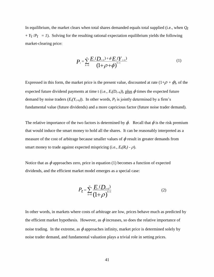
41

In equilibrium, the market clears when total shares demanded equals total supplied (i.e., when Qt

+ Yt /Pt = 1). Solving for the resulting rational expectation equilibrium yields the following

market-clearing price:

0

1

)1(

)()(

kk

kttktt

t

YEDEP

(1)

Expressed in this form, the market price is the present value, discounted at rate (1+ + ), of the

expected future dividend payments at time t (i.e., Et(Dt+k)), plus times the expected future

demand by noise traders (Et(Yt+k)). In other words, Pt is jointly determined by a firm’s

fundamental value (future dividends) and a more capricious factor (future noise trader demand).

The relative importance of the two factors is determined by . Recall that is the risk premium

that would induce the smart money to hold all the shares. It can be reasonably interpreted as a

measure of the cost of arbitrage because smaller values of result in greater demands from

smart money to trade against expected mispricing (i.e., Et(Rt) - ).

Notice that as approaches zero, price in equation (1) becomes a function of expected

dividends, and the efficient market model emerges as a special case:

0

1

)1(

)(

kk

ktt DE

(2)

In other words, in markets where costs of arbitrage are low, prices behave much as predicted by

the efficient market hypothesis. However, as increases, so does the relative importance of

noise trading. In the extreme, as approaches infinity, market price is determined solely by

noise trader demand, and fundamental valuation plays a trivial role in setting prices.

42

What factors affect ? Clearly characteristics of smart-money investors, such as their risk

aversion and wealth constraint, are important. More generally, arbitrage costs involve: 1)

trading costs: costs associated with establishing and closing the position; including brokerage

fees, price slippage, bid-ask spreads etc., 2) holding costs: costs associated with sustaining a

position; these costs are affected by factors such as the duration of the arbitrage position and the

incremental cost of short-selling a stock, and 3) information costs: costs associated with

information acquisition, analysis, and monitoring.27

Markets in which these three types of costs are low feature prices close to fundamentals. For

example, the markets for index futures and closed-end funds are characterized by relatively low

transaction and information costs. In these markets, valuation is relatively straightforward,

transaction costs are minimal, and the traded assets often have close substitutes. As might be

expected, the prices for these assets are closely tied to their fundamental values.28

In other markets, however, arbitrage costs ( ) can be potentially large, so noise traders

dominate. For example, the capital markets of many emerging economies feature relatively few

fundamental investors, little market depth and therefore high arbitrage costs. In domestic

markets, smaller firms, less closely followed and less actively traded stocks, and growth stocks

that are difficult to value will likely have higher arbitrage costs. The noise trader model predicts

that security prices in these markets will display more volatility, and will often seem to bear little

relation to their fundamental values.29

The main message from this model is that market prices are a product of the interplay between

noise traders and rational arbitrageurs, operating under cost constraints. Once we introduce

27 Shleifer and Vishny (1997) model the limits of arbitrage. We devote chapter 5 to this topic.

28 Even so, the evidence on closed-end fund discounts suggests that Yt exists and is mean-reverting (e.g., see Lee,

Shleifer, and Thaler (1991)).

29 Subsequent work by Baker and Wurlger (2006) provide strong support for this aspect of the Shiller model.

Specifically, Baker and Wurger show that, in the cross-section, a firm’s sensitivity to a measure of market-wide

sentiment (i.e., its “Sentiment Beta”) is indeed a function of arbitrage costs (measured by its idiosyncratic

volatility).

43

noise traders and costly arbitrage, price is no longer simply a function of future expected

dividends. Unless arbitrage costs are zero, Pt will not generally equal Vt. The magnitude of the

mispricing is a function of noise trader demand and arbitrage costs. More generally, when

arbitrage costs are non-zero, we can expect some mispricing to be an equilibrium phenomenon.

Another key insight is that the unpredictability of returns (a “no free lunch” version of the

efficient market hypothesis) does not guarantee price equals value (a “the price is right” version

of the efficient market hypothesis). Unfortunately, when the efficient market hypothesis is

invoked, it is often in the latter form. The fact that returns are largely unpredictable has been

widely interpreted as evidence in support of the fact that price equals the present value of

expected dividends. However, the model illustrates a conceptual problem with this general

approach to testing for market efficiency. In the model, returns may be unpredictable but stock

prices can still diverge dramatically from fundamental values.30

Finally, the model highlights the difference between fundamental analysis and security analysis.

Fundamental analysis is concerned with measuring firm value regardless of market conditions.

But in making security selections, smart-money investors need to consider the behavior of noise

traders, as well as fundamental valuation, in determining their own strategy. Smart money

investors need to consider “fashions” and “fads” in addition to “fundamentals.” Moreover, the

time-series behavior of Yt becomes important. If noise trader demand is random, then Pt is still

the best forecast of Vt. However, if Yt is mean reverting, then fundamental analysis is potentially

profitable. We expand on this point in the next chapter.

2.3 The Noise Trader Approach to Finance

It has now been three decades since Shiller published his model. In the ensuing years, behavioral

finance has continued to grow and expand as a subfield of economics. Interestingly, the key

30 For example, if arbitrage is costly (i.e., > 0) and noise trader demand (Yt) follows a random walk, the second

term in the numerator can be large, but stock returns are unpredictable. More generally, if Yt exhibits long-horizon

mean-reversion, rational traders with finite horizons would not be able to exploit the mispricing, even if it is

currently large.

44

features of this model have endured, and continue to be a useful organizing framework for much

of the subsequent work. Today, work on the “noise trader approach to finance” (Shleifer and

Summers (1990)) continues along three lines: (1) Firm fundamentals (or equity valuation), (2)

Investor sentiment (or non-fundamental price pressures), and (3) Limits to arbitrage. We will

take a closer look at each of the three components of the model in the next three chapters:

Chapter 3 (Equity Valuation), Chapter 4 (Investor Sentiment) and Chapter 5 (Limits to

Arbitrage). In the meantime, we present an extremely condensed synopsis of the three strands of

research.

2.3.1 Equity Valuation

A large literature examines the measurement of firm value based on fundamental analysis. Much

of the innovation has taken place in accounting in recent years, where the re-emergence of the

residual income model (RIM) has been central in pushing the research agenda.31 Although this

line of inquiry is not typically associated with behavioral finance, it fits well within the Shiller

framework. In the context of a noisy market price, an independent assessment of firm value

based on sustainable expected cash flows becomes central. Indeed, unless and until we have a

sensible measure of the value of firms based on expected payoffs to shareholders, it is difficult to

empirically distinguish between the two terms in the numerator of equation (1).

In Chapter 3 of this volume, we provide a review of some key insights gleaned from accounting-

based valuation theory. Our analysis demonstrates the inextricable conceptual link between a

stock’s “cheapness” (what the finance literature refers to as “the value effect”, typically

measured using various market multiples), and its “quality” (what the accounting fraternity

sometimes refers to as “fundamental pricing anomalies”, but which we believe are simply

accounting-based indicators of firm’s expected growth opportunities).

31 RIM had its origin in the early work of financial economists (e.g., Preinreich (1938), Edwards and Bell (1961),

Peasnell (1982), and Lehman (1993)). In the mid-1990s, a series of influential studies by James Ohlson (Ohlson

(1990, 1991, 1995), Feltham and Ohlson(1995)) helped accounting researchers to focus sharply on the importance of

the model as a means to understanding the relation between accounting data and firm value. Another key

contributor to this research has been Columbia professor Stephen Penman (see Penman (1997, 2010, and 2012)).

45

A key prediction of Shiller’s model is that, if arbitrage costs are non-trivial, sharper measures of

firm value will yield superior predictive power for future returns. As we show in Chapter 3, an

enormous body of evidence now suggests this is indeed the case.

2.3.2 Investor Sentiment

Broadly defined, investor sentiment refers to “optimism” (or “pessimism”) not justified by

existing fundamentals. Shiller envisioned traders who overreact/underreact to news, or are

vulnerable to fads and fashion trends, and much of his original article was devoted to a

discussion of noise trading as a social phenomenon. However, because the source of noise is

exogenous, what qualifies as investor sentiment in the model is in fact quite broad, and includes

for example the actions of those who trade for liquidity or consumption-based reasons. A

distinguishing feature of investor sentiment is that it is coordinated (or systemic) investor

demand of a non-fundamental nature, and thus the price pressure it generates will cause price to

move away from fundamental value.32

Subsequent empirical studies have used various techniques to measure market-wide sentiment.

Examples included the discount on closed-end funds (Lee, Shleifer, and Thaler (1991)), the

proportion of equity vs. debt issues by corporations (Baker and Wurgler (2000)), the consumer

confidence index (Lemmon and Portniaguina (2006)), the monthly fund flow between equity and

bond mutual funds within the same family (Ben-Raphael et al. (2012)), and a bottom-up measure

of aggregate corporate investment (Arif and Lee (2014)), and a composite sentiment index

(Baker and Wurgler (2006); Baker, Wurgler, and Yuan (2012)). See Baker and Wurgler (2007)

for a good summary.

Although investor sentiment is often viewed as a market-wide phenomenon, the concept of non-

fundamental price pressure is also highly relevant to the relative pricing of individual securities,

industries (e.g., e-commerce or biotech), geographical regions, or investment “styles” (e.g., value

versus growth, or low-volatility versus high-volatility). When certain stocks, industries, regions,

32 Unless noise trading is positively correlated across traders, or systemic, it will not affect price. Empirically,

trading records from individual brokerage accounts suggest noise trading is indeed systemic (e.g., Kumar and Lee

(2005)).

46

or styles of investing becomes “hot”, money flows in that direction, resulting in initial price

escalations, followed by subsequent return reversals. For example, an interesting line of research

examines the net inflows of money into various mutual funds, and documents how these flows

then impact future returns and the corporate actions of stocks held by the mutual funds (e.g.,

Coval and Stafford (2007), Frazzini and Lamont (2008), Lou (2012), Khan, Kogan, and Serafeim

(2012)).

More broadly, the literature on investor sentiment has examined the effect of signal saliency and

statistical reliability on the proclivity of investors to over- and under-weight individual signals.

Following the lead of psychologists (e.g., Kahneman and Tversky (1974), Griffin and Tversky

(1992)), researchers have observed a broad tendency for investors to over-weight signals that are

more salient or attention grabbing (e.g., Barber and Odean (2008), Hirshleifer, Lim, and Teoh

(2009), Da, Engelberg, and Gao (2011), and Engelberg, Sasseville, and Williams (2012)), and

under-weight signals that are statistically reliable but less salient, or required more processing to

be understood (e.g., Della Vigna and Pollet (2007), Gleason and Lee (2003), Giglio and Shue

(2012), Cohen and Lou (2012), Cohen, Diether, and Malloy (2013)).

In sum, the literature on investor sentiment is vast. We will touch on it again when discussing

value investing (Chapter 3) and will covered it in far more detail in Chapter 4. At this point, our

main message to accounting researchers is that stock prices can move for many reasons other

than a change in the present value of its expected future cash flows. These movements can be

large and persistent without being exploitable. Yet far from reducing the relevance of

fundamental analysis, this observation about markets actually elevates its importance.

2.3.3 Limits to arbitrage

The third element in the Shiller model is arbitrage costs (represented by ). In equilibrium

rational investors are compensated not only for bearing fundamental risk, but also for costs and

risks associated with noise trading. Subsequent analytical studies have provided more structure

by modelling various aspects of the costs faced by informational arbitrageurs, including: agency

problems raising from delegated asset management (Shleifer and Vishny (1997)), noise trader

47

risk (DeLong et al. (1990a, 1990b)), and a coordination problem faced by even sophisticated

investors (Stein (2009)).

More broadly, arbitrage costs encompass all costs and risks related to the exploitation of price

deviations from fundamental value. Once again, the idea of arbitrage costs is applicable at the

market level, the industry level, the style level, or the individual security level. At the individual

security level, Baker and Wurgler (2006) operationalize this concept using firm-level

idiosyncratic volatility as an empirical proxy. Many other studies have documented a

relationship between arbitrage constraints the magnitude of security mispricings (e.g., Pontiff

(1996), Mendenhall (2004), Mashruwala, Rajgopal and Shevlin (2006)). The role of short

selling has received particular attention (e.g., Blocher et al. (2013), Beneish et al. (2013),

Hirshleifer, Teoh, and Yu (2011)).

Increasingly, we find evidence that market frictions can have a dramatic effect on the pricing of

assets. For example, even in extremely liquid markets, such as monthly Treasury auctions,

dealers’ limited risk-bearing capacity and end-investors’ imperfect capital mobility can impact

prices and cause predictable patterns in future returns (Lou, Yan, and Zhang (2013)). The

influence of market frictions on prices is also highly time varying. For example, So and Wang

(2014) provide evidence that short-term return reversals in equity markets, a proxy for the

expected return market makers demand for providing liquidity, increase over six-fold

immediately prior to earnings announcements due to increased inventory risks associated with

holding net positions through the release of anticipated earnings news. At the same time, the

ability of market participants to assimilate news seems to be affected by their limited attention

span and processing power (Hirshleifer and Teoh (2003) and Hirshliefer et al. (2009)).

2.4 Implications for market-based research

We have argued that decoupling fundamental value from price is an important conceptual step

toward a richer research agenda. But, if price is not always equal to value, what role should

market prices play in our research design? How do we evaluate alternative estimates of value if

price is a noisy proxy for fundamental value? What specific areas of research appear particularly

promising at the moment? We turn now to these issues.

48

2.4.1 Suggestions for Future Research

What type of research will have the greatest impact in the future? Rather than generating a

laundry list, we will try to outline several features of salient research. Broadly speaking, we

believe the salient research in this area will be: 1) decision-driven, 2) interdisciplinary in nature,

and 3) prospective in focus.

Decision-driven. Many young researchers begin their quest for a research topic by reading

recent issues of academic journals. Given the lead time to publication at most of our top

academic outlets, these journals are not necessarily the best starting point for new research

projects. An alternative, and complementary, approach is to begin by identifying significant

economic decisions that utilize accounting data. In terms of generating ideas, practitioner

journals can be a good place to begin. The aim is to acquire an independent perspective on

topics that matter, in a broader economic context, before getting too close to the academic

literature itself.

Decision-driven research is not to be confused with product development or consulting. We are

not suggesting that we direct our research to practitioners. Rather, our call is for more research

that is based on careful observation of how decision makers behave, and how information signals

are used (or misused). Even basic research aimed at the theoretical foundations of our discipline

will benefit from more detailed knowledge of how important economic decisions are made.

Excellent examples of this type of research come from the literature on fundamental analysis. In

these studies, accounting-based variables are used to predict a variety of future outcomes. For

example, financial statement variables have been used to predict financial distress (Altman

(1968)) and future earning changes (Ou and Penman (1989)). They have proved useful in

assessing the persistence of earnings (Sloan (1996), Richardson et al. (2005)), improvements in

fundamentals (Piotroski (2000), Piotroski and So (2012)), and the probability of earnings

manipulation (Beneish (1999), Beneish et al. (2013)). Often, these variables also possess

predictive power for subsequent stock returns (see Richardson et al. (2010) for a good summary).

49

Interdisciplinary in nature. Few capital allocation decisions of significance involve solely the

use of accounting information. Therefore, it should not be surprising that the most important

accounting research in the capital market area will be interdisciplinary in nature. Solid training

in finance and economics is essential in these undertakings.

Some of the most interesting topics open to accountants today have traditionally been regarded

as the domain of corporate finance, asset pricing, or behavioral finance, even though accounting

information plays an important role in these decision contexts. In our view, accounting

researchers are likely to be better qualified to address many issues that arise in equity valuation,

share repurchases, LBOs, IPOs, loan syndications, mergers and acquisitions, and stock selection,

than their counterparts in finance. If we are willing to tackle these issues, accounting researchers

have the opportunity to generate some of the most significant research in financial economics

over the next few decades.

In addition, we believe it is now important for accounting researchers to be familiar with the

behavioral finance literature. Thaler (1999) predicts the demise of behavioral finance as a

separate branch of finance because he believes that, in the future, all of finance will be

behavioral. We are not at that stage yet, but the trend is unmistakably in this direction. In 2012,

the Journal of Financial Economics had a special issue on the topic of Investor Sentiment,

something unthinkable only a few decades ago.

We believe accountants also have an important role to play in understanding noise trader

demand. Unlike Keynes’ animal spirits, Shiller’s noise traders are not driven primarily by

idiosyncratic impulses or “a spontaneous urge to action” (Keynes (1936, page161)). Instead, the

mistakes in investor expectations are correlated across traders. Thus, Shiller does not model

individual irrationality so much as mass psychology or clientele effects. A common preference

or belief, which we might call investor sentiment, affects large groups of investors at the same

time.

What gives rise to these common sentiments (i.e., what affects Yt)? Shiller suggests sentiments

arise when investors trade on pseudo-signals, such as price and volume patterns, popular models,

50

or the forecasts of Wall Street gurus. More generally, Yt captures any price effect other than

those arising from the optimal use of dividend-related information. In this sense, noise trader

demand can be due either to sub-optimal use of available information, over- and under-reactions

to legitimate information signals, or responses to other exogenous liquidity shocks.33

The most salient feature of noise trader demand is that it drives price away from a stock’s

fundamental value. Therefore, as we refine our valuation tools, we simultaneously generate

better metrics for measuring noise trader demand. As information economists, accountants can

help identify signals (or pseudo-signals) that affect noise trader demand. We can also shed light

on the nature and extent of information processing costs (e.g., Demers and Vega (2011),

Engelberg (2008)), and how these costs impact corporate disclosure decisions (Blankespoor

(2013)). In fact, prior studies in accounting that investigate the under-utilization of information

in financial reports (e.g., Sloan (1996), and Richardson et al. (2005)) can be viewed as efforts to

identify noise trader preferences. Once we recognize that we can all be noise traders (that noise

traders are not a breed apart), the reconciliation with current accounting research is not difficult.

Prospective in focus. Much of accounting is historical in nature. A good deal of our research in

the capital market area has also tended to be retrospective and conducted within a framework

where stock return (or price) appears as the dependent variable and contemporaneous accounting

data appear as independent variables. According to this widely utilized paradigm, accounting

data that better explain contemporaneous returns (or prices) are presumed to be superior in some

normative sense.

However, as pointed out by Bernard (1995; page 743), this paradigm is limiting because it

"precludes from the outset the possibility that researchers could ever discover something that was

not already known by the market." As our view on market efficiency changes, we believe a

greater emphasis will be placed on research that helps predict the outcome of future economic

events. This research will have as a primary focus the goal of enhancing capital allocation

33 In the noisy rational expectation literature, the noise introduced by exogenous liquidity shocks is crucial in

inducing trading and in limiting the extent to which price reveals full information. For an example of this type of

model, see Grossman and Stiglitz (1980) or Diamond and Verrecchia (1981).

51

decisions whose outcomes are not yet known. It will include, but not be limited to, studies that

help to forecast future stock returns.

Each year the American Accounting Association (AAA) awards a Notable Contributions to

Accounting Literature Award. The recipient(s) of this award have written, in the view of the

selection committee, the most influential study in accounting over the past five years. The

subject matters covered by the past winners are diverse, and include: earnings quality, cost-of-

capital, equity valuation, financial statement analysis, managerial accounting, auditor judgment,

international accounting standards, and corporate governance.34 But even a cursory review of

these winners will make plain the importance of focusing on decision-relevant and

interdisciplinary research of a prospective nature.

2.5 Research Design Issues

If the stock price itself is a noisy measure for a firm’s true fundamental value, how should we

proceed in designing our research studies? How do we model the relation between value and

price? This is a matter of obvious import as we leave the comfortable confines of the efficient

market paradigm. Future researchers will need to grapple with this matter more thoroughly, but

the following two empirical studies might serve to illustrate the possibilities. Both are what we

regard as “hybrid” studies that do not discard the information in market price completely, but

rely on weaker assumptions about the relation between price and fundamental value.

First, Lee, Myers and Swaminathan (1999) (LMS) models price and value as a co-integrated

system -- in other words, the observed price and the accountant's estimate of value both measure

the true (but unobservable) fundamental value with noise. In this context, they examine the

question of how value estimates based on accounting numbers should be evaluated. They show

that in this framework, under fairly general conditions, superior value estimates will not only be

more correlated with contemporaneous returns, but will also yield better predictions of future

returns.

34 See http://aaahq.org/awards/awrd3win.htm

52

In the LMS model, prices and value are assumed to be long-term convergent due to arbitrage

forces. However, in the spirit of the noise trader model discussed in the prior section, at any

given point in time market price can diverge from the true (but unobserved) fundamental value.

In this context, the role of fundamental analysis is to generate an independent value estimate that

helps to discipline the observed price. Their analysis suggests two benchmarks for evaluating

the degree to which an accountant’s empirical value estimate has been successful in capturing

true fundamental value. Specifically, LMS argues that superior measures of true intrinsic value

will be better able to: (a) track price variation over time, and (b) predict of future returns. Using

these two performance metrics, they provide evidence on the usefulness of various inputs into

the RIM model – such as analyst forecasts, time-varying discount rates, etc.

Second, Gebhardt, Lee, and Swaminathan (2000) (GLS) use a discounted residual income model

to generate a market implied cost-of-capital. They then examine firm characteristics that are

systematically related to this cost-of-capital estimate. They show that a firm’s implied cost-of-

capital is a function of its industry membership, B/M ratio, forecasted long-term growth rate, and

the dispersion in analyst earnings forecasts. Together, these variables explain around 60% of the

cross-sectional variation in future (two-year-ahead) implied costs-of-capital. The stability of

these long-term relations suggests they can be exploited to estimate future costs-of-capital.35

Contrary to the concerns raised in Kothari (2001), the research design in GLS is not based on an

assumption of market efficiency in the traditional sense (i.e., Pt = Vt, t). For purposes of stock

selection, it would be tautological to estimate the implied cost-of-capital based on current stock

prices. In fact, the cost-of-capital estimate recommended in GLS does not rely on a firm’s

current market price. Rather, GLS relies on long-term relations between the market implied

cost-of-capital and various firm characteristics to estimate an “expected” or “warranted” cost-of-

capital for each firm. This warranted cost-of-capital is then compared to the “actual implied”

35 An important caveat is that a substantial part of this explanatory power derives from the fact that the implied cost-

of-capital is correlated with firm characteristics, such as the B/M ratio.

53

cost-of-capital derived from the current price. Trading strategies are based on the “spread”

between the warranted and actual measures.36

Both studies implicitly assume a weaker form of market efficiency than is commonly found in

the literature. Specifically, these studies assume that price and value are locked together in the

long run by arbitrage forces. Price contains valuable information about future payoffs that

should not be ignored. However, at any given point in time, price also departs from fundamental

value due to exogenous forces (or, in the parlance of behavioral finance, noise trader demand).

The authors in these studies exploit the long-term relation between accounting fundamentals and

market prices to gauge short-term price deviations. We refer to this as a “hybrid” approach,

because it utilizes both accounting fundamentals and past prices to predict future prices.

Returning to the ocean analogy, these studies use the average level of the ocean (i.e., the long-

term market valuation of certain fundamentals) to measure the current height of the tides (the

current market valuation of the same fundamentals).

2.6 Summary

The existence of Noise Traders is a centerpiece of the noise trader model (NTM). In simple

terms, investor sentiment (or noise trader demand) may be defined as any investor demand or

price pressure not aligned with news about fundamentals. In the NTM, investor sentiment can

cause prices to move away from fundamental value. Investor sentiment could be driven either by

differential liquidity needs, preferences, or information sets; or alternatively by behaviorally

induced biases in the assessment of currently available information.

36 This approach is analogous to fixed income arbitrageurs who routinely compare the warranted yield on bonds to

the actual yield at a given point in time to uncover profit opportunities. Bhojraj and Lee (2002) demonstrate how

warranted multiples can help identify peer firms. In practice, many quantitative asset managers already implicitly

make such an adjustment when they neutralize their value signals to industry, size, and other firm characteristics that

consistently explain firms’ implied cost of capital.

54

Although the idea that noise traders can affect prices is often identified with the behavioral

finance literature, it is not unique to this literature. Noise traders were an integral part of the

noisy rational expectation models and the Kyle (1985) models in market microstructure. In these

models, noise traders trade for exogenous liquidity reasons. What is unique about the behavioral

models is that these traders are assumed to trade not only for liquidity reasons, but also because

they also tend to misperceive the present value of firms’ future fundamentals.

In the NTM, the demand of noise traders affects prices in at least three important ways. First, the

synchronized activities of noise traders is the reason prices deviate away from fundamentals, thus

their collective actions are the primary source of the market mispricing in equilibrium. At the

same time, as Black (1986) observed, it is noise trader demand that provides the opportunity for

smart money to earn a higher return by investing in information acquisition and analysis.

Therefore, while noise traders cause mispricing, they are also the ultimate source of funding for

the arbitrageurs (smart money).

Second, noise trading is a key source of market risk, which is priced in equilibrium. The fact

that the actions of these noise traders are difficult to predict introduces an additional element of

risk to all market participants. This is seen as the risk premium associated with arbitrage costs

(the ϕ parameter), which appears in the denominator of the market clearing price. Finally, the

severity of the effect of noise trading is also related to the cost of arbitrage. Specifically, the

magnitude of the mispricing is a function of how costly it is for smart money to eliminate the

activities of the noise traders.37

This noise trader demand might come from exogenous liquidity shocks that are non-fundamental

in origin. In the ensuing years, an extensive literature on investor sentiment and noise trading has

emerged, with implications for empirical asset pricing, corporate finance, financial accounting,

and macroeconomics. More complex and sophisticated models have been developed that

attempt to provide more structure on the dynamics of noise trading and under various forms of

37 For simplicity, the model assumes noise trader demand is exogenous. In reality, the nature and extent of expected

noise trader demand (the Et(Yt+i)) term) is unlikely to be independent from the size of the risk premium smart money

demands for holding the risky asset (the ϕ term).

55

constrained arbitrage.38 However, simple as it may seem, the basic framework outline in

Shiller’s 1984 study has survived largely intact in literature today.

38 For example, DeLong et al. (1990a, 1990b), Barberis, Shleifer, and Vishny (1998), Hong and Stein (1999), and

Daniel, Hirshleifer, and Subrahmanyam (2001).

56

References

Altman, E. I. 1968. Financial ratios, discriminant analysis, and the prediction of corporate

bankruptcy. Journal of Finance 23: 589-609.

Arif, S., and C. M. C. Lee, 2014, Aggregate investment and investor sentiment, Review of

Financial Studies, forthcoming.

Baker, M., and J. Wurgler. 2000. The equity share in new issues and aggregate stock returns,

Journal of Finance 55:2219-57.

, 2006, Investor sentiment and the cross-section of stock returns. Journal of

Finance 61, 1645-1680.

_____________, 2007, Investor Sentiment in the stock market, Journal of Economic

Perspectives 21, 129-151.

Baker, M., J. Wurgler, and Y. Yuan. 2012. Global, local, and contagious investor sentiment.

Journal of Financial Economics 104:272-87.

Barber, B., and T. Odean, 2008, All that glitters: The effect of attention and news on the buying

behavior of individual and institutional investors, Review of Financial Studies 21(2), 785–

818.

Barberis, N., 2013, Thirty years of prospect theory in economics: a review and assessment,

Journal of Economic Perspectives 27:1, 173-196.

Barberis, N., and M. Huang, 2008, Stocks as lotteries: The implications of probability weighting

for security prices, American Economic Review 98(5), 2066-2100.

Barberis, N., M. Huang, and T. Santos, 2001, Prospect theory and asset

prices, Quarterly Journal of Economics 116, 1-53.

57

Barberis, N., A. Shleifer, and R. Vishny, 1998, A model of investor sentiment, Journal of

Financial Economics 49, 307-343.

Barberis, N., and R. Thaler, 2002, A survey of behavioral finance, Handbook of the Economics

of Finance, Chapter 18, edited by G. M. Constantinides, M. Harris, and R. Stulz. Elsevier

Science B. V.

Beneish, M.D. 1999. The detection of earnings manipulation. Financial Analysts Journal

(September/October): 24-36.

Ben-Rephael, A., S. Kandel, and A. Wohl, 2012, Measuring investor sentiment with mutual fund

flows, Journal of Financial Economics 104, 363-382.

Bernard, V. L., 1995, The Feltham-Ohlson framework: implications for empiricists,

Contemporary Accounting Research 11, 733-747.

Bernard, V. L., and J. K. Thomas, 1990, Evidence that stock prices do not fully reflect the

implications of current earnings for future earnings, Journal of Accounting and Economics

13, 305-341.

Bhojraj, S. and C. M. C. Lee, 2002, Who is my peer? A valuation-based approach to the

selection of comparable firms, Journal of Accounting Research 40(2), 407-439.

Black, Fischer, 1986, Presidential address: Noise, Journal of Finance 41, 529-543.

Blankespoor, E., 2013, The impact of information processing costs on firm disclosure choice:

evidence from the XBRL mandate, Stanford University working paper, August.

Blocher, J., A. V. Reed, and E. D. Van Wesep, 2013, Connecting two markets: An equilibrium

framework for shorts, longs, and stock loans, Journal of Financial Economics 108, 302-

322.

58

Cohen, L., K. Diether, and C. Malloy, 2013, Misvaluing innovation, Review of Financial Studies,

forthcoming.

Cohen, L., and D. Lou, 2012, Complicated firms, Journal of Financial Economics 91, xxx-yyy.

Coval J., and E. Stafford, 2007, Asset fire sales (and purchases) in equity markets. Journal of

Financial Economics 86, 479-512.

Cutler, D., J. Poterba, and L. Summers, 1989, What moves stock prices? Journal of Portfolio

Management, Spring, 4-12.

Da, Z., J. Engelberg, and P. Gao, 2011, In search of attention, Journal of Finance 66, 1461-1499.

Daniel, K., Hirshleifer, D., and A. Subrahmanyam, 1998, Investor Psychology and

security market under- and overreactions, Journal of Finance 53, 1839-1886.

, 2001, Overconfidence, arbitrage, and equilibrium asset pricing, Journal of

Finance 56, 921-965.

Della Vigna, S., and J. M. Pollet, 2007, Demographics and Industry Returns. American

Economic Review 97, 1667-1702.

Demers, E., and C. Vega, 2011, Linguistic tone in earnings press releases: news or noise?

INSEAD and the Board of Governors of the Federal Reserve System, Working Paper, May.

De Long, J. B., A. Shleifer, L. H. Summers, and R. J. Waldmann, 1990a, Noise trader risk in

financial markets, Journal of Political Economy 98, 703-738.

________________, 1990b, Positive feedback investment strategies and destabilizing rational

speculation, Journal of Finance 45, 375-395.

Diamond, D. W., and R. E. Verrecchia, 1981, Information Aggregation in a Noisy Rational

Expectations Economy, Journal of Financial Economics 9, 221-236.

59

Drake, M. S., L. Rees, and E. P. Swanson, 2010, Should investors follow the prophets or the

bears? Evidence on the use of public information by analysts and short sellers, The

Accounting Review 86:1, 101-130.

Edwards, E. O., and P. W. Bell, 1961, The Theory and Measurement of Business Income,

University of California Press, Berkeley, CA.

Engelberg, J., 2008, Costly information processing: Evidence from earnings announcements,

Northwestern University, Working Paper, January.

Engelberg, J., C. Sasseville, and J. Williams, 2012, Market madness? The case of Mad Money,

Management Science 58, 351-364.

Feltham, G. A., and J. A. Ohlson, 1995, Valuation and clean surplus accounting for operating

and financial activities, Contemporary Accounting Research 11, 689-731.

Frazzini, A., and O. A. Lamont. 2008. Dumb money: Mutual fund flows and the cross-section

of stock returns. Journal of Financial Economics 88, 299-322.

Gebhardt, W., Lee, C. M. C., and B. Swaminathan, 2001, Toward an implied cost of capital,

Journal of Accounting Research 39, 135-176.

Giglio, S. and K. Shue, 2012, The news to no news: does the market underreact to nothing?

University of Chicago Booth School, Working Paper, August 31.

Gleason, C., and C. M. C. Lee, 2003, Analyst forecast revisions and market price discovery, The

Accounting Review 78, 193-225.

Griffin, D., and A. Tversky, 1992, The weighing of evidence and the determinants of confidence,

Cognitive Psychology 24, 411-35.

60

Grossman, S., and J. E. Stiglitz, 1980, On the impossibility of informationally efficient markets,

American Economic Review 70, 393-408.

Hirshleifer, D., 2001, Investor psychology and asset pricing, Journal of Finance 56, 1533-1597.

Hirshleifer, D., S. S. Lim, and S. H. Teoh, 2009, Driven to distraction: Extraneous events and

underreaction to earnings news, Journal of Finance 64, 2289-2325.

Hirshleifer, D., and T. Shumway, 2003, Good day sunshine: Stock returns and the weather,

Journal of Finance 58, 1009–1032.

Hirshleifer, D., and S. H. Teoh, 2003, Limited attention, information disclosure, and financial

reporting, Journal of Accounting and Economics 36, 337–386.

Hirshleifer, D., S. H. Teoh, and J. J. Yu, 2011, Short arbitrage, return asymmetry, and the accrual

anomaly, Review of Financial Studies 24(7), 2429-2461.

Hong, H., and J. C. Stein, 1999, A unified theory of underreaction, momentum trading and

overreaction in asset markets, Journal of Finance 54, 2143-2184.

Kahneman, D., and A. Tversky, 1974, Judgment under uncertainty: heuristics and biases, Science

185, 1124-31.

Keynes, J. M., 1936, The general theory of employment, interest, and money, Chapter 12, First

Harvest/HBJ edition 1964. Harcourt Brace Jovanovich: New York.

Khan, M., L. Kogan, and G. Serafeim, 2012, Mutual Fund Trading Pressure: Firm-Level Stock

Price Impact and Timing of SEOs, Journal of Finance 67 (4), 1371-1395.

Kothari, S. P., 2001, Capital market research in accounting, Journal of Accounting and

Economics 31(1), 105-231.

61

Kumar, A., and C. M. C. Lee, 2006. Retail investor sentiment and return comovements,

Journal of Finance 61, 2451-2486.

Kyle, A. S., 1985, Continuous auctions and insider trading. Econometrica: Journal of the

Econometric Society, 1315-1335.

Lee, C., Myers, J., and B. Swaminathan, 1999, What is the intrinsic value of the Dow? Journal of

Finance 54, 1693-1741.

Lee, C. M. C., A. Shleifer and R. Thaler, 1991, Investor sentiment and the closed-end fund

puzzle, Journal of Finance 46, 75-109.

Lehman, B., 1993, Earnings, dividend policy, and present value relations: Building blocks of

dividend policy invariant cash flows, Review of Quantitative Finance and Accounting 3,

263-282.

Lemmon, M. and E. Portniaguina. 2006. Consumer confidence and asset prices: Some

empirical evidence. Review of Financial Studies 19:1499-1529.

Ljungqvist, A., and W. Qian, 2014, How constraining are limits to arbitrage? NYU Stern School

and NUS Business School working paper, May 6.

Lou, D., 2012, A flow-based explanation for return predictability, Review of Financial Studies

25(1), 3457-3489.

Lou, D., H. Yan, and J. Zhang, 2013, Anticipated and repeated shocks in liquid markets, Review

of Financial Studies 26(8), 1890-1912.

Mashruwala, C., S. Rajgopal, and T. Shevlin, 2006, Why is the accrual anomaly not arbitraged

away? The role of idiosyncratic risk and transaction costs, Journal of Accounting and

Economics 42, 3-33.

62

Mendenhall, R., 2004, Arbitrage risk and post-earnings-announcement drift, Journal of Business

77(4), 875-894.

Ohlson, J. A., 1990, A synthesis of security valuation theory and the role of dividends, cash

flows, and earnings, Contemporary Accounting Research 6, 648-676.

, 1991, The theory of value and earnings, and an introduction to the Ball-

Brown analysis, Contemporary Accounting Research 7, 1-19.

, 1995, Earnings, book values, and dividends in security valuation,

Contemporary Accounting Research 11, 661-687.

Ou, J. A. and S. H. Penman. 1989. Financial statement analysis and the prediction of stock

returns. Journal of Accounting & Economics 11 (4): 29-46.

Peasnell, K., 1982, Some formal connections between economic values and yields and

accounting numbers, Journal of Business Finance and Accounting 9, 361-381.

Penman, S. H., 1997, A synthesis of equity valuation techniques and the terminal value

calculation for the dividend discount model, Review of Accounting Studies 2, 303-323.

, 2010, Accounting for value, Columbia University Press.

, 2012, Financial statement analysis and security valuation, Fifth Edition,

McGraw-Hill/Irwin.

Piotroski, J., 2000, Value investing: The use of historical financial statement information to

separate winners from losers, Journal of Accounting Research 38, 1-41.

63

Piotroski, J. D., and E. C. So, 2012, Identifying expectation errors in value/glamour strategies: A

fundamental analysis approach, Review of Financial Studies, forthcoming.

Pontiff, J., 1996, Costly arbitrage: evidence from closed-end funds, Quarterly Journal of

Economics 111, 1135-1152.

Preinreich, G., 1938, Annual survey of economic theory: The theory of depreciation,

Econometrica 6, 219-241.

Richardson, S. A., R. G. Sloan, M. T. Soliman, and I. Tuna. 2005. Accrual reliability, earnings

persistence and stock prices. Journal of Accounting & Economics 39 (3): 437-485.

Richardson, S., R. Sloan, and H. You, 2012, What makes stock prices move? Fundamentals vs

investor recognition. Financial Analysts Journal 68:2, 30-50.

Rubinstein, M., May/June 2001, Rational markets: Yes or No? The affirmative

case, Financial Analysts Journal 5, 15-29.

Shiller, R. J., 1984, Stock prices and social dynamics, The Brookings Papers on Economic

Activity 2, 457-510.

Shleifer, A., 2000, Inefficient markets: an introduction to behavioral finance, Chapter 1, Oxford

University Press.

Shleifer, A., and L. Summers, 1990, The noise trader approach to finance, Journal of Economic

Perspectives 34, 19-33.

Shleifer, A., and R. W. Vishny, 1997, The limits of arbitrage, Journal of Finance 52, 35-55.

Sloan, R., 1996, Do stock prices fully reflect information in accruals and cash flows about future

earnings? The Accounting Review 71, 289-316.

64

So, E., and S. Wang, 2014, News-driven return reversals: Liquidity provision ahead of earnings

announcements, Journal of Financial Economics, forthcoming.

Stein, J. C., 2009, Presidential address: Sophisticated investors and market efficiency, Journal of

Finance 64, 1517-1548.

Thaler, R., 1999, The end of behavioral finance, Financial Analysts Journal 55, 12-17.

Tversky, A. and D. Kahneman, 1981, The framing of decisions and the psychology of choice,

Science 211, 453-458.

65

Chapter 3

Equity Valuation

This chapter offers an introduction to equity valuation with the goal of building a bridge between

the theory and practice of value investing. We review some key insights gleaned from

accounting-based valuation theory to demonstrate the inextricable conceptual link between a

stock’s “cheapness” and its “quality”. We then use these insights as an organizing framework to

discuss the essence of intelligent value investing.

We also discuss the implications of accounting-based valuation theory for market efficiency.

Using examples from the asset management industry, we illustrate the key role played by equity

valuation in informing investment decisions. At the same time, we show how seemingly

disparate strands of empirical evidence in academic studies about the predictive power of

historical accounting variables for stock returns, in fact, dovetail nicely with the investment

philosophy of such legendary investors as Ben Graham, Warren Buffett, and Joel Greenblatt.

Finally, the chapter ends with a discussion of whether value investing will continue to be

profitable in the future. In doing so, we survey potential explanations for the long-standing

success of value investing discussed in the academic literature.

3.1 Overview

Value investing refers to the buying or selling of stocks on the basis of a perceived gap between

a firm’s market price and its intrinsic value. What is the intrinsic value of a firm? Here is a

simple and relatively non-controversial definition.

“The intrinsic (equity) value of a firm is the present value of expected

future payoffs to shareholders.”

Unlike rare art, stocks are commonly presumed to have an intrinsic value. The intrinsic value of

a Van Gogh painting is ill defined; basically, its value is what people are willing to pay for it.

But when investors think about equity valuation, we have in mind a monetary sum that

66

corresponds to the present value of expected future payoffs to shareholders. Each share, after all,

is simply a fractional ownership claim on an on-going business enterprise. In contrast to other

assets that carry non-monetary benefits (such as the consumptive value of the house we live in,

or the pleasure derived from owning a painting), stocks derive their value, by and large, from

their claim to a firm’s future cash flows. Valuing these future cash flows is an integral part of

value investing because it provides investors with an independent measure of firm value that

could be used to challenge and perhaps discipline the current market price.

Value investors buy stocks that appear to be cheap relative to their intrinsic value, and sell (even

sell short) stocks that seem expensive. One of the most remarkable regularities in the empirical

asset pricing literature has been the fact that value investing is consistently associated with

positive abnormal returns. Both empirical academic studies and the evidence from a host of

professional asset managers seem to confirm this. A substantial literature in finance and

accounting shows that firms trading at lower pricing multiples, with stronger balance sheets,

more sustainable cash flows, higher profitability, lower volatility, lower Beta, and lower distress

risk, actually earn higher, not lower, future stock returns. This pattern in cross-sectional returns,

which we refer to collectively as the “value effect”, was first recognized by famed Columbia

University professor, Benjamin Graham, and documented as early as 1934. Various elements of

this effect have been confirmed (and rediscovered) by a host of academic studies in the ensuing

80 years.

A common misconception among many academics and financial practitioners is that “value” is

equivalent to “cheapness.” Thus in many academic studies, “value stocks” are defined simply as

those trading at lower market multiples (i.e., lower M/B, P/E, CF/P, etc.).39 This chapter

illustrates that sensible value investing is not merely finding “cheap” stocks; it requires finding

“quality” stocks (firms with strong fundamentals) trading at reasonable prices. We will provide

some examples of how accounting numbers can be used, and are indeed being used, by

successful professional investors to identify quality stocks. In fact, we believe many recent

39 For example, Fama and French (1992), Lakonishok, Shleifer, Vishny (1994).

67

results from academic research are extremely useful to value investors in their search for quality

companies trading at reasonable prices.

In the remainder of this chapter, we revisit the theoretical underpinnings of the value effect, and

summarize what is now an extensive body of evidence in support of its existence. We will get to

the theory part shortly, but let us once again begin with an illustration, this time taken from the

writings of Benjamin Graham.

3.2 Benjamin Graham as a Quant

In one of the earliest editions of Security Analysis, which he co-authored with David Dodd in

1934, Graham proposed a simple stock screen. While the numbers in the screen have varied

slightly across editions, the original form of this screen is preserved. Here is the original

screen.40 Any stock that possesses all 10 of the following characteristics, according to Graham,

would be a worthwhile investment:

1. Earnings to price ratio that is double the AAA bond yield.

2. PE of the stock has less than 40% of the average PE for all stocks over the last 5

years.

3. Dividend Yield > Two-thirds of the AAA Corporate Bond Yield.

4. Price < Two-thirds of Tangible Book Value.

5. Price < Two-thirds of Net Current Asset Value (NCAV), where net current asset

value is defined as liquid current assets including cash minus current liabilities.

40 We are indebted to Professor Aswath Damodaran for bringing our attention to this screen. See Damodaran

(2012) for an excellent historical perspective on value investing. See Cottle, Murray, Block(1988) for a more recent

version of the Graham and Dodd classic.

68

6. Debt-Equity Ratio (Book Value) has to be less than one.

7. Current Assets > Twice Current Liabilities.

8. Debt < Twice Net Current Assets.

9. Historical Growth in EPS (over last 10 years) > 7%.

10. No more than two years of declining earnings over the previous ten years.

When presenting this screen, we ask students to group these 10 factors into two general

categories (that is, find five factors that have more in common with each other than with the

other five factors). If you stare at this screen for a few moments, you will notice that there are in

fact two natural groupings. The first five factors appear to be more closely linked to each other

than they are to the next five factors that follow.

You might also recognize that the first five factors are all measures of “cheapness”. The first

two factors compare a company’s stock price to their reported earnings, and encourage us to buy

stocks whose P/E ratio is below a certain threshold. The next three compare a stock’s price to its

dividends, book value, and net current asset value (NCAV), respectively. Taken together, these

first five factors are all instructing us to buy companies whose prices are “cheap” relative to

reference measures extracted from historical financial statements.

The next five factors differ from the first five in that they do not involve the stock price. As a

group, we might refer to these five factors as measures of a firm’s “quality”. Notice that these

factors are pure accounting constructs: financial ratios or growth rates; accounting numbers over

accounting numbers. Factors 6 through 8 measure debt (or leverage), as well as short-term

liquidity (or solvency). Factors 9 and 10 are measures of a company’s historical earnings growth

rate and the consistency of that growth. In short, Graham wants to buy firms with low leverage,

high solvency, and a high and consistent rate of growth, sustained over a period of time. Quality

69

firms, according to Ben Graham, are those with high and steady growth, low leverage, and ample

liquidity.

Does this strategy work? A few years ago, a Stanford University MBA student, Becca Levin,

designed a slightly updated version of this screen. Becca used the same basic formulation as

Graham, but updated a couple of the constructs (substituting free-cash-flow yield, for example,

in place of dividend yield; and requiring just 5-years of past earnings growth rather than 10-

years). We recently conducted a test of this strategy using a dataset of U.S. companies over the

most recent 14 years (1/2/1999 to 11/9/2013).

The Levin-Graham strategy is quite simple to implement. Specifically, we assign a +1 score if a

firm meets each condition; top firms can receive a maximum score of 10, bottom firms can score

as low as 0. At the beginning of each quarter, all firms are sorted into 10 portfolios according to

their Levin-Graham score. We then compute the equal-weighted return for each of these 10

portfolios over the next three months. The test is performed using “as reported” Compustat data,

with no survivorship or restatement issues. All variables are computed using publicly available

data as of the date of portfolio formation (no “peek ahead” bias). To avoid illiquid stocks, we

include only firms with a price of $3 or more. The results are reported in Figure 1.

[Insert Figure 1]

This figure reports the equal-weighted return to each of these 10 portfolios over the next three

months (annualized, assuming quarterly rebalancing).41 The right-most column represents EW-

returns to a portfolio of firms with the highest score, and so on. The eleventh (left-most) column

is the return to the S&P400 Midcap (value-weighted) index over the same time period, included

for comparison.

41 Note that value investors can employ two related sets of strategies. The first set is comprised of fundamentally

oriented value strategies such as Levin-Graham screen presented above that tend to be more focused on comparing

price relative to value for a given firm. The second set is comprised of systematically oriented value strategies that

compare valuation metrics across related firms in the cross-section. See Land and Lundholm (1996) for a discussion

of the potential difference in the impacts these strategies on price formation.

70

Remarkably, this 80-year-old screen continues to predict stock returns in the 21st century! In

general, cheaper and higher quality stocks earn higher returns over the next 3-months. On an

annualized basis, firms in the top two-deciles of the screen averaged around 14% per year, while

firms in the bottom two-deciles averaged around 5%. The difference between these stocks is 9%

per year (or equivalently, around 2.25% per quarterly rebalancing period). For comparison, the

value-weighted S&P400 Midcap index returned only 8.5% over this time period. The decile

results are not monotonic, but by and large, we see that cheaper and higher-quality stocks do earn

higher returns even in the most recent 14 year period, in what is arguably the most efficient stock

market in the world.

3.3 A Bit of Theory Might Help

What might account for this performance? Was this an unusual time period in U.S. history? To

proceed further, we need to introduce a bit of valuation theory.

The Residual Income Model (RIM)

In the early to mid-1990s, Professor James Ohlson wrote a series of influential studies on equity

valuation featuring what became known as the “residual income model” (RIM).42

The RIM had

its origin in the early work of financial economists.43

Although the original model predates his

work by several decades, Ohlson helped many academics to refocus on the importance of the

RIM as a means to understanding the relation between accounting data and firm value.44

The most common form of the RIM in the academic literature expresses a firm’s value in terms

of its current book value and future expected abnormal accounting rates-of-returns:

42 Ohlson (1990, 1991, 1995), Feltham and Ohlson (1995).

43 See, for example, Preinreich (1938), Edwards and Bell (1961), Peasnell (1982), and Lehman (1993).

44 Bernard (1995), Lundholm (1995), and Lee (1999) offer less technical discussions on the implications of Ohlson's

work. Many excellent books, including Healy and Palepu(2012), Penman (2010, 2012), and Whalen, Baginski, and

Bradshaw (2010), discuss implementation details. Ohlson often underscores the fact that a RIM lacks content

without additional assumptions (for example, the “Linear Information Dynamics” assumptions in Ohlson (1995)).

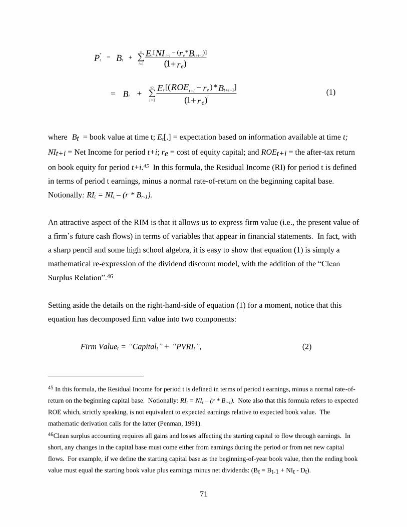
71

1

1*

)1(

)]*([

ii

iteitt

tt

r

BrNIEBP

e

1

1

)1(

( ]*)[

ii

iteitt

t

r

BrROEEB

e

(1)

where Bt = book value at time t; Et[.] = expectation based on information available at time t;

NIt+i = Net Income for period t+i; re = cost of equity capital; and ROEt+i = the after-tax return

on book equity for period t+i.45 In this formula, the Residual Income (RI) for period t is defined

in terms of period t earnings, minus a normal rate-of-return on the beginning capital base.

Notionally: RIt = NIt – (r * Br-1).

An attractive aspect of the RIM is that it allows us to express firm value (i.e., the present value of

a firm’s future cash flows) in terms of variables that appear in financial statements. In fact, with

a sharp pencil and some high school algebra, it is easy to show that equation (1) is simply a

mathematical re-expression of the dividend discount model, with the addition of the “Clean

Surplus Relation”.46

Setting aside the details on the right-hand-side of equation (1) for a moment, notice that this

equation has decomposed firm value into two components:

Firm Valuet = “Capitalt” + “PVRIt”, (2)

45 In this formula, the Residual Income for period t is defined in terms of period t earnings, minus a normal rate-of-

return on the beginning capital base. Notionally: RIt = NIt – (r * Br-1). Note also that this formula refers to expected

ROE which, strictly speaking, is not equivalent to expected earnings relative to expected book value. The

mathematic derivation calls for the latter (Penman, 1991).

46Clean surplus accounting requires all gains and losses affecting the starting capital to flow through earnings. In

short, any changes in the capital base must come either from earnings during the period or from net new capital

flows. For example, if we define the starting capital base as the beginning-of-year book value, then the ending book

value must equal the starting book value plus earnings minus net dividends: (Bt = Bt-1 + NIt - Dt).

72

where the book value at period t is “Capitalt”, or the initial Invested Capital base, and the rest of

the right-hand-side is the “Present Value of Future Residual Income”, hereafter referred to as

“PVRIt”.

Equation (2) highlights the fact that Firm Value (what the firm is worth today), is always a

function of two components: Invested capital (the asset base we start with today), and “Present

Value of Future Residual Income” (where this asset base is going; in other words, our projection

of the future value-enhancing growth in the capital base).

As it turns out, what we use as our starting capital base (Capitalt) really does not matter (see

Penman (1996, 1997)). In equation (1), the current book value was used as the starting capital,

but we could have chosen virtually any number as a starting capital. So long as our forecasts

obey two simple rules of internal consistency, the resulting Firm Value estimate will be

equivalent to the present value of a firm’s future dividends.47

Subsequent studies featured several alternative measures of the invested capital base other than

book value. For example, a firm’s capitalized one-year-ahead earnings forecast, or its current

year sales revenue.48 The general RIM formula tells us that, for each invested capital choice, we

can derive an equivalent expression for the present value of the corresponding residual income

term. In other words, for each Capitalt selected, we can compute a matching PVRIt such that the

sum will always be mathematically equivalent to the present value of future payout to

shareholders.49

47 The two consistency requirements are: First, the three elements of RI need to be consistently defined: Having

specified the capital base (Capitalt), Earningst must be the income to that capital base in year t, and r must be the

cost-of-capital associated with this source of capital. Second, the evolution of the capital base in this model must

follow the Clean Surplus Relation (CSR).

48 For example, Ohlson and Juettner-Nauroth (2005) and Easton (2004) use capitalized one-year-ahead earnings

(EARNt+1) as the starting capital base in developing the Abnormal Earnings Growth Model (AEGM). Bhojraj and

Lee (2002) use the RIM formula to estimate a matching PVRI for each firm’s enterprise-value-to-sales (EV/S) ratio.

49 Although the arithmetic carries through, clearly not all measures of capital are equally sensible from an economic

perspective. A full analysis of which “capital-in-place” measures might be more sensible is beyond the scope of the

current discussion. However, it might be worth noting in passing that granting greater latitude to management in

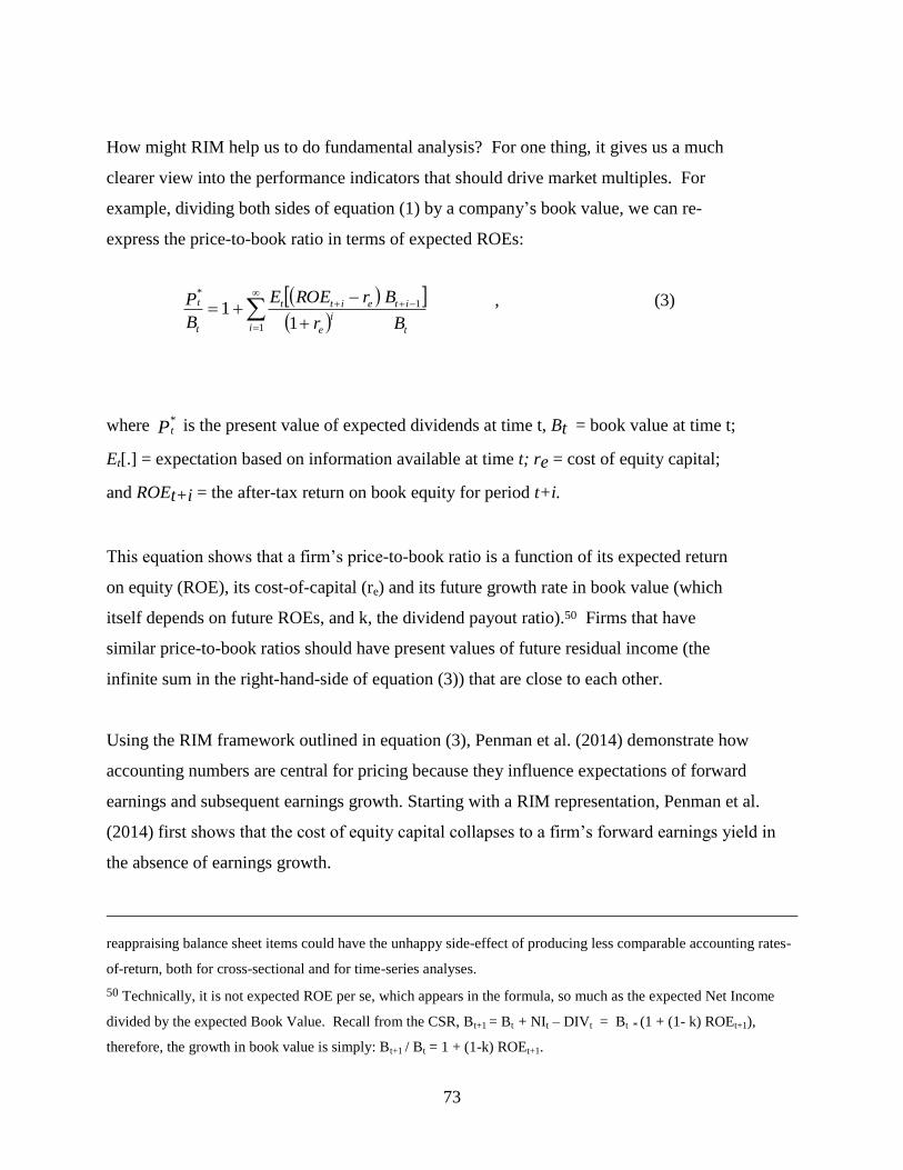
73

1

1*

11

i t

i

e

iteitt

t

t

Br

BrROEE

B

P

How might RIM help us to do fundamental analysis? For one thing, it gives us a much

clearer view into the performance indicators that should drive market multiples. For

example, dividing both sides of equation (1) by a company’s book value, we can re-

express the price-to-book ratio in terms of expected ROEs:

, (3)

where Pt* is the present value of expected dividends at time t, Bt = book value at time t;

Et[.] = expectation based on information available at time t; re = cost of equity capital;

and ROEt+i = the after-tax return on book equity for period t+i.

This equation shows that a firm’s price-to-book ratio is a function of its expected return

on equity (ROE), its cost-of-capital (re) and its future growth rate in book value (which

itself depends on future ROEs, and k, the dividend payout ratio).50 Firms that have

similar price-to-book ratios should have present values of future residual income (the

infinite sum in the right-hand-side of equation (3)) that are close to each other.

Using the RIM framework outlined in equation (3), Penman et al. (2014) demonstrate how

accounting numbers are central for pricing because they influence expectations of forward

earnings and subsequent earnings growth. Starting with a RIM representation, Penman et al.

(2014) first shows that the cost of equity capital collapses to a firm’s forward earnings yield in

the absence of earnings growth.

reappraising balance sheet items could have the unhappy side-effect of producing less comparable accounting rates-

of-return, both for cross-sectional and for time-series analyses.

50 Technically, it is not expected ROE per se, which appears in the formula, so much as the expected Net Income

divided by the expected Book Value. Recall from the CSR, Bt+1 = Bt + NIt – DIVt = Bt * (1 + (1- k) ROEt+1),

therefore, the growth in book value is simply: Bt+1 / Bt = 1 + (1-k) ROEt+1.

74

Of course, firms would be far easier to value in the absence of growth. However, the need for

more granular valuation models stem from the fact that earnings growth varies in the cross-

section. In the presence of growth, the Penman et al. (2014) framework helps illustrate that

accounting knowledge is essential for pricing because it conveys information about expected

earnings growth as well as the risks underlying these expectations. Below, we outline how

investors can leverage the RIM framework to identify value by using accounting information to

learn about the quality of a firm’s earnings potential relative (i.e., its quality) as well as the cost

of the firm relative to its assets in place (i.e., its cheapness).

3.4 The Two Sides of Value Investing

A key insight that falls directly from this analysis is that value companies are not just those that

are cheap relative to capital-in-place, but include those that are cheap relative to the present

value of their future residual income. A common misperception about value investing, at least

among academics, is that it simply involves buying stocks that are cheap relative to measures of

capital-in-place. For example, many academic studies (mostly from finance) define value stocks

as firms that trade at lower market multiples of book value, earnings, or enterprise value (e.g.,

P/B, P/E, or EV/S). Accounting-based valuation demonstrates the seriousness of this error,

because cheapness (as expressed through lower market multiples) is only one (and arguably the

much less interesting) part of value investing.

As the residual-income framework makes transparent, a firm’s true fundamental value is made

up of two key elements: Firm Value = Capital-in-place + Growth-opportunities. The

problem with typical cheapness indicators is that they only compare the price of a stock to its

capital-in-place (book value, capitalized-earnings, or sales), and miss entirely the second element

in equity valuation.

The most successful fundamental investors, beginning with Ben Graham, have always viewed

Value Investing as consisting of two key elements: (1) Finding “quality” companies, (2) Buying

them at “reasonable prices”. In simple notation:

75

Value Investing = Cheapness + Quality

A firm’s market multiple is a measure of cheapness relative to assets-in-place, but that is the

easier and arguably less interesting part of value investing. The more interesting part requires an

investor to assess a firm’s quality – that is, the present value of its expected future residual

income (PVRI), using various currently available performance indicators. That is, of course the

heart of what we call fundamental analysis. The best fundamental investors focus on buying

quality, for a given level of cheapness. It is in this spirit that Ben Graham built his original stock

screen. Looking back at his quality factors (factors #6 to 10), Graham intuitively recognized that

firms with lower leverage, higher liquidity, and a high rate of steady growth are those with the

best chance of generating high rates of return in the future. Or, in RIM parlance, he believed

these are the high PVRI stocks.

3.5 Lessons from the Field

This overarching theme of “cheapness+quality” is extremely helpful to bear in mind when trying

to understand the investment approaches of investors, such as Warren Buffett, Charlie Munger,

Joel Greenblatt, Julian Robertson, and a host of others who grew up under their tutelage (e.g., the

extremely successful “Tiger Cub” funds, such as Lone Pine, Viking, and Maverick Capital, all of

which had their roots in Julian Robertson’s Tiger Fund (1980-2000)). Let us consider one such

example.

Joel Greenblatt and the Magic Formula

Joel Greenblatt is an American academic, hedge fund manager, investor, and writer. Like

Graham, Greenblatt’s career straddled academia and Wall Street. In 1985, he founded a hedge

fund, Gotham Capital, which focused on special situation investing. Greenblatt and his

cofounder, Robert Goldstein, compounded Gotham’s capital at a phenomenal 40 percent

annually before fees for the 10 years from its formation in 1985 to its return of outside capital in

1995. After returning all outside capital, Greenblatt and Goldstein continued to invest their own

capital in special situations. In 1999, he wrote his first best-seller, You Can Be a Stock Market

Genius, which described the special situation investment strategy responsible for Gotham’s

success.

76

What Greenblatt is best known for, however, is his second book, The Little Book that Beats the

Market. Published in 2005, the first edition sold over 300,000 copies and was translated into 16

languages, thus propelling Greenblatt to celebrity-investor status. As Greenblatt described it,

this book was the product of an experiment, in which he wanted to see whether Warren Buffett’s

investment strategy could be quantified. He knew that the subtle qualitative judgment of “the

Sage from Omaha” was probably beyond the reach of machines. Still, he wondered whether

some of Buffett’s magic might be bottled.

Studying Buffett’s public pronouncements, most of which came in the form of Chairman’s letters

from Berkshire Hathaway, Inc., Greenblatt discerned a recurrent theme. As Buffett often

quipped: “It is far better to buy a wonderful company at a fair price than a fair company at a

wonderful price.”51 Buffett was not just buying cheap companies, Greenblatt observed, he was

looking for quality companies at reasonable prices. What would happen if we tried to create a

mechanical stock screen that invested in high-quality businesses trading at reasonable prices?52

The results were so impressive that in The Little Book that Beats the Market, Greenblatt called

this strategy The Magic Formula. The details of the formula are laid out in Appendix A. As you

will see from this Appendix, it is a remarkably simple strategy. Greenblatt ranked companies

based on just two factors: Return-on-capital (ROC) and earnings-yield (EY). The Magic

Formula, in a nutshell, looks for companies with a history of consistently high past ROC (5 years

of at least 20% annually), and bought the ones currently trading at the lowest earnings-yield.

That’s it!

Several points are worth noting. First, the formula works (or more precisely, it has worked for a

long time). This basic formula has been thoroughly tested using U.S. data, both by Greenblatt

51 From the Chairman’s Letter, Berkshire Hathaway, Inc., Annual Report, 1989.

52 At least one other accounting academic came to the same conclusion about Buffett’s investment strategy. In his

2010 book, Buffett beyond Value, Professor Prem Jain studied over 30 years of Buffett pronouncements and also

came to the same conclusion (Jain (2010)). Buffett favored quality growth (or in RIM parlance, high PVRI firms)

over cheapness.

77

and by others. Firms ranked at the top of this screen have outperformed their peers by a wide

margin over the past 50 years.53 Second, it is really very similar to what Ben Graham was doing

many years earlier! Five years of high and consistent growth… low P/E ratios… sounds

familiar? The more things change, the more they stay the same.

But of course, in the context of the RIM, all this makes sense. Ben Graham, Warren Buffett, and

Joel Greenblatt, they are all trying to do the same thing – find firms with high expected PVRI

trading at reasonable market multiples. Consider Buffett’s most often repeated four-fold dictum:

(1) Only invest in a business you can understand; (2) Look for companies with a sustainable

competitive advantage, (3) Bet on companies with high-quality management teams, and (4) Buy

with a good “Margin of Safety.” The last point is easiest to understand and implement – buy

firms with an attractive valuation relative to its capital base. What do the first three principles

tell us? Are they not simply pointing us towards firms with a greater likelihood of high

sustainable ROE’s in the future? The verdict from the field is clear: Quality pays.

3.6 Empirical Evidence from Academic Studies

Once we have the overarching valuation framework firmly in place, it is remarkable how well

the evidence from empirical studies line up with the theory, and with the field evidence from

investors. Let us now turn to this evidence.

Cheapness

An enormous body of literature in accounting and finance documents the tendency of value

stocks (stocks with low prices relative to their fundamentals) to outperform glamour stocks

(stocks with high prices relative to their fundamentals). Common measures of value are the

book-to-market ratio (Stattman (1980), Rosenberg, Reid, and Lanstein(1985), Fama and French

(1992)), the earnings-to-price ratio (Basu (1977), Reinganum (1981)), the cashflow-to-price ratio

(Lakonishok et al. (1994), Desai, Rajgopal, and Venkatachalam (2004)), and the sales-to-

enterprise-value ratio (O’Shaughnessy (2011)). The strength of the value effect varies over time

53 See for example, Gray and Carlisle (2013, Chapter 2) for a detailed replication of the formula using U.S. data

from 1964-2011.

78

and across stocks, but the broad tendency of value stocks to outperform glamour stocks is a

highly robust finding in the academic literature.

While academics generally agree on the empirical facts, there is much less consensus on the

reason behind these findings. Some feel the evidence clearly indicates that value stocks are

underpriced (i.e., they are bargains); others believe value stocks are cheap for a reason, and that

common measures of value are also indicators of some sort of risk. For example, Fama and

French (1992) suggest low price-to-book (P/B) stocks are more vulnerable to distress risk, and

Zhang (2005) argue that these stocks have more “trapped assets,” and are thus more susceptible

to economic downturns.54

Quality

The academic evidence in favor of quality investing has been perhaps a bit more difficult to

recognize. Up to now, academics have not always agreed on what a quality firm might look like.

Many papers have examined the persistence of earnings, for example, or the ability of

accounting-based variables to predict future returns, but most have not done so under the quality

rubric. Yet once we begin to piece together the evidence, and the composite sketch begins to fill

it, the picture that emerges bears a remarkable resemblance to the indicators of quality as first

expressed by Ben Graham in his original screen. Delightfully, the evidence also concords

extremely well with what we might expect from valuation theory.

Holding a company’s market multiple (e.g., its price-to-book ratio) constant, what kind of firm

should an investor pay more for? If we define quality firms as those that deserve a higher

multiple, then valuation theory tells us the answer. According to the RIM, quality firms are

those with a high present value of future residual income (high PVRI). The task of the empiricist

is to examine which company characteristics, or perhaps performance metrics, might serve as

useful indicators of future PVRI.

54 For a much more detailed review of this debate, see Zacks (2011; Chapter 10).

79

What are the key components of a company’s PVRI? Of first order importance would be

measures of future profitability and growth, since these elements are the primary drivers of

firms’ future ROE. Also important would be measures of safety. To the extent that safer firms

deserve a lower cost-of-capital (re), and holding future expected cash flows constant, safer firms

will deserve a higher PVRI. Finally, the expected rate of payout should play a role. Firms that

maintain the same profitability and growth rates while paying back more capital to investors are,

all else equal, deserving of a higher PVRI.

Note that we have thus far only discussed fundamental valuation, not market mispricing per se.

Superior value estimation does not always translate into better returns prediction. This is

because the latter involves a systematic mistake (some sort of error) in the current price; the

former does not. It is possible that a historical indicator of quality (such as a firm’s past ROE) is

a strong predictor of future PVRI, but the market is aware of this and has appropriately priced it.

In this case, we would not expect higher returns to an ROE-based strategy. Empirically, there

are certainly seemingly sensible value+quality combinations that do not result in superior returns

predictions. However, if prices generally converge towards fundamentals in the long run, we

should expect better valuation estimates to on average lead to superior returns prediction (see

Lee, Myers, and Swaminathan (1999) for a more detailed discussion).

Prior evidence is broadly consistent with these observations. In general, stable, safe, profitable

firms with solid growth, good cash flows, lower risk, and higher payouts do in fact earn higher

future returns. Below, we provide a brief survey of this evidence from prior research and discuss

their relation to our overarching valuation framework.

Profitability and Growth Piotroski (2000) shows that firms with better ROAs, operating cash

flows, profit margins, and asset turnovers, consistently earn higher returns. Using eight

fundamental indicators of firm performance and general health, he created a composite “F-

Score.” His evidence shows that F-Score is able to separate winners from losers from among

stocks in the lowest P/B quintile (value stocks). Mohanram (2005) performs a similar exercise

among high P/B firms (growth stocks) and find growing firms outperform firms with poor

growth. Piotroski and So (2012) use the F-Score to show the value/glamour effect is attributable

80

to errors in market expectation about future fundamentals. Using I/B/E/S analysts’ forecasts,

Frankel and Lee (1998) show that, holding P/B constant, firms with higher forecasted earnings

earn higher returns, particularly when correcting for predictable errors in the analysts’ consensus

estimates. Overall, the evidence suggests that firms with higher profitability (past or forecasted)

earn higher subsequent returns.

Earnings Quality It is not simply the quantity of earnings that matters, the quality (the expected

sustainability or persistence) of that earnings also matters. For example, Sloan (1996) and

Richardson et al. (2005) show that the cash flow component of earnings is more persistent than

the accrual component. Novy-Marx (2013) shows that Gross Margin (Sales – Cost of Goods

Sold) is an even better measure of core profits than bottom-line earnings. In this study,

profitable firms generate significantly higher returns than unprofitable firms, despite having

significantly higher valuation ratios.

Another line of research explores the usefulness of accounting numbers in identifying financial

shenanigans. Beneish (1999) estimates an earning manipulation detection model based entirely

on reported numbers from the period of alleged manipulation. In out-of-sample tests, Beneish,

Lee, and Nichols (BLN, 2013) shows this model correctly identified, in advance of public

disclosure, a large majority (71%) of the most famous accounting fraud cases that surfaced after

the model’s estimation period. Perhaps even more significantly, BLN shows that the

“probability of manipulation” (M-score) from the original Beneish model is a powerful predictor

of out-of-sample stock returns – i.e., firms that share traits with past earnings manipulators earn

lower subsequent returns after controlling for multiple other factors, including accounting

accruals.

Overall, these studies show that various accounting-based measures of cash flow profitability or

earnings quality are even better predictors of future returns than simple measures based on

reported earnings.

Safety Safer stocks earn higher returns. This result is remarkably robust across many measures

of safety. For example, lower volatility firms actually earn higher, not lower, returns

81

(Falkenstein (2012), Ang, Hodrick, Xing, and Zhang (2006)). Lower Beta firms in fact earn

higher returns (Black, Jensen, and Scholes (1972), Frazzini and Pedersen (2013)). Firms with

lower leverage earn higher returns (George and Hwang (2010), Penman et al. (2007)). Most

strikingly, firms with lower levels of financial distress also earn higher returns (Altman (1968),

Ohlson (1980), Dichev (1998), Campbell, Hilscher, and Szilagyi (2008)).55 In short, firms that

are safer, by many measures of safety, actually earn higher returns.

Put simply, firms with higher volatility, higher Beta, higher leverage, and higher bankruptcy risk

actually earn lower returns. This finding does not make sense in an equilibrium asset pricing

context – in equilibrium, firms with higher risk should be rewarded with higher future returns.

However, the result makes perfect sense if we believe that these risk measures are associated

with the discount rate markets use to compute a firm’s PVRI. Viewed in this context, safer firms

have lower cost-of-capital (re), and we would expect their PVRI (and thus their firm value) to be

higher than the riskier firms, all else equal. If the market underappreciates a firm’s true PVRI (as

we have seen in the case of firms’ Profitability and Growth indicators), then safer firms will in

fact earn higher future realized returns.56

Payout Finally, companies who make higher payouts to shareholders and creditors also earn

higher future returns. For example, companies that repurchase their shares tend to do well

(Baker and Wurgler (2002), Pontiff and Woodgate (2008), McLean, Pontiff, and Watanabe

(2009)), while firms that issue more shares tend to do worse (Loughran and Ritter (1995), Spiess

55 Both Dichev (1998) and Campbell et al. (2008) find strong evidence that distress risk is actually negatively

associated with subsequent returns. Dichev used Altman’s Z-score and Ohlson’s O-Score and show that going long

in the 70% of firms with low bankruptcy risk, and shorting the remaining 30%, yields positive returns in 12 out of 15

years (1981-1995). Campbell et al. (2008) sort stocks by into value-weighted portfolios by failure probability, and

find that average excess returns are strongly, and almost monotonically, negatively related with the probability of

failure. The safest 5% of stocks have an average excess yearly return of 3.4%, while the riskiest 1% of stocks have

an average return of -17.0%.

56 Consistent with this argument, Chava and Purnanadam (2009) show that although distress risk is negatively

correlated with future realized returns, it is positively correlated with a firm’s market-implied cost of capital. In

other words, the market does use a higher implied discount rate when discounting the future earnings of high distress

firms; however, because these firms are still over-priced on average, they still earn lower future realized returns.

82

and Affleck-Graves (1995)). A similar pattern is observed for debt issuances. Firms that issue

more debt earn negative abnormal returns (Spiess and Affleck-Graves (1999), Billett, Flannery,

and Garfinkel(2006)), while firms that retire their debt earn positive abnormal returns (Affleck-

Graves and Miller (2003)). In fact, Bradshaw et al. (2006) show that it is possible to measure

these effects using a measure of net external financing activities computed from companies’

Statement of Cash Flow. Taken together, these findings are quite consistent with the RIM

framework: firms that are returning capital at a faster rate (firms with a higher k), have more

positive PVRI.

In short, what types of firms might be deemed higher quality? In other words, which firm

characteristics are associated with higher future ROEs, lower cost-of-capital, and higher

payouts? Prior studies suggest these are safe, profitable, growing firms that are also returning

more of their capital to their investors. These facts are exactly what we would expect if markets

underappreciate fundamental value, as reflected in current financial statements. They are much

more difficult to reconcile with popular explanations of the value effect as a risk premium, as the

quality firms are more profitable, less volatile, less prone to distress, have more persistent future

cash flows, and lower levels of operating leverage.

Asness, Frazzini, and Petersen (2013)

In a fascinating new study, Asness, Frazzini, and Petersen (2013) pulls these disparate strands of

quality investing together. In this study, the authors define quality firms as stocks that are “safe,

profitable, growing, and well-managed.” They argue that all else equal investors should be

willing to pay more for such firms. They show that in fact the market does not pay a high

enough premium for these quality stocks. Sorting firms on the basis of their quality metric, they

create a “Quality Minus Junk” (QMJ) portfolio, and find that this portfolio earns positive risk-

adjusted returns in 22 out of 23 countries.

For their empirical tests, they compute a composite quality score for each firm based on the

following 21 performance indicators, grouped into four categories. Each variable is ranked, and

then normalized by subtracting its own mean and dividing by its own standard deviation:

83

I. Profitability (6 variables)

Bet in favor of firms with high earnings (ROA, ROE), high gross-profit (GPOA, GMAR) and

high operating cash flow (CFOA, ACC). The numerators are current year earnings, gross

margin, or operating cash flows; the denominators are total assets, book equity, total sales, or

(in the case of ACC) total earnings.

II. Growth (6 variables)

Bet in favor of firms with the most positive changes in these profitability variables over past

5 years (e.g., ∆GPOA = (GPt – GPt-5) / TAt-5); where GP = REV – COGS. In other words,

Asness, Frazzini, and Petersen (2013) define growth firms as those whose gross margin, or

earnings, or cash flows, have grown the most over the past five years, relative to the year t-5

capital base.

III. Safety (6 variables)

Bet against firms with Beta (BETA), high volatility in returns and earnings (IVOL, EVOL),

high leverage (LEV), and high levels of financial distress (O-score, Z-score). For this

composite, the authors consolidate six measures of “safety” based on prior studies. In

essence, safe firms are defined as those with low Beta, low volatility, low leverage, and low

financial distress.

IV. Payout (3)

Bet against firms with: high net equity issuance (EISS), high net debt issuance (DISS), low

net payout ratio (NPOP) over past five years. Again, consistent with prior studies, Asness,

Frazzini, and Petersen (2013) define high payout firms in terms of net new issuances, plus

dividends.

Notice how well these concepts map into the RIM framework. The first six indicators (past

ROE, ROA, GPOA, GMAR, CFOA, and ACC) capture profitable firms that have higher gross

margin, and a higher proportion of cash flow to accruals in their reported earnings. The next six

indicators measure improvements in these variable dimensions of profitability. In the RIM

framework, these 12 variables are all likely to be associated with higher future ROEs. Not

84

surprisingly, Asness, Frazzini, and Petersen (2013) find that these measures are strongly

correlated with P/B ratios in the cross-section.

More interestingly, Asness, Frazzini, and Petersen (2013) shows that these variables also predict

cross-sectional returns – that is, more profitable firms and firms with strong growth over the past

five years consistently earn higher returns than firms with low profitability and low growth. To

be fair, most of these variables have been reported by prior studies as being useful in returns

prediction. Nevertheless, this study provides compelling evidence in support of the prediction

from a simple RIM analysis – firms with high and persistent profits have high PVRI, and the

market does not seem to fully price in this quality metric.

The main empirical finding in Asness, Frazzini, and Petersen (2013) is that safer firms also earn

higher future returns. They define safe firms as those with lower Beta, lower volatility

(measured in terms of both idiosyncratic returns (IVOL) and past earnings (EVOL)), lower

leverage (LEV), and lower financial distress (O-Score and Z-Score). While this result might be

counter-intuitive for efficient market advocates, it is in fact quite easy to understand in terms of

the RIM framework. Holding expected cash flows constant, safer firms are worth more (i.e. they

should have lower discount rates). To the extent that markets underappreciate this dimension of

firm valuation, the safer firms would yield higher future returns.

Finally, Asness, Frazzini, and Petersen (2013) show that firms with high net payouts (i.e. those

with low net equity issuances, low debt issuances, and high dividends), are also worth more. In

the RIM framework, this is not surprising either. Firms which are able to produce the same level

of growth as other firms while paying back more of their capital to investors are worth more.

Again, when we measure the quality component of firm value (PVRI) more accurately, we are

better able to identify firms that earn higher future returns.

3.7 Why does value investing continue to work?

Two stylized facts emerge from the preceding literature survey: (a) smart value investing, which

incorporates both cheapness and quality, is associated with higher future stock returns, and (b)

these strategies are being actively exploited by professional investors. These two findings

85

naturally raise the issue of whether the value effect will persist in the future. Why haven’t these

effects been fully arbitraged away? Why does anyone continue to buy expensive, low-quality,

stocks (i.e., who buys “junk”)?

Although a full treatment of this topic is probably beyond the scope of this chapter, the academic

literature has proposed at least four reasons for the persistence of the value effect: (a) Risk-based

Explanations, (b) Preference-based Explanations, (c) Institutional- and Friction-based

Explanations and (d) Behavioral-based Explanations. We briefly review these explanations

below.

3.7.1 Risk-based Explanations

The first, and longest-standing, explanation is that value stocks are simply riskier, and

their higher future returns are a compensation for bearing this risk (e.g., Fama and French

(1992)). In support of this risk-based explanation, several studies provide evidence that value and

growth stocks possess differential sensitivities to time-varying macroeconomic risks. For

example, Vassalou (2003), Cohen, Polk, and Vuolteenaho (2009), and Santos and Veronesi

(2010) show that value stocks have greater sensitivities to economy-wide profitability than

growth stocks. Similarly, Campbell, Polk, and Vuolteenaho (2010) and Lettau and Wachter

(2007) argue that growth (value) stocks display a higher sensitivity to discount rate (cash flow)

news. Da and Warachka (2009) demonstrates that the sensitivities of firms’ cash flows to

aggregate earnings forecasts explain a significant portion of the value premium and Petkova and

Zhang (2005) finds that the value premium tends to covary positively with time-varying risk

attributes. Lastly, Zhang (2005) argues that the value premium is driven by the differential ability

of value and glamour firms to expand and contract their asset base in the face of changing

economic conditions. Taken together, these papers suggest that some, if not all, of the

documented return performance is an artifact of risk factor exposures that vary across value and

glamour firms.

Surely we can agree that value investing involves some risk – i.e., it is not a simple money pump.

This is particularly true for the naïve form of value investing commonly discussed in the

academic literature. The standard academic approach to value investing is to focus on a stock’s

86

cheapness (as measured by its market multiples). But cheap stocks (high B/M, high E/P, stocks

for example) are typically priced that way for a reason – i.e., the population of cheap stocks

contain a disproportionately large number of low-quality firms. In fact, as Piotroski (2000; Table

1) showed, the median firm in the highest B/M quintile underperforms the market by over 6%

over the next year – even though the mean return to these stocks is higher than the market.

Naïve value does involve some risk, and this is borne out in the data.

The problem with the risk-based explanation is that, properly measured, value stocks are actually

safer than the growth stocks. Once we incorporate measures of quality, it is clear that value

investing does not generally incur higher risk, on average, at least by most sensible measure of

risk (e.g., Piotroski and So (2012)). The studies surveyed earlier strongly suggest in fact stocks

with more stable cash flows, lower financial distress, lower Beta, and lower volatility, actually

earn higher future realized returns. These findings are difficult to reconcile with risk-based

explanations.

3.7.2 Preference-based Explanations

According to this explanation, some investors have a preference for stocks with “lottery-like”

payoffs – i.e. return distributions that are right-skewed. Stocks that have these features will

therefore, all else equal, appear “over-priced” in a mean-variance world (Brunnermeier and

Parker (2005) and Brunnermeier, Gollier, and Parker (2007)). Bali, Cakici, and Whitelaw (2011)

provide evidence consistent with this phenomenon, and Kumar (2005; 2009) show this effect

applies particularly to retail traders.

It seems plausible that a subset of investors might have preferences beyond the mean-variance

trade-off considered by standard asset pricing models. For example, investors may behave as if

they prefer lottery-like payoffs, however, it might be difficult to empirically separate this

explanation from some of the behavioral-based explanations below (in fact, the literature on

Information Uncertainty (Jiang, Lee, and Zhang (2005), Zhang (2005)) makes the same point in

a behavioral context). But if investors do exhibit an innate preference for lottery-like stocks, the

value effect will, of course, be likely persistence well into the future.

87

3.7.3 Institutional- and Friction-based Explanations

A. Liquidity-driven Price Pressures

Stock prices are constantly buffeted by non-fundamental price pressures. Sometimes capital

flows into or out of an asset simply “herd” in the same direction for liquidity reasons. These

provide both opportunities and challenges for value investors.

For example, in Coval and Stafford (2007): “Fire sales” by mutual funds that face redemption

pressure due to weak performance in prior quarters can depress the prices of the stocks they own

– and these stocks subsequently rebound strongly. Non-fundamental flows should reverse over

time, and may not be driven by cognitive biases. The impact of these non-fundamental price

changes are not specific to value investing, however, they will contribute to a higher return:risk

ratio for investors that trade on value indicators.

B. Prudent-Man Concerns

Del Guercio (1996) notes that institutional investors may gravitate toward glamour stocks due to

“prudent-man” concerns, which refers to the idea that investments in high profile, glamour

stocks are easier to justify as sound decisions (i.e., they make the investor appear prudent).

Skewness in institutional investors’ portfolios toward high profile firms can exacerbate the value

effect by raising demand for glamour stocks. Similarly, as noted in Green, Hand, and Soliman

(2011) and So (2013), to the extent that mispricing emerges because investors equate good

companies with good investments, glamour stocks may offer greater ex-post justifiability in case

of losses.57

57 This positive link between a firm’s profile and glamour status is also consistent with the model of capital

equilibrium under incomplete information in Merton (1987), which shows that firm value is an increasing function

of investor recognition of the firm. See Lehavy and Sloan (2018) for related evidence on the empirical link between

investor recognition and expected returns.

88

Thus, prudent-man concerns can contribute to the persistence of the value effect because

institutional investors concerned with their reputations, legal liabilities, and/or client

relationships with sponsors may fail to buy value stocks and sell glamour stocks because

potential losses may be harder to justify as prudent investments.

C. Limits to Arbitrage

Broadly speaking, the value effect may continue to exist because there are limits to arbitrage. In

finance textbooks, arbitrage is described as a riskless investment position from simultaneously

buying and selling securities, typically requiring no capital investment. This form of textbook

arbitrage is commonly referred to as ‘deterministic’ arbitrage. In practice, investors capitalize on

the value effect through ‘statistical’ arbitrage, which refers to trades based on statistical evidence

of mispricing with respect to the expected value of a given asset. Statistical arbitrage, by

contrast, entails significant risks. As noted earlier, although value investing tends to yield

positive returns, Piotroski (2000) shows that the median return to holding value firms is negative.

A related form of risk involved with statistical arbitrage is that the returns to value-based

strategies are earned over longer holding periods, which reflects the fact that underpriced value

firms tend to only gradually rise toward their expected value and overpriced glamour firms tend

to only gradually fall toward their expected value. Thus, profiting from the value effect can

require significant patience and capital deployment. Shleifer and Vishny (1997) point out that the

arbitrage mechanism is constrained because investors withdraw money from investment funds

that lose money, even if the losses result from a predictably temporary increase in mispricing.

Stocks often reach value (glamour) status in response to upward (downward) revisions in prices,

thus, a related risk in value investing is that profiting from underpriced securities may require

betting against negative momentum and vice versa for glamour stocks. Related evidence in

Brunnermeier and Nagel (2004) shows that several prominent hedge funds bet against the

internet bubble in spring 1999 and suffered significant losses and capital outflows as the bubble

continued and mispricing deepened. This example illustrates one of the central difficulties in

arbitraging the value effect: the uncertainty over when mispricing will correct. When investors’

investment horizon is short, the value effect may persist because the market lacks the sufficient

89

patience to commit the capital necessary to discipline prices. We discuss related evidence on the

limits of arbitrage in more detail in Chapter 5 of the second volume of this book.

3.7.4 Behavioral-based Explanations

The final, and in our view most intriguing, set of explanations for the value effect is rooted in

human cognitive behavior. While not mutually exclusive, we group these explanations into four

sub-categories.

A. Saliency vs. Weight

Human decision-making under uncertainty involves assessing the probability of alternative

outcomes. A recurrent theme in cognitive psychology is that human subjects consistently under-

weight the probability of certain types of events and over-weight the probability of others. In

their seminal study, Griffin and Tversky (1992) show that signals with high statistical reliability

(high “weight”) but are not salient (low “saliency”) are consistently underweighted.

Conversely, highly salient signals with low statistical reliability are often overweighted.

Apparently, Bayesian updating is a difficult cognitive task.

Apply this concept to value investing, firm attribute that are “boring” (non-salient) receive less-

than-optimal weight, and those that are “glamorous” (salient) receive more-than-optimal weight.

The historical indicators of quality discussed earlier are weighty in terms of their statistical

association with future residual income (i.e. sustainable cash flows), but they may not receive

sufficient weight in the minds of the investors. Value-based arbitrageurs help to reduce the

mispricing, but new “story stocks” arise on a daily basis as markets seek to assimilate the

constant flow of news items and/or pseudo-signals.

B. Extrapolation

A related behavioral explanation points to evidence in the psychology literature documenting the

tendency of individuals to over-extrapolate past trends (e.g., Giffin and Tversky (1992)). This

literature asserts that investors underestimate the tendency for trends in firms’ past performance

to mean revert and overestimate the tendency for them to continue. Lakonishok et al. (1994)

90

apply this insight to the pricing of stocks and provide evidence that the value effect is a result of

judgment errors where investors overestimate the persistence of past trends in firm performance

when valuing firms’ future cash flows. Related evidence in Dechow and Sloan (1996) shows that

analysts tend to fixate on past earnings growth when forecasting future earnings and that

investors tend to naively rely on analysts’ forecasts.

By overestimating the tendency of trends to continue, investors extrapolate past growth too far

leading to upwardly biased prices for glamour stocks and similarly over-extrapolate past

underperformance leading to downward biased prices for value stocks. Under this explanation,

investors place excessive weight on recent history and underweight the likelihood of mean

reversion in firms’ performance.

C. Momentum (Positive-feedback) Trading

All pure value investors face the risk that noise trading will push prices even further from

fundamental value. Value stocks tend to be negative momentum stocks – and over at least mid-

horizon (3 to 12 month) holding periods, value bets run into a momentum headwind.

Strongly negative sentiment typically accompanies really attractive buys based on fundamentals

(for recent examples, consider the risk associated with buying Greek assets, or debt instruments

issued by U.S. financial service firms, during the global crisis). Thus value inherently faces

greater short- and mid-horizon risk from positive feedback trading. The extent to which this

matters depends on the holding horizon and the stability and depth of his/her source of capital.

D. Over-confidence in high “information uncertainty” settings

Finally, the evidence is clear that firms operating in high “information uncertainty” (IU) settings

tend to earn lower subsequent returns. For example, Jiang et al. (2005) define IU in terms of

“value ambiguity,” or the precision with which firm value can be estimated by knowledgeable

investors at reasonable cost. In Jiang et al. (2005), as well as Zhang (2005), high-IU firms earn

lower future returns. In addition, high-IU firms exhibit stronger price as well as earnings

momentum effects. Specifically, younger firms, firms with higher volatility, higher volume (i.e.

turnover), greater expected growth, higher price-to-book, wider dispersion in analyst earnings

91

forecasts, and longer implied duration in future cash flows all earn lower returns. In some sense,

each of the above phenomena is related to firms’ IU measure.

Jiang et al. (2005) argues that all these observations can be traced back to the same behavioral

root: People are more overconfident in settings with high “information uncertainty”. Applied to

value investing, investors tend to overweight elements of firm value that are further out in the

future, and underweight those that are nearer at hand (in other words, they use too low an

implied discount rate when valuing firm future cash flows). This leads to a tendency to

overprice “story stocks” whose cash flows are expected further out into the future.

The overconfidence hypothesis would help to explain why strategies such as the Frankel and Lee

(1998) V/P metric (based on short-duration expected cash flows relative to stock prices) can

generate higher returns. It would also suggest an explanation for why momentum effects are

stronger in high IU settings.

3.8 Summary

Since the days of Benjamin Graham over 80 years ago, fundamental investors have served as a

stabilizing force in financial markets. In this article, we reviewed the theoretical foundations of

this style of investing including an accounting-based valuation framework for reconciling the

vast empirical evidence. We have also attempted to reconcile the investment approaches of

some well-known fundamental investors with recent findings from academia.

A number of recent studies provide compelling evidence that historical accounting numbers are

informative, and are already playing a useful role in fundamental investing. For example, none

of the 21 indicators in the composite quality index featured in Asness, Frazzini, and Petersen

(2013) rely on a company’s stock price. They are all variable constructed from historical GAAP-

based financial statements. Yet together these variables provide a good composite sketch of

companies that tend to earn higher returns in the future.

The RIM helps us to understand why. Careful fundamental analysis can help us to derive

performance measures that help predict the future profitability and growth of firms. It can also

92

help us assess the riskiness of a firm, as well as its likely future payout to shareholders. In short,

accounting information can help us to evaluate not only the first moment of a firm’s future cash

flows (i.e., the numerator of the future payoffs), but also its second moment (i.e., the riskiness of

these payoffs). As valuation theory shows, both elements are useful in evaluating the present

value of a firm’s future growth opportunities. In fact, the key predictions from valuation theory

dovetail nicely, not only with recent empirical findings in academia, but also with the age-old

wisdom espoused by many savvy investors.

We might not be there yet, but we are good ways down the road mapped out for us by Ben

Graham almost 80 years ago. The verdict from the field agrees with the verdict from the ivory

tower. Buy quality firms at reasonable prices, and use historical accounting numbers to help you

achieve that task. It will give you an edge in your investing, and help make markets more

efficient as well!

93

References

Altman, E., 1969, Financial ratios, discriminant analysis and the prediction of corporate

bankruptcy, Journal of Finance 23, 589-609.

Affleck-Graves, J., and R. Miller, 2003, The information content of calls of debt: evidence from

long-run stock returns, Journal of Financial Research 26, 421-447.

Ang, A., R. Hodrick, Y. Xing, X. Zhang, 2006, The cross-section of volatility and expected

returns, Journal of Finance 61, 259-299.

Arif, S., and C. M. C. Lee, 2014, Aggregate investment and investor sentiment, Review of

Financial Studies, forthcoming.

Asness, C. S., A. Frazzini, and L. H. Pedersen, 2013, Quality minus junk, AQR Capital

Management and New York University working paper, October 9.

Baker, M., and J. Wurgler, 2002, Market timing and capital structure, Journal of Finance 57, 1-

32.

_________________, 2007, Investor Sentiment in the stock market, Journal of Economic

Perspectives 21, 129-151.

Basu, S., 1977, The Investment Performance of Common Stocks in Relation to Their Price-to-

Earnings: A Test of the Efficient Markets Hypothesis, Journal of Finance 32, 663-682.

Beneish, D., 1999, The detection of earnings manipulation, Financial Analysts Journal 55:5, 24-

36.

Beneish, D., C. M. C. Lee, and C. Nichols, 2013, Earnings manipulation and expected returns,

Financial Analysts Journal 69:2, 57-82.

Bernard, V. L., 1995, The Feltham-Ohlson framework: implications for empiricists,

Contemporary Accounting Research 11, 733-747.

Bhojraj, S., and C. M. C. Lee, 2002, Who is my peer? A valuation-based approach to the

selection of comparable firms, Journal of Accounting Research 40, 407-439.

Billett, M., M. Flannery, and J. Garfinkel, 2006, Are bank loans special? Evidence on the post-

announcement performance of bank borrowers, Journal of Financial and Quantitative

Analysis 41, 733-751.

94

Black, F., 1986, Noise, from the papers and proceedings of the forty-fourth annual meeting of the

American Finance Association, Journal of Finance 41, 529-543.

Black, F., M. C. Jensen, and M. Scholes, 1972, The Capital Asset Pricing Model: Some

Empirical Tests, in Michael C. Jensen (ed.), Studies in the Theory of Capital Markets, New

York, 79-121.

Bradshaw, M., S. Richardson, and R. Sloan, 2006, The relation between corporate financing

activities, analysts’ forecasts and stock returns, Journal of Accounting and Economics 42,

53-85.

Brunnermeier M. K. and S. Nagel, 2004, Hedge funds and the technology bubble, Journal of

Finance 59, 2013-2040.

Campbell, J., J. Hilscher, and J. Szilagyi, 2008, In search of distress risk, Journal of Finance 63,

2899-2939.

Campbell, J., C. Polk, and T. Vuolteenaho. 2010. Growth or Glamour? Fundamentals and

Systematic Risk in Stock Returns. Review of Financial Studies 23, 306-344.

Campbell, J., and R. J. Shiller, 1988, The dividend-price ratio and expectations of future

dividends and discount factors, Review of Financial Studies 1:3, 195-228.

Chava, S., and A. Purnanadam. 2009. Is default risk negatively related to stock returns? Review

of Financial Studies, forthcoming.

Cottle, S., R. F. Murray, and F. E. Block, 1988, Graham and Dodd’s Security Analysis, Fifth

Edition, McGraw-Hill Book Company.

Coval J., and E. Stafford, 2007, Asset fire sales (and purchases) in equity markets. Journal of

Financial Economics 86, 479-512.

Cutler, D., J. Poterba, and L. Summers, 1989, What moves stock prices? Journal of Portfolio

Management, Spring, 4-12.

Da, Z. and M. Warachka. 2009. Cashflow risk, systematic earnings revisions, and the cross-

section of stock returns, Journal of Financial Economics 94, 448-468.

95

Damodaran, A., 2012, Value investing: Investing for grown ups? Stern School of Business,

NYU working paper, April.

Dechow, P. M., & Sloan, R. G., 1997, Returns to contrarian investment strategies: Tests of naive

expectations hypotheses. Journal of Financial Economics, 43(1), 3-27.

Del Guercio, D. (1996). The distorting effect of the prudent-man laws on institutional equity

investments. Journal of Financial Economics, 40(1), 31-62.

Desai, H., S. Rajgopal, and M. Venkatachalam, 2004, Value-Glamour and Accrual-based Market

Anomalies: One Anomaly or Two? The Accounting Review 79, 355-385.

Dichev, I., 1998, Is the risk of bankruptcy a systematic risk? Journal of Finance 53, 1131-1147.

Easton, P., 2004, PE Ratios, PEG Ratios, and Estimating the Implied Expected Rate of Return on

Equity Capital, The Accounting Review 79, 73–96.

Edwards, E. O., and P. W. Bell, 1961, The Theory and Measurement of Business Income,

University of California Press, Berkeley, CA.

Falkenstein, Eric G., 2012, The missing risk premium: why low volatility investing works, Eric G.

Falkenstein.

Fama, E. F., and K. R. French, 1992, The cross-section of expected stock returns, Journal of

Finance 47, 427-465.

Feltham, G. A., and J. A. Ohlson, 1995, Valuation and clean surplus accounting for operating

and financial activities, Contemporary Accounting Research 11, 689-731.

FASB (Financial Accounting Standards Board), 1978, Statement of Financial Accounting

Concept No. 1, November.

Frankel, R., and C. M. C. Lee, 1998, Accounting valuation, market expectation, and cross-

sectional stock returns, Journal of Accounting and Economics 25, 283-319.

Frazzini, A., and L. H. Pedersen, 2013, Betting Against Beta, Journal of Financial Economics,

forthcoming.

96

George, T. J., and C. Y. Hwang, 2010, A resolution of the distress risk and leverage puzzles in

the cross section of stock returns, Journal of Financial Economics 96, 56-79.

Graham, B., and D. Dodd, 1934, Security Analysis: Principles and Techniques, 1st Edition, New

York and London, McGraw-Hill,

Gray, W. R., and T. E. Carlisle, 2013, Quantitative value: a practitioner’s guide to automating

intelligent investment and eliminating behavioral errors, Wiley and Sons, Hoboken, New

Jersey.

Green, J., Hand, J. R., & Soliman, M. T., 2011, Going, going, gone? The apparent demise of the

accruals anomaly. Management Science, 57(5), 797-816.

Greenblatt, J., 2010, The little book that still beats the market, John Wiley and Sons, Hoboken,

NJ.

Griffin, D., and Tversky, A., 1992, The weighing of evidence and the determinants of

confidence. Cognitive psychology, 24(3), 411-435.

Healy, P. M., and K. G. Palepu, 2012, Business analysis and valuation: using financial

statements, 5th

Edition, Cengage Learning.

Hirshleifer, D., 2001, Investor psychology and asset pricing, Journal of Finance 56, 1533-1597.

Hirshleifer, D., S. S. Lim, and S. H. Teoh, 2009, Driven to distraction: Extraneous events and

underreaction to earnings news, Journal of Finance 64, 2289-2325.

Jain, P. C., 2010, Buffett beyond value: why Warren Buffett looks to growth and management

when investing, John Wiley and Sons, Hoboken, NJ.

Jensen, M. C., 1978, Some anomalous evidence regarding market efficiency, Journal of

Financial Economics 6, 95-101.

97

Jiang, G., Lee, C. M., & Zhang, Y., 2005, Information uncertainty and expected returns, Review

of Accounting Studies, 10(2-3), 185-221.

Kumar, A., and C. M. C. Lee, 2006. Retail investor sentiment and return comovements,

Journal of Finance 61, 2451-2486.

Lakonishok, J., A. Shleifer, and R. W. Vishny, 1994, Contrarian investment, extrapolation, and

risk, Journal of Finance 49, 1541-1578.

Lang, M., & Lundholm, R. (1996). The Relation Between Security Returns, Firm Earnings, and

Industry Earnings. Contemporary Accounting Research, 13(2), 607-629.

Lettau, M. and J. Wachter. 2007. Why Is Long-Horizon Equity Less Risky? A Duration-Based

Explanation of the Value Premium. Journal of Finance 62, 55-92.

Lee, C. M. C., 1999, Accounting-based valuation: Impact on business practices and research,

Accounting Horizons 13(4), 413-425.

, 2001, Market efficiency and accounting research, Journal of Accounting and

Economics 31, 233-253.

Lee, C., Myers, J., and B. Swaminathan, 1999, What is the intrinsic value of the Dow? Journal of

Finance 54, 1693-1741.

Lee, C. M. C., A. Shleifer and R. Thaler, 1991, Investor sentiment and the closed-end fund

puzzle, Journal of Finance 46, 75-109.

Lehavy, R., & Sloan, R. G. (2008). Investor recognition and stock returns. Review of Accounting

Studies, 13(2-3), 327-361.

Lehman, B., 1993, Earnings, dividend policy, and present value relations: Building blocks of

dividend policy invariant cash flows, Review of Quantitative Finance and Accounting 3,

263-282.

Lundholm, R., 1995, A tutorial on the Ohlson and Feltham/Ohlson Models: Answers to some

frequently-asked questions, Contemporary Accounting Research 11, 749-762.

Loughran, T., and J. Ritter, 1995, The new issues puzzle, Journal of Finance 50, 23-51.

McLean, D., J. Pontiff, and A. Watanabe, 2009, Share issuance and cross-sectional returns:

international evidence, Journal of Financial Economics 94, 1-17.

98

Merton, R. C. (1987). A simple model of capital market equilibrium with incomplete

information. Journal of Finance, 42(3), 483-510.

Mohanram, P., 2005, Separating winners from losers among low book-to-market stocks using

financial statement analysis, Review of Accounting Studies 10, 133-170.

Novy-Marx, R., 2013, The other side of value: the gross profitability premium, Journal of

Financial Economics 108, 1-28.

Ohlson, J. A., 1980, Financial ratios and the probabilistic prediction of bankruptcy, Journal of

Accounting Research 18, 109-131.

, 1990, A synthesis of security valuation theory and the role of dividends, cash

flows, and earnings, Contemporary Accounting Research 6, 648-676.

, 1991, The theory of value and earnings, and an introduction to the Ball-

Brown analysis, Contemporary Accounting Research 7, 1-19.

, 1995, Earnings, book values, and dividends in security valuation,

Contemporary Accounting Research 11, 661-687.

Ohlson, J. A., and B. Juettner-Nauroth, 2005, “Expected EPS and EPS Growth as Determinants

of Value,” Review of Accounting Studies 10, 349-365.

O’Shaughnessy, J. P., 2011, What works on Wall Street, Fourth Edition, McGraw-Hill.

Peasnell, K., 1982, Some formal connections between economic values and yields and

accounting numbers, Journal of Business Finance and Accounting 9, 361-381.

Penman, S. H., 1991, An Evaluation of Accounting Rate-of-return, Journal of Accounting,

Auditing, and Finance 6, 233-255.

, 1996, The articulation of price-earnings ratios and market-to-book ratios and

the evaluation of growth, Journal of Accounting Research 34, 235-259.

, 1997, A synthesis of equity valuation techniques and the terminal value

calculation for the dividend discount model, Review of Accounting Studies 2, 303-323.

, 2010, Accounting for value, Columbia University Press.

, 2012, Financial statement analysis and security valuation, Fifth Edition,

McGraw-Hill/Irwin.

99

Penman, S.H., F. Reggiani, S. Richardson, and I. Tuna, 2014, An Accounting-Based

Characteristic Model for Asset Pricing, working paper, Columbia University, Bocconi

University, and London Business School, May.

Penman, S. H., S. Richardson, and I. Tuna, 2007, The book-to-price effect in stock returns:

accounting for leverage, Journal of Accounting Research 45, 427-467.

Petkova, R. and L. Zhang. 2005. Is value riskier than growth? Journal of Financial Economics

78 (1), 187-202.

Piotroski, J., 2000, Value investing: the use of historical financial statement information to

separate winners from losers, Journal of Accounting Research 38, 1-41.

Piotroski J., and E. So, 2012, Identifying expectation errors in value/glamour strategies: a

fundamental analysis approach, Review of Financial Studies 25, 2841-2875.

Pontiff, J., and W. Woodgate, 2008, Share issuance and cross-sectional returns, Journal of

Finance 63, 921-945.

Preinreich, Gabriel, 1938, Annual survey of economic theory: The theory of depreciation,

Econometrica 6, 219-241.

Reinganum, M. R., 1981, Misspecification of capital asset pricing: Empirical anomalies based on

earnings’ yield and market values, Journal of Financial Economics 9, 19-46.

Richardson, S., R. G. Sloan, M. Soliman, and I. Tuna, 2005, Accrual reliability, earnings

persistence, and stock prices, Journal of Accounting and Economics 39, 437-485.

Richardson, S., R. Sloan, and H. You, 2012, What makes stock prices move? Fundamentals vs

investor recognition. Financial Analysts Journal 68:2, 30-50.

Roll, R., 1984, Orange Juice and Weather, American Economic Review 74, 861-880.

Rosenberg, B., K. Reid, and R. Lanstein, 1985, Persuasive evidence of market inefficiency,

Journal of Portfolio Management 11, 9-17.

Shiller, R. J., 1981, Do stock prices move too much to be justified by subsequent changes in

dividends?, American Economic Review 71, 421-436.

Shiller, R. J., 1984, Stock prices and social dynamics, The Brookings Papers on Economic

Activity 2, 457-510.

Shleifer, A., and R. W. Vishny, 1997, The limits of arbitrage, Journal of Finance 52, 35-55.

100

Sloan, R. G., 1996, Do stock prices fully reflect information in accruals and cash flows about

future earnings? The Accounting Review 71, 289-315.

So, E. C., 2013, A new approach to predicting analyst forecast errors: Do investors overweight

analyst forecasts?. Journal of Financial Economics, 108(3), 615-640.

Spiess, K., and J. Affleck-Graves, 1995, Underperformance in long-run stock returns following

seasoned equity offerings, Journal of Financial Economics 38, 243-267.

, 1999, The long-run performance of stock returns after debt offerings,

Journal of Financial Economics 54, 45-73.

Stattman, D., 1980, Book values and stock returns, The Chicago MBA: A Journal of Selected

Papers 4: 25-45.

Summers, L. H., 1986, Does the stock market rationally reflect fundamental values? Journal of

Finance 41:3, 591-601.

Tversky, A., & Kahneman, D., 1974, Judgment under uncertainty: Heuristics and biases. science,

185(4157), 1124-1131.

Vassalou, M., 2003. News related to future GDP growth as a risk factor in equity returns.

Journal of Financial Economics 68, 47-73.

Wahlen, J. M., S. P. Baginski, and M. Bradshaw, 2010, Financial reporting, financial statement

analysis and valuation: a strategic perspective, 7th

Edition, Cengage Learning.

Zacks, L., (ed.), 2011, The Handbook of Equity Market Anomalies: Translating Market

Inefficiencies into Effective Investment Strategies, Wiley & Sons.

Zhang, L., 2005, The value premium, Journal of Finance 60, 67-103.

101

Appendix A

Joel Greenblatt’s Magic Formula

The following basic instructions for the Magic Formula are extracted from The Little Book that

Still Beats the Market, written by Joel Greenblatt and published in 2010. They are included here

for illustrative purposes. Interested readers are encouraged to either buy the book or visit

Greenblatt’s website: magicformulainvesting.com for more details.

Greenblatt’s Basic Principle:

• Buy good businesses (high return on capital) at bargain prices (high earnings yield).

• Do this consistently by maintaining a portfolio of 20 to 30 stocks, and spreading out the

timing of your purchases (buy a few stocks each month throughout the year).

• Hold the winners for at least one year (for tax efficiency reasons).

Implementing Greenblatt’s “Magic Formula”

• Look for companies with an average ROC of 20% or higher over the past 5-years (see

below for details on ROC calculation).

• Among these, pick those ones with the highest earnings-yield (EY).

• Limit stocks to those with at least $200m in Market Cap; Exclude Utilities; Financials;

ADRs; and firms that have reported earnings within the past week.

• Also consider excluding firms with and earnings yield in excess of 20% (which may

indicate a data problem or an unusual situation).

Detailed Factor Definitions:

• Return-on-Capital (ROC) = EBIT / Capital

Where EBIT is Earnings before interest and taxes, and Capital is defined as: Net PP&E +

Net Working Capital.

102

• Earnings Yield (EY) = EBIT / TEV

Where EBIT is Earnings before interest and taxes, and TEV is defined as: Market

capitalization + total debt – excess cash + preferred stock + minority interests (excess

cash is cash + current assets – current liabilities).

Figure 1. Portfolio Returns for the Levin-Graham Stock Screen

Test Period o1/02/1999 to 11/13/2103

This figure depicts the results of a backtest conducted using a sample of U.S. companies over the

1/2/1999 to 11/9/2013 time period. At the beginning of each quarter, firms are sorted into 10

portfolios according to their Levin-Graham score (based on the original Ben Graham stock

screen described in the text). A firm is assign a +1 score if it meets each condition in the screen;

top firms can receive a maximum score of 10, bottom firms can score as low as 0. This figure

depicts the equal-weighted return to each of these 10 portfolios over the next three months

(annualized, assuming quarterly rebalancing). The left-most column is the return to the S&P400

Midcap (value-weighted) index over the same time period. All variables are computed using

publicly available data as of portfolio formation, and all firms with available Compustat and

C R S P d a t a a n d a s t o c k p r i c e o f $ 3 o r m o r e a r e i n c l u d e d .

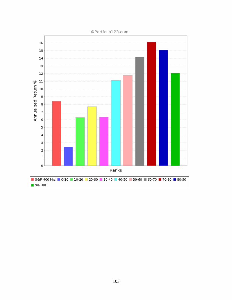
103