Machine Vision and Applications (2018) 29:299–311https://doi.org/10.1007/s00138-017-0889-4

ORIGINAL PAPER

Almost constant-time 3D nearest-neighbor lookup using implicitoctrees

Bertram H. Drost1 · Slobodan Ilic2

Received: 27 October 2016 / Revised: 22 August 2017 / Accepted: 20 October 2017 / Published online: 12 December 2017© The Author(s) 2017. This article is an open access publication

Abstract Arecurring problem in 3Dapplications is nearest-neighbor lookups in 3D point clouds. In this work, a novelmethod for exact and approximate 3D nearest-neighborlookups is proposed that allows lookup times that are, con-trary to previous approaches, nearly independent of thedistribution of data and query points, allowing to use themethod in real-time scenarios. The lookup times of the pro-posed method outperform prior art sometimes by severalorders of magnitude. This speedup is bought at the priceof increased costs for creating the indexing structure, which,however, can typically be done in an offline phase. Addi-tionally, an approximate variant of the method is proposedthat significantly reduces the time required for data structurecreation and further improves lookup times, outperformingall other methods and yielding almost constant lookup times.The method is based on a recursive spatial subdivision usingan octree that uses the underlying Voronoi tessellation assplitting criteria, thus avoiding potentially expensive back-tracking. The resulting octree is represented implicitly usinga hash table, which allows finding the leaf node a query pointbelongs to with a runtime that is logarithmic in the tree depth.The method is also trivially extendable to 2D nearest neigh-bor lookups.

Keywords Nearest neighbors · Voronoi cells · 3D pointcloud processing

B Bertram H. Drostdrost@mvtec.com

Slobodan IlicSlobodan.Ilic@siemens.com

1 MVTec Software GmbH, Arnulfstr. 205, 80634 Munich,Germany

2 Siemens AG, Otto-Hahn-Ring 6, 81739 Munich, Germany

Mathematics Subject Classification 65D19

1 Introduction and overview

Quickly finding the point closest to some query point from alarge set of data points in 3D is crucial for alignment algo-rithms, such as ICP [4], as well as industrial inspection androbotic navigation tasks. Most state-of-the-art methods forsolving the nearest-neighbor problem in 3D are based onrecursive subdivisions of the underlying space to form atree of volumes. The various subdivision strategies includeuniform subdivisions, such as octrees [21], as well as nonuni-form subdivisions, such as k-d-trees [3] and Delaunay- orVoronoi-based subdivisions [10].

Tree-based methods require two steps to find the exactnearest neighbor. First, the query point descends the tree tofind its corresponding leaf node. Since the query point mightbe closer to the boundary of the node’s volume than to thedata points contained in the leaf node, tree backtracking isrequired as a second step to search neighboring volumes forthe closest data point.

The proposed method improves on both steps: the timefor finding the leaf node is reduced by using a regularoctree that is implicitly stored in a hash table, and the needfor backtracking is eliminated by building the octree uponthe Voronoi tessellation. The leaf voxel that contains thequery point is found by bisecting the voxel level. For treesof depth L , this approach requires only O(log(L)) opera-tions, instead of O(L) operations when letting the querypoint descend the tree. In addition, each voxel contains alist of all data points whose Voronoi cells intersect thatvoxel, such that no backtracking is necessary. By storing thevoxels in a hash table and enforcing a limit on the num-ber of Voronoi intersections per voxel, the total query time

123

300 B. H. Drost, S. Ilic

is independent of the position of the query point and thedistribution of data points. The query time is of magnitudeO(log(log(N )), where N is the size of the target data pointset.

The amount of backtracking that is required in tree-basedmethods depends on the position of the query point. Meth-ods based on backtracking therefore have non-constant querytimes, making them difficult to use in real-time applications.Since the proposed method does not require backtracking,the query time becomes almost independent of the positionof the query point. Further, the method is largely parameterfree, does not require an a-priori definition of a maximumquery range, and is straightforward and easy to imple-ment.

We evaluate the proposed method on different syntheticdatasets that showdifferent distributions of the data andquerypoint sets, and compare it to several state-of-the-art methods:a self-implemented k-d-tree, theApproximate Nearest neigh-bor (ANN) library [22] (which, contrary to its name, allowsalso to search for exact nearest neighbors), the Fast Libraryfor Approximate Nearest Neighbors (FLANN) [23], and theExtremely Fast Approximate Nearest-Neighbor search Algo-rithm (EFANNA) [15] framework. The experiments showthat the proposed method is significantly faster for largerdata sets and shows an improved asymptotic behavior. As atrade-off, the proposed method uses a more expensive pre-processing step.

We also evaluate an extension of the method that per-forms approximate nearest-neighbor lookups, which is fasterfor both the preprocessing and the lookup steps. Finally,we demonstrate the performance of the proposed methodwithin two applications on real-world datasets, pose refine-ment and surface inspection. The runtime of both appli-cations is dominated by the nearest-neighbor lookups,which is why both greatly benefit from the proposedmethod.

2 Related work

Anextensive overviewover different nearest-neighbor searchstrategies can be found in [25]. Nearest-neighbor searchstrategies can roughly be divided into tree-based and hash-based approaches. Concerning tree-based methods, vari-ants of the k-d-tree [3] are state-of-the-art for applica-tions such as ICP, navigation and surface inspection [14].For high-dimensional datasets, such as images or imagedescriptors, embeddings into lower-dimensional spaces aresometimes used to reduce the complexity of the prob-lem [20].

Many methods were proposed for improving the nearest-neighbor query time by allowing small errors in the computedclosest point, i.e., by solving the approximate nearest-

neighbor problem [1,8,18]. While faster, using approxi-mations changes the nature of the lookup and is onlyapplicable for methods such as ICP, where a small numberof incorrect correspondences can be dealt with statistically.Fu and Cai [15] build a graph between nearest neigh-bors, allowing them to find approximate nearest neighborsusing a graph search. Given a potential nearest neigh-bor, its neighbors are evaluated on the the neighbor ofmy neighbor might be my neighbor premise. This leads tohighly efficient queries in higher dimensions, at the costof preprocessing time. The iterative nature of ICP canbe used to accelerate subsequent nearest-neighbor lookupsthrough caching [17,24]. Such approaches are, however,only usable for ICP and not for defect detection or othertasks.

Yan and Bowyer [26] proposed a regular 3D grid of voxelsthat allow constant-time lookup for a closest point, by storinga single closest point per voxel. However, such fixed-sizevoxel grids use excessive amounts of memory and require atrade-off between memory consumption and lookup speed.The proposed multi-level adaptive voxel grid overcomes thisproblem, since more and smaller voxels are created only atthe interesting parts of the data point cloud, while the speedadvantage of hashing is mostly preserved. Glassner [9,16]proposed to use a hash table for accessing octrees, which isthe basis for the proposed approach.

Using Voronoi cells is a natural way to approach the near-est neighbor problem, since a query point is always containedin the Voronoi cell of its nearest neighbor. Boada et al [7]proposed an octree that approximates generalized Voronoicells and that can be used to approximately solve the nearest-neighbor problem [6]. Their work also gives insight into theconstruction costs of such an octree. Contrary to the pro-posed algorithm, their work concentrates on the constructionof the data structure and solves the nearest-neighbor prob-lem only approximately. Additionally, their proposed octreestill requires O(depth) operations for a query, for an octreeof average depth depth. However, their work indicates howthe proposed method can be generalized to other metricsand to shapes other than points. Similarly, Har-Peled [19]proposed an octree-like approximation of the Voronoi tessel-lation. Birn et al [5] proposed a full hierarchy of Delaunaytriangulations for 2Dnearest-neighbor lookups.However, theauthors state that their approaches are unlikely to work wellin 3D and beyond.

Thiswork extends our previouswork [11],whichdescribesthe hash-implicit octree search. This paper additionallyincludes

– an approximate nearest-neighbor variant of the method;– additional theoretical discussions regarding failure cases,search complexity, and extensions to higher dimensions;

– experiments regarding the influence of the different steps;

123

Almost constant-time 3D nearest-neighbor lookup using implicit octrees 301

– comparisons to more related work, including FLANNand EFANNA.

3 Exact search

3.1 Notation and overview

We denote points from the target data set as x ∈ D and pointsof the query set q ∈ Q. D contains N = |D| points. Given aquery point q, the objective is to find a closest point

NN(q, D) = arg minx∈D

|q − x|2. (1)

The individual Voronoi cells of the Voronoi diagram of Dare denoted voro(x), which we see as closed set. Table 1summarizes the notations.

Note that the nearest neighbor of q in D is not necessarilyunique, since multiple points in D can have the same dis-tance to q. In many practical applications of this method,however, we are mostly interested in a single nearest neigh-bor. Additionally, considering rounding errors and floatingpoint accuracy, it is highly unlikely for a measured point toactually have multiple nearest neighbors in practice. We willtherefore talk of the nearest neighbor, even though this istechnically incorrect.

The proposed method requires a pre-processing stepwhere the voxel hash structure for the data set D is cre-ated. Once this data structure is precomputed, it remainsunchanged and can be used for subsequent queries. Thecreation of the data structure is done in three steps: The com-putation of the Voronoi cells for the data set D, the creation

Table 1 Summary of notations used in this work

Notation Description

D ⊂ R3 Target point cloud

N = |D| Size of target point cloud

NN(q, D) Nearest neighbor of q ∈ R3 in D

ANN(q, D) Approximate nearest neighbor

voro(x) Voronoi cell of x in D: voro(x) = {y ∈ R3 :

∀x̂ ∈ D : |y − x| ≤ |y − x̂|}.v ⊂ R

3 A voxel in 3D space

l(v) Voxel level

L(D, v) Set of all data points whose Voronoi cellintersects with voxel v

Mmax Maximum list length

Lmax Maximum voxel level

vol(V ) Volume of V ⊂ R3

diam(V ) Maximum diameter of V ⊂ R3:

diam(V ) = max{|x − y| : x, y ∈ V }

Fig. 1 Toy examples in 2D of the creation of the hierarchical voxelstructure. For the data point set (left), the Voronoi cells are computed(center). Starting with the root voxel that encloses all points, voxelsare recursively split if the number of intersecting Voronoi cells exceedsMmax. In this example, the root voxel is split until each voxel intersectsat most Mmax = 5 Voronoi cells (right)

of the octree and the transformation of the octree into a hashtable.

3.2 Octree creation

Using Voronoi cells is a natural way to approach the nearestneighbor problem.Aquerypointq is always containedwithinthe Voronoi cell of its closest point, i.e.,

q ∈ voro(NN(q, D)). (2)

Thus, finding a Voronoi cell that contains q is equivalentto finding NN(q, D). However, the irregular and data-dependent structure of the Voronoi tessellation does notallow a direct lookup. To overcome this, we use an octreeto create a more regular structure on top of the Voronoi dia-gram, which allows to find the corresponding Voronoi cellquickly.

After computing the Voronoi cells for the data set D, anoctree is created, whose root voxel contains the expectedquery range. Note that the root voxel can be several thousandtimes larger than the extend of the data set without significantperformance implications.

Contrary to traditional octrees, where voxels are splitbased on the number of contained data points, we split eachvoxel based on the number of intersectingVoronoi cells: Eachvoxel that intersects more than Mmax Voronoi cells is splitinto eight sub-voxels, which are processed recursively. Fig-ure 1 shows a 2D example of this splitting. The set of datapoints whose Voronoi cells intersect a voxel v is denoted

L(D, v) = {x ∈ D : voro(x) ∩ v �= ∅}. (3)

123

302 B. H. Drost, S. Ilic

This splitting criterion allows a constant processing timeduring the query phase: For any query point q containedin a leaf voxel vleaf , the Voronoi cell of the closest pointNN(q, D) must intersect vleaf . Therefore, once the leaf nodevoxel that contains q is found, at most Mmax data points mustbe searched for the closest point. The given splitting criterionthus removes the requirement for backtracking.

The cost for this is a deeper tree, since a voxel typicallyintersectsmoreVoronoi cells than it contains data points. Theirregularity of the Voronoi tessellation and possible degen-erated cases, as discussed below, make it difficult to givetheoretical boundson thedepthof the octree.However, exper-imental validation shows that the number of created voxelsscales linearly with the number of data points |D| (see Fig. 6,Left).

3.3 Hash table

The result of the recursive subdivision is an octree, asdepicted in Fig. 1. To find the closest point of a given querypoint q, two steps are required: find the leaf voxel vleaf(q)

that contains q and search all points in L(D, vleaf(q)) forthe closest point of q. The computation costs for finding theleaf node in an octree with average depth depth are on aver-age O(depth) ≈ O(log(|D|)) when letting q descend thetree in a conventional way. We propose to use the regular-ity of the octree to reduce these costs to O(log(depth)) ≈O(log(log(|D|))). For this, all voxels of the octree are storedin a hash table that is indexed by the voxel’s level l(v) andthe voxel’s integer-valued coordinates idx(v) ∈ Z

3 (Fig. 2).The leaf voxel vleaf(q) is then found by bisecting its level.

The minimum and maximum voxel level is initialized aslmin = 1 and lmax = depth. The existence of the voxel withthe center level lc = (lmin+lmax)/2� is tested using the hashtable. If the voxel exists, the search proceeds with the inter-

Level

1

23

45

67

89

Hash Table

(l = 9, idx1)

(l = 5, idx2)

(l = 3, idx3)

Fig. 2 The hash table stores all voxels v, which are indexed throughtheir level l and their index idx that contains the integer-valued coordi-nates of the voxel. The hash table allows to check for the existence of avoxel in constant time

l1 = 5

l3 = 6

l2 = 7

Fig. 3 Toy example in 2D of how to find the leaf voxel by bisecting itslevel. Finding the leaf node by letting the query point descend the treewould require O(depth) operations on average, for an octree of depthdepth (green path). Instead, the leaf node is found through bisection ofits level. In each step, the hash table is used to check for the presence ofthe corresponding voxel. The search starts with the center level l1 = 5and, since the voxel exists, proceeds with l2 = 7. Since the voxel atlevel l2 does not exist, level l3 = 6 is checked and the leaf node isfound. This requires only three lookups, compared to 6 lookups in thegreen path (color figure online)

val [lc, lmax]. Otherwise, it proceeds to search the interval[lmin, lc−1]. The search continues until the interval containsonly one level, which is the level of the leaf voxel vleaf(q).Figure 3 illustrates this bisection on a toy example .

Note that in our experiments, tree depths were in the orderof 20–40 such that the expected speedup over the traditionalmethod was around 5. Additionally, each voxel in the hashtable contains the minimum and maximum depth of its sub-tree to speedup the bisection. Additionally, the lists L(D, v)

are stored only for the leaf nodes. The primary cost duringthe bisection are cache misses when accessing the hash table.Therefore, an inlined hash table is used to reduce the averageamount of cache misses.

3.4 Runtime complexity

The runtime complexity of the different steps for finding anearest neighbor NN(q, D) in a set of N = |D| points canbe estimated as follows:

– Empirically, the depth of the octree is depth = O(N )

(see Sect. 5.1)– Using the bisection search, the leaf voxel v of q can be

found in O(log(depth)) = O(log(log(N )))

– Since the number of points contained in the leaf voxel isbound by Mmax, finding the closest point to q from thatlist can be done in O(1).

123

Almost constant-time 3D nearest-neighbor lookup using implicit octrees 303

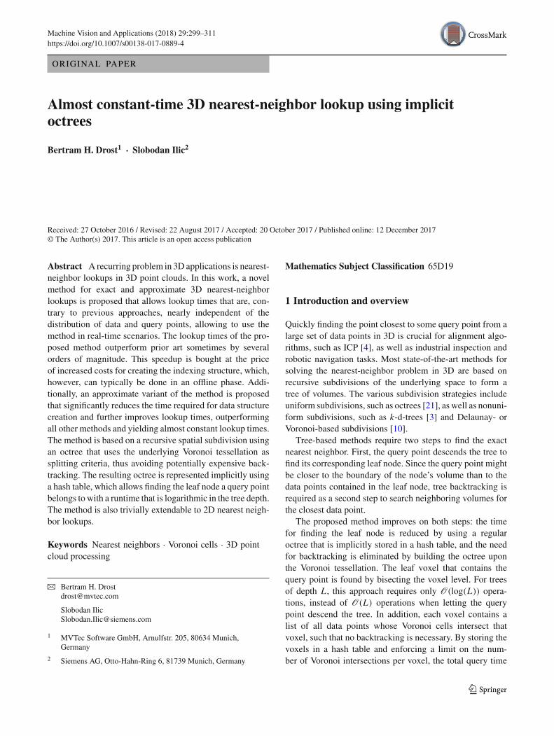
Fig. 4 Example of a degenerated point set (left) where many Voronoicells meet at one point (center). In this case, the problem of findingthe nearest neighbor is ill-posed for query points close to the center ofthe circle. To capture such degenerated cases, voxel splitting is stoppedafter Lmax subdivisions (right). See the text for more comments on whysuch situations are not of practical interest

Thus, NN(q, D) can be computed on average inO(log(log(N ))), which is almost constant.

3.5 Degenerated cases

For some degenerated cases, the proposed method for split-ting voxels based on the number of intersecting Voronoi cellsmight not terminate. This happens when more than Mmax

Voronoi cells meet at a single point, as depicted in Fig. 4.To avoid infinite recursion, a limit Lmax on the depth of theoctree is enforced. In such cases, the query time for pointsthat are within such an unsplit leaf voxel is larger than forother query points.

However, we found that in practice such cases appear onlyon synthetic datasets. Also, since the corresponding leaf vox-els are very small (of size 2−Lmax times the size of the rootvoxel), chances of a random query point to be within thecorresponding voxel are small. Additionally, note the prob-lemof finding the closest point is ill-posed in situationswheremany Voronoi cells meet at a single point and the query pointis close to that point: small changes in the query point canlead to arbitrary changes of the nearest neighbor.

The degradation in query time can be avoided by limitingthe length of L(D, v) of the corresponding leaf voxels. Themaximum error made in this case is in bound by the diameterof the voxel of level Lmax. For example, Lmax = 30 reducesthe error to 2−30 times the size of the root voxel, which isalready smaller than the accuracy of single-precision floatingpoint numbers.

Summing up, the proposed method degrades only in arti-ficial situations where the problem itself is ill-posed, but themethod’s performance guarantee can be restored at the costof an arbitrary small error.

3.6 Generalizations to higher dimensions

The proposed method theoretically can be generalized todimensions d > 3. However, memory and computational

costs would likely render the method practically unusable inhigher dimensions. This is due to several reasons:

– The branching factor 2d of the corresponding hyper-cube tree leads to exponentially increasing memory andcomputation requirements, even for approximately con-stant average tree depths. For example, even a moderatedimension such as d = 16 has a branching factor of216 = 65536, such that a tree of depth 3 would alreadyhave (216)3 = 248 nodes.

– Voronoi cells in higher dimensions are increasingly dif-ficult to compute. Dwyer [13] showed that the geometriccomplexity of the Voronoi cells of n points in dimensiond is at least1

O(ndd) (4)

– Due to the curse of dimensionality,2 the distancesbetween random points in higher dimensions tend tobecome more similar [2]. As one consequence, the num-ber of Voronoi neighbors of each point increase, up tothe point where almost all points are neighbors of eachother. As another consequence, nearest-neighbor lookupsfor a random query point become ill-conditioned in thesense that a randomquery pointwill havemanyneighborswith approximately equal distance. Voxels are thereforelikely to have very long lists of possible nearest neigh-bors, resulting in even deeper voxel trees.

4 Approximate search

4.1 Definition

Approximate nearest-neighbor methods are methods thatreturn only an approximation of the correct nearest neigh-bor. Approximate methods often are significantly faster orrequire less memory than exact methods. For example, asimple approximate method is to use a k-d-tree without per-forming backtracking (see, for example, [22,23]).

Given a query point q and a dataset D, we denoteANN(q, D) for an approximate nearest neighbor of q in D.We define the distance to the exact and the approximate near-est neighbor as

1 Note that Dwyer showed that for a fixed dimension, the complexityis linear in the number of points. Refer to equation (3.3) in [13] and thefollowing discussion for the result regarding 4.2 The term goes back to Richard E. Bellmann. It captures the fact thateven for moderately larger dimensions, the volume of space increasesdrastically. This often results in counterintuitive effects if one keepsonly 3D spaces in mind.

123

304 B. H. Drost, S. Ilic

dE = |q − NN(q, D)| (5)

dA = |q − ANN(q, D)| (6)

with dA ≥ dE.

4.2 Quality metrics

Several quantitative values can be used to describe the qualityof an approximate method. The error probability perr definesthe probability for a random query point to not return theexact, but only an approximate nearest neighbor:

perr = P(dA > dE) (7)

The absolute error is given as

Eabs = |dA − dE| = dA − dE (8)

Approximate methods are often classified according to theε-criterion, which states that

dA ≤ (1 + ε) dE (9)

and thus puts an upper bound on the relative error.Given some object M with a fixed, known size diam(M),

we will also measure the quality of an approximate nearestneighbor relative to the object’s diameter:

e = Eabs/ diam(M) = (dA − dE)/ diam(M) (10)

The proposed voxel hash method can easily be convertedinto an approximate method. We will combine two tech-niques that work at different steps of the method: List lengthlimiting and explicit voxel neighborhood.

4.3 List length limiting

A straightforward way of reducing the complexity of boththe offline and online phase is to limit the list lengths of eachvoxel. This is equivalent to storing, for each leaf node, onlya subset of the intersecting Voronoi cells. We denote LA fora subset of the correct list:

LA(D, v) ⊂ L(D, v) (11)

Several possibilities exist how LA can be selected from L .

– Minimize error probability: Given a voxel v, the probabil-ity that an intersecting Voronoi cell voro(x), x ∈ L(D, v)

contains a query point q ∈ v is

P(q ∈ voro(x) |q ∈ v) = vol(voro(x) ∩ v)

vol(v). (12)

Therefore, if x is removed from L(D, v), the probabil-ity of making an approximation error when querying forq is P(q ∈ voro(x)|q ∈ v). In order to minimize theprobability of making an error, the points in L(D, v) canbe removed based on the volume vol(voro(x) ∩ v) ofthe intersection, removing cells with smaller intersectionvolumes first. Since the Voronoi cells are disjoint, thetotal probability of an approximation error is the sum of12 over all removed entries.If the approximation error probability shall be bounded,one can remove points from the lists L(D, v) only untilsaid probability is reached.

– Minimize maximum absolute error: The Voronoi cellsintersecting a voxel canbe removed such that someprede-finedmaximum absolute error ismaintained. Given someclosed, convex, bounded volume V ⊂ R

3, we define themaximum distance of a point inside that volume from thevolume’s boundary,

maxdist(V ) = supv∈V

infw∈R3\V

|v − w| (13)

If an entry x ∈ L(D, v) is removed from L(D, v), themaximum absolute error possible is

maxdist(voro(x) ∩ v) (14)

If multiple entries x1, x2, . . . are removed, the maximumabsolute error is

max Eabs = maxdist

(⋃i

(voro(xi ) ∩ v)

)(15)

This formula allows to remove points from L(D, v)whilekeeping a bound on the maximum absolute error.

– Greedy element selection: Both methods above requirean explicit computation of the Voronoi cells and theirintersection with voxels. While elegant, such computa-tions can be expensive.A different strategy is to keep only a fixed number ofvertices that are closest to the center of the voxel. Thisstrategy is faster, since it does not require explicit compu-tation of the intersection volumes. It is especially efficientin combination with the next step, which avoids con-structing Voronoi cells all together.

4.4 Explicit voxel neighborhood

As shown in Sect. 5, using Voronoi cells as described leadsto a potentially very time-consuming offline stage. Most ofthe runtime is spent in the creation of the Voronoi cells, andthe intersection between Voronoi cells and voxels.

123

Almost constant-time 3D nearest-neighbor lookup using implicit octrees 305

Fig. 5 2D-illustration of the fast, approximate voxel creation. Insteadof computing and intersecting Voronoi cells, each point (black dot) isadded to a n × n-neighborhood (here 3 × 3) of voxels, on each voxellevel

A different approach allows a much faster assignment ofpoints to voxels: instead of intersecting Voronoi cells withvoxels, a point x ∈ D is added to the list of its neighboringvoxels only. Figure 5 illustrates this: The given point is addedto all voxels in its 3× 3 (or, in 3D, 3× 3× 3) neighborhood.

This technique is combined with the list length limitingby retaining only a few or even only one point closest to thevoxel’s center. The runtime for creating the voxel tree thisway is linear in the number of points N and has a significantlysmaller constant factor. In particular, no complex creation ofVoronoi cells needs to be performed.

Note that both steps modify only the creation of the datastructure; the lookup phase stays the same. The followingalgorithm summarizes the proposed approximate method.

Input : Dataset DVoxel level range lmin and lmaxMaximum l i s t length Mmax

for x in D do:for l from lmin to lmax do:

v ← voxel of level l containing xfor v′ in 3 × 3 × 3 neighborhood of v :L(v′) ← L(v′) ∪ {x}

for al l voxels v :Sort L(v) by distance to center of v

Truncate L(v) at length Mmax

Output : Set of voxel l i s t s L

Tree Depth For the exact methods, voxels were split basedon the number of intersecting Voronoi cells. This provideda natural way of splitting voxels only where necessary. Adownside of the proposed approximate method is that thisautomatic splitting no longer happens. As consequence, therange of levels must be specified a priori.

In the evaluation, we estimate the sampling density of thetarget point cloud D as dsampling and use it as a lower boundon the voxel size. This typically leads to tree depths of 10–30.

Additionally, a post-processing step can be used to removeunnecessary voxels: if only a single point is stored for eachvoxel (Mmax = 1), and all existing child voxels of somevoxelv store the same point, then all those child voxels can beremoved without changing the result of the nearest-neighborlookup. This effectively prunes the voxel tree at uninterestinglocations.

5 Experiments

Several experiments were conducted to evaluate the perfor-mance of the proposed method in different situations and tocompare it to the k-d-tree, the ANN library [22], the FLANNlibrary [23] and the EFANNAmethod [15] as state-of-the-artmethods. Note that the FLANN library returns an approxi-mate nearest neighbor, while ANN was configured such thatan exact nearest neighbor was returned. Both the k-d-treeand the voxel hash structure were implemented in C withsimilar optimization. The creation of the voxel data struc-ture was partly parallelized, queries were not. All times weremeasured on an Intel Xenon E5-2665 with 2.4 GHz.

5.1 Data structure creation

Although the creation of the proposed data structure is sig-nificantly more expensive than the creation of the k-d-tree,the ANN library and the FLANN library, these costs are stillwithin reasonable bounds. They are within the same orderof magnitude as for EFANNA. Figure 6, right compares thecreation times for different values of Mmax. The creation ofthe Voronoi cells is independent of the value of Mmax andthus plotted separately.

Figure 6, right shows the number of created voxels. Theydepend linearly on the number of data points,while the choiceof Mmax introduces an additional constant factor. This showsempirically what is difficult to find analytically: The octreegrowth is of the same order as a k-d-tree and requires O(N )

nodes. This leads to an average depth of the octree of depth =O(log(N )).

Note that the constant performance of the proposedmethod for fewer than 105 data points is based on our partic-ular implementation, which is optimized for large data setsand requires constant time for the creation of several caches.

5.2 Influence of implicit octree

The proposed method consists of two improvements, treebuilding based on voronoi intersection and, on top of it, theimplicit octree. To evaluate how much the implicit octree

123

306 B. H. Drost, S. Ilic

100

101

102

103

104

105

106

107

102 103 104 105 106

Num

ber

ofV

oxel

s

Number of Points

Mmax = 30Mmax = 60Mmax = 90

10−5

10−4

10−3

10−2

10−1

100

101

102

103

102 103 104 105 106

Cre

atio

nT

ime

ins

Number of Points

Mmax = 30Mmax = 60Mmax = 90

Voronoi CellsKD-Tree

ANNFLANN

EFANNA

Fig. 6 Construction and memory costs of the proposed data structurefor the CLUSTER dataset. Left: the number of created voxels dependslinearly on the size of the data cloud. As a rule of thumb, one voxel iscreated per data point. Right: the creation time of the voxel data struc-ture. The creation of the Voronoi cells is independent of the value ofMmax and its creation time is plotted separately. Although the creationof the voxel data structure is significantly slower than for the k-d-tree,theANNand the FLANN libraries, and asymptotically at the same order

of magnitude as EFANNA, the creation times are still reasonable foroffline processing. Note that the constant performance of the proposedmethod for less than 105 data points is based on our particular imple-mentation, which is optimized for large data sets and requires constanttime for the creation of several caches. Overall, larger values of Mmaxlead to faster and less memory consuming data structure creation, at theexpense of matching time (see Fig. 9)

Table 2 Speedup of the implicit, hash-based octreew.r.t. to a traditionaloctree

Dataset |D| Classic (s) Implicit (%) Speedup

ICP matching 990,998 0.34 0.25 s 26

Comparison 990,998 0.29 0.22 s 23

ICP room 260,595 0.07 0.06 s 17

helps in terms of speedup, we evaluated the Voronoi-basedoctree alone, letting query points descend the tree in a clas-sic approach. The results, shown in Table 2, show that fordatasets with around |D| ≈ 106 3D points, the runtime wasreduced by around 25%. For |D| ≈ 2.5 ∗ 105, the speedupwas 17%.

This indicates that for larger datasets, and thus deeperoctrees, the influence of the implicit octree increases. This isas expected from the theoretical analysis, since the influenceof the implicit octree (search time of O(log(depth)) insteadof O(depth)) becomes more prominent for larger depths.

5.3 Degenerated case

As discussed in Sect. 3.5, there exists degenerated caseswhere the octree creation based on Voronoi splitting wouldnot terminate. As countermeasure, we used both a maximumtree depth Lmax and a maximum list length Mmax. This wasevaluated and compared to other methods on a syntheticdataset that consists of N points distributed equally on asphere of radius 1. The query point is in the center of thesphere (Fig. 4).

As shown in Fig. 7, the non-approximate voxel-basedmethods have significant construction costs, but almost con-stant query times that are independent of the number of datapoints.

5.4 Synthetic datasets

We evaluate the performance on different datasets with dif-ferent characteristics. Three synthetic datasets were used andare illustrated in Fig. 8. For dataset RANDOM, the pointsare uniformly distributed in the unit cube [0, 1]3. For CLUS-TER, points are distributed using aGaussian distribution. ForSURFACE, points are taken from a 2Dmanifold and slightlydisturbed. For each data set, two query sets with 1,000,000points each were created. For the first set, points were dis-tributed uniformly within the bounding cube surrounding thedata point set. The corresponding times are shown in thecenter column of Fig. 9. The second query set has the samedistribution as the underlying data set, with the correspond-ing timings shown in the right column of Fig. 9.

The proposed data structure is significantly faster than thesimple k-d-tree for all datasets with more than 105 points.The ANN library shows similar performance as the proposedmethod for Mmax = 30 for the RANDOM and CLUSTERdatasets. For the SURFACE dataset, our method clearly out-performs ANN even for smaller point clouds. Note that theSURFACE dataset represents a 2D manifold and thus showsthe behavior for ICP and other surface-based applications.Overall, compared to the other methods, the performance ofthe proposed method is less dependent on the distribution of

123

Almost constant-time 3D nearest-neighbor lookup using implicit octrees 307

10−5

10−4

10−3

10−2

10−1

100

101

102

103

104

102 103 104 105 106

Cre

atio

nT

ime

ins

Number of Points

10−2

10−1

100

101

102

103

104

105

106

102 103 104 105 106

Tim

epe

rqu

ery

poin

t[µ

s]

Number of Points

Mmax = 30Mmax = 60Mmax = 90

Approximate VoxelsKD-Tree

ANNFLANN

EFANNA

Fig. 7 Construction (left) and lookup times (right) for a degenerateddataset (as shown in Fig. 4).While the voxel-basedmethods take signif-icantly longer to be created, their lookup times remains almost constant,even for larger datasets. Note that the ANN library switches to a dif-ferent internal implementation at around 102 points, leading to a dropin construction time. Also note that that the EFANNA implementation

failed to give results for less than 1000 data points, and that the voxelmethods were evaluated only up to 105 data points due to excessive con-struction times. Finally, some methods (ANN, k-d-tree, and FLANN)are linear in the number of data points. This indicates that they fall backto a brute-force search in the degenerated case, for example, due tobacktracking of the k-d-tree

RANDOM CLUSTER SURFACE

Fig. 8 Datasets used for the synthetic evaluations. The datasets showdifferent distributions of the target points in D: a uniform distributionin a unit cube (left), a Gaussian distribution forming a cluster of points

(center), and points sampled from a 2Dmanifold (right). Usually, distri-butions such as the SURFACE dataset are more relevant, since datasetstypically contain points from the surface of 3D objects

data and query points. This advantage allows our method tobe used in real-time environments.

5.5 Real-world datasets

Next, real-world examples were used for evaluating theperformance of the proposed method. Three datasets werecollected and evaluated.

ICPMatching: Several instances of an industrial object weredetected in a scene acquiredwith amulti-camera stereo setup.The original scene and the matches are shown in Fig. 10. Wefound approximate positions of the target object using themethod of [12] and subsequently used ICP for each matchfor a precise alignment. The nearest-neighbor lookups dur-ing ICP were logged and later evaluated with the availablemethods.

Comparison: We used the proposed method to find sur-face defects of the objects detected in the previous dataset.

For this, the distances of the scene points to the closestfound model were computed. The distances are visualizedin Fig. 10, right and show a systematic error in the modelingof the object.

ICP Room: Finally, we used a Kinect sensor to acquire twoslightly rotated scans of an office roomand aligned both scansusing ICP. Again, all nearest-neighbor lookups were loggedfor later evaluation.

The sizes of the corresponding data clouds and the lookuptimes are shown in Table 3. For all three datasets, the pro-posed method significantly outperforms both our k-d-treeimplementation and the ANN library by up to one order ofmagnitude.

5.6 Approximate method

We conducted several experiments to compare the proposedapproach for turning the exact voxel hash method into an

123

308 B. H. Drost, S. Ilic

Same Query DistributionRandom Query Distribution

0.01

0.1

1

10

100

102 103 104 105 106

RA

ND

OM

Tim

epe

rqu

ery

poin

t[µ

s]

Number of Points

Mmax = 30Mmax = 60Mmax = 90

KD-TreeANN

Approx. VoxelsFLANN

EFANNA

0.01

0.1

1

10

100

102 103 104 105 106

Tim

epe

rqu

ery

poin

t[µ

s]

Number of Points

0.01

0.1

1

10

100

102 103 104 105 106

CL

UST

ER

Tim

epe

rqu

ery

poin

t[µ

s]

Number of Points

0.01

0.1

1

10

100

102 103 104 105 106T

ime

per

quer

ypo

int[µ

s]

Number of Points

0.01

0.1

1

10

100

102 103 104 105 106

SUR

FAC

E

Tim

epe

rqu

ery

poin

t[µ

s]

Number of Points

0.01

0.1

1

10

100

102 103 104 105 106

Tim

epe

rqu

ery

poin

t[µ

s]

Number of Points

Fig. 9 Query time per query point for different synthetic datasets andmethods. Each row represents a different dataset. From top to bottom:RANDOM, CLUSTER, and SURFACE dataset. The x-axis shows thenumber of data points, i.e., |D|, the y-axis shows the average querytime per query point. For the center column, query points were ran-domly selected from the bounding box surrounding the data. For theright column, query points were taken from the same distribution as

the data points. Compared to other methods, the query time for theproposed method depends little on the number of data points and isalmost independent of the distribution of the data and query points. It isespecially advantageous for very large datasets as well as for datasetsrepresenting 2D manifolds. The approximate significantly outperformsall other methods for all datasets

approximate method (see Sect. 4). We varied two parametersof the approximate nearest-neighbor structure: The numberof voxels in the explicit voxel neighborhood, and the limit onthe list length, L(D, v). We allow a neighborhood radius of 1(using a 3×3×3 neighborhood of voxels on each voxel level)and 2 (5× 5× 5 neighborhood). We found that larger valueshave little benefit regarding accuracy but high computationalcosts. For the list lengths, we evaluated with limits of 1, 5 and10. We denote the approximate methods with, for example,2–5 for a voxel neighborhood of 2 and a list length limit of 5.

Table 4 compares the different exact and approximatemethods regarding data structure creation time, nearest-neighbor lookup time and approximation errors. Figure 9 alsoincludes the timings for the approximate method. In termsof nearest-neighbor lookup times, the proposed approximatemethod outperforms all other evaluated methods, sometimesby several orders of magnitude. It is the fastest method, weknow for comparable error rates, and lookup times scaleextremely well with the size of the dataset.

123

Almost constant-time 3D nearest-neighbor lookup using implicit octrees 309

Fig. 10 Example applications for the proposed method. A 3D scan ofthe scene was acquired using a multi-camera stereo setup and approxi-mate poses of the pipe joint were found using the method of [12]. Left:the poses were refined using ICP. The corresponding nearest-neighborlookups were logged and used for the evaluation shown in Table 3.

Right: for each scene point close to one of the detected objects, the dis-tance to the object is computed and visualized. This allows the detectionof defects on the surface of the objects. The lookups were again loggedand used for the performance evaluation in Table 3

Table 3 Performance in the real-world scenarios

Dataset |D| |Q| Voxel Hash, Mmax = k-d-tree (s) ANN (s) FLANN (s) EFANNA (s)

30 (s) 60 (s) 90 (s)

ICP matching 990,998 1,685,639 0.26 0.26 0.28 12.19 22.0 93.6 100.1

Comparison 990,998 2,633,591 0.22 0.25 0.30 10.62 232.1 146.3 130.3

ICP room 260,595 916,873 0.063 0.075 0.078 0.97 2.5 13.0 20.6

|D| is the number of data points, |Q| the number of query points. The proposed voxel hash structure is up to one order of magnitude faster than thecompared methods, even for large values of Mmax

Table 4 Performance of exact and approximate methods on the real-world dataset ICP Matching

Method |D| =990,998 |D| =13,333

tcreate (s) tlookup (s) Correct (%) emean emedian tcreate tlookup (s) Correct (%) emean emedian

k-d-tree 0.16 12.19 100 0 0 1.3 ms 2.1 100 0 0

ANN 0.57 23 100 0 0 17 ms 26 100 0 0

FLANN 0.37 93 12 2.4% 0.73% 6.1 ms 2 20 2.7% 0.7%

EFANNA 225 97.6 89.2 0.03% 0 9.22 s 35.2 99.8 0 0

Mmax = 30 9400 0.24 100 0 0 170 s 0.18 100 0 0

Mmax = 60 5745 0.21 100 0 0 91 s 0.14 100 0 0

Mmax = 90 5405 0.20 100 0 0 68 s 0.13 100 0 0

Approx. 1–1 14 0.13 20 1.61% 0.60% 0.2 s 0.13 23 1.61% 0.58%

Approx. 1–5 28 0.17 34 1.34% 0.35% 0.4 s 0.15 39 1.26% 0.27%

Approx. 2–1 56 0.15 37 0.54% 0.20% 0.8 s 0.14 38 0.54% 0.19%

Approx. 2–5 108 0.19 54 0.39% 0 1.3 s 0.18 61 0.35% 0

Approx. 2–10 132 0.20 60 0.35% 0 1.5 s 0.20 69 0.29% 0

Two scenarios are tested: one with a very large data cloud D of approx. one million points (left), one with a much smaller cloud of approx. tenthousand points (right). tcreate is the time required for the creation of the data structure, tlookup is the time needed to perform around 1.6 millionnearest-neighbor lookups. Correct is the ratio of points for which the returned nearest neighbor is correct and not just an approximation. Note thatthe approximate ANN library returned only correct results on this dataset. emean and emedian are the errors of the approximate nearest-neighborsearch, relative to the diameter of the target object (an error of emean = 1% would indicate that the approximate nearest neighbors have a meandistance of 1% of the object’s diameter to the exact nearest neighbor). Note that for the approximate method 1–1 with a total query time of 0.13 s,the query time per point was only 0.23 µs, around 550 CPU cycles

123

310 B. H. Drost, S. Ilic

Regarding construction times, the approximate voxelmethods are much faster than the exact voxel methods,though still significantly slower than k-d-trees, ANN,FLANN, and EFANNA.

6 Conclusion

This work proposed and evaluated a novel data structure fornearest-neighbor lookup in 3D, which can easily be extendedto 2D. Compared to traditional tree-based methods, back-tracking was made redundant by building an octree on top ofthe Voronoi diagram. In addition, a hash table was used toallow for a fast bisection search of the leaf voxel of a querypoint, which is faster than letting the query point descend thetree. The proposed method combines the best of tree-basedapproaches and fixed voxel grids. We also proposed an evenfaster approximate extension of the method.

The evaluation on synthetic datasets shows that the pro-posed method is faster than traditional k-d-trees, the ANNlibrary, the FLANN library and the EFANNA method onlarger datasets and has a query time that is almost indepen-dent of the data and query point distribution. Although theproposed structure takes significantly longer to be created,these times are still within reasonable bounds. The evalua-tion on real datasets shows that real-world scenarios, such asICP and surface defect detection, greatly benefit from the per-formance of the method. The evaluations also showed thatthe approximate variant of the method can be constructedsignificantly faster and offers unpreceded nearest-neighborquery times.

The limitations of the method are mostly in the dimensionof the data. For more than three dimensions, the construc-tion and storage costs increase more than exponentially, thusrequiring additional work tomake at least parts of themethodavailable for such data. The method is thus not suitable foronline applications, where the data must be processed imme-diately. In the future, we want to look into extensions tohigher dimensions, additional speedups of the constructionand online updates, for example, to extend datasetswith addi-tional points without completely re-computing the searchstructure.

Open Access This article is distributed under the terms of the CreativeCommons Attribution 4.0 International License (http://creativecommons.org/licenses/by/4.0/), which permits unrestricted use, distribution,and reproduction in any medium, provided you give appropriate creditto the original author(s) and the source, provide a link to the CreativeCommons license, and indicate if changes were made.

References

1. Arya, S., Mount, D.M., Netanyahu, N.S., Silverman, R., Wu, A.Y.:An optimal algorithm for approximate nearest neighbor searching

fixed dimensions. JACM 45(6), 891–923 (1998). https://doi.org/10.1145/293347.293348

2. Bellman, R.E.: Adaptive Control Processes: A Guided Tour, vol.4. Princeton University Press, Princeton (1961)

3. Bentley, J.L.: Multidimensional binary search trees used for asso-ciative searching. CACM 18(9), 509–517 (1975). https://doi.org/10.1145/361002.361007

4. Besl, P.J., McKay, N.D.: A method for registration of 3-d shapes.IEEE Trans. Pattern Anal. Mach. Intell. 14(2), 239–256 (1992).https://doi.org/10.1109/34.121791

5. Birn, M., Holtgrewe, M., Sanders, P., Singler, J.: Simple and fastnearest neighbor search. In: Blelloch, G.E., Halperin, D. (eds.)Proceedings of the Twelfth Workshop on Algorithm Engineer-ing and Experiments, ALENEX 2010, Austin, Texas, USA, 16Jan 2010, pp. 43–54. SIAM (2010). https://doi.org/10.1137/1.9781611972900.5

6. Boada, I., Coll, N., Madern, N., Sellarès, J.A.: Approximations of3d generalized voronoi diagrams. In: (Informal) Proceedings ofthe 21st European Workshop on Computational Geometry, Eind-hoven, The Netherlands, 9–11Mar 2005, pp. 163–166. TechnischeUniversiteit Eindhoven (2005)

7. Boada, I., Coll, N., Madern, N., Sellarès, J.A.: Approxima-tions of 2d and 3d generalized voronoi diagrams. Int. J. Com-put. Math. 85(7), 1003–1022 (2008). https://doi.org/10.1080/00207160701466362

8. Choi, W., Oh, S.: Fast nearest neighbor search using approximatecached k-d tree. In: 2012 IEEE/RSJ International Conference onIntelligent Robots and Systems, IROS 2012, Vilamoura, Algarve,Portugal, 7–12 Oct 2012, pp. 4524–4529. IEEE (2012). https://doi.org/10.1109/IROS.2012.6385837

9. Cleary, J.G.,Wyvill,G.:Analysis of an algorithm for fast ray tracingusing uniform space subdivision. Vis. Comput. 4(2), 65–83 (1988).https://doi.org/10.1007/BF01905559

10. Delaunay, B.: Sur la sphere vide. a la memoire de george voronoi.Bulletin de l’Académie des Sciences de l’URSS. Classe des sci-ences mathématiques et na, pp. 793–800 (1934)

11. Drost, B., Ilic, S.: A hierarchical voxel hash for fast 3d nearestneighbor lookup. In: Weickert, J., Hein, M., Schiele, B. (eds.)Pattern Recognition—35th German Conference, GCPR 2013,Saarbrücken, Germany, September 3–6, 2013. Proceedings, Lec-ture Notes in Computer Science, vol. 8142, pp. 302–312. Springer(2013). https://doi.org/10.1007/978-3-642-40602-7

12. Drost, B., Ulrich, M., Navab, N., Ilic, S.: Model globally, matchlocally: efficient and robust 3d object recognition. In: The Twenty-Third IEEE Conference on Computer Vision and Pattern Recog-nition, CVPR 2010, San Francisco, CA, USA, 13–18 June 2010,pp. 998–1005. IEEE Computer Society (2010). https://doi.org/10.1109/CVPR.2010.5540108

13. Dwyer, R.A.: Higher-dimensional voronoi diagrams in linearexpected time.DiscreteComput.Geom. 6, 343–367 (1991). https://doi.org/10.1007/BF02574694

14. Elseberg, J., Magnenat, S., Siegwart, R., Nuechter, A.: Compari-son of nearest-neighbor-search strategies and implementations forefficient shape registration. J. Softw. Eng. Robot. 3(1), 2–12 (2012)

15. Fu, C., Cai, D.: EFANNA: an extremely fast approximate nearestneighbor search algorithm based on kNN graph. ArXiv (2016).http://arxiv.org/abs/1609.07228

16. Glassner, A.S.: Space subdivision for fast ray tracing. IEEE Com-put. Graph. Appl. 4(10), 15–24 (1984)

17. Greenspan, M.A., Godin, G.: A nearest neighbor method for effi-cient ICP. In: 3rd International Conference on 3D Digital Imagingand Modeling (3DIM 2001), 28 May–1 June 2001, Quebec City,Canada, pp. 161–170. IEEE Computer Society (2001). https://doi.org/10.1109/IM.2001.924426

18. Greenspan, M.A., Yurick, M.: Approximate K-D tree search forefficient ICP. In: 4th International Conference on 3D Digital Imag-

123

Almost constant-time 3D nearest-neighbor lookup using implicit octrees 311

ing and Modeling (3DIM 2003), 6–10 Oct 2003, Banff, Canada,pp. 442–448. IEEE Computer Society (2003). https://doi.org/10.1109/IM.2003.1240280

19. Har-Peled, S.: A replacement for voronoi diagrams of near linearsize. In: 42ndAnnual SymposiumonFoundations ofComputer Sci-ence, FOCS 2001, 14–17 Oct 2001, Las Vegas, Nevada, USA, pp.94–103. IEEE Computer Society (2001). https://doi.org/10.1109/SFCS.2001.959884

20. Hwang, Y., Han, B., Ahn, H.: A fast nearest neighbor searchalgorithm by nonlinear embedding. In: 2012 IEEE Conference onComputer Vision and Pattern Recognition, Providence, RI, USA,16–21 June 2012, pp. 3053–3060. IEEE Computer Society (2012).https://doi.org/10.1109/CVPR.2012.6248036

21. Meagher, D.: Geometric modeling using octree encoding. Comput.Graph. Image Process. 19(2), 129–147 (1982). https://doi.org/10.1016/0146-664X(82)90104-6

22. Mount, D.M., Arya, S.: ANN: a library for approximate nearestneighbor searching. https://www.cs.umd.edu/~mount/ANN/

23. Muja, M., Lowe, D.G.: Fast approximate nearest neighbors withautomatic algorithm configuration. In: Ranchordas, A., Araújo,H. (eds.) VISAPP 2009—Proceedings of the Fourth InternationalConference on Computer Vision Theory and Applications, Lisboa,Portugal, 5–8Feb2009, vol. 1, pp. 331–340. INSTICCPress (2009)

24. Nüchter, A., Lingemann, K., Hertzberg, J.: Cached k-d tree searchfor ICP algorithms. In: Sixth International Conference on 3-DDigi-tal Imaging andModeling, 3DIM2007, 21–23Aug2007,Montreal,Quebec, Canada, pp. 419–426. IEEE Computer Society (2007).https://doi.org/10.1109/3DIM.2007.15

25. Samet, H.: Foundations of Multidimensional And Metric DataStructures. Morgan Kaufmann, Burlington (2006)

26. Yan, P., Bowyer, K.W.: A fast algorithm for icp-based 3d shapebiometrics. Comput. Vis. Image Underst. 107(3), 195–202 (2007).https://doi.org/10.1016/j.cviu.2006.11.001

Bertram H. Drost is a senior research engineer at MVTec SoftwareGmbH in Munich, Germany. He received a diploma in mathematicsand, in 2016, a PhD in computer science from Technische UniversitätMünchen (TUM). His current research interests include 2D and 3Dobject detection, 3D data and point cloud processing, 3D reconstructionand machine learning.

Slobodan Ilic is currently a senior key expert research scientist atSiemens Corporate Technology in Munich, Perlach. He is also a visit-ing researcher and lecturer at Computer Science Department of TUMand closely works with the CAMP Chair. From 2009 until the end of2013, hewas leading theComputerVisionGroupofCAMPatTUM, andbefore that hewas a senior researcher at Deutsche TelekomLaboratoriesin Berlin. In 2005, he obtained his PhD at EPFL in Switzerland undersupervision of Pascal Fua. His research interests include 3D recon-struction, deformable surface modelling and tracking, real-time objectdetection and tracking, human pose estimation and semantic segmen-tation.

123