Tech. Report UCL-INMA-2009.024

All roads lead to Newton: Feasible second-order methods for

equality-constrained optimization ∗

P.-A. Absil† Jochen Trumpf‡ Robert Mahony‡ Ben Andrews§

August 31, 2009

Abstract

This paper considers the connection between the intrinsic RiemannianNewton method and other more classically inspired optimization algo-rithms for equality-constrained optimization problems. We consider thefeasibly-projected sequential quadratic programming (FP-SQP) methodand show that it yields the same update step as the Riemannian Newton,subject to a minor assumption on the choice of multiplier vector. Wealso consider Newton update steps computed in various ‘natural’ localcoordinate systems on the constraint manifold and find simple condi-tions that guarantee that the update step is the Riemannian Newtonupdate. In particular, we show that this is the case for projective localcoordinates, one of the most natural choices that have been proposed inthe literature. Finally we consider the case where the full constraintsare approximated to simplify the computation of the update step. Weshow that if this approximation is good at least to second-order then theresulting update step is the Riemannian Newton update. The conclu-sion of this study is that the intrinsic Riemannian Newton algorithm isthe archetypal feasible second order update for non-degenerate equalityconstrained optimisation problems.

Key words. Feasibly-projected sequential quadratic programming (FP-SQP); equality-constrained optimization; Riemannian manifold; Riemannian Newton method; sequentialNewton method; retraction; osculating paraboloid; second-order correction; second funda-mental form; Weingarten map

∗This paper presents research results of the Belgian Network DYSCO (Dynamical Systems, Control, andOptimization), funded by the Interuniversity Attraction Poles Programme, initiated by the Belgian State,Science Policy Office. The scientific responsibility rests with its authors. This research was supported by theAustralian Research Council through the Discovery grant DP0987411.

†Departement d’ingenierie mathematique, Universite catholique de Louvain, B-1348 Louvain-la-Neuve, Bel-gium (http://www.inma.ucl.ac.be/~absil/).

‡School of Engineering, Australian National University, Australia. {firstname}.{lastname}@anu.edu.au.§Center for Mathematical Analysis, IAS, Australian National University, ACT, 0200, Australia

(Ben.Andrews@anu.edu.au).

1

1 Introduction

We consider the problem of minimizing an objective function f(x), x ∈ Rn, subject to equality

constraints Φ(x) = 0. Recall that a point x ∈ Rn is termed feasible if Φ(x) = 0, i.e., x belongs

to the feasible set M := Φ−1(0). A point that is not feasible is termed infeasible.For an arbitrary constraint function Φ, the problem of finding a feasible point close to

a present infeasible estimate, is often of similar complexity to solving the full optimisationproblem. Thus, most classical optimization methods solve the two parts of the problemconcurrently, that is, they generate a sequence of infeasible estimates that both convergeto the feasible set and to the function minimum at the same time; Sequential QuadraticProgramming (SQP) being the archetypal example of such an algorithm.

However, in a number of important examples, notably when M is a “well-behaved” sub-manifold [AMS08], the cost of forcing iterates onto the feasible set is low and maintainingfeasible iterates offers several advantages. There is no need for composite-step approachesthat attempt to reduce infeasibility while preserving a decrease of the objective function,the objective function itself can be used as a merit function, and only the structure of theobjective function on or close to the constraint set will be observed by the algorithm. More-over, in case of early termination, the algorithm returns a feasible suboptimal point, whichis often preferable to an infeasible suboptimum. Another motivation for enforcing feasibilityarises when the objective function is smooth when restricted to a certain submanifold of theoptimization domain and nonsmooth away from the manifold. This situation underlies thetheory of U-Lagrangians, and the related VU-decompositions and fast tracks [LOS00, MS00],as well as the theory of partly smooth functions [Lew02], both of which coincide in the convexcase [MM05, Th. 2.9].

Arguably the most natural approach to ensuring a feasible algorithm, at least when theconstraint condition defines a submanifold, is obtained by undertaking the optimisation inlocal coordinates directly on the feasible set. One way of obtaining local coordinates, studiedin the 1960s, is the method of direct elimination, which consists in dividing the variablesinto two groups such that the variables of the one are expressed (explicitly or implicitly)as a function of the others; see [Pol76, GL76] for an overview of the related literature. ANewton method based on direct partitioning was proposed and analyzed by Gabay and Lu-enberger [GL76]. The Riemannian Newton algorithm grew out of this work in an attempt tofind a unifying framework for computation of the update step [Gab82, Shu86, Udr94, Smi94].In the 1990s, the nature of the constraint sets were considered in more detail and a number ofimportant examples with significant Lie group and homogeneous space structures were iden-tified [HM94], and the explicit form of the Newton algorithm for several examples such as theGrassmann manifold were computed [EAS98]. More recent work [ADM+02, HT04, AMS08]has developed a coherent theory of intrinsic Newton methods on structured manifolds witha particular emphasis on practical issues of implementation. The approach has led to anumber of highly competitive algorithms for problems where the constraint set has suitablestructure, e.g., algorithms for the extreme eigenvalue problem [ABG06, BAG08], rank reduc-tion of correlation matrices [GP07], semidefinite programming [JBAS08], and stereo visionprocessing [HHLM07].

Another recent development concerning feasible second-order methods proceeds from theSQP approach. The classical SQP is not a feasible method: even if Φ(xk) = 0, it is likely thatΦ(xk+1) 6= 0; see, e.g., [NW06, Ch. 18]. However, in recent work, Wright and Tenny [WT04]proposed a feasibly-projected SQP (FP-SQP) method, that generates a sequence of feasible it-

2

erates by solving a trust-region SQP subproblem at each iteration and perturbing the resultingstep to retain feasibility. “By retaining feasibility, the algorithm avoids several complicationsof other trust-region SQP approaches: the objective function can be used as a merit function,and the SQP subproblems are feasible for all choices of the trust-region radius” [WT04]. Thiscan be highly advantageous in situations where the computational cost of ensuring feasibilityis negligible compared to the overall cost of the optimization algorithm.

Finally, we mention that the concepts of U-Lagrangian and partly smooth functions ledto several Newton-like algorithms whose iterates are constrained to a submanifold M suchthat the restriction f|M is smooth. These algorithms are unified in [DHM06] under a commontwo-step, predictor-corrector form, and connections with SQP and Riemannian Newton arestudied in [MM05].

In this paper, we investigate the similarities between feasible second-order optimisationalgorithms that follow from an extrinsic viewpoint, that is an algorithm posed on the overar-ching space R

n with additional constraints embedded in this space, SQP being the archetypalexample, as compared to algorithms that follow from an intrinsic viewpoint, that is algorithmsposed explicitly on the constraint set, the Riemannian Newton being the archetypal example.The reason for the title, “All roads lead to Newton”, is that this paper extends and rein-forces the message, already implicitly present in the taxonomy constructed in [EAS98], thatall feasible second-order methods for equality-constrained optimization are an intrinsic New-ton algorithm, or at the very least, only vary from the Newton algorithm in non-substantiveaspects.1 It is important to note that our conclusions only hold on the intersection of theproblem spaces for the different approaches, that is, where an intrinsic Newton is derivedfor an embedded submanifold (such algorithms can be applied to a wider class of problems[AMS08]) and where an extrinsic-viewpoint algorithm is constrained to have feasible iteratesat every step.

In detail, we consider the Feasibly-Projected Sequential Quadratic Program (FP-SQP)[WT04] and show that (for a least-squares choice of the Lagrange multiplier λk and ignoringthe trust region and other modifications) the algorithm is “intrinsic” to the feasible set andcan be interpreted as a Riemannian Newton method. We also consider the intrinsic algorithmobtained by applying the Newton method in local coordinates on M. We show that if the localcoordinates chosen have a simple second-order rigidity condition at the iterate point then onerecovers the Riemannian Newton as expected. A simple proof that the most natural choiceof local coordinates, the projective coordinates (those coordinates obtained by projectingthe tangent plane of a submanifold back onto the submanifold) satisfy the required rigidityconditions is provided. It is well known that the Newton method only uses second-orderinformation from the cost. We demonstrate that it also uses second order information onthe constraint set. This leads to a discussion of alternatives where the constraint set Mis replaced by an approximation Mxk

at each iteration. We propose ways of constructing

approximations Mx that admit a simple expression and that agree to second order with M

1In fact, the proverb “all roads lead to Rome” was never itself a Roman proverb and the earliest referencewe know of is [dL75] “mille viae ducunt homines per saecula Romam” or “a thousand roads lead men foreverto Rome”. In his discourse on the Astrolab [Cha91] Chaucer states “diverse pathes leden diverse folk therighte way to Rome,” and the saying was popularised by Jean de La Fontaine (“Le Juge arbitre, l’Hospitalier,et le Solitaire”, Fables, livre XII) “Tous chemins vont a Rome; ainsi nos concurrents crurent pouvoir choisirdes sentiers differents.” The historic versions of the quote are as well adapted to our message as the modernversion; using our analogy they say roughly, however you derive a second-order feasible method for an equalityconstrained optimisation problem, and even if you believe you are doing something novel, you will still end upwith an algorithm that is in essence an intrinsic Newton update.

3

at x.The reader familiar with [MM05] will find an important overlap between the two works.

This paper, however, departs from [MM05] in several ways. The convexity assumption isdropped. The Riemannian Newton method is considered in the general retraction-basedsetting of [ADM+02, §5], instead of being limited to the three tangential, exponential, andprojection parameterizations. Proposition 4.2 shows that Sequential Newton [MM05, Alg. 1.8]yields the same Newton vector for all second-order retractions. The link between RiemannianNewton and SQP is extended to the feasibly-projected SQP of [WT04] and concerns thewhole iteration rather than just the Newton vector. Equation 3.6 in [MM05] is used to obtainexpression (34) showing that M enters the Riemannian Hessian through its tangent spaceand the second derivative of its tangential parameterization only. The extrinsic expression ofthe Riemannian Hessian in [MM05, Th. 3.4] is rewritten in (41) in terms of the derivative ofthe projector, which leads to rich interpretations in terms of the curvature of the manifold(see Section 6.1).

Even though some methods discussed in this paper stem from differential-geometric con-cepts, we do not assume any background in differential geometry beyond a basic knowledgein real analysis in the main body of the paper. In particular, the formulation of the methodssolely relies on matrix computation and calculus. For completeness, we also provide a finalsection to the paper that provides the full geometric picture in the modern language of dif-ferential geometry. In particular, we show that the intrinsic Newton algorithm depends on,and only on, a second order approximation of the cost and the Riemannian curvature of theconstraint set in its update.

Section 2 introduces notation and assumptions, Section 3 deals with SQP, Section 4 withintrinsically-built Newton methods, and Section 5 with approximations of M. Section 6studies the role of the curvature of M in the Riemannian Hessian, and the paper ends withconcluding remarks.

2 Problem definition, concepts, and notation

In this section, we present the optimization problem considered and we explain in plaincalculus language how it relates to optimization on manifolds.

We consider the general equality-constrained optimization problem

min f(x) subject to Φ(x) = 0, (1)

where the objective function f : Rn → R and the constraint function Φ : R

n → Rm are C2.

The Euclidean gradient of f at x will be denoted by ∇f(x) =[∂1f(x) . . . ∂nf(x)

]Tand

its Hessian matrix by ∇2f(x). For a differentiable matrix-valued function F , we let DF (x)[z]denote the directional derivative of F at x along z. If F is vector valued, then DF (x) alsodenotes the Jacobian matrix of F at x and DF (x)z stands for DF (x)[z]. We also find itconvenient to use the notation ∇Φ(x) = DΦ(x)T =

[∇Φ1(x) . . . ∇Φm(x)

].

For the purpose of relating SQP to Newton on manifolds, we assume that the linear in-dependence constraint qualification (LICQ) holds at all points of Φ−1(0), that is the columnsof ∇Φ(x) are linearly independent for all x ∈ Φ−1(0); see, e.g., [BGLS03, §11.3]. The value0 is then said to be a regular value of Φ, and a well-known theorem in differential geome-try [AMR88, §3.5.3] ensures that

M := Φ−1(0) = {x ∈ Rn : Φ(x) = 0}

4

is a d-dimensional submanifold (also called embedded submanifold) of Rn, where

d = n − m.

This means that the subset M of Rn is locally a d-slice, that is, around every point x ∈ M,

there is an open set U in Rn and a coordinate system on U such that M∩ U corresponds to

the points where all but the d first coordinates vanish [AMR88, §3.2.1]. The tangent spaceto M at a point x is ker(∇Φ(x)T ) and is denoted by TxM. Observe that TxM is a linearsubspace of R

n, hence its elements are naturally identified with elements of Rn. We let

Px = I −∇Φ(x)(∇Φ(x)T∇Φ(x))−1∇Φ(x)T (2)

denote the orthogonal projector onto TxM. Observe that P is a smooth matrix-valued func-tion. Note also that the expression (2) still makes sense when x is not in M, provided thatthe columns of ∇Φ(x) are linearly independent.

The manifold M is naturally a Riemannian submanifold of Rn. This means that the

tangent spaces to M are naturally equipped with an inner product that varies smoothly withthe base point of the tangent space:

〈z1, z2〉x = zT1 z2, z1, z2 ∈ TxM. (3)

Since M is a Riemannian submanifold, there is a well-defined notion of gradient and Hessianof f in the sense of M, which we denote by grad f|M(x) and Hess f|M(x); see Section 4.1or [AMS08] for details.

An iterative optimization method A on M takes an objective function f to an iterationmap Af : M → M. Given an objective function f and an initial point x0 ∈ M, the purposeof the method is to create a sequence on M defined by xk+1 := Af (xk). We say that the

iterative optimization method A is intrinsic to M if f|M = f|M implies that Af = Af. In

other words, the iteration map Af does not change if f is modified outside M. As we willsee, an intrinsic method may have extrinsic implementations, i.e., implementations that usesubroutines that are not intrinsic. Note also that if we are only given f|M, we can still useextrinsic implementations of intrinsic methods, provided that we have a routine that takesf|M as input and extends it outside M. How we extend it, apart from guaranteeing suitablesmoothness, does not matter for an intrinsic method. Several of the algorithms studied inthis paper have this property.

3 Sequential Quadratic Programming

Sequential Quadratic Programming (SQP) for problem (1) can be introduced as follows (see,e.g., [NW06, BGLS03]). The KKT necessary conditions for optimality are

{∇f(x) + ∇Φ(x)λ = 0

Φ(x) = 0,(4)

λ ∈ Rm. Points x∗ for which there exists λ∗ such that (4) is satisfied are termed stationary

points. Linearizing the KKT system (4) at (x, λ) and denoting by (z, λ+ − λ) the variation

5

of the variables x and λ respectively, we obtain the system(∇2f(x) +

m∑

i=1

∇2Φi(x)λi

)z + ∇f(x) + ∇Φ(x)λ+ = 0 (5a)

∇Φ(x)T z + Φ(x) = 0. (5b)

Following [AT07], we refer to (5) as the Newton-KKT equations. The pure Newton step forsolving (4) is given by (x, λ) 7→ (x+, λ+) = (x + z, λ+), where z and λ+ solve (5).

The name SQP for methods based on (5) stem from the fact that the Newton-KKTequations can be viewed as the KKT equations of the quadratic problem (QP)

minz

zT∇f(x) + 12zT (∇2f(x) +

m∑

i=1

∇2Φi(x)λi)z

subject to ∇Φ(x)T z + Φ(x) = 0,

In preparation for the comparison with Newton’s method on M, observe that, when x isfeasible (i.e., x ∈ M), the Newton-KKT equations (5) are equivalent to

Px(∇2f(x) +m∑

i=1

∇2Φi(x)λi)z = −Px∇f(x) (6a)

∇Φ(x)T z = 0 (6b)

∇Φ(x)T (∇2f(x) +m∑

i=1

λi∇2Φi(x))z + ∇Φ(x)T∇Φ(x)λ+ = 0 (6c)

where Px denotes the orthogonal projector (2), and where we have used the identity Px∇Φ(x) =0. Equation (6) can be solved by obtaining z from (6a)-(6b) and then solving (6c) for λ+.

Observe also that, given x ∈ M, the LICQ condition ensures that the first equation in (4)has a unique least-squares solution

λ(x) = −(∇Φ(x)T∇Φ(x))−1∇Φ(x)T∇f(x). (7)

3.1 FP-SQP

Most variants of SQP found in the literature are infeasible, i.e., the condition that the iteratesxk belong to M is not enforced. An exception is the feasibly-projected sequential quadraticprogramming (FP-SQP) algorithm of Wright and Tenny [WT04]. In that algorithm, a firststep z is obtained by solving a problem of the form (5) at a feasible point x ∈ M, undera trust-region constraint. Then, a perturbation z of the step z is found with the followingproperties: feasibility, i.e.,

x + z ∈ M, (8)

and asymptotic exactness, that is, there is a continuous monotonically increasing functionφ : R

+ → R+ with φ(0) = 0 such that

‖z − z‖ ≤ φ(‖z‖2)‖z‖2. (9)

(In [WT04], φ is required to be into [0, 1/2], for the purpose of obtaining a global convergenceresult under the trust-region constraint. This restriction is not needed in the context of the

6

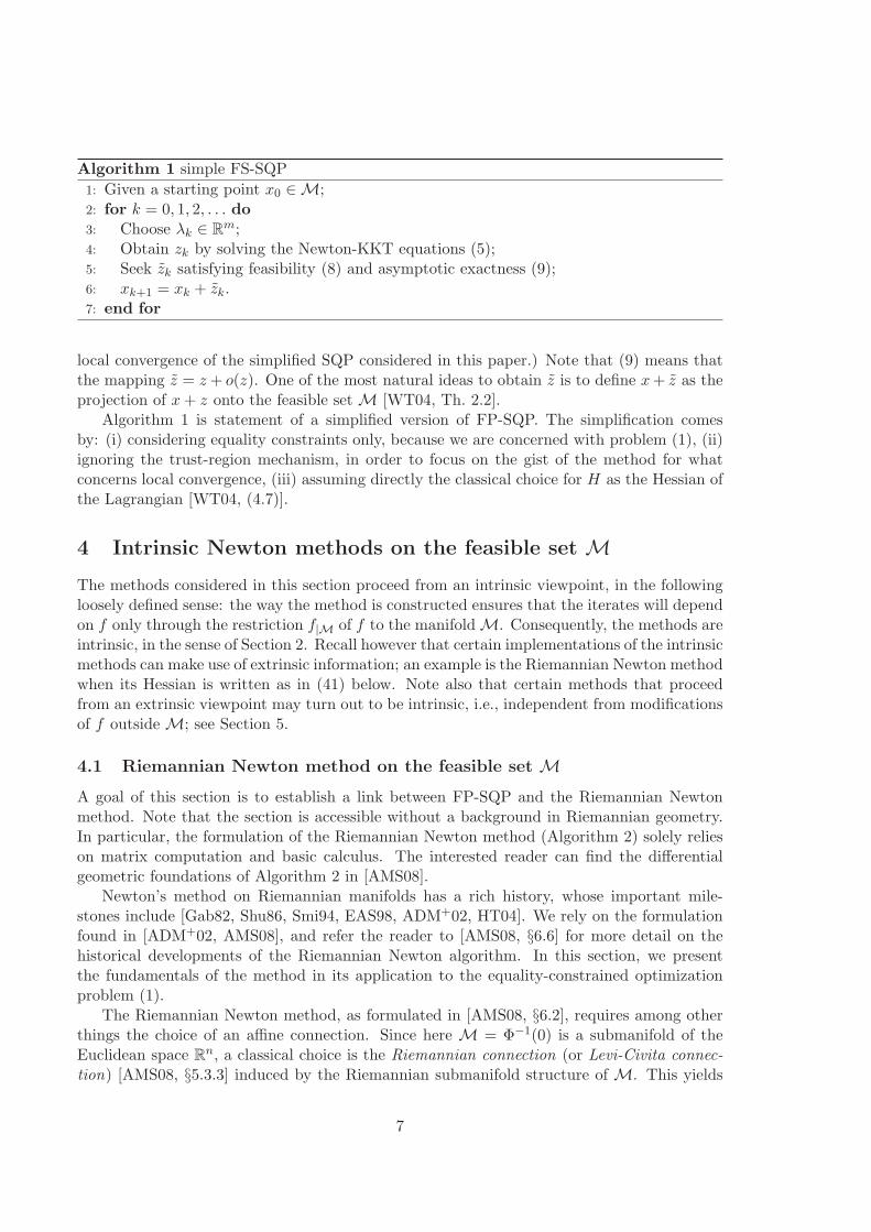
Algorithm 1 simple FS-SQP

1: Given a starting point x0 ∈ M;2: for k = 0, 1, 2, . . . do3: Choose λk ∈ R

m;4: Obtain zk by solving the Newton-KKT equations (5);5: Seek zk satisfying feasibility (8) and asymptotic exactness (9);6: xk+1 = xk + zk.7: end for

local convergence of the simplified SQP considered in this paper.) Note that (9) means thatthe mapping z = z + o(z). One of the most natural ideas to obtain z is to define x + z as theprojection of x + z onto the feasible set M [WT04, Th. 2.2].

Algorithm 1 is statement of a simplified version of FP-SQP. The simplification comesby: (i) considering equality constraints only, because we are concerned with problem (1), (ii)ignoring the trust-region mechanism, in order to focus on the gist of the method for whatconcerns local convergence, (iii) assuming directly the classical choice for H as the Hessian ofthe Lagrangian [WT04, (4.7)].

4 Intrinsic Newton methods on the feasible set M

The methods considered in this section proceed from an intrinsic viewpoint, in the followingloosely defined sense: the way the method is constructed ensures that the iterates will dependon f only through the restriction f|M of f to the manifold M. Consequently, the methods areintrinsic, in the sense of Section 2. Recall however that certain implementations of the intrinsicmethods can make use of extrinsic information; an example is the Riemannian Newton methodwhen its Hessian is written as in (41) below. Note also that certain methods that proceedfrom an extrinsic viewpoint may turn out to be intrinsic, i.e., independent from modificationsof f outside M; see Section 5.

4.1 Riemannian Newton method on the feasible set M

A goal of this section is to establish a link between FP-SQP and the Riemannian Newtonmethod. Note that the section is accessible without a background in Riemannian geometry.In particular, the formulation of the Riemannian Newton method (Algorithm 2) solely relieson matrix computation and basic calculus. The interested reader can find the differentialgeometric foundations of Algorithm 2 in [AMS08].

Newton’s method on Riemannian manifolds has a rich history, whose important mile-stones include [Gab82, Shu86, Smi94, EAS98, ADM+02, HT04]. We rely on the formulationfound in [ADM+02, AMS08], and refer the reader to [AMS08, §6.6] for more detail on thehistorical developments of the Riemannian Newton algorithm. In this section, we presentthe fundamentals of the method in its application to the equality-constrained optimizationproblem (1).

The Riemannian Newton method, as formulated in [AMS08, §6.2], requires among otherthings the choice of an affine connection. Since here M = Φ−1(0) is a submanifold of theEuclidean space R

n, a classical choice is the Riemannian connection (or Levi-Civita connec-tion) [AMS08, §5.3.3] induced by the Riemannian submanifold structure of M. This yields

7

Algorithm 2, for which some explanations are in order.

Algorithm 2 Riemannian Newton method on Φ−1(0)

1: Given a retraction R on Φ−1(0) and a starting point x0 ∈ Φ−1(0);2: for k = 0, 1, 2, . . . do3: Solve, for the unknown zk ∈ ker(DΦ(xk)), the Newton equation

PxkD(P∇f)(xk)[zk] = −Pxk

∇f(xk), (10)

where Px denotes the orthogonal projector (2) onto ker(DΦ(x)).4: Set

xk+1 := Rxk(zk).

5: end for

LetTM =

⋃

x∈M

(x, TxM) (11)

denote the tangent bundle of M. A retraction R [ADM+02] (or see [AMS08, §4.1] for thepresent equivalent formulation) is a smooth mapping from a neighborhood of M in TM,taking its values in M, and satisfying the following properties: Let Rx denote the restrictionof R to (x, TxM) ≃ TxM, then

Rx(0x) = x, (12a)

where 0x denotes the origin of the vector space TxM, and

d

dtRx(tξx)

∣∣∣∣t=0

= ξx, for all ξx ∈ TxM. (12b)

The notationD(P∇f)(xk)[zk]

in (10) stands for the derivative at xk along zk of the function that maps x to Px∇f(x).Because Px∇f(x) is the gradient of f at x in the sense of the Riemannian submanifoldM [AMS08, (3.37)], we adopt the notation

grad f|M(x) := Px∇f(x). (13)

For similar reasons [AMS08, (5.15)], we have

Hess f|M(x) := PxD(grad f|M

)(x) (14)

= PxD(P∇f)(x).

The Riemannian Newton method (Algorithm 2) can thus be compactly written as the iterationx 7→ x+ computed as

Hess f|M(x)z = −grad f|M(x), z ∈ TxM (15a)

x+ = Rx(z). (15b)

Observe that the only freedom in Algorithm 2 is in the choice of the retraction R. In orderto relate this algorithm with FP-SQP, we need to develop Newton’s equation (15a), i.e., (10).We first do it for the case where M is a hypersurface, then for the general case.

8

4.1.1 Newton’s method on hypersurfaces

We first consider the case m = 1, i.e., the constraint function Φ is a real-valued function andthus the manifold M = Φ−1(0) has codimension 1. Let x ∈ M, i.e., Φ(x) = 0. Let λ be theleast-squares multipliers (7), i.e.,

λ(x) = −(∇Φ(x)T∇Φ(x))−1∇Φ(x)T∇f(x) ∈ R. (16)

Then, from (13) and the expression of Px (2),

grad f|M(x) = Px∇f(x) = ∇f(x) + λ(x)∇Φ(x)

and, for all z ∈ TxM, the Riemannian Hessian Hess f|M satisfies

Hess f|M(x)z = PxDgrad f|M(x)z = Px(∇2f(x) + λ(x)∇2Φ(x))z, (17)

where we have used Px∇Φ(x) = 0. Newton’s equation (15a) thus reads

Px(∇2f(x) + λ(x)∇2Φ(x))z = −Px∇f(x), ∇Φ(x)T z = 0. (18)

This equation corresponds to FP-SQP’s (6a)-(6b) in the particular case where λ is chosenaccording to (16).

4.1.2 General case

We now consider the general case m ≥ 1, i.e., the constraint function Φ is in general avector-valued function. Let x ∈ M, i.e., Φ(x) = 0. Let λ be as in (7), that is,

λ(x) = −(∇Φ(x)T∇Φ(x))−1∇Φ(x)T∇f(x) ∈ Rm. (19)

We have, from (13) and the expression of Px (2),

grad f|M(x) = Px∇f(x) = ∇f(x) + ∇Φ(x)λ(x)

and, for all z ∈ TxM, the Riemannian Hessian Hess f|M satisfies

Hess f|M(x)z = PxD(grad f|M)(x)[z]

= Px∇2f(x)z + PxD∇Φ(x)[z]λ(x) (20)

= Px∇2f(x)z − PxD∇Φ(x)[z](∇Φ(x)T∇Φ(x))−1∇Φ(x)T∇f(x), (21)

where we have used the identity Px∇Φ(x) = 0. Newton’s equation (15a) becomes

Px∇2f(x)z + PxD∇Φ(x)[z]λ(x) = −Px∇f(x), ∇Φ(x)T z = 0. (22)

Observe that this equation is again FP-SQP’s (6a)-(6b) for the special choice (7) of λ.The next result formalizes the relation between FP-SQP and the Riemannian Newton

method.

Proposition 4.1 (Riemannian Newton and FP-SQP) Assume as always that 0 is aregular value of Φ, so that the set M is an embedded submanifold of R

n. Then simple FP-SQP(Algorithm 1), with λ in Step 3 chosen as in (7) and with z in Step 5 chosen as a smoothfunction of (x, z), is the Riemannian Newton method (Algorithm 2) with the retraction definedby R : z 7→ x + z. Vice-versa, Algorithm 2 is Algorithm 1 with z := R(z) − x.

Proof. For the first claim, it remains to show that that R : z 7→ x + z is a retraction. Thisdirectly follows from the smoothness assumption on z and from (8)-(9). For the second claim,in view of (12), it is clear that z := R(z) − x satisfies (8)-(9). �

9

4.1.3 Remarks

Let L(x, λ) = f(x) + Φ(x)λ, and observe that the left-hand side of (6a) is Px∇2L(·, λ)(x)z.

In the case where λ is chosen as in (7), the link

Px∇2L(·, λ(x))(x)z = Hess f|M(x)[z], z ∈ TxM

between the Hessian of the Lagrangian and the Riemannian Hessian has been known since [EAS98,§4.9], and the relation at the critical points of f|M can already be found in Gabay [Gab82].Here, by relying on the retraction-based Newton method, we have shown that the overallalgorithms overlap. A consequence is that the convergence analysis of the one can benefit theother.

Note that, even though they coincide under the above assumptions, FP-SQP and Newtonon manifolds are not identical methods. FP-SQP makes no assumption on λk beyond thefact that it must converge to the correct value, whereas Newton on manifolds requires λk tobe defined by (7). On the other hand, the intrinsic Newton algorithm on manifolds is notrestricted to manifolds that come to us in the form M = {x ∈ R

n : Φ(x) = 0}; see, e.g.,quotient manifolds [AMS08]. Indeed, some of the more abstract manifolds provide the mostsuccessful intrinsic Newton algorithms developed to date [EAS98, ADM+02, HT04].

We opted for the Levi-Civita connection on M, hence the projector Px in the definitionof the Hessian (14) is the orthogonal projector onto the tangent space. However, the analysisof Newton’s method on manifolds in [ADM+02, AMS08] does not require any assumption onthe choice of the affine connection. Choosing a non-orthogonal projector in (14) amounts tochoosing a different affine connection to the Riemannian Levi-Civita connection, which leadsto a different update step, However, the algorithm is still an intrinsic Newton algorithm, andthe full convergence theory will still apply [AMS08].

There is a similar link between the trust-region FP-SQP [WT04] and the Riemanniantrust-region method proposed in [ABG07].

4.2 Newton’s method in coordinates: Sequential Newton

A natural approach to obtain an intrinsic second-order method is to perform a Newton methodon the objective function expressed in local coordinates of M. In this section, we show thatfor certain choices of the retraction R, the Riemannian Newton step (Algorithm 2) at anyx ∈ M—and thus the simple FP-SQP (Algorithm 1) under the conditions of Proposition 4.1—can be interpreted as a “classical” Newton step on the inner product space TxM for theobjective function f ◦ Rx. (The inner product on TxM comes naturally by viewing it as alinear subspace of R

n.)Newton’s method in coordinates is defined in Algorithm 3, where ∇(f ◦ Rx) denotes the

gradient of f ◦ Rx and ∇2(f ◦ Rx) denotes its Hessian. They are well defined, since TxM isa linear subspace of R

n and thus inherits an inner product. The name Sequential Newton isborrowed from [MM05, Alg. 1.8]; see remark in Section 4.2.2.

A sufficient condition for (23) to be equivalent to the Riemannian Newton method (Al-gorithm 2) with retraction R is that R be a second-order retraction, which means that, inaddition to the properties (12), we have

Pxd2

dt2Rx(tξx)

∣∣∣∣t=0

= 0. (24)

10

Algorithm 3 Sequential Newton

1: Given a retraction R on Φ−1(0) and a starting point x0 ∈ Φ−1(0);2: for k = 0, 1, 2, . . . do3: Solve, for the unknown zk ∈ ker(DΦ(xk)), the Newton equation

∇2(f ◦ Rx)(0x)zk = −∇(f ◦ Rx)(0x). (23a)

4: Setxk+1 = Rxk

(zk). (23b)

5: end for

Indeed, because R is a retraction, we can appeal to [AMS08, (4.4)] to conclude that

∇(f ◦ Rx)(0x) = grad f|M(x), (25)

and when R is second-order, we can also appeal to [AMS08, Pr. 5.5.5] to conclude that

∇2(f ◦ Rx)(0x) = Hess f|M(x). (26)

where Hess f|M is as in (14). From (25) and (26), it follows that (23) reduces to the Rieman-nian Newton method (15).

While (25) is direct, (26) requires more work. For the reader’s convenience, we specializethe general proof [AMS08, Pr. 5.5.5] to the present case.

Proposition 4.2 (Riemannian Newton and Sequential Newton) If R is a second-orderretraction, then (26) holds, with Hess f|M(x) as in (14). Consequently, given a second-orderretraction R, Riemannian Newton (Algorithm 2) and Sequential Newton (Algorithm 3) areequivalent.

Proof. Since the two sides of (26) are Hessians, thus symmetric operators, it is sufficient (inview of the polarization identity) to show that, for all z ∈ TxM, we have zT∇2(f ◦Rx)(0x)z =zT Hess f|M(x)[z]. We develop the left-hand side:

zT∇2(f ◦ Rx)(0x)z =d2

dt2f ◦ Rx(tz)

∣∣∣∣t=0

=d

dt

(d

dtf ◦ Rx(tz)

)∣∣∣∣t=0

=d

dt

(∇f(Rx(tz))T d

dtRx(tz)

)∣∣∣∣t=0

=d

dt

(∇f(Rx(tz))TPRx(tz)

d

dtRx(tz)

)∣∣∣∣t=0

11

since ddt

Rx(tz) ∈ TRx(tz)M

=d

dt

(PRx(tz)∇f(Rx(tz))

)T∣∣∣∣t=0

d

dtRx(z)

∣∣∣∣t=0

+ ∇f(x)TPxd2

dt2Rx(tz)

∣∣∣∣t=0

=d

dt

(PRx(tz)∇f(Rx(tz))

)T∣∣∣∣t=0

z

since ddt

Rx(z)∣∣t=0

= z and Pxd2

dt2Rx(tz)

∣∣∣t=0

= 0

=

(D(P∇f)(Rx(0x))

d

dtRx(tz)

∣∣∣∣t=0

)T

z

= zT D(P∇f)(x)z

= zT Hess f|M(x)[z].

�

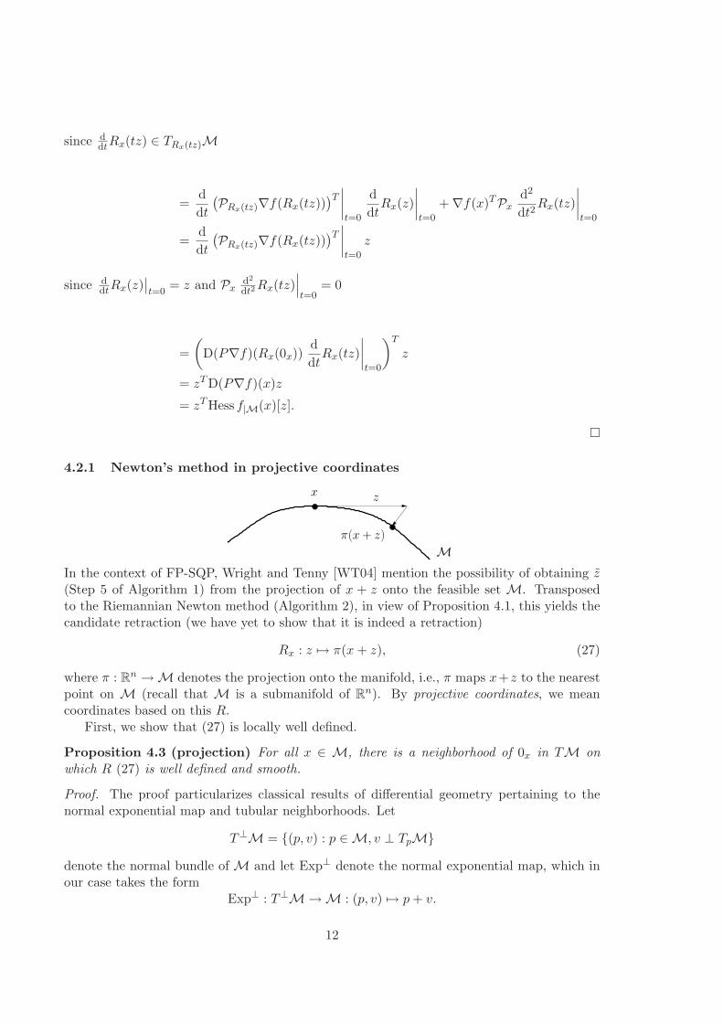
4.2.1 Newton’s method in projective coordinates

M

x

π(x + z)

z

In the context of FP-SQP, Wright and Tenny [WT04] mention the possibility of obtaining z(Step 5 of Algorithm 1) from the projection of x + z onto the feasible set M. Transposedto the Riemannian Newton method (Algorithm 2), in view of Proposition 4.1, this yields thecandidate retraction (we have yet to show that it is indeed a retraction)

Rx : z 7→ π(x + z), (27)

where π : Rn → M denotes the projection onto the manifold, i.e., π maps x+z to the nearest

point on M (recall that M is a submanifold of Rn). By projective coordinates, we mean

coordinates based on this R.First, we show that (27) is locally well defined.

Proposition 4.3 (projection) For all x ∈ M, there is a neighborhood of 0x in TM onwhich R (27) is well defined and smooth.

Proof. The proof particularizes classical results of differential geometry pertaining to thenormal exponential map and tubular neighborhoods. Let

T⊥M = {(p, v) : p ∈ M, v ⊥ TpM}

denote the normal bundle of M and let Exp⊥ denote the normal exponential map, which inour case takes the form

Exp⊥ : T⊥M → M : (p, v) 7→ p + v.

12

It is known [Sak96, II.4.3] that for all x ∈ M, Exp⊥ is a diffeomorphism (and thus a one-to-one map) on a neighborhood U of 0x in T ⊥ M onto the neighborhood Exp⊥(U) of x. Chooseǫ > 0 smaller than half of the radius of a (nonempty) ball around x contained in Exp⊥(U).Then, for all q ∈ Bǫ, π(q) belongs to M∩ Exp⊥(U) and by a standard optimality argumentmust satisfy Exp⊥(vπ(q)) = q for some vπ(q) ∈ T⊥

π(q)M. Since Exp⊥ is a diffeomorphism on U ,

it follows that π(q) = pj1(Exp⊥)−1(q), where pj1((p, v)) := p. Hence π(p + z) is well definedand smooth for all p ∈ M and all z ∈ TpM with ‖p − q‖ < ǫ/2 and ‖z‖ < ǫ/2. �

Proposition 4.4 (projective retraction) The R mapping (27) is a retraction. Moreover,it is a second-order retraction.

Proof. Let x ∈ M, z ∈ TxM, and consider the curve γ : t 7→ π(x + tz). We need to showthat γ′(0) = z (hence R is a retraction) and that γ′′(0) ∈ (TxM)⊥ (hence R is a second-orderretraction). We have

γ(t) = x + tz − ‖x + tz − γ(t)‖︸ ︷︷ ︸:=µ(t)

Nγ(t),

where Nγ(t) belongs to (Tγ(t)M)⊥. Thus

γ′(t) = z − µ′(t)Nγ(t) − µ(t)N ′γ(t),

andγ′′(t) = −µ′′(t)Nγ(t) − µ′(t)N ′

γ(t) − µ′(t)N ′γ(t) − µ(t)N ′′

γ(t).

Observe that µ(0) = 0, and since

µ′(t) =1

µ(t)〈z − γ′(t), x + tz − γ(t)〉 = 〈z, Nγ(t)〉,

we have µ′(0) = 〈z, Nx〉 = 0. Hence

γ′(0) = z and γ′′(0) = −µ′′(t)Nx ∈ (TxM)⊥.

�

Proposition 4.5 (projective Newton) Newton’s method in projective coordinates (Algo-rithm 3 with R as in (27)) is equivalent to the Riemannian Newton method (Algorithm 2)with R as in (27).

Proof. Direct from Propositions 4.2 and 4.4. �

4.2.2 Remarks

Algorithm 3 is identical to [MM05, Alg. 1.8], except that the first-order condition (12b) isnot enforced in the latter. Nevertheless, Algorithm 3 is not more restrictive than [MM05,Alg. 1.8]. Indeed, if ϕx satisfies the properties of a retraction except for (12b), then Rx :=ϕx ◦ (Dϕx(0))−1 is a retraction, and we have that the mapping x 7→ x+ defined by

∇2(f ◦ ϕx)(0x)z = −∇(f ◦ ϕx)(0x) (28a)

x+ = ϕx(z) (28b)

13

is the same as (23). To see this, observe that

∇2(f ◦ Rx)(0x)z = Dϕx(0x)−T∇2(f ◦ ϕx)(0x)Dϕx(0x)−1z

for all z ∈ TxM, and

∇(f ◦ Rx)(0x) = Dϕx(0)−T∇(f ◦ ϕx)(0x).

Note that the domain of the parameterizations ϕx is (a subset of) the tangent spaceTxM, and not (a subset of) R

d. Strictly speaking, they are thus not parameterizations in thesense of differential geometry (see, e.g., [dC92]), because identifying TxM with R

d requiresto choose a basis of TxM. In [HT04], parameterizations are defined on open subsets of R

d.Both approaches have advantages and drawbacks; see in particular the discussion in [AMS08,§4.1.3].

Several examples of second-order retractions can be found in [AM09].The fact that the Riemannian Newton method converges quadratically does not follow

straightforwardly from Proposition 4.5, because the objective function f ◦Rx and its domainTxM change at each step as x changes. Showing quadratic convergence requires some work,which can be found in [HT04, AMS08].

5 Methods based on approximations of M

In this section, we tackle the general equality-constrained optimization problem (1) by con-sidering at the current iterate x the subproblem

min f(x) subject to x ∈ Mx, (29)

where the submanifold Mx is some approximation of class C2 of the submanifold M = Φ−1(0).

This is thus an extrinsic approach: evaluating f on M means in general evaluating f outsideM. We give conditions on Mx, termed second-order agreement (defined next), such that theNewton vector at x for (29) and the one for the original problem (1) coincide.

We require that Mx contains x and that the tangent spaces match, i.e., TxMx = TxMthought of as subspaces in R

n. To define the notion of second-order agreement at x betweenM and Mx, observe that every z ∈ R

n admits a unique decomposition z = zT + zN where zT

belongs to TxM and zN to T⊥x M. Since ker(DΦ(x)) = TxM and DΦ(x) has full rank m (by

LICQ), it follows that DNΦ(x) is invertible, where DNΦ(x) denotes DΦ(x) restricted to actalong T⊥

x M. Hence, by the implicit function theorem, there exists an open neighborhood Uof 0 in TxM, an open neighborhood V of 0 in T⊥

x M, and a unique continuously differentiablefunction zN : U → V such that {x+zT +zN (zT ) : zT ∈ U} = M∩(x+U +V ). In other words,M−x is locally the graph of zN (·). Since Φ is assumed to be C2, it follows that zN is also C2.Since every C2 submanifold is locally the zero set of a C2 function (see [O’N83, Prop. 1.28]),

the same reasoning shows that there is a unique C2 (partial) function zN such that Mx−x is

locally the graph of zN . We say that M and Mx agree to second order if D2zN (0) = D2zN (0).

If zN (zT ) = 12D2zN (0)[zT , zT ], then Mx is termed the osculating paraboloid to M at x.

In [MM05], the (partial) function zT 7→ x+zT +zN (zT ) is termed tangential parameteriza-tion. It defines a retraction (this follows, e.g., from [Lew02, Th. 6.1]), and even a second-orderretraction [AM09].

14

5.1 Newton approach with M

We will see that if M and Mx agree to second order at x and we compute the RiemannianNewton vector at x for problem (29), then we get the Riemannian Newton vector of theoriginal problem (1).

Lemma 5.1 Let x belong to M = Φ−1(0) and let zN : TxM → T⊥x M be such that M− x is

locally the graph of zN (·). Then

D2zN (0)[u1, u2] = −DΦ(x)T (DΦ(x)DΦ(x)T )−1D2Φ(x)[u1, u2] (30)

= −∇Φ(x)(∇Φ(x)T∇Φ(x))−1D(∇ΦT )(x)[u2]u1

for all u1, u2 ∈ TxM.

Proof. This is [MM05, (3.6)]. We give a sketch of proof for the reader’s convenience. Differ-entiating the relation Φ(x + zT + zN (zT )) = 0 along u1 yields

DT Φ(x + zT + zN (zT ))[u1] + DNΦ(x + zT + zN (zT ))DzN (zT )[u1] = 0

for all u1 ∈ TxM, where DT Φ denotes DΦ restricted to act along TxM. Differentiating againalong u2 and evaluating the expression at zT = 0 yields

D2T Φ(x)[u1, u2] + DNΦ(x)D2zN (0)[u1, u2] = 0

for all u1, u2 ∈ TxM. This yields

D2zN (0)[u1, u2] = −(DNΦ(x))−1D2T Φ(x)[u1, u2] (31)

= −(DNΦ(x))T(DNΦ(x)(DNΦ(x))T

)−1D2

T Φ(x)[u1, u2] (32)

= −(DΦ(x))T(DΦ(x)(DΦ(x))T

)−1D2Φ(x)[u1, u2] (33)

since DT Φ(x) = 0. �

Recall that z 7→ Hess f|M(x)[z] is a mapping from TxM to TxM, hence Hess f|M(x) is

fully specified by the mapping TxM× TxM ∋ (u, z) 7→ uT Hess f|M(x)[z] ∈ R. Next we givean expression for this mapping that involves D2zN (0).

Proposition 5.2 (Riemannian Hessian and tangential coordinates) With the notationand assumptions of the previous lemma, for all u, z ∈ TxM,

uT Hess f|M(x)[z] = uT∇2f(x)z + ∇f(x)T D2zN (0)[u, z]. (34)

Proof. By (21), the left-hand side is

uT∇2f(x)z − uT D∇Φ(x)[z](∇Φ(x)T∇Φ(x))−1∇Φ(x)T∇f(x),

and the result comes by Lemma 5.1. �

Proposition 5.3 (Riemannian Newton on Mx) The Riemannian Newton vector z, so-

lution of (15a), is unchanged if the manifold M is replaced by a manifold Mx that agreeswith M to second order at x.

Proof. Replacing M by Mx preserves the tangent space at x and D2zN (0) by definition. �

15

5.2 Obtaining M from models of Φ

A way of obtaining an approximation Mx of M is to approximate Φ by some Φ and defineMx = Φ−1(0). We give necessary and sufficient conditions for this procedure to yield a

manifold Mx that agrees with M to second order at x.

Proposition 5.4 Let Φ and Φ be C2 functions from Rn to R

m with 0 as regular value.Then Φ−1(0) and Φ−1(0) agree to second order at x if and only if (DNΦ(x))−1D2

T Φ(x) =

(DN Φ(x))−1D2T Φ(x).

Proof. Immediate from (31). �

The criterion in Proposition 5.4 is satisfied when the functions Φ and Φ agree to secondorder, but this condition is not necessary. However, it is always possible to satisfy thiscondition by replacing one of the two functions by another function that admits the samezero level set, as the next result shows.

Proposition 5.5 Let Φ and Φ be C2 functions from Rn to R

m with 0 as regular value andlet x ∈ Φ−1(0). Then Φ−1(0) and Φ−1(0) agree to second order at x if and only if there existsa function Φ such that Φ−1(0) = Φ−1(0) and that Φ and Φ agree to second order at x (i.e.,DΦ(x) = DΦ(x) and D2Φ(x) = D2Φ(x)).

Proof. The condition is sufficient. If Φ and Φ agree to second order at x, then from (31) itfollows that Φ−1(0) and Φ−1(0) agree to second order at x. Since Φ−1(0) = Φ−1(0), the resultfollows.

The condition is necessary. It is enough to prove that there exists M(·) defined on aneighborhood of x in R

n such that Φ defined by

Φ(y) := M(y)Φ(y) (35)

satisfies

DΦ(x) = DΦ(x) (36)

D2Φ(x) = D2Φ(x). (37)

The tangent part of (36) is trivially satisfied because DT Φ(0) = 0 = DT Φ(0). From (35), wehave, for all u ∈ R

n,

DΦ(y)[u] = DM(y)[u]Φ(y) + M(y)DΦ(y)[u]

and thusDΦ(x)[u] = M(x)DΦ(x)[u].

Hence, the normal part of (36) is satisfied with

M(x) = DN Φ(x) (DNΦ(x))−1. (38)

From (35), we have, for all u, v ∈ Rn,

D2Φ(x)[u, v] = DM(x)[u]DΦ(x)[v] + DM(x)[v]DΦ(x)[u] + M(x)D2Φ(x)[u, v]. (39)

16

The tangent-tangent part of D2Φ(x) is given by

D2Φ(x)[uT , vT ] = M(x)D2Φ(x)[uT , vT ].

The tangent-tangent part of (37) is satisfied without any constraint on M further than (38),in view of Proposition 5.4. The tangent-normal part of D2Φ(0) is given by

D2Φ(x)[uT , vN ] = DM(x)[uT ]DΦ(x)[vN ] + M(x)D2Φ(x)[uT , vN ].

The tangent-normal part of (37) is satisfied if

DT M(x)[uT ]DΦ(x)[vN ] + M(x)D2TNΦ(x)[uT , vN ] = D2

TN Φ(x)[uT , vN ],

for all uT ∈ TxM and all vN ∈ T⊥x M. The application vN 7→ D2

TN Φ(x)[uT , vN ] is a linear

mapping from TxM ≃ Rm to R

m; we denote its matrix expression by D2TN Φ(x)[uT , ·]. This

yields

DT M(x)[uT ] =(D2

TN Φ(x)[uT , ·] − M(x)D2TNΦ(x)[uT , ·]

)DNΦ(x)−1.

This is well defined since, by the LICQ hypothesis and the fact that DT Φ(x) = 0, DNΦ(x) isinvertible. Finally, the normal-normal part of D2Φ(x) is given by

D2Φ(x)[UN , VN ] = DNM(x)[uN ]DNΦ(x)[vN ]+DNM(x)[vN ]DNΦ(x)[uN ]+M(x)D2NNΦ(x)[uN , vN ].

The normal-normal part of (37) is satisfied if

DNM(x)[uN ] =1

2

(D2

NN Φ(x)[uN , ·] − M(x)D2NNΦ(x)[uN , ·]

)DNΦ(x)−1.

This is readily checked by taking into account the symmetry of the second derivatives. Inconclusion, M(x) and DM(x) have been fully specified, and this is enough for (36) and (37)to hold. A possible choice for M(·) is M(y) = M(x) + DM(x)[y − x]. �

5.3 M and second-order corrections

Second-order corrections were proposed as a strategy to avoid the Maratos effect; see, e.g., [BGLS03,§15.3] or [NW06, §15.6]. Specifically, let x ∈ M and let K be a right inverse of DΦ(x). (Forexample, K can be chosen as the pseudo-inverse DΦ(x)T (DΦ(x)DΦ(x)T )−1.) Given z ∈ TxM,the second-order correction step is defined to be −KΦ(x + z), and the corrected step sends xto

y := x + z − KΦ(x + z). (40)

We show that the set of all second-order corrections is a manifold that agrees with M tosecond order at x.

Proposition 5.6 Given x ∈ M and K such that DΦ(x)K = I, the manifold

Mx := {x + z − KΦ(x + z) : z ∈ TxM}

agrees with M to second order at x.

17

Proof. Let PNT denote the projection onto T⊥x M along TxM, and let PTK denote the

projection onto TxM along the range of K. Since K is a right inverse of DΦ(0), it followsthat the range of K and TxM are transverse, and thus PTK is well defined. One can checkthat PNT K = (DNΦ(x))−1 because DT Φ(x) = 0. Applying PNT to (40) thus yields

PNT y = −(DNΦ(0))−1Φ(x + z).

Since PTKK = 0 and PTKz = z, applying PTK to (40) yields

PTK(y − x) = z.

Replacing this equation into the previous one yields

0 = PNT y + (DNΦ(0))−1Φ(x + PTK(y − x)).

Define Φ byΦ(y) = PNT y + (DNΦ(0))−1Φ(x + PTK(y − x)).

Note that since Φ is into T⊥x M, it can be viewed as a function into R

m. It can be shown that

Mx = Φ−1(0).

(Indeed, the inclusion ⊆ is direct and the inclusion ⊇ comes because any y ∈ Rn is fully

specified by (PNT y, PTKy) hence no information is lost in the two projections of (40).) Wehave, for all u ∈ TxM an all v ∈ T⊥

x M,

DT Φ(y)[u] = (DNΦ(0))−1DΦ(x + PTK(y − x))PTKu

D2TT Φ(x)[u, u] = (DNΦ(0))−1D2Φ(x)[PTKu, PTKu]

DN Φ(x)[v] = v + (DNΦ(0))−1DΦ(x)PTKv.

Observe that PTKu = u and DΦ(x)PTK = 0. Hence

(DN Φ(x))−1D2TT Φ(x) = (DNΦ(x))−1D2

TT Φ(x).

The conclusion comes using Proposition 5.4. �

6 An extrinsic look at the Riemannian Hessian

Up to now we have obtained several expressions for the Riemannian Hessian of f on M. Inthis section, we take a step back to interpret these expressions and explain how they relateto the curvature of M.

We have, respectively from (14), (26), (21), (34), that for all z ∈ TxM,

Hess f|M(x)[z] = PxD(grad f|M

)(x)[z] = PxD(P∇f)(x)[z]

= ∇2(f ◦ Rx)(0x)z

for all second-order retractions R,

= Px∇2f(x)z − PxD∇Φ(x)[z](∇Φ(x)T∇Φ(x))−1∇Φ(x)T∇f(x)

= Px∇2f(x)z + (D2zN [·, z])T∇f(x),

18

and also, by Leibniz’s law of derivation (product rule) applied to (14),

Hess f|M(x)[z] = Px∇2f(x)z + PxDP(x)[z]∇f(x). (41)

The Riemannian Hessian is intrinsic to M (it is unaffected by modifications of f away fromM), as the second of the five expressions above confirms since the range of Rx is containedin M. However, the last three expressions are the sum of two terms that, taken individually,are extrinsic to M (they depend on f outside M). The first term in those expressions,Px∇

2f(x)z, contains second-order information about f along the tangent space TxM butonly first-order information on M. The second term involves second-order information aboutM but only first-order information about f . Observe also that the first-order informationabout f is only needed along the normal space, as the penultimate expression shows.

6.1 DP and the second fundamental form

Expression (41) of the Riemannian Hessian involves the derivation of the projector field,DP. In this section, we show that DP relates to the curvature of M through the so-calledsecond fundamental form and Weingarten map. Whereas the relation between the secondfundamental form and the Riemannian curvature tensor is well known, we could not findthe link between DP and the second fundamental form clearly spelled out in the literature.Contrary to the other sections, this section requires some background in differential geometry.

We opt for the more compact notation DXF for the derivative of a (real-, vector-, ormatrix-valued) function F along a vector field X tangent to M. Recall that, for all y ∈ M,Py denotes the orthogonal projection onto the tangent space TyM. If we let N denote amatrix-valued function on M such that the columns of N(y) form a basis of the normal spaceT⊥

y M for all y in a neighborhood of x (such a N can always be constructed locally for anysubmanifold M of R

n), then we have

Py = I − N(y)(N(y)T N(y))−1N(y)T .

A possible choice is N(y) = ∇Φ(y) = DΦ(y)T . We also let P⊥y denote the orthogonal

projection onto T⊥y M,

P⊥y = N(y)(N(y)T N(y))−1N(y)T . (42)

Obviously, P = I − P⊥.The projection P defines a map from M to the Grassmannian of d-planes in R

n, whichwe identify with the space of projections {P ∈ GL(n) : P 2 = P, P = P T , trP = d}.This map is called the Gauss map of the submanifold M (in codimension 1 this is justthe map to Sn−1 given by the unit normal vector, up to sign). Since PP⊥ = 0 we have(DXP)P⊥ + P(DXP⊥) = 0, and hence

P⊥(DXP)P⊥ = 0.

Similarly,

P(DXP)P = 0.

19

Thus we can write

DXP = (P + P⊥)DXP(P + P⊥)

= P(DXP)P⊥ + P⊥(DXP)P. (43)

As we now show, these two terms relate to the second fundamental form and the Weingartenmap.

The second fundamental form is a bilinear form which takes two tangent vectors to M atx and gives a normal vector, defined as follows: If X and Y are tangent vector fields, then

II(X, Y ) = P⊥ (DXY ) .

This depends only on the value of the (tangent) vector field Y at the point x: Since Y = PYwe have

II(X, Y ) = P⊥ (DX(PY )) = P⊥ ((DXP)(Y ) + P(DXY )) = P⊥ ((DXP)(Y )) (44)

since P⊥P = 0. Noting that DP = −DP⊥, we can write II in terms of Φ using (42):Differentiating the expression for P⊥ gives zero when applied to a tangential vector Y , exceptwhere the derivative applies to the last term DΦ. Thus we have (since P⊥(DΦ)T = (DΦ)T )

II(X, Y ) = −(DΦ)T (DΦDΦT )−1D2Φ(X, Y ), (45)

from which it follows that II is symmetric.In the high codimension case the Weingarten map is defined to be the following operator

which takes a tangent vector X and a normal vector V and produces a tangent vector:

A(X, V ) = −P (DXV ) .

We haveA(X, V ) = −P

(DX(P⊥V )

)= −(PDXP⊥)(V ) = P(DXP(V )). (46)

The Weingarten map is related to the second fundamental form via the Weingarten relation,which is obtained by differentiating the equation 〈Y, V 〉 = 0 for any tangent vector field Yand normal vector field V :

0 = DX〈Y, V 〉 = 〈(DXY ), V 〉 + 〈Y,DXV 〉 = 〈II(X, Y ), V 〉 − 〈Y, A(X, V )〉.

In summary, we have, for all tangent vector fields X, Y , and all normal vector fields V ,

II(X, Y ) = P⊥(DXP)Y,

A(X, V ) = P(DXP)V.

Hence, from (43), we have, for all vector fields W and tangent vector fields X on M,

(DXP)W = P(DXP)P⊥W + P⊥(DXP)PW

= A(X,P⊥W ) + II(X,PW ).

In these terms the intrinsic Hessian on M of a function f is given as follows: For any twotangent vectors X and Y , it follows from (41) that

Hess f|MX = P∇2fX + A(X,P⊥∇f)

and〈Hess f|MX, Y 〉 = D2f(X, Y ) + Df(II(X, Y )).

20

6.2 Relation to curvature

We give some geometric interpretations of the second fundamental form.For a fixed unit normal vector N at x ∈ N , 〈II(., .), N〉 is the second fundamental form of

the codimension one submanifold MN given by projecting M orthogonally onto the (d + 1)-dimensional subspace generated by TxM and N . Thus for each unit tangent vector X,〈II(X, X), N〉 gives the curvature of the curve given by intersecting MN with the planegenerated by X and N .

Another useful interpretation is the following: For fixed X, the geodesic γ in M withγ(0) = x and γ′(0) = X has acceleration in R

n given by γ′′(0) = II(X, X). (This followsdirectly from [O’N83, Cor. 4.9].)

As we saw in Section 5, the submanifold M can be written near x as the graph of alocally defined smooth function u : R

d → Rm over the tangent space TxM: Precisely, if we

decompose Rn as TxM×NxM and choose the origin to be at x, the we can write M near x

in the form{(z, u(z)) : z ∈ TxM}

for some smooth function u : TxM ≃ Rd → NxM ≃ R

m with u(0) = 0 and Du(0) = 0. Thenthe second fundamental form of M at x is given by

II(X, Y ) = D2u(0)(X, Y ) ∈ NxM

for each X, Y ∈ TxM. (This follows from [KN63, Example VII.3.3]. The result also comesdirectly from (45) and (30).)

Finally, we point out that the Riemannian curvature tensor and the sectional curvaturecan also be written in terms of the second fundamental form; see, e.g., [O’N83, §4].

7 Conclusion

In the context of equality-constrained optimization with a smooth feasible set, where the twoworlds of constrained optimization and optimization on manifolds meet, we have presentedconnections between the feasibly-projected SQP, the Riemannian Newton method, and New-ton’s method in coordinates. We have also shown that the Riemannian Newton vector ispreserved when the manifold is replaced by another manifold with which it agrees to secondorder at the current iterate, a situation that prevails when Maratos-like second-order correc-tions are applied. An interpretation of the Riemannian Hessian in terms of curvature of thefeasible manifold has been given.

We point out that in the feasibly-projected SQP, it can be argued that setting the multi-pliers λ to their least-squares value (7) is a good choice since this ensures that the algorithmis intrinsic to the manifold; i.e., the algorithm is not affected by modifications of the objectivefunction away from the feasible set.

The concepts discussed in this paper can be generalized to Newton trust region andNewton line search algorithms using the formulation from [ABG07, AMS08].

Acknowledgements

The authors would like to thank Andre Tits for pointing them to [WT04] and Jerome Malickfor introducing them to the literature on U-Lagrangians.

21

References

[ABG06] P.-A. Absil, C. G. Baker, and K. A. Gallivan. A truncated-CG style method for symmetricgeneralized eigenvalue problems. J. Comput. Appl. Math., 189(1–2):274–285, 2006.

[ABG07] P.-A. Absil, C. G. Baker, and K. A. Gallivan. Trust-region methods on Riemannian manifolds.Found. Comput. Math., 7(3):303–330, July 2007.

[ADM+02] Roy L. Adler, Jean-Pierre Dedieu, Joseph Y. Margulies, Marco Martens, and Mike Shub. Newton’smethod on Riemannian manifolds and a geometric model for the human spine. IMA J. Numer.

Anal., 22(3):359–390, July 2002.

[AM09] P.-A. Absil and Jerome Malick. Constructing retractions on matrix manifolds. in preparation,2009.

[AMR88] R. Abraham, J. E. Marsden, and T. Ratiu. Manifolds, Tensor Analysis, and Applications, vol-ume 75 of Applied Mathematical Sciences. Springer-Verlag, New York, second edition, 1988.

[AMS08] P.-A. Absil, R. Mahony, and R. Sepulchre. Optimization Algorithms on Matrix Manifolds. Prince-ton University Press, Princeton, NJ, 2008.

[AT07] P.-A. Absil and Andre L. Tits. Newton-KKT interior-point methods for indefinite quadratic pro-gramming. Comput. Optim. Applic., 36(1):5–41, 2007.

[BAG08] C. G. Baker, P.-A. Absil, and K. A. Gallivan. An implicit trust-region method on Riemannianmanifolds. IMA J. Numer. Anal., 28(4):665–689, 2008.

[BGLS03] J. Frederic Bonnans, J. Charles Gilbert, Claude Lemarechal, and Claudia A. Sagastizabal. Numer-

ical Optimization. Universitext. Springer-Verlag, Berlin, 2003. Theoretical and practical aspects.Translated and revised from the 1997 French original.

[Cha91] Geoffrey Chaucer. A treatise on the astrolabe, 1391. Prologue, II. 39-40.

[dC92] Manfredo Perdigao do Carmo. Riemannian geometry. Mathematics: Theory & Applications.Birkhauser Boston Inc., Boston, MA, 1992. Translated from the second Portuguese edition byFrancis Flaherty.

[DHM06] Aris Daniilidis, Warren Hare, and Jerome Malick. Geometrical interpretation of the predictor-corrector type algorithms in structured optimization problems. Optimization, 55(5-6):481–503,2006.

[dL75] Alain de Lille. Liber parabolarum, 591, 1175.

[EAS98] Alan Edelman, Tomas A. Arias, and Steven T. Smith. The geometry of algorithms with orthogo-nality constraints. SIAM J. Matrix Anal. Appl., 20(2):303–353, 1998.

[Gab82] D. Gabay. Minimizing a differentiable function over a differential manifold. J. Optim. Theory

Appl., 37(2):177–219, 1982.

[GL76] Daniel Gabay and David G. Luenberger. Efficiently converging minimization methods based onthe reduced gradient. SIAM J. Control Optimization, 14(1):42–61, 1976.

[GP07] Igor Grubisic and Raoul Pietersz. Efficient rank reduction of correlation matrices. Linear Algebra

Appl., 422(2-3):629–653, 2007.

[HHLM07] Uwe Helmke, Knut Huper, Pei Yean Lee, and John B. Moore. Essential matrix estimation usingGauss-Newton iterations on a manifold. Int. J. Computer Vision, 74(2):117–136, 2007.

[HM94] Uwe Helmke and John B. Moore. Optimization and Dynamical Systems. Communications andControl Engineering Series. Springer-Verlag London Ltd., London, 1994. With a foreword by R.Brockett.

[HT04] Knut Huper and Jochen Trumpf. Newton-like methods for numerical optimization on manifolds.In Proceedings of the 38th IEEE Asilomar Conference on Signals, Systems, and Computers, Pacific

Grove, CA, November 7–10, 2004, 2004.

[JBAS08] M. Journee, F. Bach, P.-A. Absil, and R. Sepulchre. Low-rank optimization for semidefinite convexproblems. Technical Report arXiv:0807.4423, 2008.

[KN63] Shoshichi Kobayashi and Katsumi Nomizu. Foundations of Differential Geometry. IntersciencePublishers, a division of John Wiley & Sons, New York-London, 1963. Volumes 1 and 2.

22

[Lew02] A. S. Lewis. Active sets, nonsmoothness, and sensitivity. SIAM J. Optim., 13(3):702–725 (elec-tronic) (2003), 2002.

[LOS00] Claude Lemarechal, Francois Oustry, and Claudia Sagastizabal. The U-Lagrangian of a convexfunction. Trans. Amer. Math. Soc., 352(2):711–729, 2000.

[MM05] Scott A. Miller and Jerome Malick. Newton methods for nonsmooth convex minimization: con-nections among U-Lagrangian, Riemannian Newton and SQP methods. Math. Program., 104(2-3,Ser. B):609–633, 2005.

[MS00] Robert Mifflin and Claudia Sagastizabal. On VU-theory for functions with primal-dual gradientstructure. SIAM J. Optim., 11(2):547–571 (electronic), 2000.

[NW06] Jorge Nocedal and Stephen J. Wright. Numerical optimization. Springer Series in OperationsResearch and Financial Engineering. Springer, New York, second edition, 2006.

[O’N83] Barrett O’Neill. Semi-Riemannian Geometry, volume 103 of Pure and Applied Mathematics. Aca-demic Press Inc. [Harcourt Brace Jovanovich Publishers], New York, 1983.

[Pol76] B. T. Polyak. Minimization methods with constraints. J. Math. Sci., 5(1):97–128, 1976.

[Sak96] Takashi Sakai. Riemannian Geometry, volume 149 of Translations of Mathematical Monographs.American Mathematical Society, Providence, RI, 1996. Translated from the 1992 Japanese originalby the author.

[Shu86] Michael Shub. Some remarks on dynamical systems and numerical analysis. In L. Lara-Carreroand J. Lewowicz, editors, Proc. VII ELAM., pages 69–92. Equinoccio, U. Simon Bolıvar, Caracas,1986.

[Smi94] Steven T. Smith. Optimization techniques on Riemannian manifolds. In Anthony Bloch, editor,Hamiltonian and gradient flows, algorithms and control, volume 3 of Fields Inst. Commun., pages113–136. Amer. Math. Soc., Providence, RI, 1994.

[Udr94] Constantin Udriste. Convex functions and optimization methods on Riemannian manifolds, volume297 of Mathematics and its Applications. Kluwer Academic Publishers Group, Dordrecht, 1994.

[WT04] Stephen J. Wright and Matthew J. Tenny. A feasible trust-region sequential quadratic program-ming algorithm. SIAM J. Optim., 14(4):1074–1105 (electronic), 2004.

23