Algorithms, Logistics, and the New Economy

by

Bruce L. GoldenRH Smith School of Business

University of Maryland

Distinguished Scholar-Teacher LectureOctober 30, 2000

Focus

g Discuss algorithms and computational effort

g Contrast optimal algorithms with heuristics

g Illustrate several heuristic strategies

g Apply ideas to operational problems in logistics management

g Explore some connections to the New Economy

h MapQuesth RouteSmart

g Conclusions

1

The Transportation Problem

2

g We begin with a simple problem from logistics

g There are m supply points with items available to be shipped to n demand points

g Plant i can ship at most Si items, and warehouse j requires at least Dj items

g The cost of shipping each unit from plant i to demand point j isprovided

g The objective is to select a routing plan that minimizes total transportation costs

A Small Transportation Problem

Plant Warehouse

A

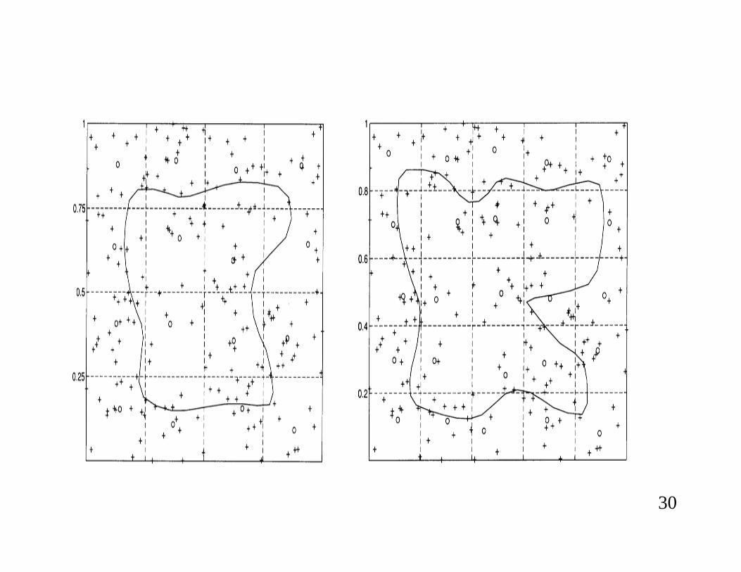
B

C

300

600

500

X

Y

Z

600

300

500

3

flow from plants to warehouses

Supply Demand

04

1

1

73

6

36

A Tabular Representation

Plant x y z Supply 0 4 1 A 300

1 6 3 B 600

3 7 6 C 500

Demand 600 300 500 1400

Warehouse

4

Plant x y z Supply0 4 1A 300

1 6 3B 600

3 7 6C 500

Demand 600 300 500 1400

Ad-Hoc Solution Procedure

1. Avoid the most costly route

2. Fully utilize the cheapest route

300

0

Warehouse

5

0

300 0 0

Ad-Hoc Solution Procedure -- continued

Plant x y z Supply0 4 1A 3001 6 3B 6003 7 6C 500

Demand 600 300 500 1400

Warehouse

0

0

0

300

300 300

0

6

0 0

0

0

Plant x y z Supply0 4 1A 3001 6 3B 6003 7 6C 500

Demand 600 300 500 1400

0

0

500

300300

300

0

0

Ad-Hoc Solution Procedure -- continued

g Total cost = 300 x 0 + 300 x 1 + 300 x 6 + 500 x 6 = $5100

g This approach is reasonable, but a much better solution exists

Warehouse

0 0

7

0

0

00

0

Optimal Solution

WarehousePlant x y z Supply

0 4 1A 300

1 6 3B 600

3 7 6C 500

Demand 600 300 500 1400

0

400

200

0

0

300

300

200

0

g Total cost = 300 x 1 + 400 x 1 + 200 x 3 + 200 x 3 + 300 x 7 = $4000

g Note 1. Nothing is sent along the zero cost route

g Note 2. Most expensive route is used as much as possible

g Note 3. We can obtain this solution using linear programming 8

Observations

g We examined a small, toy problem

g We applied common sense and intuition in our ad hoc solution procedure

g The resulting cost was 27.5% above the cheapest (optimal) cost

g Common sense and intuition were not good enough

g In practice, transportation problems are much larger and need to be solved repeatedly

g If we can’t use linear programming, we should apply a systematic procedure (a heuristic) that consistently generates feasible, near-optimal solutions

g The minimum-matrix method is one such heuristic9

A Small Diversion

g Linear programming (LP) is one of the fundamental tools of management science

g George Dantzig developed the simplex method in 1947

g Dantzig was born in 1914

g His father, Tobias Dantzig, taught in our Math Dept. for many years

g George wrote his dissertation in mathematical statistics at Berkeley

g He worked in the Pentagon during WWII

g He spent many years as a Professor at Stanford

g He received an Honorary Doctorate from us in 1976

g About the 1975 Nobel Prize in Economics 10

Plant x y z Supply0 4 1A 300

1 6 3B 600

3 7 6C 500

Demand 600 300 500 1400

The Minimum-Matrix Method

Warehouse

000300

300

g Find the cheapest routeg Send as much as possible along this route

11

Plant x y z Supply0 4 1A 300

1 6 3B 600

3 7 6C 500

Demand 600 300 500 1400

The Minimum-Matrix Method -- continued

Warehouse

000300

0

300300

12

0

Plant x y z Supply 0 4 1 A 300

1 6 3 B 600

3 7 6 C 500

Demand 600 300 500 1400

The Minimum-Matrix Method -- continued

13

Warehouse

000300

0

300

200

0

00

300

Plant x y z Supply0 4 1A 300

1 6 3B 600

3 7 6C 500

Demand 600 300 500 1400

The Minimum-Matrix Method -- continued

000300

Warehouse

0

0

00

300

14

300 200

00

0

g Total cost = 300 x 0 + 300 x 1 + 300 x 3 + 300 x 7 + 200 x 6 = $4500

g The resulting cost is only 12.5% above the optimal cost

300

Logistics Management

g Logistic management involves the cost-effective flow and storage of goods, services, and personnel from origin to destination according to a set of pre-specified requirements

g The transportation problem is a simple example of logistics management

g The maximum flow, shortest path, and traveling salesman problem are others

15

g A large number of commuters travel from a to g every dayg Three routes are shown below

g Each section of the track (each link) has a capacity (number of trains per hour) based on safety considerations

g Suppose each capacity is 10g How many trains per hour can reach g?g How can the number be increased by changing the capacity of a

single link?

Maximum Flow in a Railway Network

g

fe

d

c

ba

16

Find the Most Economical Package - Delivery Route from San Francisco to New York

5

4

9.5

Seattle

San Francisco

12

4.58

7.5

8.5

5.5

3.5

33

7.5

62.5Salt Lake

City

Houston

Memphis

New YorkChicago

St. Louis

17

The Traveling Salesman Problem

g Imagine a suburban college campus with 140 separate buildings scattered over 800 acres of land

g To promote safety, an experienced security guard must inspect each building every evening

g The goal is to sequence the 140 buildings so that the total time(travel time plus inspection time) is minimized

g This is an example of the well-known TSP

Original problem Possible solution18

g Definitions

h Algorithm – method for solving a class of problems on a computer

h Optimal algorithm – verifiable optimal solutionh Heuristic algorithm – feasible solution

g Performance Measures

h Number of basic computations / Running timeh Computational effort

--- Problem size--- Player one--- Player two

Analysis of Algorithms

19

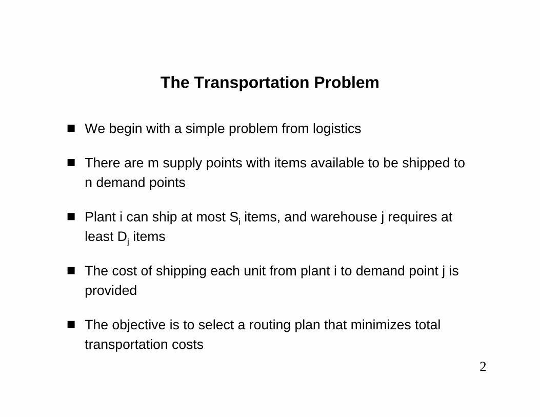
Computational Effort as a Function of Problem Size

20

10

100

1,000

10,000

100,000

1,000,000

10,000,000

0 20 40 60 80 100 120n

Computationaleffort

n

nlog2n

n2

n32n

Problem size

g Terminologyh Researchers have emphasized the importance of finding

polynomial time algorithms, by referring to all such polynomial algorithms as inherently good

h Algorithms that are not polynomially bounded, are labeled inherently bad

g Good Optimal Algorithms Exist for these Problemsh Transportation problemh Maximum flow problemh Shortest path problemh Linear programming

Good vs. Bad Algorithms

21

g Good Optimal Algorithms Don’t Exist for these Problems

h Traveling salesman problem (TSP)

h Complex logistics problems (e.g., vehicle routing, vehicle fleetmanagement, delivery with time-windows, pickup and delivery systems, integration of inventory and transportation)

g Why Focus on Heuristic Algorithms?

h For the above problems, optimal algorithms are not practical

h Efficient, near-optimal heuristics are needed to solve real-world problems

h The key is to find fast, high-quality heuristic algorithms

Good vs. Bad Algorithms -- continued

22

g Aggregate / disaggregate

g Divide and conquer

g Allow uphill moves for minimization problems

Some Heuristic Algorithm Strategies

23

g Find the shortest TSP tour through n points

g Algorithm

h Introduce a rubber band as a small circle around the center of gravity of the points

h Stretch the rubber band towards the points by minimizing an energy function of the form:

where K 0 and

h The rubber band is stretched over time, using ideas from calculus, until the rubber band and the points coincide

The Elastic Net Algorithm[Durbin and Willshaw 87]

24

∑ −β+∑∑α−==

+=

−−

=

m

1j1jj

m

1j

2K2/||jyix||n

1i||yy||elnKE

→ 222

211 )ba()ba(||ba|| −+−=−

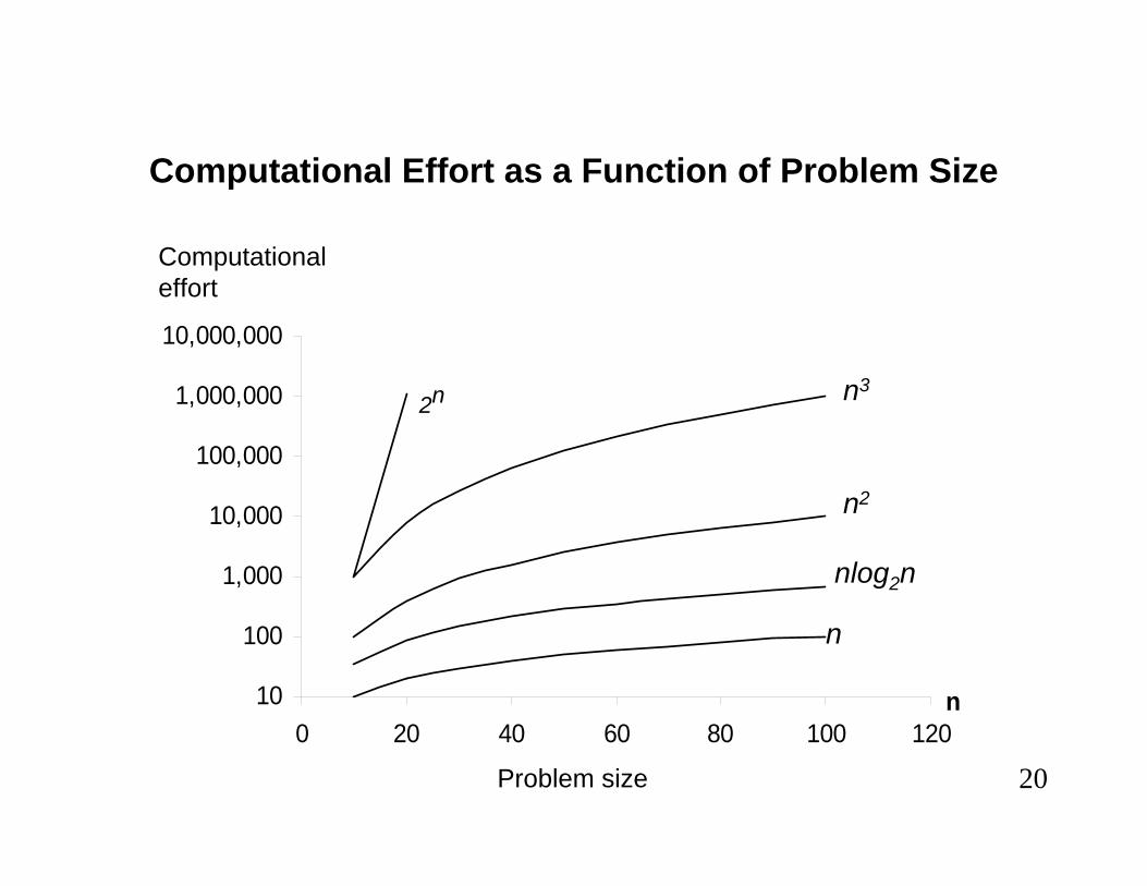
g Explain the two terms of the energy function

g Procedure is iterative

g At each iteration, the most burdensome step involves n x m exponentiations

g To speed up the algorithm, we must address this bottleneck

Key Observations

25

26

The Concept of Rubber Band Points

27

g Reduce both n and m by aggregating the points

g Slowly disaggregate

g Define center of gravity

Aggregation / Disaggregation Strategy

28

29

30

31

32

33

Where Does the Speedup Come From?

Iteration Number Original Elastic Net Accelerated Elastic Net n m n x m n m n x m

1 - 50 500 1250 625,000 4 12 48 51 - 100 500 1250 625,000 9 27 243101 - 150 500 1250 625,000 16 48 768151 - 200 500 1250 625,000 25 75 1875201 - 250 500 1250 625,000 36 108 3888

· · · · · · · · ·

951 - 1000 500 1250 625,000 500 1250 625,000

34

g The approximate speedup for 500 points is 16.4

g The approximate speedup for 1000 points is 17.2

g Impact: 10 minutes vs. nearly 3 hours

g The accelerated elastic net is faster and yields higher quality tours

Practical Observations

35

a. Horizontal bisection b. Subproblems solved

c. Patched solution d. Recursive divide and conquer36

Divide and Conquer

37

Allow Uphill Moves

C A B

Length C

Length B

Length A

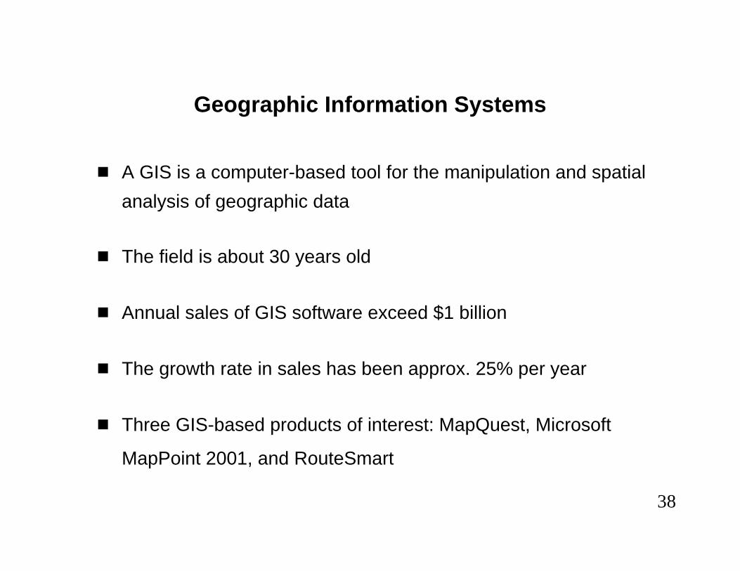
Geographic Information Systems

g A GIS is a computer-based tool for the manipulation and spatial analysis of geographic data

g The field is about 30 years old

g Annual sales of GIS software exceed $1 billion

g The growth rate in sales has been approx. 25% per year

g Three GIS-based products of interest: MapQuest, Microsoft

MapPoint 2001, and RouteSmart

38

RouteSmart Technologies, Inc.

g Company designs and sells vehicle routing and scheduling software

g Small Md. Firm, based in Columbia, founded in 1980

g Owned by a large NY civil engineering company

g I’ve been associated with the firm from the beginning

g Currently run by Larry Levy -- my newspaper boy in 1978 & 1979

g RouteSmart clients include the NY Times, The WSJ, and the San Francisco Chronicle

g RouteSmart has major installations in the newspaper, utility, sanitation, and small package delivery industries

g Larry Levy graduated (B.S. & Ph.D.) from our Business School in the 1980s

39

The Size of the Small Package Delivery Industry

40

g FedEx

h5 million shipments / business dayh55,000 vehicles in the ground fleet

g UPS

h13.1 million packages dailyh150,000 vehicles in the ground fleet

g USPS

h More than 200 billion pieces of mail over 302 delivery daysh 237,000 routes, 6 days a week

Business-to-Consumer Ecommerce

g By 2004, home delivery revenues from B2C ecommerce alone are expected to exceed $125 billion

g Competition among FedEx, UPS, and the USPS is intense

g With express mail, air transportation is key

g FedEx took the early lead and UPS had to play catch-up

g With B2C ecommerce, ground transportation is key

g UPS has the advantage in fleet size and FedEx must play catch-up

41

FedEx Home Delivery and RouteSmart

g FedEx Ground (formerly the RPS Group) focuses on B2B

g Opened Home Delivery in March 2000

g 68 terminals in U.S. currently

g 150 additional terminals to open in 2001

g 20,000 packages / business day (growing steadily)

g Focus on responding to B2C ecommerce

g All packages are routed for delivery using RouteSmart42

Streets Pre-assigned to Routes43

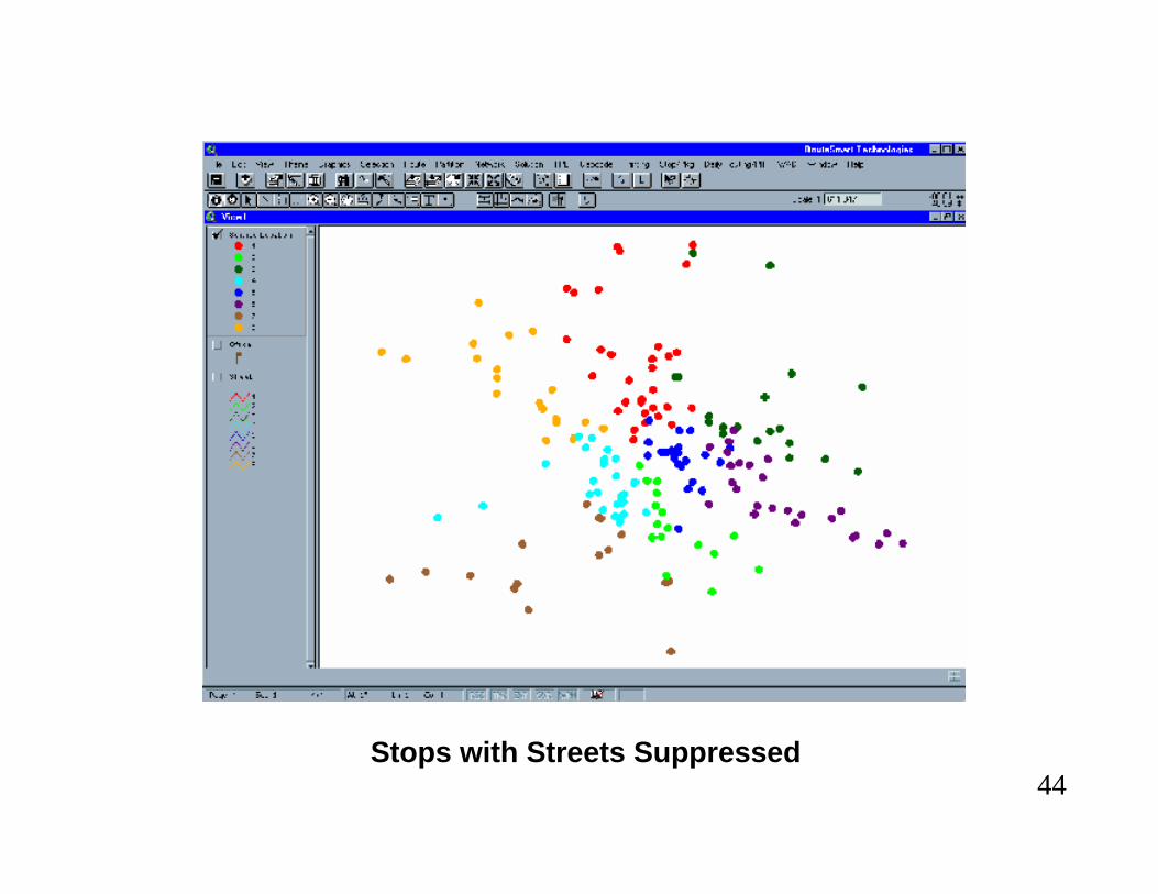
Stops with Streets Suppressed44

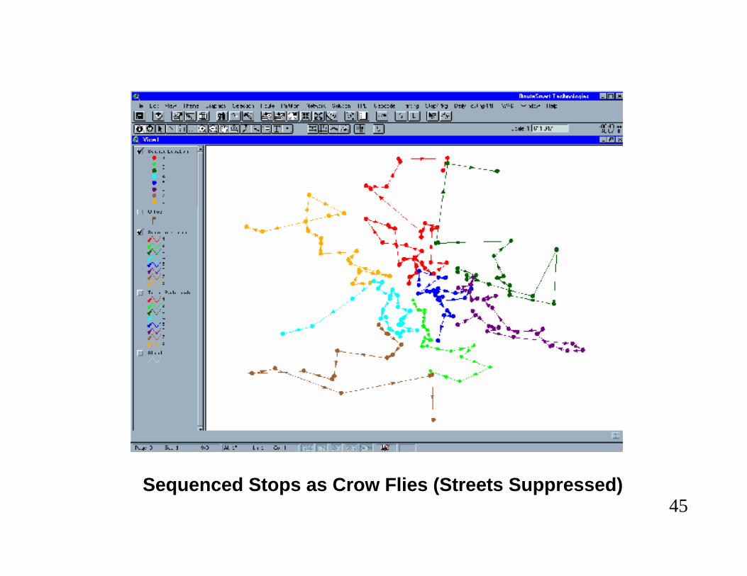
Sequenced Stops as Crow Flies (Streets Suppressed)45

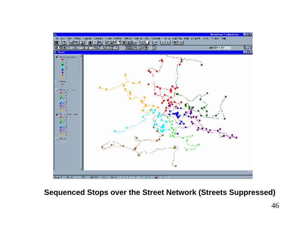
Sequenced Stops over the Street Network (Streets Suppressed)46

Detailed Display of a Single Travel Path (Gray Streets)47

g Logistics and distribution management has often been taken for granted

g This has changed in the last decade or so

g We observed that even “simple” logistics problems can be difficult to solve

g Common sense and intuition are not good enough

g Systematic procedures (e.g., heuristics) often need to be designed and applied

g We discussed several strategies for designing heuristics for solving the TSP

g These strategies can be used to tackle important real-world problems (e.g., the FedEx Home Delivery problem)

g A wide variety of more complex logistics and distribution management problems can be approached in the same way

Conclusions

48

g Coy, Golden, Runger, & Wasil, “ See the Forest before the Trees: Fine-tuned Learning and its Application to the TSP, ” IEEE Trans. on Systems, Man, and Cybernetics (Part A), 28 (4), 454-464 (1998)

g Michalewicz & Fogel, How to Solve It: Modern Heuristics, Springer (2000)

g Rivett, The Craft of Decision Modelling, Wiley (1994)

g Vakhutinsky & Golden, “ A Hierarchical Strategy for Solving TSPs Using Elastic Nets, ” Journal of Heuristics, 1(1), 67-76 (1995)

Recommended Reading

49

g It was given for work in LP, but not to Dantzig

g Instead, it was awarded to Koopmans (Yale) and Kantorovich (USSR)

g Prize was $240K – to be split

g Many were outraged at Dantzig’s omission

g Koopmans considered declining the Prize

g In the end, he accepted the Prize and immediately donated $40K to a Think Tank in Austria with which Dantzig was affiliated

g He was left with $80K (one-third of $240K) which was the most he felt he deserved

Epilogue: The 1975 Nobel Prize in Economics

50