Algorithms and Data Structuresfor Truncated Hierarchical B–splines

Gabor Kiss1, Carlotta Giannelli2, and Bert Juttler2

1 Doctoral Program “Computational Mathematics”2 Institute of Applied Geometry

Johannes Kepler University Linz, Altenberger Str. 69, 4040 Linz, Austriae–mail: gabor.kiss@dk-compmath.jku.at, carlotta.giannelli@jku.at,

bert.juettler@jku.at

Abstract. Tensor–product B–spline surfaces are commonly used as stan-dard modeling tool in Computer Aided Geometric Design and for nu-merical simulation in Isogeometric Analysis. However, when consideringtensor–product grids, there is no possibility of a localized mesh refine-ment without propagation of the refinement outside the region of in-terest. The recently introduced truncated hierarchical B–splines (THB–splines) [5] provide the possibility of a local and adaptive refinement pro-cedure, while simultaneously preserving the partition of unity property.We present an effective implementation of the fundamental algorithmsneeded for the manipulation of THB–spline representations based onstandard data structures. By combining a quadtree data structure —which is used to represent the nested sequence of subdomains — with asuitable data structure for sparse matrices, we obtain an efficient tech-nique for the construction and evaluation of THB–splines.

Keywords: hierarchical tensor–product B–splines; truncated basis; THB–splines;isogeometric analysis; local refinement

1 Introduction

The de facto standard in computer aided geometric design is the tensor–productB–spline model together with its non–uniform rational extension (NURBS).Among other fundamental properties, like minimum support, efficient refine-ment and degree–elevation algorithms, B–splines are nonnegative and form apartition of unity. This implies that a B–spline curve/surface is completely con-tained in the convex hull of a certain set of points, usually referred to as controlnet. The shape of the control net directly influences the shape of the B–splinerepresentation, so that the designer can use it to manipulate the correspondingparametric representation in a fairly intuitive way. Unfortunately, an unavoid-able drawback of the tensor–product structure is a global nature of the meshrefinement which excludes the possibility of a local refinement scheme as illus-trated in Figure 1(a–c).

2

(a) initial grid (b) area of interest (c) knot insertion (d) hierarchical grid

Fig. 1. Adaptive refinement of an initial tensor–product grid (a) with respect to alocalized region (b) may be achieved by avoiding a propagation of the refinement dueto the tensor–product structure (c) through a hierarchical approach (d).

Despite an increasing interest in the identification of adaptive spline spacesand related applications, see e.g., [7, 15, 18], local mesh refinement remains anon–trivial and computationally expensive issue. A suitable trade–off betweenthe quality of the geometric representation (in terms of degrees of freedom neededto obtain a certain accuracy) and the complexity of the mesh refinement algo-rithm has necessarily to be taken into account. Different approaches have beenproposed which all extend the standard tensor–product model by allowing T–junctions between axis aligned mesh segments. Among others, this led to the in-troduction of hierarchical B–splines (HB–splines) [4, 11, 12], T–splines [16], poly-nomial splines over T–meshes [2] and – more recently – truncated hierarchicalB–splines (THB–splines) [5] and locally refined B–splines [3].

The idea of performing surface modeling by manipulating the parametricrepresentation at different levels of details was originally proposed by Forsey andBartels [4]. In order to localize the editing of detailed features, the refinementis iteratively adapted on restricted patches of the surface in terms of a sequenceof overlays with nested knot vectors. Subsequently, Kraft [11, 12] showed thatthe hierarchical structure enforced on the mesh refinement procedure can becomplemented by a simple and automatic identification of basis functions whichnaturally generalizes some of the fundamental properties of tensor–product B–splines — such as nonnegativity and linear independence — to the case of HB–splines.

The multilevel approach allows to break the rigidity of a tensor–productconfiguration by simultaneously preserving a highly organized structure as shownin Figure 1(d). An example of hierarchical refinements over rectangular–shaperegions is presented in Figure 2.

The hierarchical B–spline model found applications in data interpolation andapproximation [10, 11, 13], as well as in finite element and isogeometric analysis[1, 14, 18]. Alternative spline hierarchies were also considered in the literature,see e.g., [9, 19].

Kraft’s basis for HB–splines does not possess the partition of unity prop-erty without additional scaling and it possesses only limited stability properties.

3

Truncated hierarchical B–splines [5] have the potential to overcome these lim-itations and provide improved sparsity properties. They were introduced as apossible extension of normalized tensor–product B–splines to suitably handlethe local refinement in adaptive surface approximation algorithms. This multi-level scheme was also generalized and further investigated in [6], where particularattention was devoted to the stability analysis of the proposed hierarchical con-struction.

In virtue of the multilevel nature of the hierarchical B–spline approach, thenatural choice in terms of data structures is a tree–like representation wherea given refinement level correspond to a certain level of depth in the tree [4].Related and alternative solutions were also further investigated. An algorithm forscattered data interpolation and approximation by multilevel bicubic B–splinesbased on a hierarchy of control lattices was described in [13]. An implementationof hierarchical B–splines in terms of a tree data structure whose nodes representthe B–splines from different levels was recently presented in [1]. Another solutionconsists of storing in each node of the tree the data related to a knot span of acertain level, in particular the significant basis functions acting on it [14].

The goal of the present paper is to introduce an effective implementationof data structures and algorithms for the newly introduced THB–splines. Torepresent the subdomain hierarchy we use a quadtree data structure in com-bination with sparse matrices. The quadtree provides an efficient and dynamicdata structure for representing the subdomains. It also facilitates the neededupdate which may be caused by an iterative refinement process. One key moti-vation for this choice is to reduce the memory overhead in need for storing thesubdomain hierarchy as much as possible. The selection of (possibly truncated)basis functions proceeds as described in [5] by means of certain queries whichuse the quadtree. The result is encoded by a sequence of sparse matrices. Thequadtree and the related sparse matrices are initially created and subsequentlyupdated during the refinement procedure. For the hierarchical spline evaluationalgorithm, however, only the access to the sparse matrices is required. This leadsto a reasonable trade–off with respect to memory and time consumption duringboth the construction of THB–splines from an underlying subdomain hierarchyand their evaluation for given parameter values.

The paper is organized as follows. In Section 2 we describe the hierarchicalapproach to adaptive mesh refinement together with the definition and eval-uation of the THB–spline basis. Section 3 introduces the data structures andalgorithms used for the representation of the subdomain hierarchy, while Sec-tion 4 explains the construction of the matrices needed during the THB–splineevaluation in more detail. Some numerical results are then presented in Section 5to illustrate the performance of our approach, while the extension of the pro-posed approach to more general knot configurations and refinements is discussedin Section 6. Finally, Section 7 concludes the paper.

4

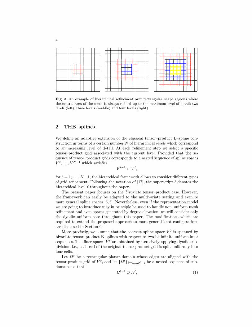
Fig. 2. An example of hierarchical refinement over rectangular–shape regions wherethe central area of the mesh is always refined up to the maximum level of detail: twolevels (left), three levels (middle) and four levels (right).

2 THB–splines

We define an adaptive extension of the classical tensor–product B–spline con-struction in terms of a certain number N of hierarchical levels which correspondto an increasing level of detail. At each refinement step we select a specifictensor–product grid associated with the current level. Provided that the se-quence of tensor–product grids corresponds to a nested sequence of spline spacesV 0, . . . , V N−1 which satisfies

V `−1 ⊂ V `,

for ` = 1, . . . , N−1, the hierarchical framework allows to consider different typesof grid refinement. Following the notation of [17], the superscript ` denotes thehierarchical level ` throughout the paper.

The present paper focuses on the bivariate tensor–product case. However,the framework can easily be adapted to the multivariate setting and even tomore general spline spaces [5, 6]. Nevertheless, even if the representation modelwe are going to introduce may in principle be used to handle non–uniform meshrefinement and even spaces generated by degree elevation, we will consider onlythe dyadic uniform case throughout this paper. The modifications which arerequired to extend the proposed approach to more general knot configurationsare discussed in Section 6.

More precisely, we assume that the coarsest spline space V 0 is spanned bybivariate tensor–product B–splines with respect to two bi–infinite uniform knotsequences. The finer spaces V ` are obtained by iteratively applying dyadic sub-division, i.e., each cell of the original tensor-product grid is split uniformly intofour cells.

Let Ω0 be a rectangular planar domain whose edges are aligned with thetensor-product grid of V 0, and let Ω``=0,...,N−1 be a nested sequence of sub-domains so that

Ω`−1 ⊇ Ω`, (1)

5

(a) Ω0 ⊇ Ω1 (b) Ω0 ⊇ Ω1 ⊇ Ω2 (c) Ω0 ⊇ Ω1 ⊇ Ω2 ⊇ Ω3

(d) Ω0 ⊇ Ω1 (e) Ω0 ⊇ Ω1 ⊇ Ω2 (f) Ω0 ⊇ Ω1 ⊇ Ω2 ⊇ Ω3

Fig. 3. Two nested sequences of subdomains — indicated as linear (top) and curvilinear(bottom) in Example 1. They satisfy relation (1) with respect to two (left), three(middle) and four (right) hierarchical levels.

for ` = 1, . . . , N − 1. Each Ω` is defined as a collection of cells with respect tothe tensor–product grid of level `− 1.

Example 1. Figures 2 and 3 show three subdomain hierarchies which will beused to demonstrate the performance of our algorithms and data structures:

– rectangular (refinement over rectangular–shaped regions);– linear (refinement along a diagonal layer);– curvilinear (refinement along a curvilinear trajectory).

By starting with an initial tensor–product configuration at level 0, the tensor–product grid associated with level `+1 is obtained by subdividing any cell of theprevious level into four parts. Each subdomain Ω` is then defined as a certaincollection of cells with respect to the grid of level ` so that (1) is satisfied. Figure 2illustrates an example of hierarchical refinement over rectangular–shape regionswhere the central area of the mesh is always refined up to the maximum levelof detail. The other two subdomain hierarchies mentioned above are shown inFigure 3 up to four refinement levels so that Ω0 ⊇ . . . ⊇ Ω3.

For each hierarchical level `, with ` = 0, . . . , N − 1, let B` be the normalizedB–spline basis of the spline space V ` with respect to a certain degree (d, d)

6

defined on corresponding nested knot sequences. We say that

β ∈ B` is active ⇔ supp0 β ⊆ Ω` ∧ supp0 β 6⊆ Ω`+1,

where supp0 β = suppβ ∩ Ω0 is a slightly modified support definition whichmakes local refinements possible also along the boundaries of Ω0. A B–splineβ ∈ B` is then active if it is completely contained in Ω` but not in Ω`+1, andpassive otherwise.

We may assume the initial domainΩ0 to be an axis-aligned box3. By denotingwith k the number of knot spans of level 0 along the edges ofΩ0, which is assumedto be the same for both directions, we define a characteristic matrix X` of sizes` × s`, with s` = (2`k + d), for ` = 0, . . . , N − 1. These matrices collect theinformation about active/passive B–splines level by level, namely

X`i,j =

1 if β`i,j is active,0 otherwise,

where β`i,j is a B–spline of level `. The indices i, j are chosen such that exactly

the B-splines β`i,j with i, j = 1, . . . , s` are non–zero on Ω0.

Definition 1 ([11, 12], extended in [18]). The hierarchical B–spline (HB–spline) basis H is defined as the set of all active B–splines defined over thetensor–product grid of each level,

H =⋃

`=0,...,N−1

β`i,j ∈ B` : X`i,j = 1.

A spline function represented in the hierarchical B–spline basis is then definedas a linear combination of active B–splines from different levels in the hierarchy.In order to evaluate the considered spline in a given point of the domain, thecontribution of all the active B–splines (from the minimum to the maximum levelof basis functions whose support is non–zero on that point) has to be computedand then added together. The cost of the hierarchical evaluation algorithm isthen quadratic and linear with respect to the degree (B–spline evaluation) andthe number of levels, respectively.

Truncated hierarchical B–splines [5, 6] form a different basis for the samemultilevel B–spline space. The key idea behind this alternative hierarchical con-struction is to properly exploit the refinable nature of the B–spline basis whichallows to express a B–spline of level ` in terms of (d+2)2 functions which belongto level ` + 1 and of certain binomial coefficients scaled by a factor 2−d withrespect to any dimension. By using this subdivision rule, any function τ ∈ V `can be represented according to a two–scale relation with respect to the basisB`+1 of V `+1, namely

τ =∑

β∈B`+1

c`+1β (τ)β,

3 Different shapes are easily identified at subsequent levels as shown in Figure 3.

7

with certain coefficients c`+1β (τ) ∈ R. The truncation of τ ∈ V ` with respect to

B`+1 and Ω`+1 is the function trunc`+1τ ∈ V `+1 defined as:

trunc`+1τ =∑

β∈B`+1,supp β 6⊆Ω`+1

c`+1β (τ)β.

The overall truncation of a hierarchical B–spline β ∈ B` ∩H is defined by recur-sively applying the truncation with respect to the different levels,

truncβ = truncN−1(truncN−2 . . . (trunc`+1β)).

By recursively discarding the contribution of active B–splines of subsequent lev-els from coarser B–splines, we obtain the definition of the truncated basis.

Definition 2 ([5]). The truncated hierarchical B-spline (THB–spline) basis Tis defined by

T =truncβ`i,j : X`i,j = 1, ` = 0, . . . , N − 2 ∪ βN−1i,j : XN−1

i,j = 1.

Truncated hierarchical B–spline are linearly independent, non-negative, forma partition of unity and preserve the nested nature of the spline spaces [5].Moreover, the construction of THB–splines is strongly stable with respect tothe supremum norm provided that the knot vectors satisfy certain reasonableassumptions — see [6] for more details.

In addition to the characteristic matrices X`N−1`=0 , we consider another se-

quence of matrices C`N−1`=0 of the same size and with the same sparsity pattern,i.e. X`

i,j = 0 implies c`i,j = 0. These matrices store the coefficients associated tothe (active) basis functions in the representation of a spline function with respectto the truncated basis. The following simple algorithm performs the evaluationof a hierarchical spline function which is represented in terms of THB–splines.

Algorithm EVAL THB(seqmat X, seqmat C, int D, int LMAX, float U,V)

\\ seqmat X is the sequence of characteristic matrices, i.e., X[L] is the char-acteristic matrix of level L

\\ seqmat C is the sequence of coefficient matrices associated to the splinefunction f , i.e., C[L] is the coefficient matrix of level L

\\ int D is the degree in both directions\\ int LMAX is the maximum refinement level N − 1\\ float U,V are evaluation parametersIdentify the (D+1)×(D+1) sub–matrix M of C[0] which contains the coeffi-

cients of those B–splines of level 0 that are non–zero at (U,V)for L = 1 to LMAX do

Generate the matrix S by applying one step of B–spline subdivision to M

Identify the (D+1)×(D+1) sub–matrix T of S which contains the coeffi-cients of those B–splines of level L that are non–zero at (U,V)

for each pair of indices i,j in T do

if X[L](i,j) == 1 then T(i,j) = C[L](i,j)

8

M = T

return the value f obtained by applying de Boor’s algorithm to M

In this algorithm, the sub-matrices M,S, and T at a certain level are al-ways accessed by global indices, i.e., indices with respect to the entire arrayof all tensor–product splines of that level. The following proposition clarifiesthe connection between the evaluation algorithm and the truncated hierarchicalB–spline basis.

Theorem 1. The value f(u, v) computed by the algorithm is the value of afunction represented in the THB–spline basis.

This can be proved by applying the algorithm to Kronecker–type coefficientdata, where exactly one coefficient is nonzero and equals 1. This corresponds tothe evaluation of a truncated basis function.

The cost of the THB–spline evaluation algorithm EVAL_THB is equal to N −1times the application of the B–spline subdivision rule plus the cost due to thestandard de Boor’s algorithm. Consequently, it grows linearly with the numberof levels and quadratically with the degree of the splines. This is similar to thecosts needed for evaluating the classical (non-truncated) hierarchical B–splines.The computational cost could be further reduced

– by starting the for loop at the minimum level of functions which are activeat the given point (u, v), and

– by stopping it at the maximum level of functions which are active at thispoint.

With this modification, the computational costs grows linearly with the numberof levels which are active at the given point. This number can be controlled bychoosing a suitable refinement strategy.

The following sections discuss data structures and algorithms for manipulat-ing and storing the subdomain hierarchy and for representing the characteristicmatrices and coefficient matrices.

3 Representing and manipulating the subdomainhierarchy

The domain Ω0 is now assumed to be a box consisting of 2n × 2n cells of thecoarsest tensor-product grid, where n is a non-negative integer. This assumptionis made in order to facilitate the use of a quadtree data structure. Moreover, inorder to simplify the implementation, the edges of the coarsest tensor–productgrid should have the length 2M−1, where M is the maximum number of lev-els, i.e. N ≤ M . Under this assumption, all coordinates of bounding boxes inthe algorithms presented below are integers. Alternatively, one may use otherexact data types than integers (e.g. rational numbers), thereby eliminating therestriction on the number of levels.

9

3.1 The subdomain hierarchy quadtree

We represent the entire subdomain hierarchy by a single quadtree. Each node ofthe quadtree takes the form

struct qnode

aabb box;

int level;

*node nw;

*node ne;

*node sw;

*node se; ;

where the axis–aligned bounding box aabb box is characterized by coordinatesof its upper left and lower right corner, level defines the highest level in whichthe box is completely contained and nw, ne, sw, se are pointers to the fourchildren of the node. These children represent the northwestern, northeastern,southwestern and southeastern part of the box after the dyadic subdivision. Allpointers to these children are set to null until the node is created during theinsertion process, which is described by the INSERTBOX algorithm below.

LetΩ` =⋃i b`i , where each b`i is a collection of cells forming a rectangular box.

During the creation of the quadtree which represents the subdomain hierarchy,for each level `, we insert all boxes b`i which define Ω`. The following recursivealgorithm performs the insertion of a box b`i into the quadtree:

Algorithm INSERTBOX(box B, qnode Q, int L)\\ box B is the box which will be inserted\\ qnode Q is the current node of the quadtree\\ int L is the levelif B == Q.box then

Q.level = L

visit all nodes in the subtree with root Q; if the level of a node is lessthan L then increase it to L

else

for child in Q.nw, Q.ne, Q.sw, Q.se do

if child != null then

If B∩Q.box 6= ∅ then INSERTBOX(B∩Q.box, child, L)

else

create the box childbox of childif B∩childbox 6= ∅ then

create the node child

set child.box to childbox, child.level to Q.level and thefour children to null

INSERTBOX(B∩childbox, child, L)

After each box insertion we perform a cleaning step, visiting all sub–treesand deleting those where all nodes have the same level. This reduces the depthof the tree to a minimal value and optimizes the performance of all algorithms.

10

Fig. 4. Initial subdomain structure (left) and corresponding quadtree (right) whichstores the boxes related to level 0 and 1 in the hierarchy. The box b = [16, 8] × [24, 12](red) has to be inserted into the quadtree at level 2.

Example 2. To explain the INSERTBOX algorithm, we consider the subdomainhierarchy composed of three levels (N = 3), two of which (level 0 and 1) areinitially present. This is shown in Figure 4, together with the related quadtreerepresentation. The domain Ω0 has k = 16 edges of length 2N−2 = 2. The boxb = [16, 8]× [24, 12] will be inserted at level 2 into the hierarchy. The cells withrespect to the tensor–product grid of level 1 covered by b are depicted in red inFigure 4.

The execution of the algorithm is illustrated in Figure 5. At each step, wehighlight the current node Q and the corresponding box in the subdomain hi-erarchy (Figure 5, right and left column, respectively). The insertion starts byconsidering the root of the tree, where the box b is compared with the axis–aligned bounding box stored in the root. Since these two boxes are not thesame, the level of the root remains unchanged.

Subsequently, we have to identify which boxes between the ones stored inthe four children of the root overlap with b, see Figure 5(a). In this case b iscompletely contained in the box represented by the ne child of the root. Therecursive call of INSERTBOX is therefore applied to this child only. The situationin Figure 5(b) is similar to the previous case. After the split, the algorithm isrecursively applied to the sw child.

In the third step shown in Figure 5(c) instead, the box b overlaps with theboxes related to two children (nw and ne) of the current node. Then, b is alsosubdivided and the recursion is called on both children.

Figure 5(d) shows the last step executed by the insertion of the box b. Twonew nodes are created and inserted into the quadtree. Since these nodes coincidewith the two parts of b, we set their level to 2. Clearly, the box to be inserteddoes not necessarily become a single node of the quadtree but it may be storedinto several nodes.

11

(a) first split (left) and quadtree (right)

(b) second split (left) and quadtree (right)

(c) third split (left) and quadtree (right)

(d) two new boxes (left) are inserted into the quadtree (right)

Fig. 5. Different steps performed by the INSERTBOX function to insert the box b =[16, 8] × [24, 12] into the subdomain hierarchy of Figure 4. The subsequent splits areshown on the subdomain hierarchy (blue lines on the left) with respect to the visit ofthe quadtree (right).

12

3.2 Queries

In order to create the characteristic matrices introduced in Section 2, we definethree query functions on the quadtree. These queries allow to understand if allbasis functions β of a certain hierarchical level whose support is contained in agiven box b are active or passive.

Given a box b defined as a collection of cells with respect to the tensor–product grid of level `, the first query (QY1), returns true if

b ⊆ Ω` ∧ b ∩Ωi = ∅, i > `. (2)

Thus, if QY1 returns true, then all the basis functions of level ` whose supportis completely contained in the box b are active, i.e., they are present in thehierarchical spline basis.

If the second query QY2 returns true then all the basis functions of level `whose support is contained in the box b are passive, i.e., they are not present inthe hierarchical spline basis. This is characterized by the following condition:

b ∩Ω` = ∅ ∨ b ⊆ Ω`, for some i > `. (3)

The third query QY3 returns the highest level ` with the property that Ω`

contains the box b.All the three queries can easily be implemented with the help of the quadtree

structure described before. In particular, the structure of queries QY1 and QY2

is similar. We visit the quadtree until we find a leaf node or a node where theresult of the query changes from to true to false. At that point, we can concludethe visit and return false. On the other hand, query QY3 requires a complete visitof the quadtree.

Example 3. Figure 6(b–d) shows the results of the three queries with respectto the subdomain hierarchy composed of two levels (level 0 and 1) shown onFigure 6(a) for four sampled boxes of level 0. Figures 6(b) and (c) display theresults of QY1 and QY2 for ` = 0, respectively. The boxes in green correspond to apositive answer to the query, the red boxes to a negative one. Finally, Figure 6(d)shows the results for QY3. The green boxes correspond to answer 1 and the redones to answer 0.

4 Characteristic matrices

The characteristic matrices identify the tensor–product basis functions whichare present in the hierarchical basis.

4.1 Creating characteristic matrices

By using the quadtree structure defined in Section 3, we can generate the charac-teristic matrices introduced in Section 2 to represent and evaluate THB–splines.For the creation of these matrices we considered two different approaches:

13

(a) level 0 and 1 (b) QY1 for level 0 (c) QY2 for level 0 (d) results of QY3

Fig. 6. Results of the three queries functions with respect to a subdomain hierarchy(a) with two levels. In case of QY1 (b) and QY2 (c), the green/red boxes correspond to apositive/negative answer. QY3 (d) returns 1 for the green boxes and 0 for the red ones.

– the one–by–one approach where we determine the entries of the characteristicmatrices one by one by applying QY3 to each single basis function;

– the all–at–once approach where we try to set as many values as possible inone single step. This requires a more sophisticated algorithm.

During the creation of the characteristic matrices by the all–at–once ap-proach, we try to set many entries of the matrices at the same time. In order todo this, the query functions are initially called for boxes which cover the initialdomain Ω0. The SETMAT algorithm below creates the characteristic matrices forall subdomains in the subdomain hierarchy.

Algorithm SETMAT(qnode Q, seqmat X)

\\ qnode Q is the root of the quadtree which stores the subdomain hierarchy\\ seqmat X is the sequence of characteristic matrices, i.e. X[L] is the char-acteristic matrix of level Lfor all levels L do

Create the index set I for all functions of level L acting on Ω0. I is anaxis-aligned box in index space.

SETBOX(B,X[L])

SETMAT calls the algorithm SETBOX. When the answer active/passive cannotbe given for the current call, the considered box is split into 4 disjoint axis–aligned bounding boxes and SETBOX function is recursively applied to them.

Algorithm SETBOX(aabbis I, mat XL)

\\ aabbis I is an axis-aligned box in index space\\ mat XL is a characteristic matrix of level LThe level L is a global variableCreate the axis-aligned bounding box B covering all cells of level L which

belong to the supports of functions with indices in I

if QY1(B, L) then

for all indices (i,j) in I do XL[i,j]=1

14

(a) (b) (c) (d) (e) (f)

Fig. 7. A subdomain hierarchy with two levels and some of the boxes I in index space(shown as circles) along with the associated bounding boxes B in parameter space (grey)considered by SETBOX when creating the characteristic matrix X0 for this subdomainhierarchy (a–e). Active (green) and passive (red) functions of level 0 (f).

elseif QY2(B, L) then

for all indices (i,j) in I do XL[i,j]=0

elseif I is a single pair (i,j) then

k = QY3(B, L)

if k == L then XL[i,j]=1

else XL[i,j]=0

else

split I into 4 disjoint axis-aligned bounding boxes I1-I4 by subdividingeach edge (approximately) into halves in index space.

Apply SETBOX to I1-I4 and XL

Example 4. Figure 7 shows a subdomain hierarchy with two levels, consisting ofa square Ω0 and a subdomain Ω1 in the southeastern corner, which is shownin blue. The four pictures (a–e) visualize several index sets I (shown by circles)and the associated boxes B (grey) which are considered by SETBOX when creatingX0 for biquadratic splines.

Initially, SETBOX considers the entire set of basis functions (a) and concludesthat it has to be subdivided. The northwestern subset is shown in (b). QueryQY1 returns 1, therefore the functions are all active; no subdivision is needed.The northeastern and southwestern subsets (not shown) are dealt with similarly.The southeastern subset (c), however, has to be subdivided. Considering itsnorthwestern subset (d) does not lead to a conclusion again, needing anothersubdivision. The functions in this index set have to be analyzed one-by-one(not shown). The northeastern and southwestern subsets (not shown) are dealtwith similarly. For the southeastern subset (e), however, query QY2 returns 1,therefore the functions are all passive. Finally, the procedures arrives at thecorrect classification of basis functions of level 0 (f).

As Example 5 shows the all–at–once approach is not necessarily faster com-pared to the one–by–one mentioned at the beginning of this section. However,the approach becomes considerably faster with an increasing number of levels.This is demonstrated by the next example.

Example 5. Figure 8 compares the all–at–once setting with the one–by–onemethod. The number of queries called by the one-by-one approach is the same

15

0 0.5 1 1.5 2 2.5 3 3.5

x 105

0

1

2

3

4x 10

5

number of basis functions

nu

mb

er

of

qu

erie

s c

alle

d

Fig. 8. The plot visualizes the number of queries needed to create the characteristicmatrices for the three examples in Figure 2, 3 and 9. Compared to the all–at–onceapproach (cyan: linear, green: curvilinear, red: square-shaped refinement), the one–by–one approach (blue: same for all examples) is faster for small numbers of levels andbasis functions, but it becomes slower for higher ones.

Fig. 9. The three subdomain hierarchies considered in Example 6: rectangular (left),linear (middle) and curvilinear (right) refinement, all with six levels.

for the three hierarchical refinements in Figure 9 since it depends solely on thenumber of basis functions. This approach is faster for small numbers of basisfunctions, which typically correspond to a small numbers of hierarchical levels.On the other hand, the all–at–once approach becomes faster for higher numbersof basis functions in all the three considered cases since the number of queriesgrows sub–linearly with respect to the number of basis functions.

4.2 Using sparse data structures

The representation of THB–splines in terms of characteristic matrices allowsa fast look–up during the evaluation process and a simple update of the val-ues when the underlying subdomain hierarchy changes. The drawback of thisrepresentation is the rather large memory consumption, which can exceed the

16

available physical memory even for relatively small meshes and low numbers oflevels. Indeed, it grows exponentially with the number of levels.

This problem can be solved by using a suitable sparse matrix data struc-ture. For our experiments, we chose the compressed sparse column (CSC) datastructure. The nonzero elements (read first by column) are stored in a one–dimensional array. A second array stores the row indices corresponding to thesevalues and a third one collects the indices into the first two arrays of the leadingentry in each column [8].

As detailed in the next section, the CSC structure significantly reduces thememory consumption of our approach (see Example 6). In fact, we will observethat the memory consumption grows linearly with the number of degrees offreedom, instead of exponentially with the number of levels. In addition, theprice paid for reducing the memory requirements is only a small increase of thecomputational time (see Examples 7 and 8).

5 Examples

We implemented the proposed algorithms and data structures in C++. For themanipulation of the characteristic matrices we used the sparse MATLAB rep-resentation in terms of the compressed sparse column approach mentioned atthe end of the previous section. The experiments have been performed on a lap-top running the Windows 7 operating system (Intel Core I5-2520 2.5GHz, 4GBRAM, 64 bit).

Example 6. We compare the memory consumption of full characteristic matriceswith the memory consumption of the matrices represented in the CSC structurefor the three subdomain hierarchies in Figure 9 (rectangular, linear, and curvi-linear).

The experimental results in Figure 10 show that the memory needed by thesparse matrix data structure is considerably smaller then the one related tothe full matrix representation. Moreover, the memory consumption grows onlylinearly with the numbers of degrees of freedom instead of exponentially withthe number of levels. This is the optimal result that one can expect, since acoefficient for each active basis function needs to be stored anyway.

We observe a difference between the results related to the rectangular–shapedrefinement with respect to the linear and curvilinear case. The reason is the dif-ferent nature of the refinement procedure. In the linear and curvilinear case, therefined area is reduced at each new level and the coarser levels do not change (seeFigure 3). In the rectangular case, the refined area of the highest level is constantand the size of lower level subdomains increases (see Figure 2). Thus, using thesparse data structure does not decrease the order of memory consumption inthis case, since the number of degrees of freedom grows exponentially with thenumber of levels.

The next example analyzes the influence of using the sparse data structuresto the time needed to evaluate the multilevel spline functions using the algorithmEVAL_THB.

17

102

103

104

105

105

degrees of freedom

mem

ory

in b

yte

s

102

103

104

105

degrees of freedom

mem

ory

in b

yte

s

102

103

104

105

mem

ory

in b

yte

s

degrees of freedom

Fig. 10. Memory needed to represent the characteristic matrices without (blue) andwith (green) the use of sparse data structures for different numbers of degrees of freedomrelated to the square (top left), the circle (top right) and the line refinement (bottom)refinement. The dashed red line has slope 1 and indicates linear growth.

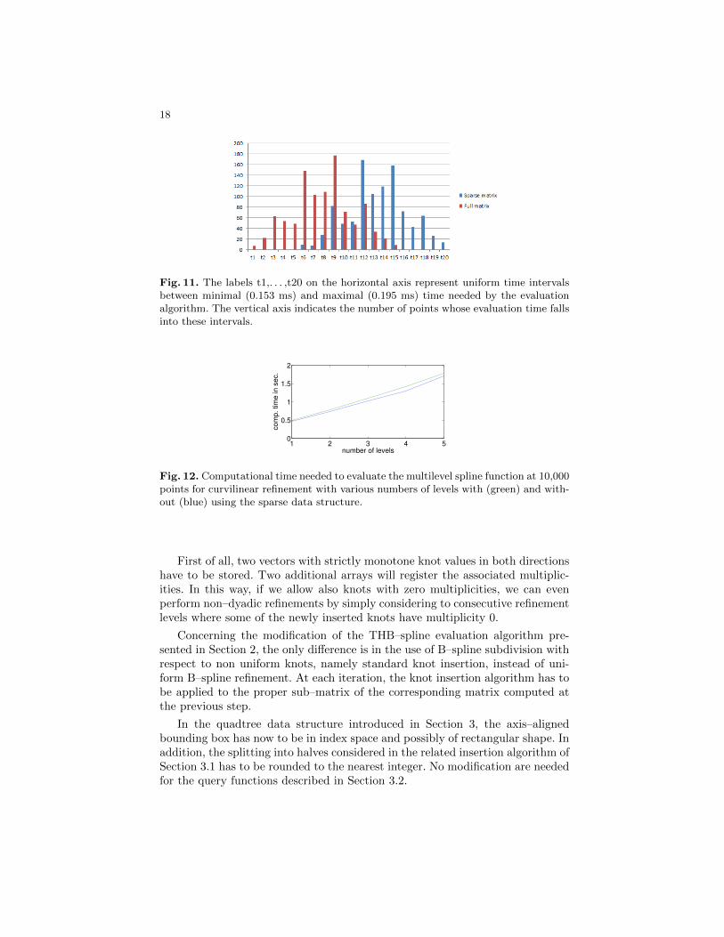
Example 7. Figure 11 visualizes the distribution of the computation times neededto evaluate the multilevel spline function at 1000 points with (blue bars in theplot) and without (red bars in the plot) the use of sparse data structures for thelinear refinement shown in Figure 9. Two facts can be observed:

– the evaluation time does not depend significantly on the location of the pointwith respect to the subdomain hierarchy;

– using the sparse data structure increases the evaluation time only by a verysmall amount.

Note that the evaluation times in this example vary between 0.153 and 0.195milliseconds.

Finally we analyze the relation between evaluation time and the number oflevels in the hierarchy.

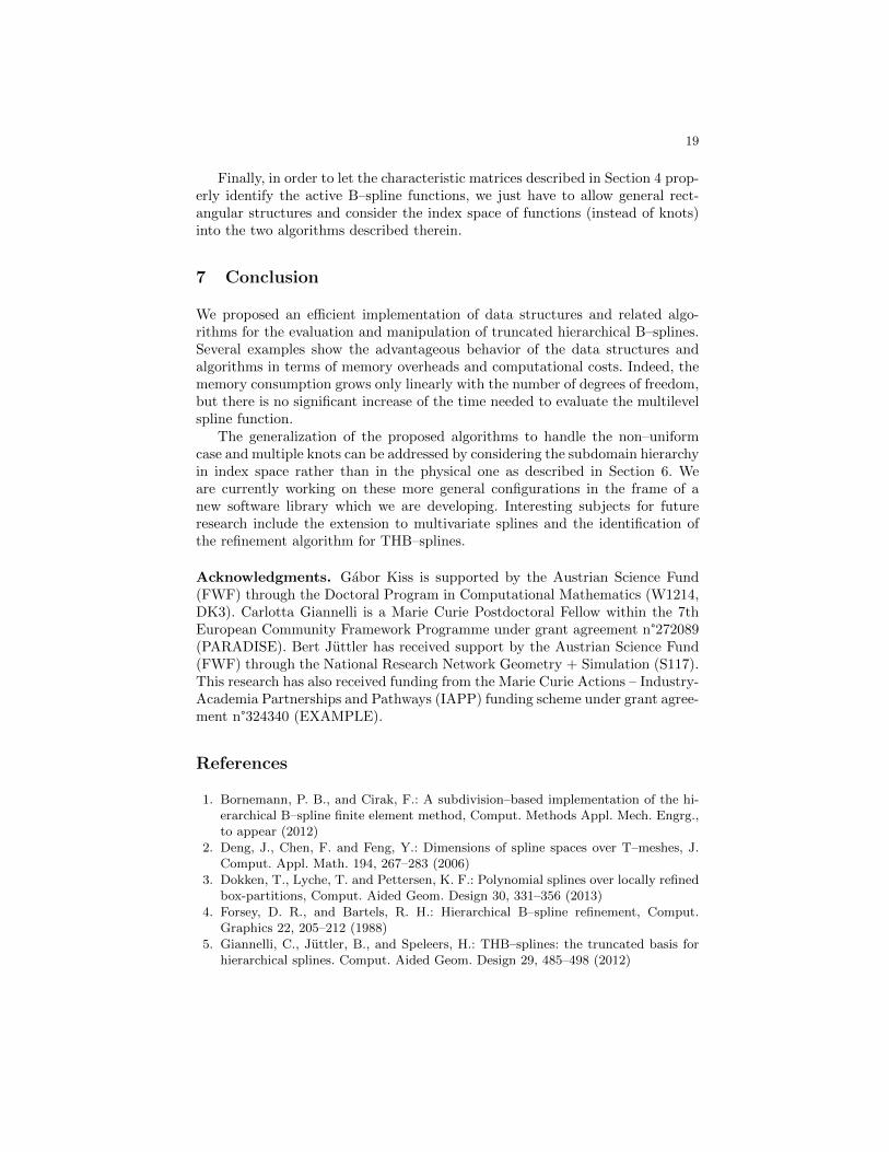
Example 8. We consider the curvilinear refinement shown on the right of Fig-ure 9. Figure 12 compares the evaluation times for 10,000 parameters obtainedby using either the full or the sparse matrix representation. We may note thatthe computational time grows linearly with the increasing level of refinementfor both representations, with a small overhead caused by using the sparse datastructure. The values do not include the time necessary for creating the corre-sponding data structures, only the evaluation algorithm EVAL_THB is considered.

6 Non–uniform knots and general refinement

In order to discuss more general knot configurations, we now describe the mod-ifications of data structures and algorithms which are required to extend theframework to non–uniform knots and different multiplicities.

18

Fig. 11. The labels t1,. . . ,t20 on the horizontal axis represent uniform time intervalsbetween minimal (0.153 ms) and maximal (0.195 ms) time needed by the evaluationalgorithm. The vertical axis indicates the number of points whose evaluation time fallsinto these intervals.

1 2 3 4 50

0.5

1

1.5

2

number of levels

com

p. tim

e in s

ec.

Fig. 12. Computational time needed to evaluate the multilevel spline function at 10,000points for curvilinear refinement with various numbers of levels with (green) and with-out (blue) using the sparse data structure.

First of all, two vectors with strictly monotone knot values in both directionshave to be stored. Two additional arrays will register the associated multiplic-ities. In this way, if we allow also knots with zero multiplicities, we can evenperform non–dyadic refinements by simply considering to consecutive refinementlevels where some of the newly inserted knots have multiplicity 0.

Concerning the modification of the THB–spline evaluation algorithm pre-sented in Section 2, the only difference is in the use of B–spline subdivision withrespect to non uniform knots, namely standard knot insertion, instead of uni-form B–spline refinement. At each iteration, the knot insertion algorithm has tobe applied to the proper sub–matrix of the corresponding matrix computed atthe previous step.

In the quadtree data structure introduced in Section 3, the axis–alignedbounding box has now to be in index space and possibly of rectangular shape. Inaddition, the splitting into halves considered in the related insertion algorithm ofSection 3.1 has to be rounded to the nearest integer. No modification are neededfor the query functions described in Section 3.2.

19

Finally, in order to let the characteristic matrices described in Section 4 prop-erly identify the active B–spline functions, we just have to allow general rect-angular structures and consider the index space of functions (instead of knots)into the two algorithms described therein.

7 Conclusion

We proposed an efficient implementation of data structures and related algo-rithms for the evaluation and manipulation of truncated hierarchical B–splines.Several examples show the advantageous behavior of the data structures andalgorithms in terms of memory overheads and computational costs. Indeed, thememory consumption grows only linearly with the number of degrees of freedom,but there is no significant increase of the time needed to evaluate the multilevelspline function.

The generalization of the proposed algorithms to handle the non–uniformcase and multiple knots can be addressed by considering the subdomain hierarchyin index space rather than in the physical one as described in Section 6. Weare currently working on these more general configurations in the frame of anew software library which we are developing. Interesting subjects for futureresearch include the extension to multivariate splines and the identification ofthe refinement algorithm for THB–splines.

Acknowledgments. Gabor Kiss is supported by the Austrian Science Fund(FWF) through the Doctoral Program in Computational Mathematics (W1214,DK3). Carlotta Giannelli is a Marie Curie Postdoctoral Fellow within the 7thEuropean Community Framework Programme under grant agreement n°272089(PARADISE). Bert Juttler has received support by the Austrian Science Fund(FWF) through the National Research Network Geometry + Simulation (S117).This research has also received funding from the Marie Curie Actions – Industry-Academia Partnerships and Pathways (IAPP) funding scheme under grant agree-ment n°324340 (EXAMPLE).

References

1. Bornemann, P. B., and Cirak, F.: A subdivision–based implementation of the hi-erarchical B–spline finite element method, Comput. Methods Appl. Mech. Engrg.,to appear (2012)

2. Deng, J., Chen, F. and Feng, Y.: Dimensions of spline spaces over T–meshes, J.Comput. Appl. Math. 194, 267–283 (2006)

3. Dokken, T., Lyche, T. and Pettersen, K. F.: Polynomial splines over locally refinedbox-partitions, Comput. Aided Geom. Design 30, 331–356 (2013)

4. Forsey, D. R., and Bartels, R. H.: Hierarchical B–spline refinement, Comput.Graphics 22, 205–212 (1988)

5. Giannelli, C., Juttler, B., and Speleers, H.: THB–splines: the truncated basis forhierarchical splines. Comput. Aided Geom. Design 29, 485–498 (2012)

20

6. Giannelli, C., Juttler, B., and Speleers, H.: Strongly stable bases for adaptivelyrefined multilevel spline spaces. Preprint (2012)

7. Giannelli, C., and Juttler, B.: Bases and dimensions of bivariate hierarchicaltensor–product splines, J. Comput. Appl. Math. 239,162–178 (2013)

8. Gilbert, J. R., Moler, C., and Schreiber, R.: Sparse matrices in MATLAB: designand implementation. SIAM J. Matrix Anal. Appl. 13, 333–356 (1992)

9. Gonzalez-Ochoa, C., and Peters, J., Localized–hierarchy surface splines (LeSS), InProceedings of the 1999 symposium on Interactive 3D graphics, ACM, New York,NY, USA, 7–15 (1999)

10. Greiner G., and Hormann K.: Interpolating and approximating scattered 3D–Datawith hierarchical tensor Product B–splines, In Mehaute, A. L., Rabut, C., Schu-maker, L. L. (Eds.), Surface Fitting and Multiresolution Methods. In Innovations inApplied Mathematics. Vanderbilt University Press, Nashville, TN, 163–172 (1997)

11. Kraft, R.: Adaptive and linearly independent multilevel B–splines, in: Le Mehaute,A. and Rabut, C. and Schumaker, L. L. (Eds.), Surface Fitting and MultiresolutionMethods, Vanderbilt University Press, Nashville, 209–218 (1997).

12. Kraft, R.: Adaptive und linear unabhangige Multilevel B–Splines und ihre Anwen-dungen, PhD Thesis, Universitat Stuttgart (1998).

13. Lee, S., Wolberg, G., and Shin, S. Y.: Scattered data interpolation with multilevelB–splines, IEEE Trans. on Visualization and Computer Graphics 3, 228–244 (1997)

14. Schillinger, D., Dede, L., Scott, M. A., Evans, J. A., Borden, M. J., Rank, E.,and Hughes, T.J.R., An isogeometric design–through–analysis methodology basedon adaptive hierarchical refinement of NURBS, immersed boundary methods, andT–spline CAD surfaces, Comput. Methods Appl. Mech. Engrg. 249–252, 116–150(2012)

15. Schumaker, L. L. and Wang, L., Approximation power of polynomial splines onT–meshes, Comput. Aided Geom. Design 29, 599–612 (2012)

16. Sederberg, T. W., Zheng, J., Bakenov, A. and Nasri, A.: T–splines and T–NURCCS, ACM Trans. Graphics 22, 477–484 (2003)

17. Stollnitz, E. J., DeRose, T. D., Salesin, D. H.: Wavelets For Computer Graphics:Theory and Application, first edition, Morgan Kaufmann Publishers, Inc. (1996)

18. Vuong, A.-V., Giannelli, C., Juttler, B., and Simeon, B., A hierarchical approach toadaptive local refinement in isogeometric analysis, Comput. Methods Appl. Mech.Engrg. 200, 3554-3567 (2011)

19. Yvart A., and Hahmann S., Hierarchical triangular splines, ACM Trans. Graphics24, 1374–1391 (2005)